Origins of Hot Jupiters from the Stellar Obliquity Distributionnumpy (Oliphant 2006; Walt et al. 2011; Harris et al. 2020), matplotlib (Hunter 2007), pandas (McKinney et al. 2010), scipy (Virtanen et al. 2020), emcee (Foreman-Mackey et al. 2013)
Abstract
The obliquity of a star, or the angle between its spin axis and the average orbit normal of its companion planets, provides a unique constraint on that system’s evolutionary history. Unlike the Solar System, where the Sun’s equator is nearly aligned with its companion planets, many hot Jupiter systems have been discovered with large spin-orbit misalignments, hosting planets on polar or retrograde orbits. We demonstrate that, in contrast to stars harboring hot Jupiters on circular orbits, those with eccentric companions follow no population-wide obliquity trend with stellar temperature. This finding can be naturally explained through a combination of high-eccentricity migration and tidal damping. Furthermore, we show that the joint obliquity and eccentricity distributions observed today are consistent with the outcomes of high-eccentricity migration, with no strict requirement to invoke the other hot Jupiter formation mechanisms of disk migration or in-situ formation. At a population-wide level, high-eccentricity migration can consistently shape the dynamical evolution of hot Jupiter systems.
Keywords:
planetary alignment (1243), exoplanet dynamics (490), star-planet interactions (2177), exoplanets (498), planetary theory (1258), exoplanet systems (484)I Introduction
The sky-projected obliquities, , of over 140 exoplanet-hosting stars have been determined to date by observing the Rossiter-McLaughlin effect (Rossiter 1924; McLaughlin 1924) in which a transiting planet blocks out different components of a rotating star’s light as it passes across the stellar profile. These measurements have revealed a diversity of projected angles between the stellar spin axis and the orbit normal vectors of neighboring planets, with systems spanning the full range of possible configurations from prograde to polar and retrograde orbits.
Because Rossiter-McLaughlin observations require a transiting geometry and at least 10-12 high-resolution in-transit spectra, they are limited to only a subset of the known population of exoplanets and have typically been made for hot Jupiters – giant planets on tight orbits. Several channels have been proposed for hot Jupiter formation (see Dawson & Johnson 2018 for a comprehensive overview), including (1) high-eccentricity migration, in which planets born on wide orbits reach extremely high eccentricities before tidally circularizing to their current orbits (Wu & Murray 2003; Fabrycky & Tremaine 2007; Wu et al. 2007; Nagasawa et al. 2008; Beaugé & Nesvornỳ 2012, e.g.); (2) disk migration, in which planets born on wide orbits migrate inwards within the disk plane (Goldreich & Tremaine 1980; Lin & Papaloizou 1986; Lin et al. 1996, e.g.); and (3) in-situ formation, in which planets form on similar orbits to those on which they currently lie (Batygin et al. 2016; Boley et al. 2016, e.g.). The stellar obliquity distribution may provide compelling evidence to distinguish between hot Jupiter formation mechanisms: hot Jupiters formed through high-eccentricity migration, should commonly attain both high eccentricities and large misalignments early in their evolution. On the other hand, hot Jupiters formed in-situ or through disk migration should typically be aligned in the absence of disk- or star-tilting perturbers, with no requirement to reach high eccentricities or inclinations at any point in their evolution.
The primary observational result from previous studies of exoplanet host star obliquities is that hot stars hosting hot Jupiters span a wider range of obliquities than their cool star counterparts (Winn et al. 2010; Schlaufman 2010). The transition point occurs at the Kraft break ( K), a rotational discontinuity above which stars rotate much more quickly and lack thick convective envelopes (Kraft 1967). The observed discontinuity in obliquities at the Kraft break is commonly attributed to differences in the tidal realignment timescale for stars above and below the Kraft break (Winn et al. 2010; Albrecht et al. 2012), and alternative explanations invoking magnetic braking (Dawson 2014; Spalding & Batygin 2015, e.g.), internal gravity waves (Rogers et al. 2012), and differences in the external companion rate (Wang et al. 2021b) have also been proposed. To date, however, this trend has only been demonstrated for the full population of giant-exoplanet-hosting stars with measured obliquities, without delineating the role of the companions’ orbital eccentricity, .
In this work, we show that the population of exoplanets on eccentric orbits reveals no evidence for this well-established transition at the Kraft break. While we recover this discontinuity for the population of exoplanets on circular orbits, it is not present for exoplanets on eccentric orbits. This discrepancy supports high-eccentricity migration as a key hot Jupiter formation mechanism, where the final obliquities of hot Jupiter systems are shaped by tidal dissipation.
II Population-Wide Obliquity Analysis
We compared two populations: “eccentric” planets with – ranging from to in our sample – as well as “circular” () planets with a reported eccentricity of exactly zero. As in Wang et al. 2021a, the cutoff for “eccentric” planets was set to to remove systems with the most modest eccentricities, which may be more analogous to the “circular” population due to the Lucy-Sweeney bias (Lucy & Sweeney 1971; Zakamska et al. 2011).
The samples were drawn from the set of planets included within both the NASA Exoplanet Archive “Confirmed Planets” list and the TEPCat catalogue (Southworth 2011) of sky-projected spin-orbit angles, both downloaded on 10/20/2021. For planets with multiple spin-orbit angle measurements available through TEPCat, only the most recent measurement was included within this analysis, with the exception of systems for which previous observations were much more precise. We included only planets with pericenter distances au, which can be tidally circularized on relatively short timescales necessary for high-eccentricity migration. The distribution of obliquities for both populations as a function of stellar temperature is provided in the top panel of Figure 1.

A set of cumulative sums comparing the eccentric and circular obliquity distributions, where misalignments are accumulated as a function of stellar temperature, reveals that the population-wide change in obliquities at the Kraft break is present for stars hosting planets on circular orbits but does not extend to systems with eccentric orbits (Figure 1). The cumulative sum is shown in purple in Figure 1, where the absolute value of the projected spin-orbit angle, , is used to uniformly display the deviation of each system from perfect alignment. To compare this result with the population, we divided the circular sample into populations with host star below and above the Kraft break. Random planets were selected from each set to match the number of planets on either side of the Kraft break in the population, with 5000 iterations to sample the full parameter space. Then, the planet samples were ordered by and cumulatively summed.
We recovered the previously reported trend in obliquity as a function of stellar temperature, confirming that the trend is stronger when excluding lower-mass () planets from the sample. However, this relation holds only for the population of planets on circular orbits. At the Kraft break, the eccentric cumulative sum is a outlier from the circular distribution with all planets included (middle panel of Figure 1) and an outlier from the circular giant planets distribution (bottom panel of Figure 1).
To determine the likelihood that the trend with stellar temperature is absent for planets, we compared two models: a linear model and a running median of the population, which represents the null result. The fit of each model to the cumulatively summed data was evaluated using the Bayesian Information Criterion (Schwarz et al. 1978, BIC;) and Akaike Information Criterion (Akaike 1973, AIC;) metrics.
The BIC is given by
| (1) |
where is the total number of parameters estimated by the model, is the number of planets in the cumulative sum, and is the likelihood function. For the likelihood function, we used a reduced metric comparing the cumulative sum obtained from the data () with the corresponding values for each model ():
| (2) |
We adopted the corrected AIC metric (AICc), which includes an adjustment for small sample sizes with (Hurvich & Tsai 1989).
| (3) |
| (4) |
Both the BIC and the AICc strongly favor a linear model over the median cumulative sum (see Figure 1), with BIC (52) and AICc (53) for the all- (giant-) planets fit. Based on the AICc for each model, the null result, which increases in gradient at the Kraft break, is () times as likely as the linear model to minimize the information loss in the all- (giant-) planet fit. The eccentric and circular populations appear to be distinct.
A direct comparison of each examined subpopulation is provided in Figure 2. The full sample is segmented by temperature (above/below the Kraft break) and by eccentricity, where we consider the circular and eccentric populations separately. Systems with hot host stars or eccentric planets span a wide range of stellar obliquities. By contrast, the circular distribution around cool stars, in purple, is heavily weighted towards aligned systems ().

III Tidal Damping in Hot Jupiter Systems
We considered the effects of tidal damping to investigate the potential origins of the different stellar obliquity distributions in Figure 2. Once a system becomes misaligned, interactions with the host star continually act to damp that misalignment. All bound planets are affected by interactions with their host stars. However, the extent to which those interactions alter the planet’s orbit varies strongly with the system parameters. Stars below the Kraft break have convective envelopes and efficient magnetic dynamos, whereas stars above the Kraft break have radiative envelopes and weaker magnetic braking (Dawson 2014). As a result, cool stars can much more efficiently damp out tidal oscillations and realign their companions (Winn et al. 2010).
In the classical equilibrium tide theory, the tidal realignment timescale for cool stars is given by
| (5) |
where is the mass of the convective envelope, is the planet mass, is the stellar radius, is the planet semimajor axis, and is a constant (Winn et al. 2010). While this model is a simplified heuristic of a more nuanced tidal theory (Ogilvie 2014; Lin & Ogilvie 2017), rather than an exact relation, it captures the global properties of the system’s behavior.
Figure 3 shows the cumulative sum of spin-orbit angles as a function of for planets orbiting cool stars ( K), with systems segmented by damping timescale (rather than eccentricity as in Figure 1). We use as a calibrator, such that systems with ages years are typically aligned. The measured values were cumulatively summed for the 20 systems with the longest obliquity damping timescales ( years) and compared to random draws without replacement from the population of planets with shorter timescales years.
As in Figure 1, the median of the randomly sampled distribution is shown in light blue together with the region within of the median. Systems with , which, within our sample, are “peas-in-a-pod” systems (Millholland et al. 2017; Weiss et al. 2018), were excluded from Figure 3. To determine the mass of the convective envelope , we applied a previously calculated model (Pinsonneault et al. 2001) relating the stellar to . All other parameters were drawn from the NASA Exoplanet Archive and supplemented with values from the Extrasolar Planets Encyclopaedia.

The cumulative sum in Figure 3 reveals that, at a confidence level, planets with longer tidal realignment timescales tend to be observed with larger orbital misalignments. This supports the high-eccentricity migration framework in which hot Jupiter systems around cool stars often begin with large misalignments that are damped over time. Recent work has similarly found that high obliquities of giant exoplanet host stars are almost exclusively associated with wide-separation planets or hot stars (Wang et al. 2021a), which have long tidal realignment timescales.
High-eccentricity migration is initialized by -body interactions in systems with three or more constituent masses. Dynamical interactions push one planet onto an extremely eccentric orbit, which is gradually recircularized through tidal interactions with the host star. These interactions can simultaneously account for the elevated eccentricities and spin-orbit angles of exoplanets orbiting stars both above and below the Kraft break. They can also produce orbits with large initial eccentricities and misalignments that have subsequently tidally circularized, and that have, in some cases, realigned. -body mechanisms that are capable of exciting high eccentricities and large spin-orbit misalignments include secular chaos (Wu & Lithwick 2011; Hamers et al. 2017; Teyssandier et al. 2019), Kozai-Lidov interactions (Wu & Murray 2003; Petrovich 2015; Anderson et al. 2016; Vick et al. 2019), and planet-planet scattering (Rasio & Ford 1996; Beaugé & Nesvornỳ 2012).
A combination of these processes, together with differential tidal dissipation in hot and cool star systems, can account for the currently observed distributions in Figure 2. In Figure 2, theoretical distributions produced by each of these mechanisms are provided alongside the observed distributions. We propose that all four observed distributions in Figure 2 are consistent with an origin from the same set of high-eccentricity formation channels, and that differences in these distributions that are observed today are the natural consequence of obliquity damping.
To demonstrate the effects of tidal damping, we first focused on the obliquity evolution of planets orbiting cool stars. We applied Equation 5 to evolve a mixture model in which 20%, 40%, 10%, and 30% of planets obtain their obliquities through stellar Kozai-Lidov, planet Kozai-Lidov, secular chaos, and planet-planet scattering, respectively, using the starting distributions in Figure 2. This distribution is consistent with the high frequency of distant giant perturbers (Ngo et al. 2015; Bryan et al. 2016) that have been proposed to excite the inclinations of their shorter-period companions (Wang et al. 2021b).
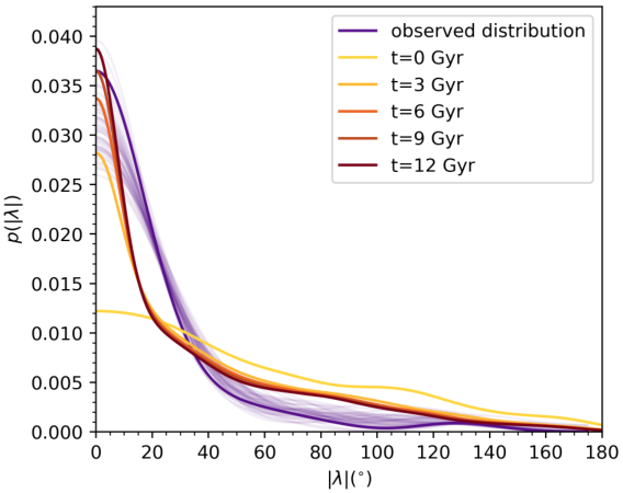
We fit a kernel density estimation (KDE) to the distributions of host star , age, , and for the 33 planets in our sample that orbit stars below the Kraft break, then drew random values from each of these smoothed distributions to produce a set of 10,000 simulated systems. All systems were initialized with . We assumed a linear damping rate, and we set in in accordance with Figure 3.
We ultimately found that the distribution evolves along the pathway shown in Figure 4 as a result of tidal damping. The theoretical KDE at Gyr shows a peak at low obliquities analogous to that of the observed distribution. Minor discrepancies at moderate values may result from the small number of misaligned planets (five planets with ) that shape the tail of the smoothed, observed sample, without necessarily indicating a true disagreement between the two distributions.
The sky-projected obliquities were directly evolved under the implicit assumption that . At low values, acts as a lower limit on , whereas is more likely to be close to for larger values (Fabrycky & Winn 2009). This bias indicates that some fraction of systems observed with low sky-projected obliquities should actually have larger 3D obliquities. Because the probability density peaks at even for low measured values (see Figure 3 of Fabrycky & Winn 2009), the distribution should not change dramatically if the true distribution was evolved rather than the sky-projected distribution .
Our proof-of-concept shows that tidal damping can reproduce the current distribution of observed cool star obliquities based on an initial model comprised of secular mechanisms, without the requirement of invoking disk migration or in-situ formation. We emphasize that we do not rule out contributions from these mechanisms, but, rather, we show that they are not stricly required to account for the stellar obliquity distribution. Minor adjustments to the weighting of secular processes can reproduce the circular hot star distribution and the two eccentric distributions in Figure 2, each of which has been relatively unaffected by damping.
IV The Role of Orbital Eccentricity
The eccentricities of misaligned systems provide an independent test of high-eccentricity migration. While our analysis up to this point has focused on the stellar obliquity damping timescale , we can also consider the timescale, , for eccentricity evolution driven by tidal dissipation within the planet. Under the effects of tidal dissipation, the evolution of a planet’s eccentricity is given by
| (6) |
where is the host star mass, is the mass of the planet, and is the orbital energy of the planet.
The rate of energy dissipation for a synchronously rotating planet is
| (7) |
Here, is the planet’s effective tidal dissipation parameter, is the planet’s Love number, and is the pseudosynchronous rotation rate, given by
| (8) |
where is the mean motion of the planet’s orbit. We set and . The corrective factor , derived in Wisdom 2008, is defined as
| (9) |
where
| (10) |
| (11) |
| (12) |
| (13) |
Separating the 60 planets in Figure 3 into four evenly sized bins of 15 planets each, ordered by , we demonstrate that systems with shorter also preferentially have shorter such that their eccentricities and obliquities should be jointly damped over the lifetime of the system. is typically shorter than such that hot Jupiters should often circularize before realigning. In contrast, systems with the longest , which include most of the population, have values exceeding the age of the system. Both timescales, which are contributed by two independent processes – damping within the planet and damping within the star – are therefore consistent with the observed distributions. If all systems formed through high-eccentricity migration, the observed and distributions would look as they do today.
V Implications for Hot Jupiter Formation Theory
Our results provide two key constraints on the obliquity distribution of Rossiter-McLaughlin targets, which are primarily hot Jupiter host stars. The first constraint, which is a variation on previous findings (Winn et al. 2010; Schlaufman 2010), is the observation that stars hosting circular hot Jupiters span a wider range of obliquities above the Kraft break than at lower temperatures. The second is the absence of this pattern in the eccentric sample, where obliquities are consistent with no change at the Kraft break. Together, these observations demonstrate that the population of hot Jupiters is consistent with formation through high-eccentricity migration and suggest that dissipative mechanisms are vital for shaping the obliquity distribution of hot Jupiter host stars.
The absence of a significant change in obliquities at the Kraft break for eccentric systems indicates that dissipative mechanisms have not had time to sculpt the eccentric population in the same way that they have shaped the circular population. In the framework of Kozai capture (Naoz et al. 2012), eccentric planets are either experiencing ongoing eccentric Kozai-Lidov oscillations or they have had these oscillations suppressed by apsidal precession in the past. Our sample includes well-characterized systems such as that of HD 80606, in which the transiting planet’s high obliquity and eccentricity are cleanly recovered through Kozai migration (Wu & Murray 2003).
A subset of eccentric planets that have two or more planetary companions may be undergoing secular chaos. Secular chaos transfers angular momentum outwards due to the overlap of resonances in a multiplanet system, elevating the orbital inclination and eccentricity of the innermost planet. In either excitation framework, tidal dissipation, which acts differentially in hot and cool star systems, has not had time to globally alter the distribution of the eccentric population.
For hot Jupiter systems with circular orbits, tidal dissipation has played a more important role in shaping the currently observed stellar obliquity distribution. These systems are consistent with -body interactions that were suppressed early on such that the companion orbits were able to fully tidally circularize and, in some cases, realign. Planets orbiting cool stars realign quickly, while those orbiting hot stars have much longer tidal realignment timescales and remain closer to their primordial spin-orbit angles.
Systems with both large misalignments and high eccentricities may instead be produced by a combination of primordial disk misalignments and planet-planet or planet-disk interactions (Duffell & Chiang 2015; Anderson & Lai 2017; Frelikh et al. 2019; Anderson et al. 2020; Debras et al. 2021). Our results do not rule out these alternative scenarios, but, rather, they provide a relatively simple framework that is fully consistent with the observed and distributions. Previous work has revealed that long-period ( day) planets orbiting hot stars tentatively demonstrate a trend towards alignment (Rice et al. 2021). Because these planets are exceptionally difficult to realign through tidal interactions, this trend, if confirmed, may suggest that protoplanetary disks are typically aligned and that the misalignments of hot Jupiters are attained through dynamical interactions after the disk has dispersed.
VI Conclusions
Our analysis establishes that the observed distribution of hot Jupiter host star obliquities can arise naturally from a combination of high-eccentricity migration and obliquity damping mechanisms. Cool stars hosting circular planets have had the most strongly damped obliquities, while hot stars and hosts of eccentric planets have experienced weaker damping. We predict that, under our proposed framework, the observed difference between the eccentric and cumulative sums will grow with additional observations. We conclude that the stellar obliquity distribution for hot Jupiter systems is consistent with having been crafted primarily by high-eccentricity migration and tidal damping, with no requirement to appeal to disk migration or in-situ formation at the population level.
VII Acknowledgements
M.R. is supported by the National Science Foundation Graduate Research Fellowship Program under Grant Number DGE-1752134. This research has made use of the NASA Exoplanet Archive, which is operated by the California Institute of Technology, under contract with the National Aeronautics and Space Administration under the Exoplanet Exploration Program.
Exoplanet Archive, Extrasolar Planets Encyclopaedia, Open Exoplanet Catalogue
Appendix A Adopted Parameters
Our full samples of parameters, drawn from archival studies, are provided as supplementary data for Figure 1. All stellar and planetary parameters other than stellar multiplicity and were drawn directly from the NASA Exoplanet Archive, with ages supplemented by the Extrasolar Planets Encylopaedia. The stellar multiplicity of each system, provided for reference, was determined through cross-matching with the Catalogue of Exoplanets in Binary Star Systems (Schwarz et al. 2016) and the Open Exoplanet Catalogue.
Appendix B Orbital Period vs. Eccentricity
One alternative possibility is that eccentricity acts as a proxy for a different trend in the dataset. The tidal circularization timescale of a short-period planet scales with semimajor axis as (Murray & Dermott 1999), meaning that small differences in semimajor axis correspond to dramatically different tidal circularization timescales. Planets on eccentric orbits, by definition, have not completed the tidal circularization process. This means that they may also tend to have larger semimajor axes, or, equivalently, longer orbital periods () as compared with planets.
To address this possibility, we carried out the same analysis as a function of orbital period (comparing the day and day populations) and as a function of orbital separation (comparing the and populations), with results shown in Figure 5. If the observed effect is predominantly due to a correlation between obliquity and orbital period (orbital separation), rather than eccentricity, the population should show a stronger increase in misalignments with increasing () than .

In both cases, the significance of our result was substantially weaker than when dividing the sample by eccentricity (), with only a signal when segmenting by and a signal when segmenting by . Figure 5 also shows substantial structure below the Kraft break in the day and sums. This suggests that divisions by or may produce a more heterogeneous population than that produced by our eccentricity cut, where planets smoothly follow a relatively consistent upward trend in .
Finally, both panels of Figure 5 reveal a nearly flat trend in above the Kraft break. This demonstrates that relatively long-period systems around hot stars have typically been observed to be aligned, as pointed out in Rice et al. 2021.
References
- Akaike (1973) Akaike, H. 1973, Biometrika, 60, 255
- Albrecht et al. (2012) Albrecht, S., Winn, J. N., Johnson, J. A., et al. 2012, The Astrophysical Journal, 757, 18
- Anderson & Lai (2017) Anderson, K. R., & Lai, D. 2017, Monthly Notices of the Royal Astronomical Society, 472, 3692
- Anderson et al. (2020) Anderson, K. R., Lai, D., & Pu, B. 2020, Monthly Notices of the Royal Astronomical Society, 491, 1369
- Anderson et al. (2016) Anderson, K. R., Storch, N. I., & Lai, D. 2016, Monthly Notices of the Royal Astronomical Society, 456, 3671
- Batygin et al. (2016) Batygin, K., Bodenheimer, P. H., & Laughlin, G. P. 2016, The Astrophysical Journal, 829, 114
- Beaugé & Nesvornỳ (2012) Beaugé, C., & Nesvornỳ, D. 2012, The Astrophysical Journal, 751, 119
- Boley et al. (2016) Boley, A. C., Contreras, A. G., & Gladman, B. 2016, The Astrophysical Journal Letters, 817, L17
- Bryan et al. (2016) Bryan, M. L., Knutson, H. A., Howard, A. W., et al. 2016, The Astrophysical Journal, 821, 89
- Dawson (2014) Dawson, R. I. 2014, The Astrophysical Journal Letters, 790, L31
- Dawson & Johnson (2018) Dawson, R. I., & Johnson, J. A. 2018, Annual Review of Astronomy and Astrophysics, 56, 175
- Debras et al. (2021) Debras, F., Baruteau, C., & Donati, J.-F. 2021, Monthly Notices of the Royal Astronomical Society, 500, 1621
- Duffell & Chiang (2015) Duffell, P. C., & Chiang, E. 2015, The Astrophysical Journal, 812, 94
- Fabrycky & Tremaine (2007) Fabrycky, D., & Tremaine, S. 2007, The Astrophysical Journal, 669, 1298
- Fabrycky & Winn (2009) Fabrycky, D. C., & Winn, J. N. 2009, The Astrophysical Journal, 696, 1230
- Foreman-Mackey et al. (2013) Foreman-Mackey, D., Hogg, D. W., Lang, D., & Goodman, J. 2013, PASP, 125, 306
- Frelikh et al. (2019) Frelikh, R., Jang, H., Murray-Clay, R. A., & Petrovich, C. 2019, The Astrophysical Journal Letters, 884, L47
- Goldreich & Tremaine (1980) Goldreich, P., & Tremaine, S. 1980, Astrophysical Journal, 241, 425
- Hamers et al. (2017) Hamers, A. S., Antonini, F., Lithwick, Y., Perets, H. B., & Portegies Zwart, S. F. 2017, Monthly Notices of the Royal Astronomical Society, 464, 688
- Harris et al. (2020) Harris, C. R., Millman, K. J., van der Walt, S. J., et al. 2020, Nature, 585, 357
- Hunter (2007) Hunter, J. D. 2007, Computing in science & engineering, 9, 90
- Hurvich & Tsai (1989) Hurvich, C. M., & Tsai, C.-L. 1989, Biometrika, 76, 297
- Kraft (1967) Kraft, R. P. 1967, The Astrophysical Journal, 150, 551
- Lin et al. (1996) Lin, D. N., Bodenheimer, P., & Richardson, D. C. 1996, Nature, 380, 606
- Lin & Papaloizou (1986) Lin, D. N., & Papaloizou, J. 1986, The Astrophysical Journal, 309, 846
- Lin & Ogilvie (2017) Lin, Y., & Ogilvie, G. I. 2017, Monthly Notices of the Royal Astronomical Society, 468, 1387
- Lucy & Sweeney (1971) Lucy, L., & Sweeney, M. 1971, The Astronomical Journal, 76, 544
- McKinney et al. (2010) McKinney, W., et al. 2010, in Proceedings of the 9th Python in Science Conference, Vol. 445, Austin, TX, 51–56
- McLaughlin (1924) McLaughlin, D. 1924, The Astrophysical Journal, 60
- Millholland et al. (2017) Millholland, S., Wang, S., & Laughlin, G. 2017, The Astrophysical Journal Letters, 849, L33
- Murray & Dermott (1999) Murray, C. D., & Dermott, S. F. 1999, Solar system dynamics (Cambridge university press)
- Nagasawa & Ida (2011) Nagasawa, M., & Ida, S. 2011, The Astrophysical Journal, 742, 72
- Nagasawa et al. (2008) Nagasawa, M., Ida, S., & Bessho, T. 2008, The Astrophysical Journal, 678, 498
- Naoz et al. (2011) Naoz, S., Farr, W. M., Lithwick, Y., Rasio, F. A., & Teyssandier, J. 2011, Nature, 473, 187
- Naoz et al. (2012) Naoz, S., Farr, W. M., & Rasio, F. A. 2012, The Astrophysical Journal Letters, 754, L36
- Ngo et al. (2015) Ngo, H., Knutson, H. A., Hinkley, S., et al. 2015, ApJ, 800, 138
- Ogilvie (2014) Ogilvie, G. I. 2014, Annual Review of Astronomy and Astrophysics, 52, 171
- Oliphant (2006) Oliphant, T. E. 2006, A guide to NumPy, Vol. 1 (Trelgol Publishing USA)
- Petrovich (2015) Petrovich, C. 2015, The Astrophysical Journal, 799, 27
- Petrovich & Tremaine (2016) Petrovich, C., & Tremaine, S. 2016, The Astrophysical Journal, 829, 132
- Pinsonneault et al. (2001) Pinsonneault, M., DePoy, D., & Coffee, M. 2001, The Astrophysical Journal Letters, 556, L59
- Rasio & Ford (1996) Rasio, F. A., & Ford, E. B. 1996, Science, 274, 954
- Rice et al. (2021) Rice, M., Wang, S., Howard, A. W., et al. 2021, The Astronomical Journal, 162, 182
- Rogers et al. (2012) Rogers, T., Lin, D. N., & Lau, H. H. B. 2012, The Astrophysical Journal Letters, 758, L6
- Rossiter (1924) Rossiter, R. 1924, The Astrophysical Journal, 60
- Schlaufman (2010) Schlaufman, K. C. 2010, The Astrophysical Journal, 719, 602
- Schwarz et al. (1978) Schwarz, G., et al. 1978, Annals of statistics, 6, 461
- Schwarz et al. (2016) Schwarz, R., Funk, B., Zechner, R., & Bazsó, Á. 2016, Monthly Notices of the Royal Astronomical Society, 460, 3598
- Southworth (2011) Southworth, J. 2011, Monthly Notices of the Royal Astronomical Society, 417, 2166
- Spalding & Batygin (2015) Spalding, C., & Batygin, K. 2015, The Astrophysical Journal, 811, 82
- Teyssandier et al. (2019) Teyssandier, J., Lai, D., & Vick, M. 2019, Monthly Notices of the Royal Astronomical Society, 486, 2265
- Vick et al. (2019) Vick, M., Lai, D., & Anderson, K. R. 2019, Monthly Notices of the Royal Astronomical Society, 484, 5645
- Virtanen et al. (2020) Virtanen, P., Gommers, R., Oliphant, T. E., et al. 2020, Nature methods, 17, 261
- Walt et al. (2011) Walt, S. v. d., Colbert, S. C., & Varoquaux, G. 2011, Computing in Science & Engineering, 13, 22
- Wang et al. (2021a) Wang, S., Winn, J. N., Addison, B. C., et al. 2021a, arXiv preprint arXiv:2105.12902
- Wang et al. (2021b) Wang, X.-Y., Rice, M., Wang, S., et al. 2021b, arXiv preprint arXiv:2110.08832
- Weiss et al. (2018) Weiss, L. M., Marcy, G. W., Petigura, E. A., et al. 2018, The Astronomical Journal, 155, 48
- Winn et al. (2010) Winn, J. N., Fabrycky, D., Albrecht, S., & Johnson, J. A. 2010, The Astrophysical Journal Letters, 718, L145
- Wisdom (2008) Wisdom, J. 2008, Icarus, 193, 637
- Wu & Lithwick (2011) Wu, Y., & Lithwick, Y. 2011, The Astrophysical Journal, 735, 109
- Wu & Murray (2003) Wu, Y., & Murray, N. 2003, The Astrophysical Journal, 589, 605
- Wu et al. (2007) Wu, Y., Murray, N. W., & Ramsahai, J. M. 2007, The Astrophysical Journal, 670, 820
- Zakamska et al. (2011) Zakamska, N. L., Pan, M., & Ford, E. B. 2011, Monthly Notices of the Royal Astronomical Society, 410, 1895