Polynomials with many rational preperiodic points

John R. Doyle Address: Dept. of Mathematics
Oklahoma State University
Stillwater, OK 74078 Email address: john.r.doyle@okstate.edu and Trevor Hyde Address: Dept. of Mathematics
University of Chicago
Chicago, IL 60637 Email address: tghyde@uchicago.edu

Abstract.

In this paper we study two questions related to exceptional behavior of preperiodic points of polynomials in $\mathbb{Q}[x]$ . We show that for all $d\geq 2$ , there exists a polynomial $f_{d}(x)\in\mathbb{Q}[x]$ with $2\leq\deg(f_{d})\leq d$ such that $f_{d}(x)$ has at least $d+\lfloor\log_{2}(d)\rfloor$ rational preperiodic points. Furthermore, we show that for infinitely many integers $d$ , the polynomials $f_{d}(x)$ and $f_{d}(x)+1$ have at least $d^{2}+d\lfloor\log_{2}(d)\rfloor-2d+1$ common complex preperiodic points.

1. Introduction

Let $K$ be a field and let $f(x)\in K[x]$ be a polynomial. We write $f^{n}(x)$ to denote the $n$ -fold composition of $f$ with itself. A point $\alpha\in\overline{K}$ is preperiodic under $f(x)$ if the orbit $\{f^{n}(\alpha):n\geq 0\}$ is finite. Let $\mathrm{PrePer}(f,K)$ denote the set of $K$ -rational preperiodic points of $f$ ,

\mathrm{PrePer}(f,K):=\{\alpha\in K:\alpha\text{ is preperiodic under }f\}.

The following questions arise naturally in arithmetic and complex dynamics:

Question 1.1.

How many rational preperiodic points can a degree- $d$ polynomial $f(x)\in\mathbb{Q}[x]$ have?

Question 1.2.

How many complex preperiodic points can degree- $d$ polynomials $f(x),g(x)\in\mathbb{C}[x]$ have in common?

Both questions are conjectured to have answers in the form of uniform upper bounds depending only on $d$ (subject to some minor caveats described below). Our main result proves the existence of a sequence of polynomials $f_{d}(x)\in\mathbb{Q}[x]$ of degree at most $d$ which simultaneously exhibit extremal behavior for both questions: $f_{d}(x)$ has many rational preperiodic points, and the polynomials $f_{d}(x)+i$ and $f_{d}(x)+j$ have many common complex preperiodic points for small integers $i$ and $j$ .

Theorem 1.3.

For all integers $d\geq 2$ there exists a polynomial $f_{d}(x)\in\mathbb{Q}[x]$ such that $2\leq\deg(f)\leq d$ and

(1)

$f_{d}(x)$ has at least $d+\lfloor\log_{2}(d)\rfloor$ rational preperiodic points,
(2)

for all $0\leq i<j\leq\log_{2}(d)$ ,

$\Big|\mathrm{PrePer}(f_{d}(x)+i,\mathbb{C})\cap\mathrm{PrePer}(f_{d}(x)+j,\mathbb{C})\Big|<\infty,$
(3)

and

$\left|\bigcap_{i=0}^{\lfloor\log_{2}(d)\rfloor}\mathrm{PrePer}(f_{d}(x)+i,\mathbb{C})\right|\geq\deg(f_{d})(d-1)+1.$

Remark.

Using Lagrange interpolation one may easily construct degree- $d$ polynomials with $d+1$ rational preperiodic points. Each rational preperiodic point beyond $d+1$ imposes an additional constraint. Theorem 1.3 shows that it is possible to get an improvement on the order of (at least) $\log(d)$ on the Lagrange interpolation construction.

Given an integer $d\geq 2$ , let

	$\displaystyle B_{d}$	$\displaystyle:=\sup_{f}\|\mathrm{PrePer}(f,\mathbb{Q})\|\in[0,\infty],$
	$\displaystyle C_{d}$	$\displaystyle:=\sup_{f,g}\|\mathrm{PrePer}(f,\mathbb{C})\cap\mathrm{PrePer}(g,\mathbb{C})\|\in[0,\infty],$

where the supremum defining $B_{d}$ is taken over all polynomials $f(x)\in\mathbb{Q}[x]$ with $2\leq\deg(f)\leq d$ , and the supremum defining $C_{d}$ is taken over all $f(x),g(x)\in\mathbb{C}[x]$ with $2\leq\deg(f),\deg(g)\leq d$ such that $\mathrm{PrePer}(f,\mathbb{C})\neq\mathrm{PrePer}(g,\mathbb{C})$ . Both $B_{d}$ and $C_{d}$ are conjectured to be finite for all $d\geq 2$ .

Northcott [18] proved that if $\deg(f)\geq 2$ , then $\mathrm{PrePer}(f,\mathbb{Q})$ is finite. The Morton-Silverman Uniform Boundedness Conjecture [17, p. 100] asserts, in part, that $B_{d}<\infty$ . This conjecture has motivated a substantial volume of work in arithmetic dynamics (see Silverman [20, Sec. 3.3]). While it is widely believed to be true, the Uniform Boundedness Conjecture has yet to be proved unconditionally in any degree. Looper [14] recently gave a conditional proof that $B_{d}<\infty$ , assuming a generalization of the $abc$ conjecture.

DeMarco, Krieger, and Ye [8, Conj. 1.4] conjecture that $C_{d}<\infty$ for all $d\geq 2$ ; they prove this conjecture when $f$ and $g$ are restricted to the family of quadratic polynomials of the form $x^{2}+c$ [8, Thm. 1.1]. Mavraki and Schmidt [15] recently proved an analogous uniform bound on the number of common preperiodic points along 1-parameter families in $\mathrm{Rat}_{d}\times\mathrm{Rat}_{d}$ , where $\mathrm{Rat}_{d}$ denotes the space of degree- $d$ rational functions.

The polynomials asserted to exist in Theorem 1.3 combined with an explicit family described below in Theorem 1.10 lead to the following lower bounds on $B_{d}$ and $C_{d}$ .

Corollary 1.4.

For all integers $d\geq 2$ ,

(1)

$B_{d}\geq d+\max(6,\lfloor\log_{2}(d)\rfloor)$ ,
(2)

$C_{d}\geq d^{2}+4d+1$ .

Furthermore, there are infinitely many $d\geq 2$ for which

C_{d}\geq d^{2}+d\lfloor\log_{2}(d/4)\rfloor+1.

One may compare Corollary 1.4(1) to known lower bounds on $A_{g}:=\sup_{X}|X(\mathbb{Q})|$ , where $X$ ranges over all smooth irreducible genus- $g$ curves defined over $\mathbb{Q}$ . In this setting, the best known lower bound for $A_{g}$ that holds for all $g\geq 2$ is linear in $g$ (see [5]), though it is unknown whether the correct upper bound should also be linear. In that spirit, we pose the following question:

Question 1.5.

What is the order of growth of $B_{d}$ as $d\to\infty$ ? Is it true that

B_{d}=d+O(\log(d))?

Remark.

Our proof of Theorem 1.3(3) (hence also Corollary 1.4(2)) actually shows something stronger: Given a set $\mathcal{P}$ of polynomials, we say that a finite set $S\subseteq\mathbb{C}$ has a finite orbit under $\mathcal{P}$ if $f(S)\subseteq S$ for every $f\in\mathcal{P}$ . (See [3] for a detailed study of finite orbits for pairs of quadratic and cubic polynomials.) Note that if $S$ has a finite orbit under $\mathcal{P}$ , then $S\subseteq\bigcap_{f\in\mathcal{P}}\mathrm{PrePer}(f,\mathbb{C})$ , but, in general, common preperiodic points of the elements of $\mathcal{P}$ need not have a finite orbit under $\mathcal{P}$ .

With this setup, we prove that for the polynomials $f_{d}(x)\in\mathbb{Q}[x]$ provided by Theorem 1.3, the set of maps $\mathcal{P}:=\{f_{d}(x)+i:0\leq i\leq\lfloor\log_{2}(d)\rfloor\}$ has a finite orbit with at least $\deg(f_{d})(d-1)+1$ elements. As a result, it follows that Corollary 1.4(2) holds when $C_{d}$ is replaced with

\widetilde{C}_{d}:=\sup_{f,g}\sup_{S}|S|\leq C_{d},

where $f$ and $g$ range over all polynomials of degree $2\leq\deg(f),\ \deg(g)\leq d$ such that $\mathrm{PrePer}(f,\mathbb{C})\neq\mathrm{PrePer}(g,\mathbb{C})$ and $S$ ranges over all finite orbits of $\mathcal{P}=\{f,g\}$ .

Remark.

The two uniform boundedness conjectures stated above for polynomials are believed to hold more generally for rational functions on $\mathbb{P}^{1}$ . However, the methods of this paper appear to be constrained to polynomials. Note that if $B_{d}^{\prime}$ and $C_{d}^{\prime}$ are defined analogously to $B_{d}$ and $C_{d}$ , but with rational functions instead of polynomials, then we have $B_{d}<B_{d}^{\prime}$ and $C_{d}<C_{d}^{\prime}$ for all $d\geq 2$ . This inequality follows from the simple observation that every polynomial is a rational function, plus the fact that we are not counting $\infty$ as a preperiodic point, though it is a fixed point for every polynomial map when considered as an endomorphism of $\mathbb{P}^{1}$ .

Remark.

Fu and Stoll [10] recently proved a result analogous to Corollary 1.4(2), giving lower bounds on the maximal number of common torsion $x$ -coordinates for pairs of elliptic curves $E_{1},E_{2}$ such that $x(E_{1,\mathrm{tors}})\neq x(E_{2,\mathrm{tors}})$ . Their results have the following dynamical interpretation: If $f_{i}(x)$ denotes the degree-4 flexible Lattès map associated to multiplication by $2$ on the elliptic curve $E_{i}$ , then $x(E_{i,\mathrm{tors}})=\mathrm{PrePer}(f_{i}(x),\mathbb{C})$ . Hence [10, Thm. 2] implies that there are infinitely many pairs of elliptic curves $E_{1}$ , $E_{2}$ for which

22\leq|\mathrm{PrePer}(f_{1}(x),\mathbb{C})\cap\mathrm{PrePer}(f_{2}(x),\mathbb{C}))|<\infty,

and [10, Thm. 3] implies that there exists an explicit pair of elliptic curves $E_{1}$ , $E_{2}$ such that

(1.1)

|\mathrm{PrePer}(f_{1}(x),\mathbb{C})\cap\mathrm{PrePer}(f_{2}(x),\mathbb{C}))|=34.

Using the notation of the previous remark, (1.1) implies that $C_{4}^{\prime}\geq 34$ . On the other hand, in Section 5 we provide an example that shows that $C_{4}\geq 36$ , hence that $C_{4}^{\prime}\geq 37$ .

Remark.

Despite the considerable interest in proving $B_{d}<\infty$ , we are unaware of any previous work explicitly proving nontrivial lower bounds on $B_{d}$ outside of finitely many low degree cases. However, motivated by problems in complexity theory, Cohen, Shpilka, and Tal prove a result ([7, Thm. 1.5]; see also [7, p. 458]) that implies the following: For all $0<\varepsilon<1$ , there exists $d_{\varepsilon}$ such that for all $d\geq d_{\varepsilon}$ , we have

B_{d}\geq d+\lfloor\varepsilon\log_{2}(d)\rfloor.

Our improvement on this lower bound in Corollary 1.4(1) stems from an exact evaluation of a certain lattice discriminant (see Theorem 2.1) that was only bounded in [7]. We thank Yan Sheng Ang for bringing [7] to our attention.

1.1. Dynamical compression

For a positive integer $m$ , let $[m]:=\{1,2,3,\ldots,m\}$ . We say a degree- $d$ polynomial $g(x)\in\mathbb{C}[x]$ exhibits dynamical compression if $g(x)$ is conjugate to some polynomial $f(x)$ —that is, $f=\ell\circ g\circ\ell^{-1}$ for some linear polynomial $\ell(x)\in\mathbb{C}[x]$ —which satisfies

f([m])\subseteq[n]

for some $m\geq n>d+1$ . In this case, $[m]\subseteq\mathrm{PrePer}(f(x),\mathbb{Q})$ . The polynomials $f_{d}(x)$ asserted to exist in Theorem 1.3 all exhibit dynamical compression.

Example 1.6.

Let $f(x):=\frac{x^{2}-9x+22}{2}$ . One may check that

(1.2)

f([8])\subseteq[7].

Therefore, both $f(x)$ and $f(x)+1$ exhibit dynamical compression and have at least 8 rational preperiodic points, namely the elements of $[8]$ . In fact, it may be shown that $f(x)$ and $f(x)+1$ have exactly 8 rational preperiodic points. Hence $B_{2}\geq 8$ ; in fact, Poonen [19] has conjectured that $B_{2}=8$ . The polynomials $f(x)$ and $f(x)+1$ are simultaneously conjugate to $x^{2}-\frac{29}{16}$ and $x^{2}-\frac{21}{16}$ , respectively. These quadratic polynomials appear several times in the literature for their exceptional properties, including in DeMarco, Krieger, and Ye [8], Doyle, Faber and Krumm [9], Hindes [13], Morton and Raianu [16], and Poonen [19].

Example 1.7.

The cubic polynomial $f(x):=\frac{x^{3}-18x^{2}+89x-66}{6}$ satisfies $f([11])\subseteq[11]$ . Thus both $f(x)$ and $12-f(x)$ exhibit dynamical compression and have at least 11 rational preperiodic points. These examples share the current record with 8 other cubics, found by computational search in Benedetto et al. [2, Table 2], for the cubic polynomial with the most rational preperiodic points. Of the 10 record-holding cubics found by Benedetto et al., only the two conjugate to $f(x)$ and $12-f(x)$ exhibit dynamical compression.

The following proposition, proved in Section 3, makes explicit the connection between dynamical compression and polynomials with many common preperiodic points.

Proposition 1.8.

Suppose that $f(x)\in\mathbb{C}[x]$ is a degree $d\geq 2$ polynomial such that

f([m])\subseteq[n],

for some integers $m>n\geq 1$ . Then

d(n-1)+1\leq\Big|\bigcap_{i=0}^{m-n}\mathrm{PrePer}(f(x)+i,\mathbb{C})\Big|<\infty.

Example 1.9.

Returning to Example 1.6, let $f(x):=\frac{x^{2}-9x+22}{2}$ . Then (1.2) and Proposition 1.8 imply that

|\mathrm{PrePer}(f(x),\mathbb{C})\cap\mathrm{PrePer}(f(x)+1,\mathbb{C})|\geq 13.

However, by comparing the preperiodic points with small forward orbit for $f(x)$ and $f(x)+1$ directly, we find that $\mathrm{PrePer}(f(x),\mathbb{C})\cap\mathrm{PrePer}(f(x)+1,\mathbb{C})$ actually contains at least 26 points. Hence $C_{2}\geq 26$ . That is, dynamical compression accounts for half of the known preperiodic points shared by $f(x)$ and $f(x)+1$ . To the best of our knowledge, this is the current record for a lower bound on $C_{2}$ . See Table 3 in Section 5 for more lower bound records on $C_{d}$ for $2\leq d\leq 15$ .

The proof of Theorem 1.3 uses a geometry of numbers approach to show the existence of polynomials which compress exceptionally large intervals of integers but does not produce explicit examples. Thus it remains an interesting problem to construct explicit polynomials which surpass the trivial lower bounds on $B_{d}$ and $C_{d}$ . Our last result provides one such family $r_{d}(x)$ . Formulas for $r_{d}(x)$ are given in Section 4.

Theorem 1.10.

For all $d\geq 2$ , there is an explicit degree- $d$ polynomial $r_{d}(x)$ such that

r_{d}([d+6])\subseteq\begin{cases}[d+5]&\text{if $d$ is even,}\\ [d+4]&\text{if $d$ is odd.}\end{cases}

1.2. Acknowledgements

We thank Laura DeMarco for a helpful correspondence which prompted this work. We thank Hang Fu for pointing out that (1.1) follows from [10, Thm. 3]. We thank Joseph Silverman for several helpful comments on an earlier draft, as well as for suggesting that we include the discussion and question immediately following Corollary 1.4. We thank Yan Sheng Ang for bringing the article [7] to our attention. And we thank the University of Chicago Research Computing Center for access to their high performance computing cluster. John Doyle was partially supported by NSF grant DMS-2112697. Trevor Hyde was partially supported by the NSF Postdoctoral Research Fellowship DMS-2002176 and the Jump Trading Mathlab Research Fund.

2. Rational Preperiodic Points

The goal of this section is to prove Theorem 1.3, which is stated in a refined form below as Theorem 2.5. Our strategy is to consider the lattice $\Lambda_{d,e}$ generated by vectors of the form $(f(0),f(1),\ldots,f(d+e))$ where $f(x)$ is a degree-at-most- $d$ integer-valued polynomial and $e>0$ is an integer. (Fecall that $g(x)\in\mathbb{Q}[x]$ is said to be integer-valued if $g(\mathbb{Z})\subseteq\mathbb{Z}$ .) There is a natural bijection between vectors in $\Lambda_{d,e}$ contained within a small box near the origin and degree-at-most- $d$ polynomials exhibiting dynamical compression. We use a classical geometry-of-numbers theorem of Minkowski to prove the existence of lattice points in this box by analyzing the discriminant of $\Lambda_{d,e}$ .

2.1. Lattices and their discriminants

Let $m\geq 1$ be an integer. By a lattice $\Lambda\subseteq\mathbb{R}^{m}$ we mean a discrete free abelian subgroup of $\mathbb{R}^{m}$ . If $\Lambda$ is a rank $n$ lattice with basis $v_{1},v_{2},\ldots,v_{n}$ , then we call the compact set $\{\sum_{i=1}^{n}c_{i}v_{i}:0\leq c_{i}\leq 1\}$ a fundamental domain of $\Lambda$ . The discriminant of $\Lambda$ , which we denote by $\delta(\Lambda)$ is the square of the $n$ -dimensional volume of a fundamental domain of $\Lambda$ . If $M$ is the matrix with rows $v_{i}$ , then

\delta(\Lambda)=\det(MM^{T}).

Note that $\delta(\Lambda)$ is independent of the choice of basis for $\Lambda$ .

Given integers $d,e\geq 0$ , let $\Lambda_{d,e}$ be the lattice in $\mathbb{R}^{d+e+1}$ spanned by the $d+1$ vectors

u_{i}:=\left(\binom{0}{i},\binom{1}{i},\ldots,\binom{d+e}{i}\right)\in\mathbb{Z}^{d+e+1}

for $0\leq i\leq d$ . (Note that $\binom{j}{i}=0$ if $j<i$ .) The lattice $\Lambda_{d,e}$ has rank $d+1$ : Indeed, if $\sum_{i=0}^{d}a_{i}u_{i}=0$ , then the degree-at-most- $d$ polynomial $\sum_{i=0}^{d}a_{i}\binom{x}{i}$ vanishes at more than $d$ points (namely, the points $0,1,2,\ldots,d+e$ ), hence all of the coefficients must be zero. We now provide an explicit formula for $\delta(\Lambda_{d,e})$ .

Theorem 2.1.

The discriminant of $\Lambda_{d,e}$ is given by

\delta(\Lambda_{d,e})=\prod_{i=0}^{d}\prod_{j=1}^{e}\frac{d+i+j+1}{i+j}.

Proof.

Let $M_{d,e}=\big(\binom{j}{i}\big)$ be the $(d+1)\times(d+e+1)$ matrix with rows $u_{i}$ . Thus,

\delta(\Lambda_{d,e})=\det(M_{d,e}M_{d,e}^{T}).

To evaluate $\delta(\Lambda_{d,e})$ we use the Lindström-Gessel-Viennot lemma [12, Thm. 1] to interpret $\det(M_{d,e}M_{d,e}^{T})$ as the number of plane partitions which fit inside a $(d+1)\times(d+1)\times e$ box. The number of such plane partitions is given by MacMahon’s formula, which provides the desired product formula for $\delta(\Lambda_{d,e})$ .

A plane partition $\Pi$ is a finite, weakly increasing sequence of partitions $\lambda_{1}\leq\lambda_{2}\leq\cdots\leq\lambda_{k}$ . More intuitively, a plane partition may be thought of us a finite set of boxes stacked in the corner of a room. For example, the plane partition in Figure 1 may be visualized as the stack of boxes in Figure 2.

Given positive integers $r,s,t$ , we say a plane partition $\Pi:\lambda_{1}\leq\lambda_{2}\leq\cdots\leq\lambda_{k}$ fits inside the $r\times s\times t$ box if $k\leq t$ and if the Young diagram of $\lambda_{k}$ fits inside an $r\times s$ box. Equivalently, the box diagram of $\Pi$ fits inside an $r\times s\times t$ box. Let $N(r,s,t)$ denote the number of plane partitions which fit inside an $r\times s\times t$ box. We claim that $\delta(\Lambda_{d,e})=N(d+1,d+1,e)$ .

Let $\mathcal{I}$ be the $\mathbb{Z}$ -lattice in $\mathbb{R}^{2}$ spanned by the vectors $v_{1}:=(-\sqrt{3},1)$ and $v_{2}:=(\sqrt{3},1)$ . Let $v_{3}:=v_{1}+v_{2}=(0,2)\in\mathcal{I}$ . Given positive integers $a,b,c$ , let $H(a,b,c)$ denote the convex hull of the six points

\{0,av_{1},bv_{2},av_{1}+cv_{3},bv_{2}+cv_{3},av_{1}+bv_{2}+cv_{3}\}\subseteq\mathcal{I}.

See Figure 3 for an illustration. There is a simple and well-known correspondence between plane partitions that fit inside a box of dimensions $a\times b\times c$ and rhombic tilings of $H(a,b,c)$ (see Figure 4). This correspondence comes from the interpretation of a plane partition as a stack of cubical blocks in a the first quadrant of $\mathbb{R}^{3}$ and viewing this stack of blocks from along the ray spanned by $(1,1,1)$ .

Refer to caption — Figure 1. Example of a plane partition, illustrated using Young diagrams.

Now consider a plane partition $\Pi$ contained in a box of size $(d+1)\times(d+1)\times e$ viewed as a rhombic tiling of $H(d+1,d+1,e)$ . There are three types of rhombic tiles $T_{i}$ , characterized by which $v_{i}$ is parallel to the short diagonal of $T_{i}$ ; see Figure 7.

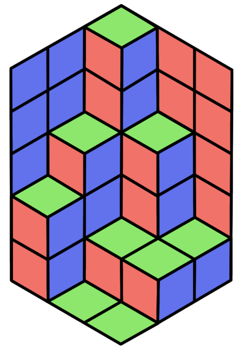
For each $0\leq i\leq d$ , let $e_{i}$ denote the line segment from $iv_{1}$ to $(i+1)v_{1}$ and let $f_{i}$ denote the line segment from $iv_{2}$ to $(i+1)v_{2}$ . If $0\leq i,j\leq d$ , then we define a rhombic path from $e_{i}$ to $f_{j}$ to be a sequence of rhombic tiles starting at $e_{i}$ , ending at $f_{j}$ , such that to the left of the $v_{3}$ -axis, each of the tiles is of type $T_{2}$ or $T_{3}$ , and to the right of the $v_{3}$ -axis each of the tiles is of type $T_{1}$ or $T_{3}$ (see Figure 8). Equivalently, to each $(d+1)\times(d+1)\times e$ box we may associate an acyclic directed graph $G_{d,e}$ with disjoint sets of vertices labelled $e_{i}$ and $f_{j}$ such that rhombic paths from $e_{i}$ to $f_{j}$ correspond to directed paths from $e_{i}$ to $f_{j}$ in $G_{d,e}$ (see Figure 6.)

A plane partition $\Pi$ determines a sequence of non-crossing rhombic paths $P_{i}(\Pi)$ from $e_{i}$ to $f_{i}$ . Figure 5 illustrates the collection of rhombic paths associated to a plane partition contained in the $3\times 3\times 5$ box. Conversely, any sequence $P_{0},P_{1},\dots,P_{d}$ of non-intersecting rhombic paths $P_{i}$ from $e_{i}$ to $f_{i}$ determines a unique plane partition contained in a $(d+1)\times(d+1)\times e$ box.

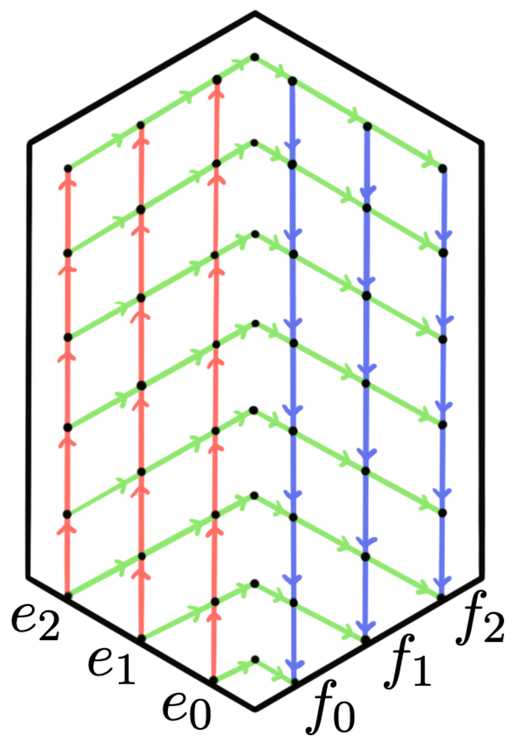
Note that any path $P_{i}$ crosses the $v_{3}$ -axis at a unique type $T_{3}$ tile $R_{k}$ with lowest point $kv_{3}$ for some $0\leq k\leq d+e$ . Every rhombic path from $e_{i}$ to $R_{k}$ consisting only of tiles of type $T_{2}$ and $T_{3}$ has length $k$ and contains exactly $i$ tiles of type $T_{3}$ . Hence there are $\binom{k}{i}$ such rhombic paths. Therefore, the $ik$ th entry of $M_{d,e}$ counts the number of rhombic paths from $e_{i}$ to $R_{k}$ , and by symmetry it follows that the $ij$ th entry of $M_{d,e}M_{d,e}^{T}$ counts the number of rhombic paths from $e_{i}$ to $f_{j}$ . Therefore the Lindström-Gessel-Viennot lemma [12, Cor. 2] applied to the acyclic digraph $G_{d,e}$ implies that $\delta(\Lambda_{d,e})=\det(M_{d,e}M_{d,e}^{T})=N(d+1,d+1,e)$ is the total number of non-crossing rhombic paths, hence the total number of plane partitions which fit inside a box of dimension $(d+1)\times(d+1)\times e$ . On the other hand, MacMahon’s theorem [21, p. 378] implies that

N(d+1,d+1,e)=\prod_{i=0}^{d}\prod_{j=1}^{e}\frac{d+i+j+1}{i+j}.\qed

Remark.

The use of the Lindström-Gessel-Viennot lemma to count plane partitions and to evaluate determinants of matrices with binomial coefficient entries is not new; however, we did not find the evaluation of $\delta(\Lambda_{d,e})$ among the known results. Many variations on this idea may be found in the literature (see, for example, [11, 12, 22]).

The following corollary extracts an upper bound on $\delta(\Lambda_{d,e})$ from the product formula in Theorem 2.1 that will be used in the proof of Theorem 2.5.

Corollary 2.2.

Let $d,e$ be integers such that $d\geq 33$ and $1\leq e\leq\log_{2}(d/2)$ . Then

(2.1)

\log_{2}(\delta(\Lambda_{d,e}))<2(d-1)\log_{2}(d/2)-e\log_{2}(d+e+1).

Proof.

Theorem 2.1 shows that $\delta(\Lambda_{d,e})$ is an increasing function of $e$ . Thus, it suffices to fix $e:=\lfloor\log_{2}(d/2)\rfloor$ and show that

(2.2)

\log_{2}(\delta(\Lambda_{d,e}))<2(d-1)e-e\log_{2}(d+e+1).

Taking the logarithm of the product formula

\delta(\Lambda_{d,e})=\prod_{i=0}^{d}\prod_{j=1}^{e}\frac{d+1+i+j}{i+j}

yields

	$\displaystyle\begin{split}\log_{2}(\delta(\Lambda_{d,e}))&=\sum_{i=0}^{d}\sum_{j=1}^{e}\log_{2}\left(\frac{d+1+i+j}{i+j}\right)\end{split}$
	$\displaystyle\begin{split}&=\sum_{n=1}^{d+e}\#\{(i,j):0\leq i\leq d,\ 1\leq j\leq e,\ i+j=n\}\cdot\log_{2}\left(\frac{d+1+n}{n}\right)\end{split}$
(2.3)		$\displaystyle\begin{split}&=\sum_{n=1}^{e}n\log_{2}\left(1+\frac{d+1}{n}\right)+\sum_{n=d+1}^{d+e}(d+e+1-n)\log_{2}\left(1+\frac{d+1}{n}\right)\\ &\qquad+e\sum_{n=e+1}^{d}\log_{2}\left(1+\frac{d+1}{n}\right).\end{split}$

Note that $\log_{2}\left(1+\frac{d+1}{n}\right)$ is a positive, decreasing function of $n$ . Hence,

\sum_{n=1}^{e}n\log_{2}\left(1+\frac{d+1}{n}\right)+\sum_{n=d+1}^{d+e}(d+e+1-n)\log_{2}\left(1+\frac{d+1}{n}\right)\leq\binom{e+1}{2}(\log_{2}(d+2)+1).

Note that for any $\varepsilon>0$ and for all sufficiently large $d$ (depending on $\varepsilon$ ),

	$\displaystyle\binom{e+1}{2}(\log_{2}(d+2)+1)$	$\displaystyle=\binom{e+1}{2}\log_{2}(d)+\binom{e+1}{2}\log_{2}\Big(1+\frac{2}{d}\Big)+\binom{e+1}{2}$
		$\displaystyle<\Big(\frac{1}{2}+\varepsilon\Big)e^{2}\log_{2}(d)+e^{2}.$

In particular, for if we take $\varepsilon=.03$ , then for all $d\geq 256$ we have

(2.4)

\sum_{n=1}^{e}n\log_{2}\left(1+\frac{d+1}{n}\right)+\sum_{n=d+1}^{d+e}(d+e+1-n)\log_{2}\left(1+\frac{d+1}{n}\right)<.53e^{2}\log_{2}(d)+e^{2}.

Interpreting the third sum in (2.3) as a right hand Riemann sum gives us

	$\displaystyle\sum_{n=e+1}^{d}\log_{2}\left(1+\frac{d+1}{n}\right)$	$\displaystyle\leq\int_{e}^{d}\log_{2}\Big(1+\frac{d+1}{x}\Big)\,dx$
		$\displaystyle=(2d+1)\log_{2}(2d+1)-d\log_{2}(d)-(d+e+1)\log_{2}(d+e+1)+e\log_{2}(e).$

Observe that for $d\geq 2$ ,

	$\displaystyle(2d+1)\log_{2}(2d+1)$	$\displaystyle=2d+1+(2d+1)\log_{2}(d)+(2d+1)\log_{2}\Big(1+\frac{1}{2d}\Big)$
		$\displaystyle\leq 2d+(2d+1)\log_{2}(d)+3,$

and

	$\displaystyle(d+e+1)\log_{2}(d+e+1)$	$\displaystyle=(d+e+1)\log_{2}(d)+(d+e+1)\log_{2}\Big(1+\frac{e+1}{d}\Big)$
		$\displaystyle\geq(d+e+1)\log_{2}(d)+e+1.$

Hence for $d\geq 2$ ,

	$\displaystyle\sum_{n=e+1}^{d}\log_{2}\left(1+\frac{d+1}{n}\right)$	$\displaystyle\leq 2d+(2d+1)\log_{2}(d)+3-d\log_{2}(d)$
		$\displaystyle\qquad-(d+e+1)\log_{2}(d)-e-1+e\log_{2}(e)$
(2.5)			$\displaystyle=2d-e\log_{2}(d)+e\log_{2}(e)-e+2.$

Combining the estimates (2.4) and (2.5) for $d\geq 256$ we have

	$\displaystyle\log_{2}(\delta(\Lambda_{d,e}))$	$\displaystyle<(2de-e^{2}\log_{2}(d)+e^{2}\log_{2}(e)-e^{2}+2e)+.53e^{2}\log_{2}(d)+e^{2}$
		$\displaystyle=2de-.47e^{2}\log_{2}(d)+e^{2}\log_{2}(e)+2e.$

It therefore suffices to prove that

2de-.47e^{2}\log_{2}(d)+e^{2}\log_{2}(e)+2e\leq 2(d-1)e-e\log_{2}(d+e+1),

which is equivalent to

(2.6)

e^{2}\log_{2}(e)+e\log_{2}(d+e+1)+4e\leq.47e^{2}\log_{2}(d),

which can be shown to hold for all $d\geq 1079$ . One may then check by computation that the inequality (2.1) holds for $33\leq d\leq 1079$ , completing the proof. ∎

Remark.

Cohen, Shpilka, and Tal [7, Lem. 6.4] proved, in our notation, that

\log_{2}(\delta(\Lambda_{d,e}))\leq(2d+e+1)e.

If $e\leq\log_{2}(d/2)$ , this gives the bound

(2.7)

\log_{2}(\delta(\Lambda_{d,e}))\leq 2d\log_{2}(d/2)+\log_{2}(d)^{2}-\log_{2}(d).

This bound has the same leading term as the bound we prove in Corollary 2.2, but the lower order terms in (2.7) do not suffice to prove Theorem 2.5.

2.2. Minkowski’s theorem on successive minima

Suppose that $K\subseteq\mathbb{R}^{m}$ is a compact, convex, centrally symmetric set. If $\Lambda\subseteq\mathbb{R}^{m}$ is a rank- $m$ lattice, then for $1\leq i\leq m$ the $i$ th successive minimum of $\Lambda$ with respect to $K$ , denoted $\lambda_{i}(\Lambda,K)$ , is defined by

\lambda_{i}(\Lambda,K):=\min\{r\in\mathbb{R}_{\geq 0}:\mathrm{span}(rK\cap\Lambda)\text{ has rank at least }i\}.

Note that the $\lambda_{i}(\Lambda,K)$ are positive and weakly increasing with $i$ . The following classical theorem of Minkowski relates the successive minima, the volume of $K$ , and the discriminant of $\Lambda$ . See [6, Chp. VIII, Thm. V].

Theorem 2.3 (Minkowski).

Let $m\geq 1$ , let $K\subseteq\mathbb{R}^{m}$ be a compact, convex, centrally symmetric set, and let $\Lambda\subseteq\mathbb{R}^{m}$ be a rank- $m$ lattice. Then

\mathrm{Vol}(K)\prod_{i=1}^{m}\lambda_{i}(\Lambda,K)\leq 2^{m}\sqrt{\delta(\Lambda)}.

Suppose that $K=[-1,1]^{m}\subseteq\mathbb{R}^{m}$ . Observe that, for $v\in\mathbb{R}^{m}$ and $r\geq 0$ , $v\in rK$ if and only if $||v||_{\infty}\leq r$ where

||(a_{1},a_{2},\ldots,a_{m})||_{\infty}:=\max_{i}|a_{i}|

is the usual max norm on $\mathbb{R}^{m}$ . We define $\lambda_{i}(\Lambda):=\lambda_{i}(\Lambda,[-1,1]^{m})$ . Since $\mathrm{Vol}([-1,1]^{m})=2^{m}$ , we have the following useful direct corollary of Theorem 2.3.

Corollary 2.4.

If $\Lambda\subseteq\mathbb{R}^{m}$ is a rank- $m$ lattice with discriminant $\delta(\Lambda)$ , then

\prod_{i=1}^{m}\lambda_{i}(\Lambda)\leq\sqrt{\delta(\Lambda)}.

2.3. Main Result

We now prove the first main result. Recall that for $d\geq 2$ ,

B_{d}:=\sup_{f}|\mathrm{PrePer}(f,\mathbb{Q})|\in[0,\infty],

where the supremum is taken over all $f(x)\in\mathbb{Q}[x]$ with $2\leq\deg(f)\leq d$ .

Theorem 2.5.

Let $d\geq 2$ be an integer. Then there exists a polynomial $f_{d}(x)\in\mathbb{Q}[x]$ with $2\leq\deg(f_{d})\leq d$ such that

f_{d}([d+\lfloor\log_{2}(d)\rfloor])\subseteq[d].

Hence for all $d\geq 2$ ,

B_{d}\geq d+\lfloor\log_{2}(d)\rfloor.

Proof.

Let $d\geq 2$ and $e\geq 0$ be integers. Recall the rank- $(d+1)$ lattice $\Lambda_{d,e}\subseteq\mathbb{R}^{d+e+1}$ constructed in Section 2.1 spanned by the $d+1$ vectors

u_{i}:=\left(\binom{0}{i},\binom{1}{i},\ldots,\binom{d+e}{i}\right)\in\mathbb{Z}^{d+e+1}

for $0\leq i\leq d$ . Let $M$ be a real number such that $M>\frac{d\sqrt{d+e+1}}{2}$ and let $v_{1},v_{2},\ldots,v_{e}$ be an orthogonal basis for the orthogonal complement of $\Lambda_{d,e}$ in $\mathbb{R}^{d+e+1}$ such that $||v_{j}||=M$ for all $j$ . Define $\widetilde{\Lambda}_{d,e}$ to be the rank- $(d+e+1)$ lattice spanned by the $u_{i}$ and $v_{j}$ with $0\leq i\leq d$ and $1\leq j\leq e$ . Note that for any vector $w\in\widetilde{\Lambda}_{d,e}$ supported on some $v_{j}$ we have

(2.8)

||w||_{\infty}\geq\frac{||w||}{\sqrt{d+e+1}}\geq\frac{||v_{j}||}{\sqrt{d+e+1}}=\frac{M}{\sqrt{d+e+1}}>\frac{d}{2}.

We claim that for $d\geq 33$ and $e:=\lfloor\log_{2}(d/2)\rfloor=\lfloor\log_{2}(d)\rfloor-1$ we have

(2.9)

\lambda_{3}(\widetilde{\Lambda}_{d,e})<\frac{d}{2}.

First we finish the proof of the theorem assuming (2.9), and then we return to prove the claim.

If (2.9) holds, then there are three linearly independent vectors $w_{1},w_{2},w_{3}\in\widetilde{\Lambda}_{d,e}$ such that $||w_{i}||_{\infty}<\frac{d}{2}$ . Thus (2.8) implies that each $w_{i}$ is supported only on the $u_{j}$ with $0\leq j\leq d$ . Linear independence implies that at least one $w_{i}$ must be supported on a $u_{j}$ with $j\geq 2$ . Suppose without loss of generality that $w_{1}=\sum_{i=0}^{d}a_{i}u_{i}$ where $a_{i}\in\mathbb{Z}$ and $a_{i}\neq 0$ for some $i\geq 2$ . If $g(x):=\sum_{i=0}^{d}a_{i}\binom{x}{i}$ , then $w_{1}=(g(0),g(1),\ldots,g(d+e))$ . Hence $|g(i)|\leq||w_{1}||_{\infty}<d/2$ for $0\leq i\leq d+e$ . Note that $g(x)$ is an integer-valued polynomial. Thus $f_{d}(x):=g(x-1)+\lfloor d/2\rfloor+1$ is an integer-valued polynomial with $2\leq\deg(f_{d})\leq d$ such that for all $i\in[d+e+1]=[d+\lfloor\log_{2}(d)\rfloor]$ ,

0\leq\lfloor d/2\rfloor-d/2+1<f_{d}(i)<\lfloor d/2\rfloor+d/2+1\leq d+1.

Therefore $f_{d}([d+\lfloor\log_{2}(d)\rfloor])\subseteq[d]$ , as we wished to show.

Now we turn to proving (2.9). By construction, we have

\delta(\widetilde{\Lambda}_{d,e})=\delta(\Lambda_{d,e})M^{2e}.

If $i>d+1$ , then any set of $i$ independent vectors in $\widetilde{\Lambda}_{d,e}$ must contain at least one vector $w$ supported on some $v_{j}$ . Hence $||w||_{\infty}\geq M/\sqrt{d+e+1}$ by (2.8). Thus for $i>d+1$ ,

\lambda_{i}(\widetilde{\Lambda}_{d,e})\geq\frac{M}{\sqrt{d+e+1}}>\frac{d}{2}.

The vectors $u_{i}$ all have integer entries, hence $\lambda_{1}(\widetilde{\Lambda}_{d,e})\geq 1$ . The monotonicity of the $\lambda_{i}(\widetilde{\Lambda}_{d,e})$ gives us

\prod_{i=1}^{d+e+1}\lambda_{i}(\widetilde{\Lambda}_{d,e})\geq\lambda_{3}(\widetilde{\Lambda}_{d,e})^{d-1}\Big(\frac{M}{\sqrt{d+e+1}}\Big)^{e}.

Therefore, Corollary 2.4 implies that

\lambda_{3}(\widetilde{\Lambda}_{d,e})^{d-1}\Big(\frac{M}{\sqrt{d+e+1}}\Big)^{e}\leq\prod_{i=1}^{d+e+1}\lambda_{i}(\widetilde{\Lambda}_{d,e})\leq\sqrt{\delta(\widetilde{\Lambda}_{d,e})}=\sqrt{\delta(\Lambda_{d,e})}\cdot M^{e},

from which we conclude that

\log_{2}(\lambda_{3}(\widetilde{\Lambda}_{d,e}))\leq\frac{\log_{2}(\delta(\Lambda_{d,e}))+e\log_{2}(d+e+1)}{2(d-1)}.

Corollary 2.2 implies that

\log_{2}(\delta(\Lambda_{d,e}))<2(d-1)\log_{2}(d/2)-e\log_{2}(d+e+1)

for $d\geq 33$ , hence

\log_{2}(\lambda_{3}(\widetilde{\Lambda}_{d,e}))<\log_{2}(d/2),

which is equivalent to (2.9).

Now suppose that $2\leq d\leq 32$ . If $2\leq d\leq 7$ , then $\lfloor\log_{2}(d/2)\rfloor\leq 1$ . Lagrange interpolation immediately implies the existence of polynomials $f_{d}(x)\in\mathbb{Q}[x]$ with degree $d$ such that $f_{d}([d+1])\subseteq[d]$ . If $8\leq d\leq 32$ , then $\log_{2}(d/2)\leq 4$ and the sequence of polynomials $t_{d}(x)$ constructed in Corollary 4.3 satisfies

t_{d}([d+4])\subseteq[5]\subseteq[d],

which suffices to complete the proof. ∎

Remark.

The idea of augmenting the lattice $\Lambda_{d,e}$ by arbitrary long vectors is borrowed from the proof of [7, Theorem 1.5]. This strategy greatly simplifies our original approach.

3. Common preperiodic points

In this section we prove Proposition 1.8 and part of Corollary 1.4(2), restated as Proposition 3.2 and Theorem 3.4 below.

Lemma 3.1.

If $f(x)\in\mathbb{C}[x]$ is a degree- $d$ polynomial and $S\subseteq\mathbb{C}$ is a set with $n$ elements, then

|f^{-1}(S)|\geq dn-d+1.

Proof.

Let $e_{p}$ denote the ramification index of $f(x)$ at $p\in\mathbb{C}$ . Then for all $q\in\mathbb{C}$ ,

d=\sum_{p\in f^{-1}(q)}e_{p}=|f^{-1}(q)|+\sum_{p\in f^{-1}(q)}(e_{p}-1).

A point $p\in\mathbb{C}$ has $e_{p}>1$ if and only if $p$ is a root of $f^{\prime}(x)$ with multiplicity $e_{p}-1$ , hence

d-1=\sum_{p\in\mathbb{C}}(e_{p}-1).

Thus,

|f^{-1}(S)|=\sum_{q\in S}|f^{-1}(q)|=dn-\sum_{p\in f^{-1}(S)}(e_{p}-1)\geq dn-d+1.\qed

Proposition 3.2.

Suppose that $f(x)\in\mathbb{Q}[x]$ is a degree $d\geq 2$ polynomial such that

f([m])\subseteq[n]

for some integers $m>n\geq 0$ . Then

(1)

$f^{-1}([n])\subseteq\bigcap_{i=0}^{m-n}\mathrm{PrePer}(f(x)+i,\mathbb{C})$ ,
(2)

$|f^{-1}([n])|\geq dn-d+1$ , and
(3)

$\mathrm{PrePer}(f(x)+i,\mathbb{C})\neq\mathrm{PrePer}(f(x)+j,\mathbb{C})$ for all $0\leq i<j\leq m-n$ .

Hence

d(n-1)+1\leq\left|\bigcap_{i=0}^{m-n}\mathrm{PrePer}(f(x)+i,\mathbb{C})\right|<\infty.

Proof.

Let $0\leq i\leq m-n$ . If $f([m])\subseteq[n]$ , then

f(f^{-1}([n]))+i\subseteq[n+i]\subseteq[m]\subseteq f^{-1}([n]).

Hence $f^{-1}([n])\subseteq\mathrm{PrePer}(f(x)+i,\mathbb{C})$ , proving (1). The lower bound $|f^{-1}([n])|\geq dn-d+1$ follows immediately from Lemma 3.1 since $[n]$ contains $n$ points.

For (3) it suffices to prove that for any polynomial $h(x)$ and any positive integer $i$ , $\mathrm{PrePer}(h(x),\mathbb{C})\neq\mathrm{PrePer}(h(x)+i,\mathbb{C})$ . Since $h(x)$ is a polynomial, $\infty$ is a superattracting fixed point, and thus the set $\mathrm{PrePer}(h(x),\mathbb{C})$ of finite complex preperiodic points of $h(x)$ is bounded. Therefore, there exists some $q\in\mathrm{PrePer}(h(x),\mathbb{C})$ such that $q+i\not\in\mathrm{PrePer}(h(x),\mathbb{C})$ . Let $p\in h^{-1}(q)$ . Then $p\in\mathrm{PrePer}(h(x),\mathbb{C})$ by construction. If $p\in\mathrm{PrePer}(h(x)+i,\mathbb{C})$ , then $h(p)+i=q+i\in\mathrm{PrePer}(h(x)+i,\mathbb{C})\setminus\mathrm{PrePer}(h(x),\mathbb{C})$ . Otherwise, $p\in\mathrm{PrePer}(h(x),\mathbb{C})\setminus\mathrm{PrePer}(h(x)+i,\mathbb{C})$ . In either case, we have $\mathrm{PrePer}(h(x),\mathbb{C})\neq\mathrm{PrePer}(h(x)+i,\mathbb{C})$ .

Finally, Baker and DeMarco [1, Thm. 1.2] proved that if $f(x),g(x)\in\mathbb{C}(x)$ are rational functions of degree at least 2, then $\mathrm{PrePer}(f(x),\mathbb{C})\neq\mathrm{PrePer}(g(x),\mathbb{C})$ implies $\mathrm{PrePer}(f(x),\mathbb{C})\cap\mathrm{PrePer}(g(x),\mathbb{C})$ is finite. Therefore,

d(n-1)+1\leq\Big|\bigcap_{i=0}^{m-n}\mathrm{PrePer}(f(x)+i,\mathbb{C})\Big|<\infty.\qed

Example 3.3.

Consider the degree-6 polynomial

f(x)=\frac{x^{6}-45x^{5}+775x^{4}-6375x^{3}+25504x^{2}-45060x+30960}{720}.

One may check that

f([14])\subseteq[10].

Therefore Proposition 3.2 implies that $\bigcap_{i=0}^{4}\mathrm{PrePer}(f(x)+i,\mathbb{C})$ is finite and contains at least 55 points.

Recall that $C_{d}$ for $d\geq 2$ is defined by

C_{d}:=\sup_{f,g}|\mathrm{PrePer}(f,\mathbb{C})\cap\mathrm{PrePer}(g,\mathbb{C})|,

where the supremum is taken over all $f(x),g(x)\in\mathbb{C}[x]$ with $2\leq\deg(f),\deg(g)\leq d$ such that $\mathrm{PrePer}(f,\mathbb{C})\neq\mathrm{PrePer}(g,\mathbb{C})$ .

Theorem 3.4.

Let $d\geq 2$ be an integer. There exists a polynomial $f_{d}(x)\in\mathbb{Q}[x]$ with $2\leq\deg(f_{d})\leq d$ such that

\Big|\mathrm{PrePer}(f_{d}(x)+i,\mathbb{C})\cap\mathrm{PrePer}(f_{d}(x)+j,\mathbb{C})\Big|<\infty\text{ for all $0\leq i<j\leq\log_{2}(d)$}

and

(3.1)

\Big|\bigcap_{i=0}^{\lfloor\log_{2}(d)\rfloor}\mathrm{PrePer}(f_{d}(x)+i,\mathbb{C})\Big|\geq\deg(f_{d})(d-1)+1.

Furthermore, there exist infinitely many $d$ such that

(3.2)

C_{d}\geq d^{2}+d\lfloor\log_{2}(d)\rfloor-2d+1.

Proof.

Theorem 2.5 implies that for $d\geq 2$ there exists a polynomial $f_{d}(x)\in\mathbb{Q}[x]$ with $2\leq\deg(f_{d})\leq d$ such that

f_{d}([d+\lfloor\log_{2}(d)\rfloor])\subseteq[d].

Hence (3.1) follows from Proposition 3.2.

Let $e_{d}:=\lfloor\log_{2}(d)\rfloor$ , then

f_{d}([d+e_{d}])\subseteq[d]\subseteq[d+e_{d}-1].

Hence applying Proposition 3.2 with $m=d+e_{d}$ and $n=d+e_{d}-1$ , we have

\deg(f_{d})(d+e_{d}-2)+1\leq|\mathrm{PrePer}(f_{d}(x),\mathbb{C})\cap\mathrm{PrePer}(f_{d}(x)+1,\mathbb{C})|<\infty.

Cohen, Shpilka, and Tal [7, Cor. 1.2] prove that for all $m$ sufficiently large, if $f(x)\in\mathbb{Q}[x]$ is a polynomial with $\deg(f)\geq 2$ such that $f([m])\subseteq[m-1]$ , then

\deg(f)\geq m\Big(1-\frac{4}{\log_{2}\log_{2}(m)}\Big).

Hence, for all $d$ sufficiently large,

\deg(f_{d})\geq(d+e_{d})\Big(1-\frac{4}{\log_{2}\log_{2}(d+e_{d})}\Big)\geq d\Big(1-\frac{4}{\log_{2}\log_{2}(d)}\Big).

Note that the quantity on the right-hand side tends to $\infty$ with $d$ ; thus, the same is true for $\deg(f_{d})$ .

Now, let $d^{\prime}\geq 2$ , and let $d:=\deg f_{d^{\prime}}\leq d^{\prime}$ . By the conclusion of the previous paragraph, there are infinitely many integers $d$ arising in this way. In this case, we have

C_{d}\geq d(d^{\prime}+\lfloor\log_{2}(d)\rfloor-2)+1\geq d^{2}+d\lfloor\log_{2}(d)\rfloor-2d+1.

Thus (3.2) holds for infinitely many $d$ . ∎

4. Examples of exceptional preperiodic behavior in every degree

In Theorem 2.5 we showed that for all sufficiently large degrees $d$ , there exists a degree-at-most- $d$ polynomial with at least $d+\lfloor\log_{2}(d)\rfloor$ rational preperiodic points. However, the proof is not constructive, in the sense that it does not allow us to provide an explicit formula for such a polynomial. In this section we construct a family of polynomials $r_{d}(x)\in\mathbb{Q}[x]$ such that, for all $d\geq 2$ , $r_{d}$ is a degree- $d$ polynomial with at least $d+6$ rational preperiodic points. For $d<64$ , this improves the lower bound on $B_{d}$ obtained from Theorem 2.5.

First we introduce a doubly periodic sequence $\rho(m,d)$ and use its values to interpolate an auxiliary sequence of polynomials $s_{d}(x)$ .

Lemma 4.1.

There is a unique function $\rho:\mathbb{Z}^{2}\to\mathbb{Z}$ satisfying the following properties:

(i)

$\rho(m+3,d)=-\rho(m,d)$ for all $(m,d)\in\mathbb{Z}^{2}$ ,
(ii)

$\rho(m,d+1)=-\rho(m+1,d)$ for all $(m,d)\in\mathbb{Z}^{2}$ , and
(iii)

$\rho(0,0)=\rho(1,0)=1$ , and $\rho(2,0)=0$ .

Furthermore, for all $(m,d)\in\mathbb{Z}^{2}$ ,

(1)

$\rho(m,d+3)=\rho(m,d)$ ,
(2)

$\rho(m+1,d+1)=\rho(m,d)+\rho(m,d+1)$ ,
(3)

$\rho(m,d)=(-1)^{d}\rho(d+1-m,d)$ .

Proof.

The initial values together with (i) imply that $\rho(m,0)$ is well-defined for all $m\in\mathbb{Z}$ . Then (ii) implies that $\rho(m,d)=(-1)^{d}\rho(m+d,0)$ . Hence these three properties uniquely determine $\rho(m,d)$ for all $(m,d)\in\mathbb{Z}^{2}$ .

$m$	0	1	2	3	4	5
$\rho(m,0)$	1	1	0	$-1$	$-1$	0

Table 1. Initial values that determine

\rho(m,n)

(1) Properties (i) and (ii) imply that

\rho(m,d+3)=(-1)^{3}\rho(m+3,d)=-\rho(m+3,d)=\rho(m,d).

(2) Since $\rho(m+6,d)=\rho(m,d)$ , we can check the following identity by inspection:

\rho(m+2,0)=\rho(m+1,0)-\rho(m,0).

Replacing $m$ by $m+d$ yields

\rho((m+1)+(d+1),0)=\rho(m+(d+1),0)-\rho(m+d,0),

and repeatedly applying (ii) gives

(-1)^{d+1}\rho(m+1,d+1)=(-1)^{d+1}\rho(m,d+1)+(-1)^{d+1}\rho(m,d);

dividing by $(-1)^{d+1}$ yields (2).

(3) Using $\rho(m+6,d)=\rho(m,d)$ we may verify that for all $m\in\mathbb{Z}$ ,

(4.1)

\rho(m,0)=\rho(1-m,0).

Thus, if $d=2n$ is even, then

\rho(m,2n)=\rho(m+2n,0)=\rho(m-4n,0)=\rho(4n+1-m,0)=\rho(2n+1-m,2n).

Similarly, if $d=2n+1$ is odd, then (4.1) implies that

\rho(m,2n+1)=-\rho(m+2n+1,0)=-\rho(m-4n+1,0)=-\rho(4n-m,0)=\rho(2n-1-m,2n+1).

Finally, (i) implies

\rho(2n-1-m,2n+1)=-\rho(2n+2-m,2n+1).

Hence in either case,

\rho(m,d)=(-1)^{d}\rho(d+1-m,d).\qed

Let $s_{d}(x)\in\mathbb{Q}[x]$ be the unique degree-at-most- $d$ polynomial such that

s_{d}(m-\tfrac{d+1}{2})=\rho(m,d),

for $0\leq m\leq d$ . Lemma 4.2 establishes some basic properties of $s_{d}(x)$ . Let $\delta$ denote the centered difference operator defined by

\delta f(x):=f(x+\tfrac{1}{2})-f(x-\tfrac{1}{2}).

Lemma 4.2.

Let $d\geq 0$ .

(1)

$s_{d}(-x)=(-1)^{d}s_{d}(x)$ ,
(2)

$\delta s_{d+1}(x)=s_{d}(x)$ ,
(3)

$\deg(s_{d})=d$ ,
(4)

$s_{d}(d+1-\tfrac{d+1}{2})=\rho(d+1,d)$ ,
(5)

$s_{d}(d+2-\tfrac{d+1}{2})=\rho(d+2,d)+1$ ,
(6)

$s_{d}(d+3-\tfrac{d+1}{2})=\rho(d+3,d)+d+2$ .

Proof.

(1) Suppose $f(x)\in\mathbb{R}[x]$ is a degree-at-most- $d$ polynomial. Then $f(x)-(-1)^{d}f(-x)$ has degree at most $d-1$ . Hence if there are at least $\lfloor\tfrac{d+1}{2}\rfloor$ distinct pairs $\pm a$ of real numbers for which $f(a)=(-1)^{d}f(-a)$ , then it follows that the identity $f(x)=(-1)^{d}f(-x)$ holds in $\mathbb{R}[x]$ .

Lemma 4.1(3) implies that for $1\leq m\leq d$ ,

s_{d}(m-\tfrac{d+1}{2})=\rho(m,d)=(-1)^{d}\rho(d+1-m,d)=(-1)^{d}s_{d}(d+1-m-\tfrac{d+1}{2})=(-1)^{d}s_{d}(\tfrac{d+1}{2}-m),

since $1\leq m\leq d$ is equivalent to $1\leq d+1-m\leq d$ . The set $\{m-\tfrac{d+1}{2}:1\leq m\leq d\}$ contains at least $\lfloor\tfrac{d+1}{2}\rfloor$ pairs $\pm a$ , hence it follows that $s_{d}(x)=(-1)^{d}s_{d}(-x)$ for all $d\geq 0$ .

(2) Let $f(x)$ be the degree-at-most- $d$ polynomial

f(x):=\det s_{d+1}(x)=s_{d+1}(x+\tfrac{1}{2})-s_{d+1}(x-\tfrac{1}{2}).

If $0\leq m\leq d$ , then by Lemma 4.1(2),

	$\displaystyle f(m-\tfrac{d+1}{2})$	$\displaystyle=s_{d+1}(m+1-\tfrac{d+2}{2})-s_{d+1}(m-\tfrac{d+2}{2})$
		$\displaystyle=\rho(m+1,d+1)-\rho(m,d+1)$
		$\displaystyle=\rho(m,d)$
		$\displaystyle=s_{d}(m-\tfrac{d+1}{2}).$

Hence $f(x)=s_{d}(x)$ .

(3) If $f(x)$ has degree $d\geq 1$ , then $\delta f(x)$ has degree $d-1$ . Since $s_{0}(x)=1$ has degree 0 by construction, it follows from (2) that $\deg(s_{d})=d$ for all $d\geq 0$ .

(4) By (1) and Lemma 4.1(3),

s_{d}(d+1-\tfrac{d+1}{2})=(-1)^{d}s_{d}(0-\tfrac{d+1}{2})=(-1)^{d}\rho(0,d)=\rho(d+1,d).

(5) We prove this identity by induction on $d$ . Since $s_{0}(x)=1$ is constant,

s_{0}(0+2-\tfrac{0+1}{2})=1=\rho(2,0)+1.

Now let $d\geq 1$ and suppose that the identity (5) holds for $d-1$ . By (2), (4), and Lemma 4.1(2),

	$\displaystyle s_{d}(d+2-\tfrac{d+1}{2})$	$\displaystyle=s_{d}(d+1-\tfrac{d+1}{2})+s_{d-1}(d+1-\tfrac{d}{2})$
		$\displaystyle=\rho(d+1,d)+\rho(d+1,d-1)+1$
		$\displaystyle=\rho(d+2,d)+1.$

(6) Following the induction in (5) we first observe that

s_{0}(0+3-\tfrac{0+1}{2})=1=\rho(3,0)+0+2.

If $d\geq 1$ and we suppose that (6) holds for $d-1$ , then by (2), (5), and Lemma 4.1(2),

	$\displaystyle s_{d}(d+3-\tfrac{d+1}{2})$	$\displaystyle=s_{d}(d+2-\tfrac{d+1}{2})+s_{d-1}(d+2-\tfrac{d}{2})$
		$\displaystyle=\rho(d+2,d)+1+\rho(d+2,d-1)+d-1+2$
		$\displaystyle=\rho(d+3,d)+d+2.\qed$

After a change of coordinates, the polynomials $s_{d}(x)$ provide explicit examples of a family of polynomial that compress many consecutive integers into an interval of fixed length. These examples cover the low degree cases needed to complete the proof of Theorem 2.5.

Corollary 4.3.

For $d\geq 0$ let $t_{d}(x)\in\mathbb{Q}[x]$ be the degree $d$ polynomial defined by

t_{d}(x):=s_{d}(x-2-\tfrac{d+1}{2})+3.

Then

t_{d}([d+4])\subseteq[5].

Proof.

Lemma 4.2 and the definition of $s_{d}(x)$ implies that $s_{d}(m-\tfrac{d+1}{2})\in[-2,2]\cap\mathbb{Z}$ for all integers $m$ such that $-2\leq m\leq d+2$ . Hence it follows that $t_{d}([d+4])\subseteq[5]$ . ∎

4.1. Constructing $r_{d}(x)$

For $d\geq 0$ , let $r_{d}(x)\in\mathbb{Q}[x]$ be the polynomial sequence defined by

r_{d}(x):=\begin{cases}s_{d}(x-3-\tfrac{d+1}{2})+2&\text{if $d$ is even,}\\ s_{d}(x-3-\tfrac{d+1}{2})-x+d+6&\text{if $d$ is odd.}\end{cases}

Theorem 4.4.

For all $d\geq 2$ , $r_{d}(x)$ is a degree- $d$ , integer-valued polynomial such that if $d$ is even, then

r_{d}([d+6])\subseteq[d+5],

and if $d$ is odd, then

r_{d}([d+6])\subseteq[d+4].

Thus,

(1)

$B_{d}\geq d+6$ for all $d\geq 2$ , and
(2)

$C_{d}\geq d^{2}+4d+1$ for all $d\geq 2$ .

Proof.

Lemma 4.2(3) implies that $r_{d}(x)$ has degree $d$ , and the fact that $s_{d}(y-\frac{d+1}{2})$ is an integer for all $0\leq y\leq d$ , and therefore $r_{d}(x)$ is an integer for all $3\leq x\leq d+3$ , implies that $r_{d}$ is integer-valued for all $d\geq 0$ .

Suppose that $d\geq 2$ is even. If $3\leq k\leq d+4$ , then the definition of $s_{d}(x)$ and Lemma 4.2(4) gives us,

r_{d}(k)=s_{d}(k-3-\tfrac{d+1}{2})+2=\rho(k-3,d)+2\in[1,3].

From $s_{d}(x)$ even we find that

r_{d}(d+7-x)=s_{d}(\tfrac{d+7}{2}-x)+2=s_{d}(x-\tfrac{d+7}{2})+2=r_{d}(x).

Hence by Lemma 4.2(5) and (6),

	$\displaystyle r_{d}(1)$	$\displaystyle=r_{d}(d+6)=s_{d}(d+3-\tfrac{d+1}{2})+2=\rho(d+3,d)+d+4\in[d+3,d+5],$
	$\displaystyle r_{d}(2)$	$\displaystyle=r_{d}(d+5)=s_{d}(d+2-\tfrac{d+1}{2})+2=\rho(d+2,d)+3\in[2,4].$

Thus if $d$ is even,

r_{d}([d+6])\subseteq[d+5],

from which it follows that $B_{d}\geq|\mathrm{PrePer}(r_{d}(x),\mathbb{Q})|\geq d+6$ .

Next suppose that $d\geq 2$ is odd. If $3\leq k\leq d+4$ , then as above we have

r_{d}(k)=s_{d}(k-3-\tfrac{d+1}{2})-k+d+6=\rho(k-3,d)-k+d+6\in[1,d+4].

Lemma 4.2(5) and (6) gives us

	$\displaystyle r_{d}(d+5)$	$\displaystyle=s_{d}(d+2-\tfrac{d+1}{2})+1=\rho(d+2,d)+2\in[1,3],$
	$\displaystyle r_{d}(d+6)$	$\displaystyle=s_{d}(d+3-\tfrac{d+1}{2})=\rho(d+3,d)+d+2\in[d+1,d+3].$

Since $s_{d}(x)$ is odd,

	$\displaystyle d+5-r_{d}(d+7-x)$	$\displaystyle=d+5-s_{d}((d+7-x)-3-\tfrac{d+1}{2})+(d+7-x)-d-6$
		$\displaystyle=-s_{d}(-x+3+\tfrac{d+1}{2})-x+d+6$
		$\displaystyle=s_{d}(x-3-\tfrac{d+1}{2})-x+d+6$
		$\displaystyle=r_{d}(x).$

Thus,

	$\displaystyle r_{d}(1)$	$\displaystyle=d+5-r_{d}(d+6)\in[2,4]$
	$\displaystyle r_{d}(2)$	$\displaystyle=d+5-r_{d}(d+5)\in[d+2,d+4].$

Therefore,

r_{d}([d+6])\subseteq[d+4],

and it follows that $B_{d}\geq d+6$ for all $d\geq 2$ . Since for either parity of $d$ we have

r_{d}([d+6])\subseteq[d+5],

Proposition 3.2 implies that for all $d\geq 2$ ,

|\mathrm{PrePer}(r_{d}(x),\mathbb{C})\cap\mathrm{PrePer}(r_{d}(x)+1,\mathbb{C})|\geq d(d+4)+1=d^{2}+4d+1.

Hence $C_{d}\geq d^{2}+4d+1$ for all $d\geq 2$ . ∎

Figure 9 illustrates the typical behavior of the polynomials $r_{d}(x)$ in the interval $[1,d+6]$ .

Figure 9. The graphs of

r_{12}(x)

and

r_{13}(x)

4.2. Explicit formulas for $s_{d}(x)$

We suspect there is more of interest to say about the dynamical properties of the sequence of polynomials $r_{d}(x)$ . Thus to facilitate their future study we end this section by deriving explicit formulas for the polynomials $s_{d}(x)$ , which then allow for direct calculation of $r_{d}(x)$ .

For $d\geq 0$ , let $c_{d}(x)\in\mathbb{Q}[x]$ be the polynomial sequence defined by

c_{2k}(x):=\frac{1}{(2k)!}\prod_{j=1}^{k}\left(x^{2}-\tfrac{(2j-1)^{2}}{4}\right)\hskip 54.2025ptc_{2k+1}(x):=\frac{1}{(2k+1)!}x\prod_{j=1}^{k}(x^{2}-j^{2}).

Note that, by construction, $c_{d}(x)$ is even when $d$ is even and $c_{d}(x)$ is odd when $d$ is odd. A straightforward comparison of roots and leading coefficients implies that

\delta c_{d+1}(x)=c_{d}(x)

for $d\geq 0$ , and $\delta c_{0}(x)=\delta\,1=0$ . Furthermore, $c_{2k}(x)$ is integer-valued on $\mathbb{Z}+\tfrac{1}{2}$ and $c_{2k+1}(x)$ is integer-valued on $\mathbb{Z}$ .

Proposition 4.5.

For all $k\geq 0$ ,

s_{2k}(x):=\sum_{j=0}^{k}(-1)^{k-j}c_{2j}(x)\qquad\text{and}\qquad s_{2k+1}(x):=\sum_{j=0}^{k}(-1)^{k-j}c_{2j+1}(x).

Proof.

First observe that $\{c_{2k}:k\geq 0\}$ forms a basis for the vector space of even polynomials in $\mathbb{Q}[x]$ . Therefore there are rational numbers $\alpha_{j}$ such that

s_{2k}(x):=\sum_{j=0}^{k}\alpha_{j}c_{2j}(x).

Since

c_{2k}(\tfrac{1}{2})=\begin{cases}1&\text{if $k=0$,}\\ 0&\text{otherwise,}\end{cases}

it follows from Lemma 4.1 and Lemma 4.2 that

\alpha_{j}=\delta^{2j}s_{2k}(\tfrac{1}{2})=s_{2(k-j)}(\tfrac{1}{2})=\rho(k-j,2(k-j))=\rho(3(k-j),0)=(-1)^{k-j}\rho(0,0)=(-1)^{k-j}.

The expansion for $s_{2k+1}(x)$ follows by applying $\delta$ to the expansion of $s_{2k+2}(x)$ . ∎

5. Low degree examples

In this final section we provide lower bounds for $B_{d}$ and $C_{d}$ in low degrees found by computation. Table 2 gives examples of polynomials $f(x)$ and integers $m,n$ such that

(5.1)

f([m])\subseteq[n].

These are the polynomials with the largest $m$ for each degree $d$ that we found by computer search. Thus the entries in the column labeled $m$ also provide the best known lower bounds on $B_{d}$ for $2\leq d\leq 9$ .

$d$	$m$	$n$	$f(x)$
2	8	7	${\scriptstyle\frac{x^{2}-9x+22}{2}}$
3	11	11	${\scriptstyle\frac{x^{3}-18x^{2}+89x-66}{6}}$
4	10	8	${\scriptstyle\frac{x^{4}-22x^{3}+167x^{2}-506x+552}{24}}$
5	13	9	${\scriptstyle\frac{x^{5}-35x^{4}+445x^{3}-2485x^{2}+5794x-3600}{120}}$
6	14	10	${\scriptstyle\frac{x^{6}-45x^{5}+775x^{4}-6375x^{3}+25504x^{2}-45060x+30960}{720}}$
7	15	15	${\scriptstyle\frac{x^{7}-56x^{6}+1246x^{5}-14000x^{4}+83629x^{3}-258104x^{2}+373764x-151200}{5040}}$
8	16	16	${\scriptstyle\frac{x^{8}-68x^{7}+1918x^{6}-29036x^{5}+254989x^{4}-1309952x^{3}+3765012x^{2}-5343984x+2862720}{20160}}$
8	16	15	${\scriptstyle\frac{x^{8}-68x^{7}+1946x^{6}-30464x^{5}+282569x^{4}-1559852x^{3}+4836124x^{2}-7320336x+4273920}{40320}}$
9	19	17	${\scriptstyle\frac{x^{9}-90x^{8}+3426x^{7}-71820x^{6}+904449x^{5}-7002450x^{4}+32752124x^{3}-87183720x^{2}+116300160x-55520640}{181440}}$

Table 2.

One fast method to find these examples in low degree is to use the LLL basis reduction algorithm to find short vectors in the lattice $\Lambda_{d,e}$ defined in Section 2.1. Using this method we surveyed up to degree $d=400$ and found examples giving $B_{d}\geq d+8$ for all $11\leq d\leq 283$ except for

d\in\{21,219,221,235,237,241,244,\ldots,247,249,251,255,\ldots,266,268,269,271\}.

For all other degrees $11\leq d\leq 400$ the examples showed that $B_{d}\geq d+6$ , which we already knew by Theorem 4.4.

When $n<m$ in Table 2, Proposition 3.2 applied to $f([m])\subseteq[m-1]$ allows us to extract lower bounds on $C_{d}$ . Note that the lower bound on $C_{2}$ in Table 3 comes from Example 1.9.

In Table 3 we collect the best lower bounds on $C_{d}$ for small $d$ that we found through computational experiment. All of our examples came from common preperiodic points of $f(x)$ and $f(x)+1$ for some polynomial $f(x)$ exhibiting dynamical compression.

$d$	2	3	4	5	6	7	8	9	10	11	12	13	14	15
$C_{d}\geq$	26	27	40	60	78	84	120	162	190	198	228	260	294	330

Table 3.

For degrees $d=2,4,5,6,8,9$ , the polynomials giving the lower bound on $C_{d}$ come from Table 2. For degrees $d=3,7$ , the polynomials $r_{d}(x)$ constructed in Section 4.1 give the lower bound. For $10\leq d\leq 15$ , the polynomials $f_{d}(x)$ giving the lower bounds on $C_{d}$ are too large to print explicitly. Instead, Table 4 lists $d+1$ interpolating values $(f_{d}(1),f_{d}(2),\ldots,f_{d}(d+1))$ which uniquely determine the polynomial $f_{d}(x)$ .

$d$	$(f_{d}(1),f_{d}(2),\ldots,f_{d}(d+1))$
10	(14, 6, 14, 6, 1, 6, 14, 17, 14, 10, 10)
11	(17, 1, 15, 3, 4, 14, 17, 12, 8, 9, 10, 6)
12	(17, 1, 17, 3, 4, 14, 17, 12, 6, 3, 3, 6, 12)
13	(17, 1, 17, 1, 3, 13, 16, 13, 10, 9, 9, 9, 8, 5)
14	(20, 4, 20, 4, 20, 14, 1, 8, 21, 18, 6, 6, 18, 21, 8)
15	(21, 1, 2, 20, 4, 1, 9, 10, 5, 3, 6, 11, 16, 19, 17, 12)

Table 4.

References

[1] M. Baker, L. DeMarco, Preperiodic points and unlikely intersections, Duke Math. J., 159, no. 11 (2011), DOI: 10.1215/00127094-1384773.
[2] R. L. Benedetto, B. Dickman, S. Joseph, B. Krause, D. Rubin, X. Zhou, Computing points of small height for cubic polynomials, Involve, 2, no. 1 (2009), 37–64.
[3] T. Blum, J. R. Doyle, T. Hyde, C. Kelln, H. Talbott, M. Weinreich, Dynamical moduli spaces and polynomial endomorphisms of configurations, Arnold Math. J., to appear.
[4] P. Cahen, J. Chabert, Integer-Valued Polynomials, Mathematical Surveys and Monographs, 48, American Mathematical Society (1997).
[5] L. Caporaso, J. Harris, B. Mazur, How many rational points can a curve have?, The Moduli Space of Curves, Progress in Mathematics, 129, Birkhäuser Boston (1995).
[6] J. W. S. Cassels, An introduction to the geometry of numbers, Classics in Mathematics, 99, Springer Science & Business Media (1971).
[7] G. Cohen, A. Shpilka, A. Tal, On the degree of univariate polynomials over the integers, Combinatorica, 37.3 (2017), 419-464.
[8] L. DeMarco, H. Krieger, H. Ye, Common preperiodic points for quadratic polynomials, preprint (2019), arXiv: 1911.02458.
[9] J. R. Doyle, X. Faber, D. Krumm, Preperiodic points for quadratic polynomials over quadratic fields, New York J. Math., 20 (2014), 507–605.
[10] H. Fu, M. Stoll, Elliptic curves with common torsion $x$ -coordinates and hyperelliptic torsion packets, preprint (2021), arXiv: 1912.09766.
[11] I. M. Gessel, X. G. Viennot, Binomial determinants, paths, and hook length formulae, Adv. Math. 58 (1985), 300–321.
[12] I. M. Gessel, X. G. Viennot, Determinants, paths, and plane partitions, preprint (1989), https://people.brandeis.edu/ gessel/homepage/papers/pp.pdf.
[13] W. Hindes, Finite orbit points for sets of quadratic polynomials, Int. J. Number Theory 15, no. 8 (2019), 1693–1719.
[14] N. Looper, The uniform boundedness and dynamical Lang conjectures for polynomials, preprint (2021), arXiv: 2105.05240v2.
[15] N. M. Mavraki, H. Schmidt, On the dynamical Bogomolov conjecture for families of split rational maps, preprint (2022), arXiv: 2201.10455.
[16] P. Morton, S. Raianu, Arithmetic properties of $3$ -cycles of quadratic maps over $\mathbb{Q}$ , preprint (2021), arXiv: 2105.07435.
[17] P. Morton, J. H. Silverman, Rational periodic points of rational functions, Int. Math. Res. Not., no. 2 (1994), 97–110.
[18] D. G. Northcott, Periodic points on an algebraic variety, Ann. of Math. (2), 51 (1950), 167–177.
[19] B. Poonen, The classification of rational preperiodic points of quadratic polynomials over $\mathbf{Q}$ : a refined conjecture, Math. Z., 228, no. 1 (1998), 11–29.
[20] J. H. Silverman, The arithmetic of dynamical systems, 241, Springer Science & Business Media (2007).
[21] R. P. Stanley, Enumerative Combinatorics Volume 2, 62, Cambridge Studes in Advanced Mathematics (1999).
[22] J. R. Stembridge, Nonintersecting paths, pfaffians, and plane partitions, Adv. Math. 83 (1990), 96–131.

Polynomials with many rational preperiodic points

Abstract.

1. Introduction

Question 1.1.

Question 1.2.

Theorem 1.3.

Remark.

Corollary 1.4.

Question 1.5.

Remark.

Remark.

Remark.

Remark.

1.1. Dynamical compression

Example 1.6.

Example 1.7.

Proposition 1.8.

Example 1.9.

Theorem 1.10.

1.2. Acknowledgements

2. Rational Preperiodic Points

2.1. Lattices and their discriminants

Theorem 2.1.

Proof.

Remark.

Corollary 2.2.

Proof.

Remark.

2.2. Minkowski’s theorem on successive minima

Theorem 2.3 (Minkowski).

Corollary 2.4.

2.3. Main Result

Theorem 2.5.

Proof.

Remark.

3. Common preperiodic points

Lemma 3.1.

Proof.

Proposition 3.2.

Proof.

Example 3.3.

Theorem 3.4.

Proof.

4. Examples of exceptional preperiodic behavior in every degree

Lemma 4.1.

Proof.

Lemma 4.2.

Proof.

Corollary 4.3.

Proof.

4.1. Constructing rd​(x)r_{d}(x)

Theorem 4.4.

Proof.

4.2. Explicit formulas for sd​(x)s_{d}(x)

Proposition 4.5.

Proof.

5. Low degree examples

References

4.1. Constructing $r_{d}(x)$

4.2. Explicit formulas for $s_{d}(x)$