Topological flat bands in a kagome lattice multiorbital system
Abstract
Flat bands and dispersive Dirac bands are known to coexist in the electronic bands in a two-dimensional kagome lattice. Including the relativistic spin-orbit coupling, such systems often exhibit nontrivial band topology, allowing for gapless edge modes between flat bands at several locations in the band structure, and dispersive bands or at the Dirac band crossing. Here, we theoretically demonstrate that a multiorbital system on a kagome lattice is a versatile platform to explore the interplay between nontrivial band topology and electronic interaction. Specifically, here we report that the multiorbital kagome model with the atomic spin-orbit coupling naturally supports topological bands characterized by nonzero Chern numbers , including a flat band with . When such a flat band is filled, the non-local repulsive interactions induce a fractional Chern insulating state. We also discuss the possible realization of our findings in real kagome materials.
Introduction
Flat-band systems have been proposed as interesting theoretical models to prove the existence of ferromagnetic ordering with itinerant electrons Lieb1989; Mielke1991; Tasaki1992; Mielke1993. Theoretical developments in such flat-band systems have been made almost in parallel with those in the widely discussed topological insulators (TIs) Thouless1982; Haldane1988; Kane2005; Bernavig2006. The nontrivial topology of electronic bands in a kagome lattice, one of those flat-band systems, has been extensively studied Ohgushi2000; Guo2009; Wen2010; Liu2013; Kiesel2013; Mazin2014; Zhou2014; Xu2015a; Yamada2016; Bolens2019.
The experimental quests for topological materials with kagome lattice have also been carried out. Many of such experimental efforts were stimulated by the prediction of Weyl semimetals Wan2011; Xu2015b, including intermetallic compounds involving Co Alled2012; Yin2019; Jiao2019; Liu2019; Meier2020, Fe Ye2018; Lin2018; Kan2020; Sales2019, Mn Nakatsuji2015; Kuroda2017; Nayak2016, and van-der-Waals compounds Park2020, as well as optical lattices Taie2015; Drost2017. More recently, the coexistence of superconductivity and nontrivial band topology was reported in a kagome compound Ortiz2020; Wu2021; Feng2021; Denner2021.
When a flat band is partially occupied by electrons, the Coulomb repulsive interactions could become dominant over the electronic kinetic energy. This situation is already realized in two-dimensional electron gases under applied magnetic fields, where flat bands correspond to Landau levels. Fractional quantum Hall (FQH) effects were thus discovered Tsui1982; Laughlin1983. An exact numerical analysis made an important contribution by demonstrating that quantum fluctuations are essential to stabilize FQH states over charge density wave states Yoshioka1983. Once the charge excitation gap is induced at a fractional filling, the property of FQH states is elegantly explained using effective theory Jain1989.
Recently, further intriguing proposals were put forward by considering flat bands with nontrivial topology and repulsive interactions, whereby FQH states could be generated without having Landau levels, called fractional Chern insulators (FCIs). These proposals considered single-band models on a kagome lattice Tang2011; Wu2012a, checkerboard lattices Sun2011; Neupert2011; Sheng2011; Wang2011; Regnault2011, a Haldane model on a honeycomb lattice and a ruby lattice Wu2012a, as well as multi-band models on a buckled honeycomb lattice Xiao2011, a triangular lattice Venderbos2012, and a square lattice for the mercury-telluride TI Wu2012a. It was later revealed that quantum Hall states realized in flat band systems and those realized under an applied magnetic field are adiabatically connected Wu2012b. When realized in real materials, FCI states in flat band systems could become a vital element of topological quantum computing Moore1991; Nayak2008. Based on numerical results Tang2011; Wu2012a; Sun2011; Neupert2011; Sheng2011; Wang2011; Regnault2011; Xiao2011; Venderbos2012, the possibility of FCI states was suggested in some flat band systems Liu2013; Zhou2014; Yamada2016. However, the material realization of such FCI states has yet to be demonstrated as theoretical proposals often focus on simple one-band models and other proposed systems have small band gaps.
Motivated by the recent experimental realization of kagome materials, where multiple transition-metal orbitals are active near the Fermi level, we consider in this work a multiorbital itinerant-electron model on a two-dimensional kagome lattice. With the atomic spin-orbit coupling (SOC), this model shows multiple topological phases, including spin Hall insulators when spin splitting is absent and Chern insulators when spin splitting is induced. Furthermore, this model exhibits flat bands having nonzero Chern number as in a single-band kagome system Guo2009. We found that non-local Coulomb interactions induce FCI states when such a flat band is fractionally occupied by electrons. Note that our approach employs the original on-site local source of the SOC, while most of simplified models widely employed in other efforts assume the form of SOC simply based on symmetry considerations. Thus, our work relies on more fundamental foundations. Our model calculation is particularly relevant to CoSn-type intermetallic compounds when a single kagome layer becomes available.
Results
Theoretical model. To begin with, we set up a multi-orbital tight-binding model on a kagome lattice
| (1) |
as schematically shown in Fig. 1. Here, is the annihilation (creation) operator of an electron at site , orbital , and with spin or . As discussed by Meier et al.Meier2020, CoSn-type kagome systems have several flat bands with , , or character. We focus on a subset for simplicity and use for the orbital and for the orbital. With this basis, nearest-neighbor hopping intensities can be parameterized using Slater integralsSlater1954. Between site and site , is diagonal in orbital indices as and , corresponding to and , respectively, by Slater and KosterSlater1954. Other components are obtained by rotating the basis and as shown in the Methods section. From now on, is used as the unit of energy.

Because and are written using the eigenfunctions of angular momentum for as and , respectively, the SOC in the subset is written as
| (2) |
where is the component of the Pauli matrices.
As shown in Supplementary Note 1, an effective model for the doublet has the same form as the above . By symmetry, there is no hopping matrix between the doublet and the other orbitals , , and , but the doublet and the singlet could be hybridized. As discussed briefly later, the degeneracy in the doublet and in the doublet could be lifted by a crystal field. Such band splitting is also induced by the difference between and . Furthermore, all orbitals could in principle be mixed by the SOC. Including these complexities is possible but depends on the material and they usually induce smaller perturbations, therefore, here they are left for future analyses.
Non-interacting band topology. By diagonalizing the single-particle Hamiltonian , one obtains dispersion relations as shown in Fig. 2. In the simplest case, where the hopping matrix does not distinguish and and the SOC is absent, the dispersion relation is identical to the one for the single-band tight-binding model, consisting of flat bands and graphene-like bands as shown by gray lines in Fig. 2 (a). Note that each band is fourfold degenerate because of two orbitals and two spins per site. Including SOC does not change the dispersion curve but simply shifts bands (see Supplementary Note 1).
Including orbital dependence as without SOC instead splits the fourfold degeneracy except for two points at the point and two points at the point. Quite intriguingly, Dirac dispersions emerge from the topmost flat bands as shown as blue lines in Fig. 2 (a) (see Supplementary Note 1 for more discussion). Turning on the SOC further splits such fourfold degeneracy, leading to nontrivial band topology. In this particular example, the spin component along the axis is conserved giving unique characteristics to this case. As shown in Fig. 2 (b), the spin up component of each band is characterized by a nonzero Chern number . Because of the time-reversal symmetry, spin down bands have opposite Chern numbers. The topological property is also confirmed by gapless modes in the dispersion relation with the ribbon geometry, as shown in Fig. 2 (c). Here, there appear one (two) pair of gapless modes between the highest and the second highest (between the second lowest and the third lowest) bands, shown as red (blue) curves, corresponding to the sum of Chern numbers below the gap, . The other edge states are invisible because of the overlap with the bulk continuum.
A multi-orbital kagome model thus naturally shows quasi flat bands with nontrivial topology. However, close inspection revealed that, with and , the minimum of the highest band at the point is slightly lower than the maximum of the second highest band at the point. Thus, instead of a TI, a topological semimetal is realized when the Fermi level is located between the highest band and the second highest band. In fact, there are ways to make the gap positive. Here, we consider second-neighbor hopping matrices . As explained in Supplementary Note 1, these are also parametrized by -bonding and -bonding , and , respectively. For simplicity, we fix the ratio between and and between and as , and analyze the sign and magnitude of the band gap between the highest band and the second highest band, as well as the flatness of the highest band defined by .
Figure 3 (a) plots as a function of and with . As mentioned previously, the perfectly flat band with is realized at and , but band gap is zero. The flatness is immediately modified by reducing from 1. As indicated by an open square in the plot, and gives and negative band gap . Nonzero controls the relative energy between the zone center and the zone boundary. In particular, negative pushes up the energy at the point, hereby the flatness is recovered. Naturally, the flatness and the positive gap are correlated as indicated by red loops in the second and forth quadrants because the separation between the highest band and the second highest band is fixed by the SOC strength. As indicated by a filled circle, and gives and positive band gap . Corresponding dispersion relation is shown in Fig. 3 (b). The Chern numbers remain unchanged by this .

Many-body effects. Having established the topological properties at the single-particle level, we turn our attention to many-body effects focusing on the highest-energy flat band. A unique property of the current model is that the topmost quasi flat band has Chern number . Thus, a large spin polarization can be induced by many-body interactions Stoner1938 or by a small magnetic field. Further intriguing possibilities are FCI states when a topological flat band has a fractional filling and the insulating gap is induced by correlation effects Tang2011; Sun2011; Neupert2011; Sheng2011; Wang2011; Regnault2011; Xiao2011; Venderbos2012. We examine such a possibility in our kagome model. Assuming the spin polarization in the highest band, we introduce local and nearest-neighbor Coulomb repulsive interactions as , where . Here is the effective Coulomb interaction given by with the interorbital Coulomb repulsion and the interorbital exchange interaction . These interactions are then projected onto the highest band, leading to the effective Hamiltonian .
Note that the conservation is not essential to realize FCI. For our case and most of others, including complexities which break conservation does not destroy FCI as long as the flat band has the nontrivial topology and is well separated from other bands, justifying projecting interaction terms onto the flat band and allowing for an accurate Lanczos calculation. While computational cost would be expensive, direct calculations of multiband models with -non-conserving terms would show FCI if the appropriate condition is fulfilled, but this possibility has not been fully explored yet.
The effective Hamiltonian is diagonalized in momentum space. For this purpose, we discretize the momentum space into patches and express the Hamiltonian in the occupation basis, i.e., the Hilbert space is built up by , where is the single-particle wave function for the highest flat band at momentum , and the combination of is specified by . Due to the translational symmetry and the momentum conservation of many-body interaction terms, is subdiagonalized according to the total momentum modulo and , with being two reciprocal lattice vectors. In this study, we take and and consider filling, that is, the number electrons in the highest flat band is . Momentum sector will be specified using integer index corresponding to the total momentum .
Figures 4 (a) and (b) show the low-energy spectra of the interacting model with and and and , respectively, with and as a function of total momentum. In (a), the energy spectrum has a unique ground state at total momentum (note that this is to show the competition between the wide band width and the correlation effects on the highest band). When is introduced as , the highest band becomes flatter, leading to a drastic change in the energy spectrum. There appear three energy minima at , , and , forming a threefold degenerate ground state manifold (GSM), which is separated from the other states by an energy gap . As shown in Fig. 4 (c), the three sectors evolve with each other by inserting magnetic fluxes without having overlap with higher energy states (energy separation is slightly reduced to ). These results strongly suggest a FCI state.
To confirm that this threefold degenerate ground state really represents a FCI state instead of trivial states such as charge density waves, we compute Chern numbers by introducing twisted boundary conditions Thouless1982; Niu1985. Here, we discretize the boundary phase unit cell into meshes, and numerically evaluate the Berry curvature as detailed in the Methods section as well as in Supplementary Note 2. Figure 5 shows in a discretized grid for the ground state manifold with , , with and . Along the direction, these plots are periodic. Along the direction, plot (a) is continuously connected to plot (b), plot (b) is connected to plot (c), and plot (c) is connected back to plot (a). This also confirms the threefold ground state manifold, where inserting one flux quantum along the direction shifts the sector to , to , and to . By adding up the discretized values of , we obtain , , , and the sum of the three Chern numbers is exactly 1 within the numerical accuracy. The slight deviation from the ideal value is ascribed to finite-size effects. This proves the existence of a FCI phase with a quantized fractional Hall response , where is the electron charge and is the Planck constant. In our numerical analyses, we did not find a ground state with the threefold degeneracy and Chern number zero, thus excluding the charge density wave states. This is probably because the quantum effects make such states unstable, as discussed in Yoshioka1983.
Discussion
In this work, we have considered an itinerant electron model on a kagome lattice with twofold degenerate orbitals per site. However, each site has rotational symmetry, rather than or . Thus, the degeneracy between the two orbitals ( and ) can be lifted. In our tight-binding model, a difference in the hopping amplitude between and in fact lifts such degeneracy, leading to the splitting of the band structure. Thus, adding local crystal field splitting, which respects the underlying lattice symmetry, would not fully destroy the topological property found in this work, while the position of topological or flat bands would be modified depending on model parameters. As a number of kagome materials have already displayed a nontrivial band topology Alled2012; Yin2019; Jiao2019; Liu2019; Ye2018; Lin2018; Kan2020; Nakatsuji2015; Kuroda2017; Nayak2016; Ortiz2020; Wu2021; Feng2021; Denner2021, reducing the thickness of such materials down to a few unit cells, or growing thin films of such materials and tuning the Fermi level to a topological flat band by chemical substitution or gating, might be a promising route to observe the phenomena predicted here. The sign and the magnitude of the parameter could depend on details of the material, such as the species of ligand ions, and might be further controlled by compressive or tensile strain. First principles calculations would help to construct realistic material-dependent models Liu2013; Zhou2014; Yamada2016. It is anticipated that the separation between , , or subsets will be enhanced by reducing the film thickness compared with that in the bulk so that one can focus on one of the subsets only. In addition to a kagome lattice, topological flat bands appear in dice and Lieb lattices Wang2011b; Soni2020; Soni2021. Study of FCI states in such lattice geometries and material search is another important direction.
To summarize, we have demonstrated the close interplay between the spatial frustration and the orbital degree of freedom in a kagome lattice. With the relativistic spin-orbit coupling, such an interplay not only affects the band dispersion, but also induces nontrivial topology. Specifically, we showed that the original flat bands in a kagome lattice become dispersive and topologically nontrivial. When such topological bands are fractionally occupied by electrons, many-body interactions drive further intriguing phenomena, i.e., fractional Chern insulating states. Our work may bridge the gap between idealized theoretical studies and real materials.
Methods
Non-interacting model. Here we deduce the hopping matrices of the model in the Slater-Koster approximation.
For nearest-neighbor bonds, in addition to the diagonal matrix presented in the main text, we have
| (3) |
Similarly, second neighbor hopping matrices can be written as
| (4) |
where subscript is introduced to highlight the difference from the nearest-neighbor bonds. These are schematically shown in Fig. 6. and correspond to and , respectively, by Slater and KosterSlater1954.

Non-interacting Berry curvature. The band-dependent Berry curvature of non-interacting electrons is given as a function of momentum as
| (5) |
where, using the Hamiltonian matrix in momentum space , is given by . With this Berry curvature, the band dependent Chern number is given by
| (6) |
where the momentum integral is taken in the first Brillouin zone.
Many-body Chern number. The many-body Chern number is computed by introducing a twist boundary condition to a single-particle wave function as , where are the numbers of unit cells along lattice translation vectors , with phase factors . This corresponds to inserting magnetic fluxes. When one flux quantum is inserted, changes from to and discretized momentum moves from its original position to its neighbor along the direction with the momentum shift given by .
Many-body Chern number of the ground state is computed via Niu1985 where is the Berry curvature given by
| (7) |
Here, is the many-body wave function constructed using single-particle wave functions with a twist boundary condition after the Fourier transformation to momentum space. The momentum index will be omitted in the following discussion for simplicity.
Partial derivative of a wave function with respect to is approximated by a finite difference as . Here, the vector notation is used for , and or . Then, it is required to compute a product of two wave functions as with . Because we are using a multiorbital model projected onto the flat band, special care is needed, as detailed in Supplementary Note 2.
Data availability
The data that support the findings of this study are available from the corresponding author upon reasonable request.
Code availability
Codes used in this paper are available from the corresponding author upon reasonable request.
References
- (1) Lieb, E. H. Two theorems on the Hubbard model. Phys. Rev. Lett. 62, 1201 (1989).
- (2) Mielke, A. Ferromagnetic ground states for the Hubbard model on line graphs. J. Phys. A: Math. Gen. 24, L73; 24, Ferromagnetism in the Hubbard model on line graphs and further considerations. 3311 (1991); Exact ground states for the Hubbard model on the Kagome lattice. 25, 4335 (1992).
- (3) Tasaki, H. Ferromagnetism in the Hubbard models with degenerate single-electron ground states. Phys. Rev. Lett. 69, 1608 (1992).
- (4) Mielke, A. & Tasaki, H. Ferromagnetism in the Hubbard model. Examples from models with degenerate single-electron ground states Commun. Math. Phys. 158, 341 (1993).
- (5) Thouless, D. J., Kohmoto, M., Nightingale, M. P. & den Nijs, M. Quantized Hall Conductance in a TwoDimensional Periodic Potential. Phys. Rev. Lett. 49, 405 (1982).
- (6) Haldane, F. D. M. Model for a Quantum Hall Effect without Landau Levels: Condensed-Matter Realization of the “Parity Anomaly.” Phys. Rev. Lett. 61, 2015 (1988).
- (7) Kane, C. L. & Mele, E. J. topological order and the quantum spin Hall effect. Phys. Rev. Lett. 95, 146802 (2005).
- (8) Bernevig, B. A., Hughes, T. L. & Zhang, S.-C. Quantum spin Hall effect and topological phase transition in HgTe quantum wells. Science 314, 1757 (2006).
- (9) Ohgushi, K., Murakami, S. & N. Nagaosa, Spin anisotropy and quantum Hall effect in the kagome lattice: Chiral spin state based on a ferromagnet Phys. Rev. B 62, R6065 (2000).
- (10) Guo H. M. & Franz, M. Topological insulator on the kagome lattice. Phys. Rev. B 80, 113102 (2009).
- (11) Wen, J., Rügg, A., Wang, C. C. & Fiete, G. A. Interaction-driven topological insulators on the kagome and the decorated honeycomb lattices. Phys. Rev. B 82, 075125 (2010).
- (12) Liu, Z., Wang, Z. F., Mei, J. W., Wu, Y. S. & Liu, F. Flat Chern Band in a Two-Dimensional Organometallic Framework. Phys. Rev. Lett. 110, 106804 (2013).
- (13) Kiesel, M. L., Platt, C. & Thomale, R. Unconventional Fermi Surface Instabilities in the Kagome Hubbard Model. Phys. Rev. Lett. 110, 126405 (2013).
- (14) Mazin, I. I., Jeschke, H. O., Lechermann, F., Lee, H., Fink, M., Thomale, R. &Valenti, R. Theoretical prediction of a strongly correlated Dirac metal. Nat. Commun. 5, 4261 (2014).
- (15) Zhou, M., Liu, Z., Ming, W., Wang, Z. & Liu, F. Graphene: Kagome band in a hexagonal lattice. Phys. Rev. Lett. 113, 236802 (2014).
- (16) Xu, G., Lian, B. & Zhang, S.-C. Intrinsic Quantum Anomalous Hall Effect in the Kagome Lattice Cs2LiMn3F12. Phys. Rev. Lett. 115, 186802 (2015).
- (17) Yamada, M. G., Soejima, T., Tsuji, N., Hirai, D., Dincă, M. & Aoki,H. First-principles design of a half-filled flat band of the kagome lattice in two-dimensional metal-organic frameworks. Phys. Rev. B 94, 081102(R) (2016).
- (18) Bolens, A. & Nagaosa, N. Topological states on the breathing kagome lattice. Phys. Rev. B 99, 165141 (2019).
- (19) Wan, X., Turner, A. M., Vishwanath, A. & Savrasov, S. Y. Topological semimetal and Fermi-arc surface states in the electronic structure of pyrochlore iridates. Phys. Rev. B 83, 205101 (2011).
- (20) Xu, S.-Y., Belopolski, I., Alidoust, N., Neupane, M., Bian, G., Zhang, C., Sankar, R., Chang, G., Yuan, Z., Lee, C.-C., Huang, S.-M., Zheng, H., Ma, J., Sanchez, D. S., Wang, B., Bansil, A., Chou, F., Shibayev, P. P., Lin, H., Jia, S. & Hasan, M. Z. Discovery of a Weyl fermion semimetal and topological Fermi arcs. Science 349, 613 (2015).
- (21) Allred, J. M., Jia, S., Bremholm, M., Chan, B. C. & Cava, R. J. Ordered CoSn-type ternary phases in Co3Sn3-xGex. J. of Alloys and Compd. 539, 137 (2012).
- (22) Yin, J.-X., Zhang, S. S., Chang, G., Wang, Q., Tsirkin, S. S., Guguchia, Z., Lian, B., Zhou, H., Jiang, K., Belopolski, I., Shumiya, N., Multer, D., Litskevich, M., Cochran, T. A., Lin, H., Wang, Z., Neupert, T., Jia, S., Lei, H. & Hasan, M. Z. Negative flat band magnetism in a spin-orbit- coupled correlated kagome magnet. Nat. Phys. 15, 443 (2019).
- (23) Jiao, L., Xu, Q., Cheon, Y., Sun, Y., Felser, C., Liu, E. & Wirth, S. Signatures for half-metallicity and nontrivial surface states in the kagome lattice Weyl semimetal Co3Sn2S2. Phys. Rev. B 99, 245158 (2019).
- (24) Liu, D. F., Liang, A. J., Liu, E. K., Xu, Q. N., Li, Y. W., Chen, C., Pei, D., Shi, W. J., Mo, S. K., Dudin, P., Kim, T., Cacho, C., Li, G., Sun, Y., Yang, L. X., Liu, Z. K., Parkin, S. S. P., Felser, C. & Chen, Y. L. Magnetic Weyl semimetal phase in a Kagomé crystal. Science 365, 1282 (2019).
- (25) Meier, W. R., Du, M.-H., Okamoto, S., Mohanta, N., May, A. F., McGuire, M. A., Bridges, C. A., Samolyuk, G. D. & Sales, B. C. Flat bands in the CoSn-type compounds. Phys. Rev. B 102, 075148 (2020).
- (26) Lin, Z., Choi, J.-H., Zhang, Q., Qin, W., Yi, S., Wang, P., Li, L., Wang, Y., Zhang, H., Sun, Z., Wei, L., Zhang, S., Guo, T., Lu, Q., Cho, J.-H., Zeng, C. & Zhang, Z. Flatbands and Emergent Ferromagnetic Ordering in Fe3Sn2 Kagome Lattices. Phys. Rev. Lett. 121, 096401 (2018).
- (27) Ye, L., Kang, M., Liu, J., von Cube, F., Wicker, C. R., Suzuki, T., Jozwiak, C., Bostwick, A., Rotenberg, E., Bell, D. C., Fu, L., Comin, R. & Checkelsky, J. G. Massive Dirac fermions in a ferromagnetic kagome metal. Nature (London) 555, 638 (2018).
- (28) Kang, M., Ye, L., Fang, S., You, J.-S., Levitan, A., Han, M., Facio, J. I., Jozwiak, C., Bostwick, A., Rotenberg, E., Chan, M. K., McDonald, R. D., Graf, D., Kaznatcheev, K., Vescovo, E., Bell, D. C., Kaxiras, E., van den Brink, J., Richter, M., Ghimire, M. P., Checkelsky, J. G. & Comin, R. Dirac fermions and flat bands in ideal kagome metal FeSn. Nat. Mater. 19,163 (2020).
- (29) Sales, B. C., Yan, J., Meier, W. R., Christianson, A. D., Okamoto, S. & McGuire, M. A. Electronic, magnetic, and thermodynamic properties of the kagome layer compound FeSn. Phys. Rev. Materials 3, 114203 (2019).
- (30) Nakatsuji, S., Kiyohara, N. & Higo, T. Large anomalous Hall effect in a non-collinear antiferromagnet at room temperature. Nature (London) 527, 212 (2015).
- (31) Nayak, A. K., Fischer, J. E., Sun, Y., Yan, B., Karel, J., Komarek, A. C., Shekhar, C., Kumar, N., Schnelle, W., Kübler, J., Felser, C. & Parkin, S. S. P. Large anomalous Hall effect driven by a nonvanishing Berry curvature in noncollinear antiferromagnet Mn3Ge. Sci. Adv. 2, e1501870 (2016).
- (32) Kuroda, K., Tomita, T., Suzuki, M.-T., Bareille, C., Nugroho, A. A., Goswami, P., Ochi, M., Ikhlas, M., Nakayama, M., Akebi, S., Noguchi, R., Ishii, R., Inami, N., Ono, K., Kumigashira, H., Varykhalov, A., Muro, T., Koretsune, T., Arita, R., Shin, S., Kondo, T. & Nakatsuji, S. Evidence for magnetic Weyl fermions in a correlated metal. Nat. Mater. 16, 1090 (2017).
- (33) Park, S., Kang, S., Kim, H., Lee, K. H., Kim, P., Sim, S., Lee, N., Karuppannan, B., Kim, J., Kim, J., Sim, K. I., Coak, M. J., Noda, Y., Park, C.-H., Kim, J. H. & Park, J.-G. Kagome van-der-Waals Pd3P2S8 with flat band. Sci. Rep. 10, 20998 (2020).
- (34) Taie, S., Ozawa, H., Ichinose, T., Nishio, T., Nakajima, S. & Takahashi, Y. Coherent driving and freezing of bosonic matter wave in an optical Lieb lattice. Sci. Adv. 1, e1500854 (2015).
- (35) Drost, R., Ojanen, T., Harju, A. & Liljeroth, P. Topological states in engineered atomic lattices. Nat. Phys. 13, 668 (2017).
- (36) Ortiz, B. R., Teicher, S. M. L., Hu, Y., Zuo, J. L., Sarte, P. M., Schueller, E. C., Milinda Abeykoon, A. M., Krogstad, M. J., Rosenkranz, S., Osborn, R., Seshadri, R., Balents, L., He, J. & Wilson,S. D. CsV3Sb5 : A Topological Kagome Metal with a Superconducting Ground State. Phys. Rev. Lett. 125, 247002 (2020).
- (37) Wu, X., Schwemmer, T., Müller, T., Consiglio, A., Sangiovanni, G., Di Sante, D., Iqbal, Y., Hanke, W., Schnyder, A. P., Denner, M. M., Fischer, M. H., Neupert, T. and Thomale, R. Nature of Unconventional Pairing in the Kagome Superconductors . Phys. Rev. Lett. 127, 177001 (2021).
- (38) Feng, X., Jiang, K., Wang, Z. & Hu, J. Chiral flux phase in the Kagome superconductor AV3Sb5. Sci. Bull. 66, 1384 (2021).
- (39) Denner, M. M., Thomale, R. & Neupert, T. Analysis of Charge Order in the Kagome Metal . Phys. Rev. Lett. 127, 217601 (2021).
- (40) Tsui, D. C., Stormer, H. L. & Gossard, A. C. Two-Dimensional Magnetotransport in the Extreme Quantum Limit. Phys. Rev. Lett. 48, 1559 (1982).
- (41) Laughlin, R. B. Anomalous Quantum Hall Effect: An Incompressible Quantum Fluid with Fractionally Charged Excitations. Phys. Rev. Lett. 50, 1395 (1983).
- (42) Yoshioka, D., Halperin, B. I. & Lee, P. A. Ground State of Two-Dimensional Electrons in Strong Magnetic Fields and Quantized Hall Effect. Phys. Rev. Lett. 50, 1219 (1983).
- (43) Jain, J. K. Composite-fermion approach for the fractional quantum Hall effect. Phys. Rev. Lett. 63, 199 (1989).
- (44) Tang, E., Mei, J.-W. & Wen, X.-G. High-Temperature Fractional Quantum Hall States. Phys. Rev. Lett. 106, 236802 (2011).
- (45) Wu, Y.-L., Bernevig, B. A. & Regnault, N. Zoology of fractional Chern insulators. Phys. Rev. B 85, 075116 (2012).
- (46) Sun, K., Gu, Z., Katsura, H. & Das Sarma, S. Nearly Flatbands with Nontrivial Topology. Phys. Rev. Lett. 106, 236803 (2011).
- (47) Neupert, T., Santos, L., Chamon, C. & Mudry, C. Fractional Quantum Hall States at Zero Magnetic Field. Phys. Rev. Lett. 106, 236804 (2011).
- (48) Sheng, D. N., Gu, Z.-C., Sun, K. & Sheng, L. Fractional quantum Hall effect in the absence of Landau levels. Nat. Commun. 2, 389 (2011).
- (49) Wang, Y.-F., Gu, Z.-C., Gong, C.-D. & Sheng, D. N. Fractional Quantum Hall Effect of Hard-Core Bosons in Topological Flat Bands. Phys. Rev. Lett. 107, 146803 (2011).
- (50) Regnault, N. & Bernevig, B. A. Fractional Chern Insulator, Phys. Rev. X 1, 021014 (2011).
- (51) Xiao, D., Zhu, W., Ran, Y., Nagaosa, N., & Okamoto, S. Interface engineering of quantum Hall effects in digital transition metal oxide heterostructures. Nat. Commun. 2, 596 (2011).
- (52) Venderbos, J. W. F., Kourtis, S., van den Brink, J. & Daghofer, M. Fractional Quantum-Hall Liquid Spontaneously Generated by Strongly Correlated t2g Electrons. Phys. Rev. Lett. 108, 126405 (2012).
- (53) Wu, Y.-H., Jain, J. K. & Sun, K. Adiabatic continuity between Hofstadter and Chern insulator states. Phys. Rev. B 86, 165129 (2012)
- (54) Moore, G. & Read, N. Nonabelions in the fractional quantum hall effect. Nucl. Phys. B 360 362 (1991).
- (55) Nayak, C., Simon, S. H., Stern, A., Freedman, M. & Das Sarma, S. Non-Abelian anyons and topological quantum computation. Rev. Mod. Phys. 80, 1083 (2008).
- (56) Slater, J. C. & Koster, G. F. Simplified LCAO method for the periodic potential problem. Phys. Rev. 94, 1498 (1954).
- (57) Stoner, E. C. Collective electron ferromagnetism. Proc. R. Soc. London A 165, 372 (1938).
- (58) Niu, Q., Thouless, D. J., & Wu, Y.-S. Quantized Hall conductance as a topological invariant. Phys. Rev. B 31, 3372 (1985).
- (59) Wang, F. & Ran, Y. Nearly flat band with Chern number on the dice lattice. Phys. Rev. B 84, 241103(R) (2011).
- (60) Soni, R., Kaushal, N., Okamoto, S. & Dagotto, E. Flat bands and ferrimagnetic order in electronically correlated dice-lattice ribbons. Phys. Rev. B 102, 045105 (2020).
- (61) Soni, R., Sanyal, A. B., Kaushal, N., Okamoto, S., Moreo, A., & Dagotto, E. Multitude of topological phase transitions in bipartite dice and Lieb lattices with interacting electrons and Rashba coupling. Phys. Rev. B 104, 235115 (2021).
Acknowledgments
The research of S.O., N.M., and E.D. was supported by the U.S. Department of Energy, Office of Science, Basic Energy Sciences, Materials Sciences and Engineering Division. D.N.S was supported by the U.S. Department of Energy, Office of Basic Energy Sciences under Grant No. DE-FG02-06ER46305 for numerical studies of topological interacting systems. S.O. thanks H. Miao and H. Li for discussions. This research used resources of the Compute and Data Environment for Science (CADES) at the Oak Ridge National Laboratory, which is supported by the Office of Science of the U.S. Department of Energy under Contract No. DE-AC05-00OR22725.
Copyright notice: This manuscript has been authored by UT-Battelle, LLC under Contract No. DE-AC05-00OR22725 with the U.S. Department of Energy. The United States Government retains and the publisher, by accepting the article for publication, acknowledges that the United States Government retains a non-exclusive, paid-up, irrevocable, world-wide license to publish or reproduce the published form of this manuscript, or allow others to do so, for United States Government purposes. The Department of Energy will provide public access to these results of federally sponsored research in accordance with the DOE Public Access Plan (http://energy.gov/downloads/doe-public-access-plan)
Author contributions
S.O. designed the research and carried out numerical calculations and wrote the manuscript with the input from all the authors. N.M. supported the construction of the model Hamiltonian. E.D. and D.N.S. supported many-body numerical calculations.
Competing interests
The authors declare that there are no competing interests.
Supplementary Information: Topological flat bands in a kagome lattice multiorbital system
Satoshi Okamoto,1 Narayan Mohanta,1 Elbio Dagotto,1,2 and D. N. Sheng3
1Materials Science and Technology Division, Oak Ridge National Laboratory, Oak Ridge, Tennessee 37831, USA
2Department of Physics and Astronomy, The University of Tennessee, Knoxville, Tennessee 37996, USA
3Department of Physics and Astronomy, California State University, Northridge, California 91330, USA
Supplementary Note 1 Non-interacting case
1 model
Bulk dispersion relation for the simplest case of the model with , , and is presented in Fig. S1. With this set of parameters, the dispersion relation consists of two dispersions of ideal kagome system with nearest-neighbor hopping separated by as each set of dispersions comes from or states.
How Dirac dispersions emerge from the top flat bands by introducing ? While the non-zero momentum and the spin-orbit coupling induce complexity in the system, qualitatively the primary contribution to the top flat band is from a linear and symmetric combination of and orbitals. At the point and without the spin-orbit coupling, this is explicitly given by
| (S1) |
with , , . Here, stands for orbital at sublattice . This is schematically shown in Fig. S2. The hybridization with other combinations of orbitals induces band dispersions and Dirac band crossing. Similar wave functions are obtained from density functional theory calculations on CoSn in S 2.


Figure S3 shows the band-dependent Berry curvature for and with , a parameter set used in Figs. 2 (b) and (c) in the main text. Nonzero mostly affects the Berry curvature of dispersive bands because it changes the band dispersion curves of these bands. On the other hand, the Berry curvature of the top flat band is qualitatively unchanged because of the following reasons: 1. the top band is already flat without including , and 2. the Berry curvature peaks near the K point, where the separation from the second top band is minimum, but the separation is fixed by the SOC strength. The momentum integral of each plot gives band-dependent Chern number as shown in Fig. 2 (b).
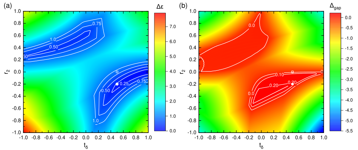
To examine the role of second-neighbor hoppings, we compute the flatness of the highest band defined by and the band gap defined by . Results are summarized in Figure S4. [Fig. 3 (a) in the main text is the combination of Figs. S4 (a) and (b).] In both plots, the location of with , the parameter set used in Fig. 2 (b) in the main text, is indicated by an open square, and the location of with , the parameter set used in Fig. 3 (b) in the main text, is indicated by a filled circle.
The Berry curvature of non-interacting electrons with and with is presented in Fig. S5.

2 model
Here, we show that a two-orbital model involving and orbitals, the model, has the same form as the model. In addition to and , we introduce , corresponding to in Ref. S 1. Using these three parameters, the hopping matrices are given by
| (S2) | |||
Defining , these matrices are simplified as
| (S3) | |||
A hopping matrix between site 1 and site 2 is schematically shown in Fig. S6. One notices that these matrices are identical to the hopping matrices for via with the change in sign in the off-diagonal elements.

Using the eigenstate of angular momentum for , the orbitals and are expressed as and , respectively. Using these relations, the SOC term, , in the subset is written as
| (S4) |
This form is also identical to the SOC in the model with a change in prefactor from to .
Supplementary Note 2 Many-body effects
This section discusses many-body effects in our kagome model.
1 Effective Hamiltonian
In multi-orbital systems, the local Coulomb interactions consist of several terms. This is simplified in a spin polarized state, where interaction terms contain the single spin component as . Here is the effective Coulomb interaction given by with the interorbital Coulomb repulsion and the interorbital exchange interaction . In general, there are other terms, such as the intraorbital Coulomb repulsion and the intraorbital pair transfer . All these parameters are needed to examine the relative stability between a spin polarized ferromagnetic states and others, such as antiferromagnetic states and a spin unpolarized state.
Now we focus on the highest-energy up-spin band, which has the Chern number . The kinetic term is given by , where is an annihilation (creation) operator of an electron on the highest-energy band at momentum and energy . and original electron operators are related by the unitary transformation as , where is the total number of unit cells and is the band index. We apply this unitary transformation to to obtain effective interactions in the highest band, i.e., . Since the full expression is rather lengthy, we provide only one example, local Coulomb interaction . This term becomes
| (S5) |
where in the function implies modulo and , with being two reciprocal lattice vectors. Using lattice translation vectors and , where the distance between nearest-neighbor sites is taken as the unit of length (see Fig. 1 in the main text), the reciprocal lattice vectors are given by and (See Fig. S7). The effective Hamiltonian is thus constructed as
| (S6) |
Here, involves and with appropriate phase factors.
2 Exact diagonalization
The effective Hamiltonian is diagonalized in momentum space. In this work, we consider a rhombus spanned by the two reciprocal lattice vectors and divide it into patches. This corresponds to having unit cells along the direction, so . Discretized momenta are now expressed as . We simply label discretized momenta using . Figure S7 depicts the momentum discretization used in this study with and
In this study, we consider a fractional filling . With , the number of electrons on the highest band is . In this case, the size of the Hilbert space is . Due to the translational symmetry and the momentum conservation of many-body interaction terms, is subdiagonalized according to the total momentum, modulo and . Using the same notation as the momentum discretization , each momentum sector has roughly states. The number of states of each momentum sector for our system is summarized in Table SI. Hamiltonian matrices can be diagonalized efficiently using, for example, ARPACK S 4.
| 0 | 1 | 2 | 3 | ||
|---|---|---|---|---|---|
| 0 | 30,709 | 30,624 | 30,704 | 30,624 | |
| 1 | 30,624 | 30,624 | 30,624 | 30,624 | |
| 2 | 30,709 | 30,624 | 30,704 | 30,624 | |
| 3 | 30,624 | 30,624 | 30,624 | 30,624 | |
| 4 | 30,709 | 30,624 | 30,704 | 30,624 | |
| 5 | 30,624 | 30,624 | 30,624 | 30,624 | |
3 Many-body Chern number
Many-body Chern number of the ground state is computed via S 3 where is the Berry curvature given by
| (S7) |
and is the many-body wave function constructed using single-particle wave functions after the Fourier transformation to momentum space. The momentum index will be omitted in the following discussion for simplicity.
Partial derivative of a wave function with respect to is approximated by the finite difference as . Here, the vector notation is used for , and or . Then, it is required to compute a product of two wave functions as with .
Since we are using a multiorbital model projected onto the flat band, a special care is needed. By diagonalizing a many-body Hamiltonian, the ground state in the momentum sector is given by
| (S8) |
where is the component of the unitary matrix, which diagonalizes the many-body Hamiltonian in the momentum sector , and means the ground state. form the basis set to describe the many-body Hilbert space. Specifically, this is given by
| (S9) |
Here, is a creation operator of an electron at the highest flat band at momentum , and is the vacuum. Note that matrices depend on the total momentum , but matrices do not because it is from diagonalising a single particle Hamiltonian. The product over is limited to a set of momenta specified by the index . The momentum shift and the twist phase are related via . Recalling that a creation operator is rewritten by creation operators of original electrons as , one finds
| (S10) |
Using this, is rewritten as
| (S11) | |||||
Considering small , because , is approximated to be . This leads to a simple expression
| (S12) |
This is used to compute products of two wave functions in Eq. (S7). For the integral over two boundary phases, we divide the boundary phase unit cell into meshes, numerically evaluate the partial derivative of the many-body wave function on each placket using a technique proposed in Ref. S 5, and sum up all the quantities.
References
- S (1) Slater, J. C. & Koster, G. F. Simplified LCAO Method for the Periodic Potential Problem. Phys. Rev. 94, 1498 (1954).
- S (2) Kang, M., Ye, L., Fang, S., You, J.-S., Levitan, A.,Han, M., Facio, J. I., Jozwiak, C., Bostwick, A., Rotenberg, E., Chan, M. K., McDonald, R. D., Graf, D., Kaznatcheev, K., Vescovo, E., Bell, D. C., Kaxiras, E., van den Brink, J., Richter, M., P.Ghimire, M., Checkelsky, J. G. & Comin, R. Dirac fermions and flat bands in the ideal kagome metal FeSn. Nat. Mater. 19,163 (2020).
- S (3) Niu, Q., Thouless, D. J. & Wu, Y.-S. Quantized Hall conductance as a topological invariant. Phys. Rev. B 31, 3372 (1985).
- S (4) Lehoucq, R. B., Sorensen,D. C., & Yang, C. ARPACK Users’ Guide (SIAM, Philadelphia, 1997).
- S (5) Fukui, T., Hatsugai, Y. & Suzuki, H. Chern Numbers in Discretized Brillouin Zone: Efficient Method of Computing (Spin) Hall Conductances. J. Phys. Soc. Jpn. 74, 1674 (2005).