Exploring the Connection between UV/Optical Variations and Radio Emission in Radio-Quiet Quasars: Clues on Radio Emission Origin2021Exploring the Connection between UV/Optical Variations and Radio Emission in Radio-Quiet Quasars: Clues on Radio Emission Origin–References

In order to build quasar sample with UV/optical variability measurements, we start from the SDSS Stripe 82 survey which covers about 290 $deg^{2}$ equatorial field of the sky and has been scanned over 60 times in the $ugriz$ bands by Sloan Digital Sky Survey (Sesar et al. 2007). MacLeod et al. 2012 provided the re-calibrated $\sim$10 years long light curves in $ugriz$ for 9258 spectroscopically confirmed quasars in SDSS Data Release 7 (SDSS DR7)¹¹ 1 http://faculty.washington.edu/ivezic/cmacleod/qso$\underline{~~}$dr7/Southern.html. 9120 out of them are located within the footprint of the Faint Images of the Radio Sky at Twenty-Centimeters (FIRST) survey, which is conducted with NRAO Very Large Array (VLA) in its B-configuration centered at 1.4 GHz and covers about 10,575 square degrees²² 2 http://sundog.stsci.edu (Becker et al. 1995; Helfand et al. 2015). The FIRST images have a resolution of $\sim$ 5^′′, and a typical rms sensitivity of 0.15 mJy. We cross-match with the FIRST catalog (Helfand et al. 2015) with a matching radius of 5$″$, and find 517 (5.7%) sources with FIRST counterparts. Among the FIRST detected sources, $\sim$ 80% could be classified as radio-loud based on their radio-loudnesses. This indicates while the dominant population of the sample is radio-quiet, some ($\sim$ 6%, assuming $\sim$ 10% of the 9120 quasars are radio-loud) radio non-detected sources could still be radio-loud.

We further match the quasars with Shen et al. 2011 to obtain their $z$, $M_{\rm BH}$, $L_{\rm bol}$ and $R_{\rm edd}$, where we adopt the fiducial virial $M_{\rm BH}$ from their catalog. 108 objects are further rejected due to the lack of $M_{\rm BH}$.

We adopt the same method as in Kang et al. 2018 to measure the intrinsic variability amplitude in each photometric band for each quasar. The variation amplitude is defined as excess variance $\sigma_{\rm rms}$ (Sesar et al. 2007; Zuo et al. 2012, e.g.,) as follows:

where $N$ is the number of photometric measurements for a single light curve, $X_{i}$ the magnitude for $i_{\rm th}$ observation, $\bar{X}$ the average magnitude, and $\sigma_{i}$ the $i_{\rm th}$ photometric uncertainty of each observation. We exclude $u$ and $z$ band data due to their significantly larger photometric uncertainties when compared with other three bands of $gri$. With only keeping the ones which have at least 20 epochs in each of the light curve to ensure accurate measurement of $\sigma_{\rm rms}$, our final sample consists of 8819, 8829, 8826 RQQs with UV/optical variability amplitude in $g$, $r$, $i$ band, respectively. Below we focus on $g$ band data as quasars are generally more variable in $g$ band than in $r$ or $i$ band. Unless otherwise stated, we present below the results using $g$ band $\sigma_{\rm rms}$, which are further verified by the well consistent results obtained using $r$ or $i$ band data.

In order to study the relation between radio emission and UV/optical variations in RQQs, we firstly divide our quasars equally into two subsamples according to $\sigma_{\rm rms}$, that is, a high-variability and low-variability subsample (hereafter HVQ0 and LVQ0 respectively).

However it is known that the UV/optical variability amplitude of quasars depends on physical parameters including luminosity, SMBH mass, Eddington ratio, and redshift (e.g. see Kang et al. 2018; Kang et al. 2021, and references therein). Indeed, according to Kolmogorov-Smirnov (K-S) test, the HVQ0 and LVQ0 subsamples we obtained above do have significantly different distributions in redshift, bolometric luminosity, SMBH mass and Eddington ratio, and LVQ0s have on average higher redshift, luminosity, SMBH mass and Eddington ratio (see Fig. 1). The radio flux in RQQs could also be sensitive to these parameters. A fair comparison to reveal the intrinsic connection between UV/optical variability and radio emission in RQQs should be made with these parameters matched.

As the stacked signals would be too weak if we split the samples into too many small bins in the multidimensional space of these parameters, we adopt two different approaches to divide the parent sample again into just two subsamples but with the parameters aforementioned matched between them. We first follow Kang et al. 2018 to perform multiple linear regression as follows:

We derive the residual $\sigma_{\rm rms}$ for each source from above equation, i.e., the difference between the observed $\sigma_{\rm rms}$ and the expected one based on the best-fit regression (see Fig. 2). And we divide the parent sample again into low-variability quasars (hereafter LVQ1) and high-variability quasars (HVQ1) based on the residual $\sigma_{\rm rms}$. The HVQ1 and LVQ1 subsamples do show consistent distributions of bolometric luminosity, SMBH mass and Eddington ratio (see Fig. 1), however the match in their redshift distributions is poor, likely because the dependence of $\sigma_{\rm rms}$ on redshift is more intricate than Equation 2 could describe³³ 3 Various lines which would shift into or out of SDSS $g$ band at certain redshifts could alter the values of $\sigma_{\rm rms}$ as the lines are less variable than the underlying continuum emission, leading to sharp dependence of $\sigma_{\rm rms}$ on redshift..

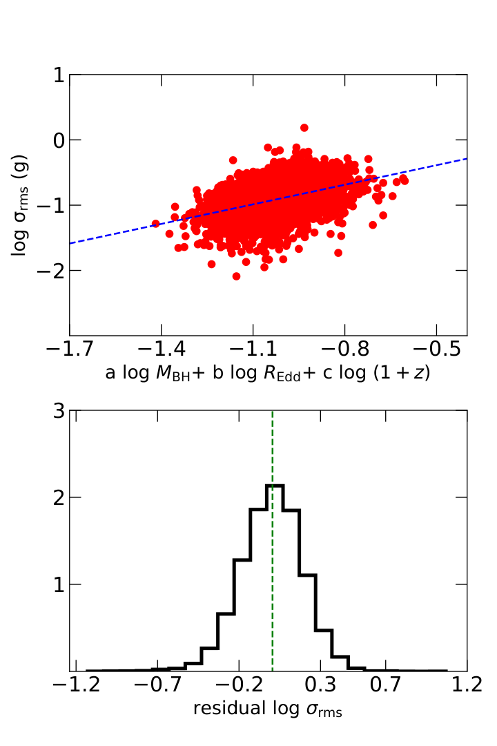
We then adopt a different approach to build HVQ and LVQ samples with better matched parameters. We randomly choose as many as possible and equal number of HVQ1s and LVQ1s (defined according to residual $\sigma_{\rm rms}$ in Fig. 2) in each three-dimensional bin of $z$, $M_{\rm BH}$, and $L_{\rm bol}$⁴⁴ 4 Here, using $R_{\rm edd}$ to replace $L_{\rm bol}$ would obtain same results. which contain both HVQ1s and LVQ1s. We endeavor to adjust the bins sizes of $z$, $M_{\rm BH}$, and $L_{\rm bol}$ to maximize the number of sources selected. Finally, we could select $\sim$ 88$\%$ sources out of the parent sample into HVQ2 and LVQ2 subsamples. This is because with the grid selection approach when unequal numbers of LVQ1s and HVQ1s fall in a grid, we have to drop sources to select equal number of LVQ1s and HVQ1s (Zhou & Gu 2021, e.g. see). As expected, the HVQ2 and LVQ2 subsamples derived with this approach show statistically consistent distributions in $z$, $M_{\rm BH}$, and $L_{\rm bol}$ and $R_{\rm edd}$ (see Fig. 1).

Below we describe the procedures we adopted to derive the stacked FIRST image of a sample of quasars. We extract from FIRST survey the radio cutout image for each quasar centred on the SDSS quasar position (with size of $30^{\prime\prime}\times 30^{\prime\prime}$, pixel size 1.8^′′). As most of our quasars are individually non-detected by FIRST, we employ the method of image stacking, a technique for combining data from many individual sources in order to study their statistical properties which are below the detection limit for a particular survey (White et al. 2007; Garn & Alexander 2009, e.g.,), to obtain the average radio emission. In this work, we adopt the median stacking approach, which is insensitive to outliers (i.e., the tails of the underlying flux distribution) and more robust for non-Gaussian distributions when compared with mean stacking (White et al. 2007). We align and median stack the individual FIRST images on a pixel-by-pixel basis (Radcliffe et al. 2021), using the python code of numpy.ma.median (van der Walt et al. 2011). The average radio flux density of a sample could then be derived from the stacked image. As a point-like source is centered at the nominal quasar(s’) position in each co-added image (see §3) and the changing PSFs from various individual FIRST images in the stacking are not CLEANed⁵⁵ 5 Although the most commonly used method to restore the flux density of a radio source from dirty image is CLEAN, maximum entropy and compressed sensing (Thompson et al. 2017), the flux density of a radio source can also be derived from the peak flux density in dirty beam when the source is very compact (i.e. point source). Since our RQQs are individually non-detected, their CLEANed images are not available. To avoid the problems caused by the fact that the PSF in the median stacked image is some kind of combination of various individual PSFs and it is not a CLEAN Gaussian, it is simpler to just use the value of central pixel as the peak flux density (Richard L. White, private communication)., following White et al. 2007, we use peak flux density only from the central pixel in each co-added image.

Another advantage of median stacking, when compared with mean stacking, is that the average radio flux derived from median stacking is less sensitive to the small population of radio-loud sources, and could better represent the dominant radio-quiet population. Note the FIRST images are not sufficiently deep to detect/exclude all radio-loud quasars from our sample. To further minimize the effect of the small population of FIRST non-detected but radio-loud sources, we derive the 45th percentile⁶⁶ 6 For each pixel in FIRST images to be stacked, we rank the flux densities in the pixel from all quasars in a sample, drop the 10% with largest flux densities, and derive the median for the rest 90%. instead of the simple median (50th percentile) while stacking FIRST images, to reduce the effect of the $\sim$ 10% radio-loud population. This is practically valid because some radio-loud sources, though non-detected, may have marginal/tentative signals in FIRST images, and thus the radio-loud fraction is expected to be even lower (or negligible) in sources with apparent FIRST pixel values in the bottom 45%. Note this approach (45th percentile) could only yield perfect measurement of average radio flux for RQQs (free from contamination by radio-loud ones) if the radio-loud fraction is 10% in the whole sample, and none of the sources with FIRST pixel values in the bottom 45% is radio-loud. Hereafter we refer the 45th percentile of the whole sample (including those FIRST detected) as the median of RQQs, if not otherwise specified.

We finally stress that directly adopting the median of the whole sample (instead of 45th percentile) would yield slightly higher average radio flux densities, however, it won’t alter the main results of this work. Using mean stacking wound not change the key results presented in this paper either.

Kang et al. 2018 investigated the relation between UV/optical variation amplitude ($\sigma_{\rm rms}$) and X-ray loudness ($L_{\rm X}/L_{\rm bol}$) using a sample of X-ray detected quasars in Stripe 82X (Ananna et al. 2017). They found that quasars with more intense X-ray radiation (controlling the effects of other physical parameters, i.e., $z$, $M_{\rm BH}$, $L_{\rm bol}$ and $R_{\rm edd}$) are more variable in the UV/optical. It can be interpreted that the UV/optical variations and X-ray emission are both associated with magnetic turbulence, i.e., the stronger disk turbulence, the more energy can be dissipated into the corona which could be heated through magnetic reconnection. We divide the sample of Kang et al. 2018 into high- and low-variability quasars as we built HVQ1 and LVQ1 in this work. We find that while the HVQ1 sample of Kang et al. 2018 is more variable than LVQ1 by a factor of 1.80 (which is similar to the difference between our LVQ1/HVQ1 and LVQ2/HVQ2), their HVQ1 are X-ray brighter on average by a factor of 1.5 than LVQ1.

The radio emission is expected to linearly correlate with X-ray according to the relation between X-ray and radio emission with $L_{\rm R}$ $=$ $10^{-5}$ $L_{\rm X}$ in RQQs reported in Laor & Behar 2008, probably driven by the Neupert effect (where $L_{\rm R}$ = d$L_{\rm X}/$d${t}$ as detected in stellar coronae, Neupert 1968; Guedel & Benz 1993). If so, we would expect our HVQ2 have radio emission $\sim$ 1.5 times stronger than LVQ2. However, our results show that the radio emission of HVQs are consistent with that of LVQs, contrary to the prediction (see the left panel in Fig. 7).

Our discovery thus indicates the 1.4 GHz FIRST radio emission of RQQs is unlikely driven by the central corona, or an extended region powered by the central corona. It would be intriguing to explore in the future the connection between UV/optical variability (thus X-ray loudness) and radio emission at higher frequencies, where the contribution of the corona to radio emission could be more significant.

On the other hand, if the radio emission in RQQs is dominated by weak jet, our discovery suggests that such jet should be driven by processes other than those which drive the the UV/optical variability and corona heating. Note Cai et al. 2019 suggested that the inner accretion disk of RLQs fluctuates less compared with RQ ones, likely because the stronger magnetic field in RLQs could stabilize the inner disc, i.e., implying a negative link between jet power and UV/optical variability. In this case, the tentatively negative relation between UV/optical variability and radio emission in RQQs reported in this work may support the scenario that the radio emission in RQQs is dominated by weak jet. Future studies of larger RQQ samples may reveal whether the tentatively negative relation is statistically robust, providing new clues to the radio emission origin.

The large-scale radio emission from star formation in the host galaxies may also fit our results (i.e., no statistically significant difference in radio emission between low- and high-variability quasars), as the accretion disk variations caused by random fluctuation may be no relevance with the host properties due to the origin of radio emission at spatial scales different by a factor of several orders. The scenario of star formation origin in RQQs is supported by recent low frequency radio observations. With Low Frequency Array (van Haarlem et al. 2013, LOFAR;) Two-metre Sky Survey (Shimwell et al. 2017, LoTSS DR1;), Gürkan et al. 2019 found that the 144 MHz continuum emission of RQQs (quasars with 0.1<$L_{144\rm{MHz}}$/$L_{i\rm{band}}$<100) is consistent with being dominated by star formation based on the far-IR to radio correlation measured in local star-forming galaxies (but note the far-IR to radio correlation may evolves with redshift). However, the weak jet contribution to 144 MHz radio emission in RQQs might also be non-negligible. Through modeling the LoTSS radio luminosity distribution of quasars assuming both jet and star formation contribute to radio emission in every quasar, Macfarlane et al. 2021 showed that the radio emission from jets is contributing down at least to the level comparable to the radio emission from star formation.

To summarize, we find more variable RQQs (at matched redshift, luminosity and SMBH mass) tend to have tentatively weaker radio emission, disfavoring the corona origin of radio radiation in RQQs. If the tentatively negative relation between UV/optical variability and radio emission in RQQs could be confirmed in the future, the weak jet origin would be preferred (or at least with significant contribution), as radio emission from star formation is expected to be irrelevant to the short term disc turbulence in quasars.

We have shown that RQQs with stronger UV/optical variability, which are known to have relatively stronger X-ray emission, do not show stronger radio emission. This poses clear challenge to the corona origin of the radio emission in RQQs. One might ask a simple question: why not directly explore the connection between X-ray and radio emission in RQQs?

First of all, the direct correlation between X-ray and radio power in RQQs may not yield useful constraints to the radio emission origin. Numerous previous statistical studies have revealed correlations between radio and X-ray emission in RQQs and RQ AGN (Brinkmann et al. 2000; Salvato et al. 2004; Panessa et al. 2007; Laor & Behar 2008; Panessa et al. 2015, e.g.,), seeming to support that their radio emission associates with the central engine of black hole activity instead of the star formation of host galaxies. This however does not necessarily support the corona origin of radio emission in radio-quiet AGN, because if the radio emission comes from jet, it is also expected to correlate with the bolometric power of AGN. Furthermore, studies also revealed correlations between the star formation rate and AGN power in radio-quiet AGN (Sargent et al. 2010; Thean et al. 2001; Macfarlane et al. 2021, e.g.), thus the correlation between radio emission and AGN power in radio-quiet sources does not necessarily imply an accretion related origin of the radio emission either.

What if we explore the relation between radio and X-ray emission in RQQs after controlling the effect of bolometric luminosity? Intuitively, this could be more straightforward than exploring the relation between UV/optical variability and radio emission. However, as we will show below, this approach is biased thus disfavored compared with the one adopted in this work.

For illustration, we explore the correlation between X-ray and radio emission in RQQs (controlling the effect of bolometric luminosity) with an X-ray detected SDSS quasar sample (without requiring variability measurement). We cross-match the fourth XMM-Newton serendipitous source catalogue (4XMM-DR9, Webb et al. 2020) with high SDSS DR7 quasar catalog of Shen et al. 2011 within 5^′′, resulting 4252 quasars with X-ray detection(s) where we only retain the one detection with the highest values of maximum-likelihood for those sources that have multiple detections. 4153 out of them fall in the coverage of FIRST survey, and they are further cross-matched with FIRST catalog within 5^′′ to exclude potential radio-loud quasars. We find and exclude 485 quasars with FIRST detections, i.e., a fraction of $\sim$ 11$\%$. We perform multiple linear regression to derive the dependence of X-ray (0.2$-$12 keV) luminosity on $z$, $M_{\rm BH}$, and $R_{\rm edd}$ (similar to Equation 2). We then divide the X-ray detected RQQs sample equally into X-ray brighter and X-ray-fainter subsamples, based on their residual X-ray luminosity with respect to the expected values derived from the best-fit regression. The K-S test results demonstrate that these two subsamples already have statistically indistinguishable distributions of $z$, $M_{\rm BH}$, $L_{\rm bol}$ and $R_{\rm edd}$. We find median peak flux densities 53.3${}_{-6.0}^{+5.6}$ $\mu$Jy and 48.5${}_{-4.3}^{+3.5}$ $\mu$Jy in X-ray brighter and X-ray-fainter subsamples⁷⁷ 7 Here, the peak flux densities is directly from the median (50th percentile) of the quasars after excluding the $\sim 11\%$ radio detected ones., respectively, also contrary to a linear correlation between X-ray and radio emission (see the right panel of Fig. 7).

But note that the X-ray brighter sample here yield slightly higher radio emission compared with the X-ray fainter sample, while our HVQ sample which is X-ray brighter than LVQ sample exhibits slightly lower radio emission than LVQ, although neither the differences is statistically significant. The subtle inconsistency between the two approaches could be due the uncertainties in bolometric luminosity or Eddington ratio. This is because the observed bolometric luminosity of an individual source could significantly deviate from the intrinsic value because of flux variability or inclination effect of the accretion disc emission, and since both radio and X-ray power correlates with the central engine, the uncertainties in bolometric luminosity could lead artificial partial correlations between radio and X-ray emission (Kang et al. 2018, e.g.). Though the results from two approaches are generally consistent, as the dependence of variability on bolometric luminosity is much weaker than that of X-ray or radio power (Kang et al. 2018, e.g., see Fig. 2 in), the primary approach presented in this work provides less biased results and thus is preferred.

References

- Ananna et al. (2017) Ananna T. T., et al., 2017, ApJ, 850, 66
- Baldi et al. (2021) Baldi R. D., Laor A., Behar E., Horesh A., Panessa F., McHardy I., Kimball A., 2021, arXiv e-prints, p. arXiv:2107.14490
- Becker et al. (1995) Becker R. H., White R. L., Helfand D. J., 1995, ApJ, 450, 559
- Behar et al. (2018) Behar E., Vogel S., Baldi R. D., Smith K. L., Mushotzky R. F., 2018, MNRAS, 478, 399
- Blandford & Königl (1979) Blandford R. D., Königl A., 1979, ApJ, 232, 34
- Blandford et al. (2019) Blandford R., Meier D., Readhead A., 2019, ARA&A, 57, 467
- Blundell & Beasley (1998) Blundell K. M., Beasley A. J., 1998, MNRAS, 299, 165
- Blundell & Rawlings (2001) Blundell K. M., Rawlings S., 2001, ApJ, 562, L5
- Blundell et al. (2003) Blundell K. M., Beasley A. J., Bicknell G. V., 2003, ApJ, 591, L103
- Bonzini et al. (2015) Bonzini M., et al., 2015, MNRAS, 453, 1079
- Brinkmann et al. (2000) Brinkmann W., Laurent-Muehleisen S. A., Voges W., Siebert J., Becker R. H., Brotherton M. S., White R. L., Gregg M. D., 2000, A&A, 356, 445
- Cai et al. (2016) Cai Z.-Y., Wang J.-X., Gu W.-M., Sun Y.-H., Wu M.-C., Huang X.-X., Chen X.-Y., 2016, ApJ, 826, 7
- Cai et al. (2018) Cai Z.-Y., Wang J.-X., Zhu F.-F., Sun M.-Y., Gu W.-M., Cao X.-W., Yuan F., 2018, ApJ, 855, 117
- Cai et al. (2019) Cai Z., Sun Y., Wang J., Zhu F., Gu W., Yuan F., 2019, Science China Physics, Mechanics, and Astronomy, 62, 69511
- Falcke & Biermann (1995) Falcke H., Biermann P. L., 1995, A&A, 293, 665
- Garn & Alexander (2009) Garn T., Alexander P., 2009, MNRAS, 394, 105
- Guedel & Benz (1993) Guedel M., Benz A. O., 1993, ApJ, 405, L63
- Gürkan et al. (2019) Gürkan G., et al., 2019, A&A, 622, A11
- Hardcastle & Croston (2020) Hardcastle M. J., Croston J. H., 2020, New Astron. Rev., 88, 101539
- Helfand et al. (2015) Helfand D. J., White R. L., Becker R. H., 2015, ApJ, 801, 26
- Hodge et al. (2011) Hodge J. A., Becker R. H., White R. L., Richards G. T., Zeimann G. R., 2011, AJ, 142, 3
- Hwang et al. (2018) Hwang H.-C., Zakamska N. L., Alexandroff R. M., Hamann F., Greene J. E., Perrotta S., Richards G. T., 2018, MNRAS, 477, 830
- Inoue & Doi (2018) Inoue Y., Doi A., 2018, ApJ, 869, 114
- Ivezić et al. (2002) Ivezić Ž., et al., 2002, AJ, 124, 2364
- Kang et al. (2018) Kang W.-y., Wang J.-X., Cai Z.-Y., Guo H.-X., Zhu F.-F., Cao X.-W., Gu W.-M., Yuan F., 2018, ApJ, 868, 58
- Kang et al. (2021) Kang W.-Y., Wang J.-X., Cai Z.-Y., Ren W.-K., 2021, ApJ, 911, 148
- Karim et al. (2011) Karim A., et al., 2011, ApJ, 730, 61
- Kellermann et al. (1989) Kellermann K. I., Sramek R., Schmidt M., Shaffer D. B., Green R., 1989, AJ, 98, 1195
- Kellermann et al. (1994) Kellermann K. I., Sramek R. A., Schmidt M., Green R. F., Shaffer D. B., 1994, AJ, 108, 1163
- Kellermann et al. (2016) Kellermann K. I., Condon J. J., Kimball A. E., Perley R. A., Ivezić Ž., 2016, ApJ, 831, 168
- Kelly et al. (2009) Kelly B. C., Bechtold J., Siemiginowska A., 2009, ApJ, 698, 895
- Kukula et al. (1998) Kukula M. J., Dunlop J. S., Hughes D. H., Rawlings S., 1998, MNRAS, 297, 366
- Laor & Behar (2008) Laor A., Behar E., 2008, MNRAS, 390, 847
- Leipski et al. (2006) Leipski C., Falcke H., Bennert N., Hüttemeister S., 2006, A&A, 455, 161
- MacLeod et al. (2012) MacLeod C. L., et al., 2012, ApJ, 753, 106
- Macfarlane et al. (2021) Macfarlane C., et al., 2021, MNRAS, 506, 5888
- Miller et al. (1993) Miller P., Rawlings S., Saunders R., 1993, MNRAS, 263, 425
- Mullaney et al. (2013) Mullaney J. R., Alexander D. M., Fine S., Goulding A. D., Harrison C. M., Hickox R. C., 2013, MNRAS, 433, 622
- Neupert (1968) Neupert W. M., 1968, ApJ, 153, L59
- Olsson et al. (2010) Olsson E., Aalto S., Thomasson M., Beswick R., 2010, A&A, 513, A11
- Padovani (2016) Padovani P., 2016, A&ARv, 24, 13
- Padovani (2017) Padovani P., 2017, Nature Astronomy, 1, 0194
- Padovani et al. (2017) Padovani P., et al., 2017, A&ARv, 25, 2
- Panessa & Giroletti (2013) Panessa F., Giroletti M., 2013, MNRAS, 432, 1138
- Panessa et al. (2007) Panessa F., Barcons X., Bassani L., Cappi M., Carrera F. J., Ho L. C., Pellegrini S., 2007, A&A, 467, 519
- Panessa et al. (2015) Panessa F., et al., 2015, MNRAS, 447, 1289
- Panessa et al. (2019) Panessa F., Baldi R. D., Laor A., Padovani P., Behar E., McHardy I., 2019, Nature Astronomy, 3, 387
- Radcliffe et al. (2021) Radcliffe J. F., Barthel P. D., Garrett M. A., Beswick R. J., Thomson A. P., Muxlow T. W. B., 2021, A&A, 649, L9
- Raginski & Laor (2016) Raginski I., Laor A., 2016, MNRAS, 459, 2082
- Salvato et al. (2004) Salvato M., Greiner J., Kuhlbrodt B., 2004, ApJ, 600, L31
- Sargent et al. (2010) Sargent M. T., et al., 2010, ApJS, 186, 341
- Sesar et al. (2007) Sesar B., et al., 2007, AJ, 134, 2236
- Shen et al. (2011) Shen Y., et al., 2011, ApJS, 194, 45
- Shimwell et al. (2017) Shimwell T. W., et al., 2017, A&A, 598, A104
- Smith et al. (2020) Smith K. L., et al., 2020, MNRAS, 492, 4216
- Thean et al. (2001) Thean A., Pedlar A., Kukula M. J., Baum S. A., O’Dea C. P., 2001, MNRAS, 325, 737
- Thompson et al. (2017) Thompson A. R., Moran J. M., Swenson George W. J., 2017, Interferometry and Synthesis in Radio Astronomy, 3rd Edition
- Ulvestad et al. (2005) Ulvestad J. S., Antonucci R. R. J., Barvainis R., 2005, ApJ, 621, 123
- Wang et al. (2021) Wang A., An T., Jaiswal S., Mohan P., Wang Y., Baan W. A., Zhang Y., Yang X., 2021, MNRAS, 504, 3823
- Webb et al. (2020) Webb N. A., et al., 2020, A&A, 641, A136
- White et al. (2007) White R. L., Helfand D. J., Becker R. H., Glikman E., de Vries W., 2007, ApJ, 654, 99
- White et al. (2017) White S. V., Jarvis M. J., Kalfountzou E., Hardcastle M. J., Verma A., Cao Orjales J. M., Stevens J., 2017, MNRAS, 468, 217
- Zakamska & Greene (2014) Zakamska N. L., Greene J. E., 2014, MNRAS, 442, 784
- Zakamska et al. (2016) Zakamska N. L., et al., 2016, MNRAS, 455, 4191
- Zhou & Gu (2021) Zhou M.-H., Gu M.-F., 2021, Research in Astronomy and Astrophysics, 21, 004
- Zuo et al. (2012) Zuo W., Wu X.-B., Liu Y.-Q., Jiao C.-L., 2012, ApJ, 758, 104
- van Haarlem et al. (2013) van Haarlem M. P., et al., 2013, A&A, 556, A2
- van der Walt et al. (2011) van der Walt S., Colbert S. C., Varoquaux G., 2011, Computing in Science and Engineering, 13, 22