Freeze-in Leptogenesis via Dark-Matter Oscillations
Abstract
We study the cosmology and phenomenology of freeze-in baryogenesis via dark-matter oscillations, taking the dark matter to couple to Standard Model leptons. We investigate viable models both with and without a symmetry under which all new fields are charged. Lepton flavor effects are important for leptogenesis in these models, and we identify scenarios in which the baryon asymmetry is parametrically distinct from and enhanced relative to leptogenesis from sterile neutrino oscillations. The models we study predict the existence of new, electroweak-charged fields, and can be tested by a combination of collider searches, structure-formation studies, X-ray observations, and terrestrial low-energy tests.
I Introduction
The nature of dark matter (DM) and the origin of the baryon asymmetry are two of the most important open questions in particle physics. In this paper we study an extension of the Standard Model (SM) that simultaneously addresses both questions. We consider a model of freeze-in DM McDonald 2002; Choi and Roszkowski 2005; Kusenko 2006; Petraki and Kusenko 2008; Hall et al. 2010; Bernal et al. 2017 involving two DM mass eigenstates, the mass splitting between which is sufficiently small that DM production, propagation, and annihilation are coherent processes in the early universe. In this situation, the different propagation phases associated with the two DM mass eigenstates can lead to SM particle/antiparticle asymmetries Shuve and Tucker-Smith 2020, along lines similar to asymmetry generation via oscillations of right-handed neutrinos in ARS leptogenesis Akhmedov et al. 1998; Asaka and Shaposhnikov 2005.
In the minimal version of the model we consider, the particles beyond the Standard Model (BSM) are a pair of gauge-singlet Majorana fermions (), which constitute the DM, and a complex scalar with charges under the SM gauge group. While is in equilibrium with the SM due to its gauge interactions, we assume that one or both of the are feebly interacting and never come fully into equilibrium. In two-component notation, the interaction term responsible for DM production is
| (1) |
where are left-handed spinors with hypercharge , representing the -singlet charged leptons of the SM, with flavor index . We work in the mass basis for both the DM and the SM leptons. Since carries only hypercharge, it can be as light as depending on its couplings to DM and SM fermions. This simple model is sufficient to obtain both the observed baryon and DM abundances.
As in the ARS mechanism, the production and oscillation of DM can generate asymmetries in individual flavors of SM leptons. Although the leading-order lepton flavor asymmetries sum to zero, flavor-dependent washout of these asymmetries can lead to a non-zero total lepton number asymmetry. However, our model also features potential sources for a flavor-summed asymmetry that are distinct from the ARS mechanism, arising from the asymmetry that can be stored in . In particular, the particle content allows to couple to the SM lepton doublets,
| (2) |
which can significantly impact both the asymmetry calculation and the collider phenomenology. This interaction violates the symmetry under which the BSM particles and are odd, leading to astrophysical signatures of DM decay such as X-ray lines.
Ref. Shuve and Tucker-Smith 2020 first established the mechanism of freeze-in baryogenesis via DM oscillations by studying a related model, in which the DM couples to a QCD-charged scalar and SM quarks. We briefly summarize the main findings of that paper. In the quark-coupled case, flavor mixing prevents the quarks from having flavor-dependent chemical potentials. This spoils the ARS mechanism, which depends critically on the presence of flavor-dependent asymmetries to generate a flavor-summed one. To find a non-zero asymmetry in the minimal realization, with a single QCD-charged scalar and two DM states, one needs to take into account the flavor-dependence of the quark thermal masses, particularly of the top quark. The DM must have a substantial coupling to the top quark for the asymmetry to be large enough, and the viable parameter space is tightly constrained, with the scalar having a mass of at most a few TeV. The parameter space broadens in the presence of an additional source of DM production, for example a second, heavier scalar whose decays leave behind a “primordial” coherent DM background. Even in this second scenario, the lightest scalar is typically not far above the TeV scale for parameters that work for both DM and baryogenesis. In either scenario, the DM mass is in the keV range, and the lifetime of the TeV-mass scalar typically satisfies cm, potentially leading to events with displaced jets plus missing transverse momentum at colliders. Finally, -violating terms for the quark-coupled case are tightly constrained by proton decay, making it more challenging for those interactions to be relevant for baryogenesis 11 1 More precisely, the -violating terms can be relevant in quark-coupled models only for certain matter content and coupling choices. Ref. Shuve and Tucker-Smith 2020 focused on the case in which the DM couples to the quarks of the SM, . With this choice, the relevant -violating term, is -violating (with the DM assigned ). If the DM instead couples to (and always defining to be an triplet), the -violating couplings and are -conserving but and are not. Finally, if the DM couples to , the only relevant -violating coupling is , which is -conserving..
As already mentioned, the mechanism of freeze-in leptogenesis has most commonly been discussed in the context of the production and oscillation of right-handed neutrinos in SM neutrino mass models Akhmedov et al. 1998; Asaka and Shaposhnikov 2005 (see Ref. Drewes et al. 2018 for a review). There has also been a recent proposal in which the freeze in of DM and baryogenesis are simultaneously achieved through the interference of tree and loop processes in the decay of a heavy mediator particle Goudelis et al., and there exist earlier proposals of asymmetric DM models in which SM and DM asymmetries are simultaneously generated through out-of-equilibrium scattering Hall et al.; Hook 2011; Unwin 2014.
I.1 Generation of flavor-dependent asymmetries

In this paper, we study three model benchmarks, each with a different mechanism that ultimately generates a baryon asymmetry. However, at leading-order in the DM couplings, the process that generates asymmetries in individual lepton flavors, depicted in Fig. 1, is always essentially the same.
Consider the DM interaction of Eq. (1), involving a single BSM scalar . For a generic DM coupling matrix , each decay produces a coherent superposition of DM mass eigenstates that depends on the flavor of the lepton produced in association. The DM abundance thus arises at . Subsequent DM oscillations and inverse decays generate flavor-dependent asymmetries at . SM-Yukawa interactions and sphalerons then produce asymmetries in other SM species as well. Neglecting neutrino masses, the three charges
| (3) |
are conserved in the SM, where is baryon number and is lepton flavor number. The final baryon asymmetry is proportional to , the charge stored in the SM sector, at the sphaleron decoupling temperature GeV D’Onofrio et al. 2014. In our bookkeeping, we always define the charges of the BSM particles to be zero, , even when we find it useful to regard one or both of these particles as carrying lepton number.
For sufficiently small , and assuming that the universe starts with after reheating, a perturbative calculation of the asymmetries is appropriate. The leading-order asymmetries turn out to be proportional to the coupling combination Akhmedov et al. 1998; Asaka and Shaposhnikov 2005
| (4) |
which means that the flavor-summed asymmetry vanishes at this order,
| (5) |
In the absence of additional model ingredients, then, no baryon asymmetry is generated at . We now define our three benchmark models, specifying how a final baryon asymmetry arises in each.
I.2 Model benchmarks
(1) The Minimal Model: Without the need for additional model ingredients, effects of and higher spoil the cancelation that leads to zero net charge at Akhmedov et al. 1998; Asaka and Shaposhnikov 2005. As in ARS leptogenesis, flavor-dependent washout can deplete the asymmetry in certain lepton flavors more than others, leading to an charge density that is equal to the asymmetry in DM. We take these effects into account at the perturbative level in Sec. II, and in Sec. III.1 we use the network of quantum kinetic equations (QKEs) presented in Appendix D.2 to solve for the cosmological evolution of the various flavor asymmetries and identify the viable parameter space for DM and leptogenesis.
(2) The UVDM Model: The cancelation of the baryon asymmetry at fourth-order in DM couplings assumes that the interaction of Eq. (1) is entirely responsible for DM production and annihilation. As for the case of DM couplings to QCD-charged states Shuve and Tucker-Smith 2020, an additional source of coherent production can strongly enhance the asymmetry Asaka et al. 2017; Shuve and Tucker-Smith 2020. There are many possibilities for this additional DM interaction; for concreteness, in Sec. III.2 we follow Ref. Shuve and Tucker-Smith 2020 by adopting a model with a second, heavier scalar , leading two coupling matrices, for and for . In this scenario the baryon asymmetry is proportional to
| (6) |
which does not vanish in general.
(3) The Z2V Model: Even if the interaction of Eq. (1) is the only coupling of the DM to the SM sector, additional interactions with SM fields can also qualitatively impact the asymmetry calculation, as we explore in Sec. IV. The -violating case admits two additional renormalizable interaction terms,
| (7) |
where is the SM Higgs doublet, are the SM lepton doublets, and we assume only a single scalar . X-ray line constraints on DM decay prevent the neutrino-portal couplings from playing a role in leptogenesis if is taken to be the DM Asaka et al. 2005; Asaka and Shaposhnikov 2005. By contrast, the Z2V couplings can be large enough to significantly modify the asymmetry calculation while being consistent with all experimental and observational constraints. These interactions violate , and they shift the charge densities produced by the DM interactions to produce a baryon asymmetry at . Moreover, we will see that the Z2V couplings can be large enough that the baryon asymmetry is dramatically enhanced relative to the Minimal Model. To be more precise, if all three independent Z2V couplings come into equilibrium, the lepton chemical potentials are driven to be flavor universal, which in turn drives all asymmetries to zero. If, however, only one or two of the Z2V couplings come into equilibrium, the baryon asymmetry is not washed out and effectively arises at .
I.3 Structure formation constraints
With the DM abundance generated at and the baryon asymmetry arising at or higher, a general challenge in these models is to produce a large enough baryon asymmetry without overproducing DM. Because we require the DM energy density to match the observed value, lighter DM means a larger DM number density and larger DM couplings, leading to a larger asymmetry. The DM/leptogenesis tension is therefore minimized by taking the DM to be as light as allowed by observational probes of structure formation. Constraints from Lyman- forest data are often expressed as a lower bound on , the mass of a warm thermal relic. Recent studies have obtained lower bounds on ranging from 1.9 keV Garzilli et al. 2019 to 5.3 keV Palanque-Delabrouille et al. 2020 at 95% confidence level; see also Refs. Baur et al. 2016; Baur et al. 2017; Iršič et al. 2017. A more stringent constraint on the dark matter mass applies in the type of freeze-in model we consider, with a heavy particle in thermal equilibrium decaying to out-of-equilibrium DM plus an additional light state. By matching matter power spectra, Refs. Kamada and Yanagi 2019; Ballesteros et al. 2021 find that the constraint keV translates to keV for freeze-in via two-body decay.
In the models we consider, with two DM mass eigenstates, it is possible possible for to be much lighter than this keV lower bound, provided that the DM energy density is dominated by . Moreover, this type of scenario is particularly advantageous for getting a large asymmetry, because can have larger couplings than would otherwise be allowed by the observed DM energy density. The authors of Refs. Boyarsky et al. 2009; Kamada et al. 2016; Baur et al. 2017 present constraints on mixed cold/warm dark matter in the plane, where is the fraction of DM energy density in the warm state. The most stringent constraints are obtained in Ref. Baur et al. 2017, which uses Lyman- forest data to find, at 2 CL, for , going down to for , at which point the bound on appears to have leveled off.
We take these findings into account in an approximate way. We require the mass of , the heavier DM particle, to satisfy keV. The lighter DM particle, , can be arbitrarily light provided that the fractional contribution to the DM energy density is sufficiently small. For Majorana-fermion DM that decouples at temperatures around or above the electroweak scale (as is the case in the models we consider), and which comes fully into equilibrium before decoupling, the observed DM energy density is realized for a DM particle mass of keV. For keV, then, is acceptably small regardless of the sizes of the couplings. We call keV the massless limit22 2 Even if it into equilibrium, a Majorana fermion of negligible mass that decouples at gives a contribution to well within the BBN and CMB constraints Brust et al. 2013..
We will study the massless limit to determine, for example, the full range of masses and lifetimes that work for DM and leptogenesis. We will will also identify viable parameter space with larger , under the assumption that points with give acceptable matter power spectra for arbitrary . A detailed and robust determination of the parameter space allowed by structure-formation constraints is work in progress, and beyond the scope of this paper. It is clear, however, that there exists abundant parameter space for DM and leptogenesis that does satisfy these constraints.
I.4 Outline of our analysis
The outline of the rest of the paper is as follows. In Sec. II, we present a perturbative analysis of DM and leptogenesis in the Minimal Model. The analysis provides useful context for understanding the results of subsequent sections while also motivating the need to work with the full system of QKEs to map out the viable parameter space more completely.
We present DM and leptogenesis results for the Minimal, UVDM, and Z2V models in Secs. III.1, III.2, and IV, respectively. For each model, we show results for the massless- limit to determine the range of allowed masses and lifetimes for the collider target (or lightest scalar, , in the UVDM model), along with the allowed range of DM masses. We also investigate what parts of the parameter space survive departure from the massless- limit: how heavy is allowed to be, and to what extent (if at all) must the couplings of the lighter DM state dominate over the couplings of ?
We find viable parameter space for all three models. In the Minimal Model, the upper bound on is TeV, and decays promptly in much of the viable parameter space. Moreover, the Minimal Model is constrained to be near its massless- limit: we need keV, and the couplings must be much larger than those of . In contrast, the UVDM Model has ample parameter space with keV and a long-lived particle. To a lesser degree, the Z2V Model also has viable parameter space with keV, with the scalar typically decaying promptly for scenarios in which the Z2V couplings significantly impact leptogenesis. Although larger masses are viable in the UVDM and Z2V Models, the largest asymmetries are realized for TeV. We discuss implications for collider searches and other experimental probes, including , in Sec. V.
We relegate certain technical details to a series of appendices. These include benchmark DM coupling matrices (Appendix A), equilibrium chemical potential relations (Appendix B), reaction density calculations (Appendix C), background for our adopted system of QKEs (Appendix D), and a discussion and collection of perturbative results (Appendix E).
II Perturbative analysis of the Minimal Model
II.1 DM versus flavor-dependent asymmetries
In this section, we quantitatively study the asymmetries alongside the DM abundance, all within the Minimal Model. In addition to highlighting certain qualitative aspects of asymmetry generation, this perturbative analysis also illustrates how the combined DM and leptogenesis requirements predict upper bounds on the masses of the new particles, making in particular a promising target for colliders. Our three model benchmarks share the same basic mechanism for the leading-order asymmetries, so this discussion is also a useful starting point for understanding our final DM and leptogenesis results. The reader more interested in those final results should skip ahead to Secs. III and IV.
This section draws from the perturbative results derived and collected in Appendix D.1 and Appendix E. For those results to apply, two conditions must be satisfied. First, the abundances of both mass eigenstates must remain well below their equilibrium values. Second, we need , where is the Hubble parameter at sphaleron decoupling and where
| (8) |
is the decay width in the Minimal Model, at leading order (e.g. neglecting thermal mass effects). This second condition ensures that washout processes, including those that do not depend on the DM abundance, have at most an order-one effect on 33 3 For , a asymmetry generated at has decayed by a factor by the time of sphaleron decoupling. We therefore adopt as our criterion for washout effects to be important, although this is of course based on a rough estimate.. The leading-order calculation of the DM abundance in Appendix E.1 leads to
| (9) |
where is the DM number-density divided by entropy density (defined to include both DM mass eigenstates but only one helicity state: or , not both), and is the equilibrium abundance for an individual helicity and mass eigenstate of particle. Eq. (9) shows that the perturbativity condition is the limiting one for larger masses.
The DM energy density, , is determined by , the DM masses and , and a mixing angle
| (10) |
which controls the DM composition produced by decays: at , the and number densities are proportional to and , respectively. In Appendix E.1 we find
| (11) |
where
| (12) |
is the average mass of the particles, weighted by abundance.
In Appendix E.1, we also show that the asymmetry (charge density divided by entropy density), evaluated at the sphaleron decoupling temperature , satisfies
| (13) |
where , is the observed baryon asymmetry Zyla et al. 2020, and the function is defined in Eq. (161) and plotted in Fig. 21(a). It is at most of order one, and depends on the oscillation parameter
| (14) |
where is the DM mass-squared splitting and GeV is defined so that the relation between Hubble parameter and the temperature is at early times. The inequality of Eq. (13) is saturated when the phases and additional mixing angles (besides ) that parametrize the DM coupling matrix take on appropriate values; see Eqs. (160) and (164) in Appendix E.
A typical state produced at high temperatures undergoes oscillations by the time the temperature drops to , at which point the abundance begins to become Boltzmann-suppressed. In Fig. 21(a), we see that , and therefore the asymmetry, is suppressed at large and small values of . For small , the oscillations do not have enough time to develop before the temperature becomes too small to have an appreciable rate for inverse decay. For large , the oscillations become rapid at early times, which cuts off the asymmetry growth prematurely. In Fig. 21(a), is peaked at for and for . The smallness of these optimal values reflects the importance of lower-energy particles (which oscillate more rapidly) and oscillations that occur at temperatures well below (whose effects are enhanced by the larger integrated time at lower temperatures).
We now take the massless- limit to see how large can be, consistent with the DM constraint. For fixed masses and fixed , the DM constraint allows us to determine and therefore . Taking and in Eq. (11), we find
| (15) |
which we can use to rewrite Eq. (13) as
| (16) |
Fig. 2 shows versus for various in the massless- limit. In this figure, the location of the peak shifts to higher as is increased. As the available time for oscillations is reduced (by increasing ), a shorter oscillation timescale (realized for larger ) is preferred.
If decays produce equal abundances of and (, i.e. maximal mixing), one can use Eq. (16) and the properties of the function to show that requiring leads to the upper bounds keV and TeV.
Eq. (16) shows a enhancement of for small mixing, . We can understand this enhancement as follows. In the massless- limit, the contribution to the energy density is negligible, and imposing the DM constraint amounts to choosing the couplings of , which are proportional to , in such a way that the energy density matches . That is, decreasing means increasing to keep the couplings held fixed. This causes an increase in the couplings, which are proportional , and therefore an increase in the asymmetry. Exploiting this effect allows to be realized for somewhat larger and masses than for the case of maximal mixing. However, the perturbativity condition provides a ceiling. One can use Eqs. (15) and (16) to show that the DM constraint, , and can only be simultaneously satisfied for keV and TeV.
Those are the largest masses that can give an asymmetry in an individual lepton flavor that is comparable to the observed baryon asymmetry, consistent with the DM constraint and roughly consistent with the perturbative assumption. A rather extreme optimization is required to realize these values, for example a particular texture for the matrix that that leads to decaying predominantly to a lighter DM mass eigenstate with keV. Moreover, we remind the reader that the flavor-summed asymmetry, and therefore the baryon asymmetry, is in fact zero at in the Minimal Model.
II.2 DM versus baryon asymmetry.
We now extend our perturbative study of the Minimal Model to , the order at which a baryon asymmetry arises. Throughout this section, we adopt an matrix of the form given in Eq. (57), with and the overall scale free to vary. The remaining parameters that define are fixed at values that are favorable for getting a large asymmetry (but not exactly optimal; see Appendix A.1 for details). For this choice of matrix, we find in Appendix E.1 that the final baryon asymmetry is
| (17) |
where the function is defined in Eq. (174) and plotted in Fig. 21(b). We get the maximum asymmetry, subject to the DM constraint, by taking the massless- limit. In that case we can use Eq. (15) to eliminate in Eq. (17), leading to the upper bound
| (18) |
for our benchmark matrix.
Keeping in mind that is never larger than , it is clear at this point that must couple preferentially to the lighter DM state, , for the asymmetry to be large enough. If decays instead produce equal and abundances (), the asymmetry of Eq. (18) is maximized for keV (which saturates our adopted structure-formation bound) and GeV. These additional optimizations only get the asymmetry up to .
To get a sense of the parameter space that opens up for smaller , we set , at the high end of what is reasonable for our perturbative analysis, and use Eq. (15) to eliminate in Eq. (18); the bounds we obtain in this way are guaranteed to apply only in the perturbative regime. We find that the DM constraint and can only be simultaneously satisfied for keV and GeV, with a maximum of about about six times the observed value for the optimal masses GeV and keV. For these optimal masses, Eq. (15) gives . So, our perturbative analysis suggests that the Minimal Model works for DM and leptogenesis within a rather constrained parameter space. In particular, must decay mostly to , which must be quite light – otherwise there would be nothing gained by having larger couplings than .
We now turn to a more detailed and comprehensive analysis of DM versus leptogenesis in the Minimal, UVDM, and Z2V Models.
III Results for -preserving scenarios
III.1 Results for the Minimal Model
To extend our study of the Minimal Model to larger values of , we turn to the system of quantum kinetic equations (QKEs) presented in Appendix D.2. In our implementation of the QKEs, which follows that of Refs. Hambye and Teresi 2017; Abada et al. 2019, the equations are integrated over momentum using a thermal ansatz for the DM momentum distribution; see Eq. (140). The QKEs track the and density matrices and the densities, all of which evolve slowly because only -induced interactions change them. The collision terms in the QKEs involve the and chemical potentials, which can be expressed in terms of the densities and the and density matrices using the asymmetry relations derived in Appendix B. For further details we refer the reader to the appendices.
To present results for the Minimal Model, we will first take the massless- limit to see the full range of masses and lifetimes and DM masses that work for DM and leptogenesis. Then we will see what happens to the viable parameter space as we increase . We will take essentially the same approach when we present results for the UVDM and Z2V Models.
For the benchmark matrix given in Eq. (57), and are determined once we specify , , and the BSM particle masses , , and . For Figs. 3 and 4, we take the massless- limit. Fig. 3 shows contours of in the mass-lifetime space for various , with chosen to satisfy the DM constraint at each point. The relation
| (19) |
is useful when connecting to our earlier perturbative analysis, in which we adopted as a rough cutoff on the perturbative regime, corresponding to cm. For the DM masses chosen for Figs. 3(a-d), we find that the QKE asymmetry is about a factor smaller than the perturbative one for GeV and . We will present a more detailed comparison of QKE and perturbative results for the UVDM and Z2V Models, in which a more significant proportion of the viable parameter space lives in the perturbative regime.
In Fig. 3(a), we take to be equal to 15 keV, our lower bound on the DM mass based on structure-formation considerations. The contour of this plot, which lies within TeV and cm, therefore represents our estimate of the full mass-lifetime parameter space for in the Minimal Model. The particle decays promptly (as far as collider searches are concerned) in much of the viable parameter space, and the relatively low ceiling on its mass makes a promising target for colliders. Baryon asymmetries over 100 times the observed value are in principle consistent with the DM constraint, but those large asymmetries require . Much of the viable parameter space has , consistent with expectations based on the perturbative analysis. In Figs. 3(b-d) we see the mass-lifetime space contract for larger , going up to 100 keV, which is roughly the largest viable DM mass in the Minimal Model.
To obtain these these results, we neglect thermal corrections to the DM masses. A proper treatment of these effects is quite involved due to the challenges of modeling the momentum modes that are important at . However, we have performed some numerical estimates of DM thermal mass effects that suggest that may be suppressed below the observed value in the small-, small- corners of the plots in Fig. 3. The impact is most significant for the keV plot, where our estimates indicate that lifetimes below cm for GeV, and below cm for GeV, may not be viable. The impacted lifetimes shift to lower values for larger , and we still find viable parameter space with as low as 100 GeV, without significant suppression in the the peak asymmetries realized at higher . Apart from the lower region just described, the viable parameter space is largely unaffected. We leave a more careful study of these effects for future work.
Still working in the massless- limit, Fig. 4 shows how the viable ranges of and expand as decreases. At fixed and , the asymmetry is suppressed as increases due to the smaller DM couplings required to match the observed DM energy density. At fixed and , the suppression of the asymmetry at large is due to the oscillations not having time to develop, while the suppression at small arises because significant dark matter production continues after asymmetry growth has slowed, requiring smaller DM couplings. Finally, at fixed , larger means a shorter oscillation timescale and a somewhat larger that maximizes the asymmetry. The more dramatic shift of the , keV contour to lower is a strong-washout effect. Washout suppression of the asymmetry depends on , while the DM energy density is proportional to for small . Once the DM constraint is imposed, is proportional to , leading to stronger washout at larger and lower .
Figs. 5 and 6 show the impact on the parameter space when we depart from the massless- limit, allowing a non-negligible fraction of the DM energy density to be stored in . In Fig. 5 we take GeV and keV, favorable for producing a large asymmetry, and show baryon asymmetry contours in the plane. We see that DM and leptogenesis require keV, even before we impose a constraint on , the fraction of dark matter energy density in . Once we impose , as favored by Lyman- forest observations, the constraint tightens to keV. Fig. 6 shows how the space shrinks as increases, with the effect becoming more pronounced for a more stringent upper bound on .
Our study of the Minimal Model shows that the viable parameter space is quite constrained, with the various upper bounds TeV, cm, keV, keV and 0.2. For much of the parameter space, the particle is a realistic discovery target for future runs of the LHC, as we discuss in Sec. V.1.
III.2 Results for the UVDM Model
The parameter space for DM and leptogenesis opens up significantly if we include an additional source of DM production Asaka et al. 2017; Shuve and Tucker-Smith 2020. For concreteness, we consider a model in which the DM couples to two scalars and , both of which have the same SM quantum numbers as the particle of the Minimal Model. We focus on the case with , so that impacts the dark matter and leptogenesis calculations only through the coherent background its decays leave behind. This “decoupled-” regime highlights the fact that the basic mechanism of asymmetry generation can work for any additional source of coherent DM production at high temperatures. Our study of the UVDM Model in this section has close similarities to the analysis of the scenario with two QCD-charged scalars in Ref. Shuve and Tucker-Smith 2020, although there are important differences as far as the associated collider phenomenology is concerned.
In the UVDM, two interaction terms are relevant for DM production,
| (20) |
The cancelation of the flavor-summed asymmetry at is spoiled in the presence of the two coupling matrices and . Furthermore, for both the asymmetry and DM calculations, the dependence on and is different than for and in the Minimal Model. This is largely because the DM abundance produced by decays is an additional free parameter, which we label as (defined to include both DM mass eigenstates but only one helicity state). We also now have two separate mixing angles describing the relative production of the two DM mass eigenstates: controls the branching ratios of to the lighter and heavier DM states, and does the same for . As before, small means that decays to are favored over decays to .
We present perturbative results for the UVDM Model in Appendix E.2. Eqs. (178) and Eqs. (180) give the DM energy density and baryon asymmetry, respectively. The asymmetry can be written as
| (21) |
where the function is defined in Eq. (181) and plotted in Fig. 21(c), and we define in the context of the UVDM Model. The factor depends on the phases and mixing angles that determine the two DM coupling matrices and ; see Appendix A.2 for details. We adopt an optimal benchmark for asymmetry generation with , as realized for the coupling matrices given in Eq. (64).
For selected DM masses and mixing angles, Figs. 7 and 8 show the viable mass-lifetime parameter space for . At each point on the mass-lifetime plane, the DM energy density produced by decays is determined, and the DM constraint is therefore satisfied by adjusting . In Fig. 7(a) for example, below and to the left of the diagonal line where the various contours become very narrowly separated, the DM energy density produced by exceeds , and the DM constraint cannot be satisfied.
The dashed contours in Fig. 7 are based on our perturbative results, Eq. (21) for and Eq. (178) for , while the solid contours in both Figs. 7 and 8 are obtained by numerically solving the QKEs introduced in Appendix D.2, with the initial condition taking into account the primordial abundance . Fig. 7 shows reasonable agreement between the perturbative and QKE calculations for cm; the differences at long lifetimes are mainly due to the thermal ansatz adopted for the DM energy distribution in the QKE approach.
For , the case of maximal mixing, and have equal overall coupling strengths and are produced with equal abundances. In this case, is long lived for most of the parameter space that works for DM and leptogenesis, with as large as tens of meters, as Figs. 7(a,b) show. Moreover, there is viable parameter space with comparable and masses, as we see in Fig. 7(b). This is all in sharp contrast to the Minimal Model, where we needed 1 keV, and cm for DM and leptogenesis to work. The UVDM parameter space extends out to larger masses than colliders will probe in the near future, but the largest asymmetries, over 100 times the observed value, are realized for 1 TeV.
Even larger is possible with small mixing (), but only in the massless limit. This is illustrated in Figs. 7(c) and (d). For keV, the suppression of from the small mixing angles is more than compensated by the larger overall size of DM couplings that match the observed DM energy density. Comparing Figs. 7(a) and (c), we see that small mixing allows for shorter lifetimes. Indeed, for small enough and , can be as small as in the Minimal Model. When the and masses are comparable, on the other hand, nothing compensates for the suppression of due to small and , and the viable parameter space shrinks dramatically, as seen in Fig. 7(d).
Fig. 8 shows how the mass-lifetime parameter space shifts and contracts as is increased. We take maximal mixing for Figs. 8(a-c), with , keV, and , respectively; the last of these three plots shows that in the UVDM Model, both DM masses can be well above those currently probed by Lyman- forest observations. Fig. 8(d) shows that even larger and masses are possible in a small-mixing scenario with . Here we restrict our attention to the massless- limit, because for these mixing angles and keV, the small viable parameter space shown in Fig. 7(d) quickly disappears as is increased.
Figs. 7 and 8 do not show the full extent of the UVDM mass-lifetime space one would find by maximizing the baryon asymmetry with respect to all other parameters. It turns out that masses of up to TeV can work for DM and leptogenesis, but only in the massless- limit, and with and all mixing angles and phases tuned appropriately. The required optimization is similar to what was presented in Appendix B of Ref. Shuve and Tucker-Smith 2020 for the case with QCD-charged BSM scalars. Our results here for the -coupled are consistent with the results of Ref. Shuve and Tucker-Smith 2020, once one takes into account the different spectator-effect factors and different gauge multiplicities.
In summary, broad ranges of parameters work for DM and leptogenesis in the UVDM Model, including scenarios with keV and comparably sized and couplings. Unlike in the Minimal Model, has a lifetime cm for much of the viable parameter space. We discuss the implications for LHC searches in Section V.1.
IV The Z2V Model
IV.1 Qualitative discussion
In this section we do not impose the symmetry that guarantees absolute DM stability in the Minimal and UVDM Models. There are now two interaction terms that can induce changes in the charge densities: the -preserving DM coupling and a new “Z2V” interaction term:
| (22) |
The Z2V term has the same gauge and flavor structure as an -parity-violating coupling often considered in supersymmetric theories; because the indices of the SM lepton doublets are contracted antisymmetrically, the is an antisymmetric matrix in lepton flavor, and there are therefore three independent Z2V couplings. We neglect a possible neutrino-portal coupling because, as we discuss in Sec. V.2.1, X-ray line constraints prevent them from being large enough to be relevant for leptogenesis. The couplings, on the other hand, can significantly impact the asymmetry calculation. The rough criterion for a Z2V coupling to come into equilibrium in the early universe is that the -induced decay width should be at least comparable to the Hubble parameter at , leading to
| (23) |
This is a far smaller coupling than has been probed experimentally. The X-ray line constraints on the couplings depend on the lepton flavors involved, but we will show in Sec. V.2.1 that they are rarely stronger than , and are often much weaker, for the parameter space that works for leptogenesis and DM. Other constraints on from low-energy experiments are never more stringent than , as we discuss in Sec. V.3.
To see how Z2V couplings might be relevant for leptogenesis, consider for simplicity a scenario with and (but not ) coupled to DM, and a single Z2V interaction involving and : At , there are no asymmetries in , , or the third-generation leptons, but we have equal and opposite asymmetries in and , and thanks to SM processes, equal and opposite asymmetries in and . Then the number of inverse decays will differ from the number of inverse decays, and a asymmetry is generated at . That is enough to guarantee a net charge in the SM sector at the same order. To see this, note that the interactions of Eq. (22) respect a generalized symmetry, with , , and 44 4 The DM Majorana masses do not respect this symmetry, but the associated effects come with suppressions and can be neglected.. No asymmetry arises at and, because the coupling does not involve DM, the asymmetry remains zero at . At this order, then, the SM sector has a charge equal in magnitude to that stored in .
Two simple observations turn out to have important implications for the viable Z2V Model parameter space. First, larger Z2V couplings can produce a larger asymmetry without increased DM production. Second, even if a coupling is large enough to invalidate the perturbative calculation of the asymmetry, that coupling does not necessarily lead to washout of the asymmetry. To illustrate the second point, we return to the simple example of the previous paragraph and consider the case in which is large enough that it comes fully into equilibrium. Imagine that equal and opposite number density asymmetries for and are first generated at (that is, ) and subsequently processed by , neglecting for simplicity spectator effects associated with SM processes. By conservation of the generalized , we have
| (24) |
where we set the asymmetry to zero because it arises only at higher order in . With in equilibrium we also have the chemical potential relation
| (25) |
We can solve this pair of equations for , taking , because is not involved in the Z2V coupling. This leads to a flavor-summed asymmetry
| (26) |
where we use the relativistic or non-relativistic relation between and depending on the temperature. We see that the flavor-summed asymmetry effectively arises at when comes into equilibrium. It makes sense that the asymmetry is Boltzmann suppressed at temperatures far below the mass. The charge in the SM sector is equal in magnitude to the sum of the charge stored in , which is zero at , and the charge stored in , which has essentially decayed away for . For sufficiently large , the dominant contribution to the asymmetry arises at . As explained in Appendix E.3.2, this contribution is distinct from the ARS one. It arises from the generation of a asymmetry at , followed by generation of an asymmetry due to decays to DM.
In our simple example with only and coupled to DM, the asymmetry would be driven to zero if the Z2V coupling that came into equilibrium were instead of . In that case, no asymmetry develops in the third-generation leptons, and Eq. (25) is replaced with , which when combined with Eq. (24) forces all chemical potentials to zero. More generally, for a generic matrix involving all active flavors, we should expect an asymmetry if one or two of the three Z2V couplings come into equilibrium. If all three Z2V couplings come into equilibrium, then the chemical potentials of all three leptons are forced to be flavor-independent, preventing any asymmetry from being generated at all55 5 This is true for the case of two DM mass eigenstates. For three or more DM mass eigenstates, an asymmetry can arise at even if all active flavors have the same chemical potential Abada et al. 2019; this is the case in a model considered in Ref. Shuve and Tucker-Smith 2020 involving a single QCD-charged scalar..
In our full calculation of the asymmetry, described in the following section, we take into account that the interactions continually process asymmetries as they are generated, and that SM spectator processes affect how the various asymmetries are related Shuve and Yavin 2014.
IV.2 Calculating in the Z2V Model
In the QKEs of Appendix D.2, the Z2V interactions do not enter into the evolution equations for the DM density matrices and . However, each Z2V interaction brings about a change in the charges, so the evolution equations for the associated charge densities do get modified. For example, if we have a single Z2V coupling , then each Z2V-induced decay, , produces the changes . As shown in Eq. (148), both and get contributions proportional to at leading order. The chemical potentials and can be expressed in terms of , , and using the results of Appendix B 66 6 The proportionality to holds if is satisfied. In our numerical work we allow for the possibility of highly asymmetric abundances using the approach described in Appendix D; see Eq. (150). This refinement is quantitatively unimportant in almost all scenarios we study in this paper, however..
Fig. 9 shows the effect on the baryon asymmetry when one or more Z2V couplings are large enough to come into equilibrium. For the chosen parameter point, and couple to DM, and a value well below the observed one arises in the absence of Z2V couplings. If a single Z2V coupling, , is large enough to come into equilibrium, , the final baryon asymmetry is enhanced by about two orders of magnitude relative to the -preserving case. If both and come into equilibrium, the final baryon asymmetry is again enhanced by a large factor, although only about half as large as for the case with a single Z2V coupling. Finally, if all three Z2V come into equilibrium, the asymmetry is strongly suppressed, as expected. For the parameters chosen, the asymmetry happens to change sign as is increased in this three- case, because the and contributions have opposite sign.
If one or two of the Z2V couplings come into equilibrium, the final baryon asymmetry is insensitive to the precise values of those couplings, as is evident in the plateaus at larger in Fig. 9. In this case, effectively arises at . To write down an expression for , it is convenient to define to be the “special” flavor singled out by the Z2V couplings: in the case of a single Z2V coupling in equilibrium, is the flavor whose lepton doublet is not involved in that -violating coupling, while in the case of two Z2V couplings in equilibrium, it is the flavor whose lepton doublet is involved in both of those couplings. In Appendix E.3 we show that is determined by , the asymmetry in the special flavor , calculated in the absence of Z2V couplings, i.e. using the Minimal Model result of Eq. (160). For example, if only comes into equilibrium, we have , and we get a baryon asymmetry at if and only if one would calculate an asymmetry in in the absence of the Z2V coupling.
More precisely, we find
| (27) | |||||
| (28) |
where the function is defined in Eqn. (79) and plotted in Fig. 20. The exponential suppression of at large leads to a Boltzmann-suppressed for , as we anticipated in the discussion surrounding Eq. (26). We evaluate at in Eqs. (27, 28) to get the final asymmetry. For our numerical studies in the rest of this section, we adopt the Z2V benchmark matrix of Eq. (68) and take one coupling in equilibrium, such that the asymmetry is maximized.
For Eq. (27) or (28) to be a good approximation for the baryon asymmetry, three conditions must be satisfied. First, one or two couplings must be large enough to come into equilibrium, while the remaining coupling(s) are small enough to remain well out of equilibrium, . Second, we need the couplings to be small enough to justify a perturbative treatment of the couplings, which means . Third, the contributions to the asymmetry must be subdominant, which is not the case if the asymmetry is strongly Boltzmann suppressed.
In the large- regime, is dominated by the contribution discussed earlier, given in Eq. (199) for our Z2V benchmark matrix. The asymmetry leads to an asymmetry that persists after the particles have disappeared, ensuring a surviving baryon asymmetry. The interplay between the and asymmetries will be evident in the results we present in the following section.
IV.3 Results for the Z2V Model
In Fig. 10 we see that the large enhancement of the asymmetry relative to the Minimal Model opens up a narrow region of viable parameter space with keV. In this plot, and are chosen to maximize the asymmetry subject to the DM constraint. One finds that is relatively large, , for the parameter space shown. We therefore expect that the perturbative result of Eq. (27), which is used in Fig. 10(a), should be more accurate than QKE results based on a thermal ansatz for the DM momentum distribution. The QKE calculation gives a smaller viable parameter space, but we see in Fig. 10(b) that the difference is mostly due to the thermal averaging. We show this by modifying the perturbative calculation to incorporate the same thermal ansatz, which amounts to using the function defined in Eq. (171) in place of in Eq. (160). The remaining discrepancy between the QKE and perturbative results is mostly due to the fact that our perturbative treatment approximates sphaleron decoupling to occur instantaneously at , whereas we take into account that sphaleron decoupling is a gradual process when we numerically solve the QKEs, following the approach of Ref. Eijima et al. 2017 (see Appendix D.2 for details).
For the relatively large values of shown in Fig. 10, the contribution to the asymmetry dominates throughout the viable parameter space. We consider the massless- limit in Fig. 11, which opens up the parameter space to smaller and larger . For Figs 11(a-c) we take keV and compare the QKE calculation with (a) the contribution, (b) the contribution, and (c) the sum of those two perturbative contributions. We see the Boltzmann suppression of the contribution for TeV, with the contribution dominating at larger . The same effect is evident in Figs. 11(d-f), for which we take keV. Here we see that increasing the DM mass shifts the parameter space for DM and leptogenesis to larger and smaller . In Figs. 11(c,f) the sum of the two perturbative contributions gives good agreement with the QKE result for sufficiently large .
For smaller , higher-order effects in become important and the perturbative treatment is not reliable. The relevant quantity for determining whether higher-order effects are important is , which is why the perturbative range for depends on . We get close agreement in the perturbative regime because we implement the same thermal ansatz for the DM momentum distribution in the perturbative calculation as in the QKE calculation. The poorer agreement at lower is mostly due to thermal mass effects, which are only significant in this region, and which are only included in the QKE calculation.
In Fig. 11, we include thermal averaging in our perturbative calculations as a consistency check with our QKE calculations. However, at least in the perturbative regime, not performing thermal averaging should yield a more accurate result. In Fig. 12, we include the full momentum dependence in the perturbative calculation. For keV, the and parameter space that works for DM and leptogenesis is limited to and 300 GeV 700 GeV, as we see in Fig. 12(a). Meanwhile, Figs. 12(b,c) should be compared with Figs. 11(c,f), which take the same DM masses but with thermal averaging. We see that the agreement with QKE results is not as close when we take thermal averaging out of the perturbative calculation. The discrepancy is again largest for GeV, where thermal mass effects are also significant, leading to QKE asymmetries more than five times smaller than the non-thermally-averaged perturbative ones. The QKE calculation nevertheless gives a reasonably accurate picture of the viable parameter space. Because the perturbative calculation becomes unreliable for sufficiently small , in the remainder of this section we use the QKE calculation to explore the full parameter space.


Fig. 13 shows the viable ranges of and masses in the Z2V Model for various , in the massless- limit. We see larger values compared with those in Fig. 4 for Minimal Model. Maximal mixing is viable for keV and 1 TeV, while for small , DM and leptogenesis can work for well beyond 10 TeV and well beyond 1 MeV.
For fixed , the peaks of the contours in Fig. 13 tend to shift to larger as the DM mass is increased. Larger DM mass means a shorter time scale for oscillations and asymmetry generation, which in turn means a larger optimal for generating an asymmetry subject to the DM constraint. This shift is obvious, for example, in the and plots, in which the DM couplings are big enough that contributions tend to give the largest asymmetries, but not so big to completely invalidate the perturbative approximation. The shift is less noticeable for the plots with large mixing, and . Here, the contribution is unimportant, and the Boltzmann suppression of the contribution prevents much movement to larger .
Because we take the massless- limit in Fig. 13, the DM couplings become larger for smaller and fixed . The contribution therefore increases in importance relative to the one as is reduced. For example, the features in the , keV contour reflect comparably sized, well separated peaks from the and contributions, whereas for and , the peak in the keV contour is heavily dominated by the contribution. For similar reasons, the keV peak shifts to larger for smaller , but the movement for keV is less pronounced because the contribution is itself peaked at lower , due to the longer oscillation timescale.
A power-law scaling of with is evident at large in Fig. 13. From Eqs. (199) and (198) one can show that for fixed , the asymmetry is proportional to in the regime in which only a small fraction of an oscillation has time to develop, . In Appendix E.3.2 we show that the maximum asymmetry, optimized with respect to and , falls off as for large , and that this delicate tuning of parameters can allow DM and leptogenesis to work out to TeV and MeV while staying at least roughly within the perturbative regime.
Finally, although many of the features of Fig. 13 can be understood at the perturbative level, the plot in particular is heavily impacted by effects higher-order in . For and keV, for example, we are in the strong-washout regime, and the interesting shape of the associated contour does not emerge at the perturbative level. Moreover, the contours in the plot clearly do not satisfy the perturbative relation for fixed and .
The impact on the parameter space due to structure formation constraints, which come into play for keV, can be seen in Figs. 14 and 15. For Fig. 14 we take the same and as for Fig. 5 for the Minimal Model, where we found we needed keV for DM and leptogenesis to work while satisfying . Applying the same constraint to the Z2V Model, we see that values two orders of magnitude larger the observed one are possible for keV, and that values up to several keV are viable. The appropriate bound on is dependent on the DM masses, the details of which we leave for future work. Fig. 15, which can be compared with Fig. 6 for the Minimal Model, shows how parameter space with larger opens up as the upper bound on is relaxed.
In this Section, we have seen that -violating interactions can qualitatively impact the parameter space for DM and leptogenesis. If one or two of the three independent couplings are large enough to come into equilibrium, the asymmetry is typically dramatically enhanced relative to the Minimal Model. This leads, for example, to viable parameter space with larger mixing angles and masses, keV. Finally, for a Z2V coupling to come into equilibrium, we need
| (29) |
For much of the Z2V-Model parameter space that works for DM and leptogenesis, far exceeds the minimum value for equilibration, and we have mm, in which case qualifies as promptly decaying as far as collider searches are concerned.
V Phenomenology
V.1 Collider constraints
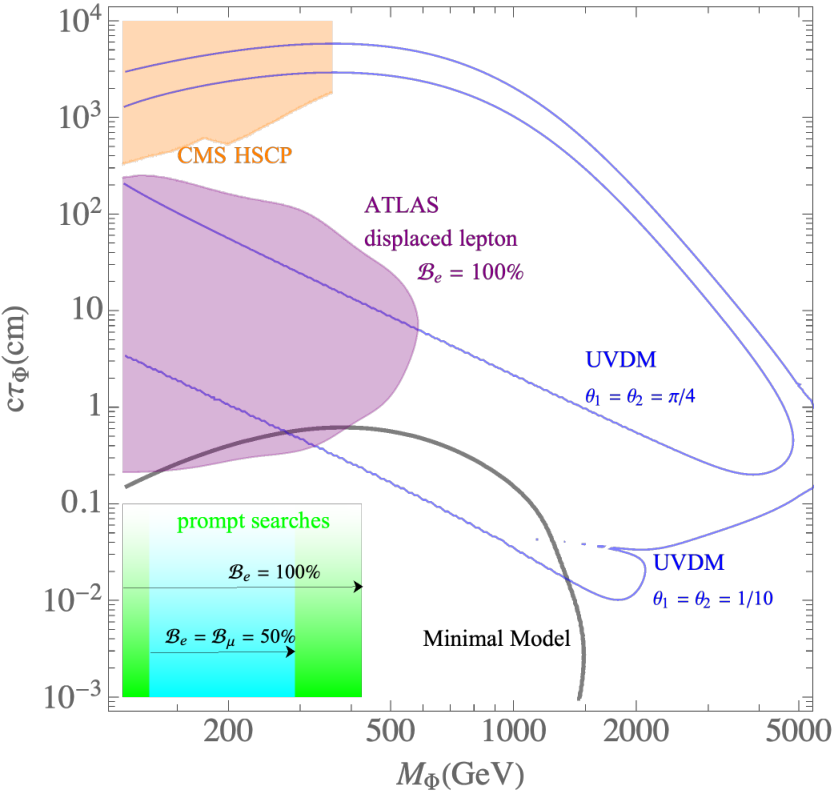
At the LHC, pair production would be followed by invisible, where the invisible particle is either a neutrino (in the Z2V Model) or DM (in the Minimal and UVDM models). In much of the viable parameter space for the Minimal and Z2V models, is short enough for CMS and ATLAS searches for promptly decaying sleptons to be effective Aad et al. 2020a; Sirunyan et al.; Sirunyan et al. 2019; Aad et al. 2014. In the UVDM Model, on the other hand, is typically long enough to bring searches for long-lived particles (LLPs) into play, including the ATLAS displaced lepton search Aad et al. and the CMS search for heavy stable charged particles (HSCPs) CMS 2016. Similar signatures have been proposed for other models of freeze-in DM Co et al. 2015 (for a recent study of LHC-friendly freeze-in models, see Ref. Bélanger et al. 2019).
Fig. 16 shows viable parameter space for the Minimal Model and, for selected parameters, the UVDM Model. For our Z2V Model benchmarks, with one or two Z2V couplings coming into equilibrium, much (but not all) of the parameter space has 1 mm, and the full mass range shown in Fig. 16 is viable; see Eq. (29) and Fig. 13. Fig. 16 also shows exclusion regions from LHC searches, with flavor-coupling assumptions and caveats specified below. The essential takeaway is that while LHC analyses have already probed some of the interesting parameter space for the each of the models, much of it remains open for exploration, particularly so if has an appreciable branching ratio to invisible.
While we have chosen models with an -singlet for detailed study, it is worth emphasizing that scenarios with an -doublet coupled to DM through an interaction term can work equally well for DM and leptogenesis. The collider phenomenology of a doublet can differ significantly from the singlet, especially in the presence of Z2V couplings, which can have arbitrary flavor structure provided that they are small enough to satisfy FCNC constraints. For example, a coupling can lead to decays of the neutral component of to opposite-sign, dileptons of any flavor combination. Alternatively, might decay hadronically via and/or couplings; if these hadronic decays are displaced and/or produce top quarks, they might result in a detectable signal. We set aside investigation of potential collider probes of the doublet case for future work, and now provide details on the various collider constraints on an -singlet .
V.1.1 Prompt searches
The collider constraints on a promptly decaying depend on its branching ratios , where for example . In the models we consider, it is appropriate to regard the DM as massless in the collider context. LHC searches Aad et al. 2020a; Sirunyan et al.; Sirunyan et al. 2019; Aad et al. 2014 then rule out and for and , respectively, while there is no LHC constraint for Aad et al. 2020b. At the top of the green shaded region in Fig. 16, which represents the exclusion for , the gradual fade-out around mm is meant to reflect our uncertainty regarding the degradation of prompt searches with increasing lifetime.
The leptogenesis mechanisms in the Minimal and Z2V models both require to couple to two or more lepton flavors. In fact, if Z2V couplings dominate decay, the largest branching ratio that any one flavor can have is ; specializing to the simple scenario in which a single Z2V coupling dominates, we have . Going beyond the single-flavor assumption in interpreting existing slepton search results is not completely straightforward. Consider, for example, a scenario with . Because of the same-flavor requirement, the signal efficiency for pair-production would be 1/2 that for a mass-degenerate pair in SUSY. Ref. Sirunyan et al. gives cross-section limits for combined and production. Bounding the NLO-NLL pair-production cross sections sus; Bozzi et al. 2007; Fuks et al. 2013; Fuks et al. 2014; Fiaschi and Klasen 2018; Beenakker et al. 1999 to be below twice those limits, we obtain the cyan exclusion region in Fig. 16: 77 7 Performing the same steps with the cross-section limits reported in Ref. Aad et al. 2020a does not appear to lead to any excluded region.. This exercise ignores that production would also lead, in the chosen scenario, to opposite-sign, different-flavor dilepton events, which are used to define control regions for background estimation in the analysis of Ref. Sirunyan et al.. For that reason, our exclusion region is tentative at best. We have also ignored that kinematic differences between and pair-production might lead to different efficiencies. However, the separate cross-section limits for LH and RH sleptons given in an earlier 13 TeV CMS analysis Sirunyan et al. 2019 are similar enough to suggest that this issue is unimportant.
The most recent ATLAS and CMS slepton search results do not include separate cross-section upper limits for selectrons and smuons. This complicates extracting limits when the or signals are suppressed by a significant branching ratio for invisible, even if we simply neglect the potential contribution to the signal from events with taus88 8 Light-flavor leptons produced from tau decays will differ kinematically from leptons directly produced by decay, and such decay modes have a total branching fraction of only 35%. We leave an estimate of the potential impact of invisible decays on searches in the , channels for future work.. For example, consider the two cases and . Ignoring events with s, the signal efficiency is now that for slepton pair-production. Taking into account the reported relative efficiencies for muons and electrons, the cross-section limits for combined and production given in Ref. Sirunyan et al. can be used to exclude narrow regions within the range for , while no region is excluded for . However, this exercise presumably underestimates the true sensitivity, because it includes background with both flavors of dilepton pairs even though the signal has a single flavor, electrons or muons. The 35.9 fb-1 CMS analysis Sirunyan et al. 2019 does give separate cross-section upper limits for smuons and selectrons, but they are not strong enough to constrain the and scenarios, assuming we can neglect decays to s.
These various observations motivate dedicated LHC analyses that target intermediate-mass “slepton-like” particles ( GeV) with lower values of than those associated with the multiple flavors of LH and RH sleptons of SUSY, including the possibility of mixed flavor in the final-state dileptons.
V.1.2 Displaced searches
For the longer lifetimes typical of the UVDM Model, the ATLAS displaced lepton search Aad et al. is relevant. The purple excluded region in Fig. 16 applies to the case with . The limits for are comparable; for example, the maximum mass excluded (for the optimal cm) lowers from GeV to GeV. For , there appears to be no excluded region for the optimal cm (although the mass range from 100–200 GeV is on the borderline).
The asymmetry generation mechanism in the UVDM model does not require to couple to multiple lepton flavors, but it is certainly allowed. We use the cross-section upper limits provided by Ref. Aad et al. to obtain rough estimates of the mass reach in such scenarios. For , and ignoring decays that do not involve electrons, the maximum excluded mass falls from GeV to GeV. For , and ignoring decays that do not involve muons, the maximum excluded mass falls from GeV to GeV.
V.1.3 Searches for heavy stable charged particles
Taking into account only direct stau pair production, a CMS search for HSCPs, Ref. CMS 2016, obtains a bound of approximately 360 GeV for a long-lived stau, for a SUSY parameter point in which the stau is mostly . This bound should apply to the model we consider for several meters. In Fig. 16 we roughly estimate the exclusion in the mass-lifetime plane by using the results of Ref. Junius et al. 2019 up to GeV and extrapolating those results up until GeV. The authors of Ref. Junius et al. 2019 find that when they apply their analysis to 8 TeV data, their results match reasonably well with the earlier study of Ref. Evans and Shelton 2016.
V.2 Astrophysical constraints
V.2.1 X-ray line constraints on the Z2V Model
In the presence of the -violating couplings of Eq. (7), the DM is unstable, and the partial width for decays is constrained by X-ray observations. The neutrino portal couplings induce -neutrino mixing, with mixing angle
| (30) |
The partial width for is Drewes et al. 2017; Shrock 1974; Petcov 1977; Lee and Shrock 1977; Marciano and Sanda 1977; Pal and Wolfenstein 1982; Shrock 1982; Barger et al. 1995 is
| (31) |
Results based on NuSTAR Perez et al. 2017; Neronov et al. 2016; Ng et al. 2019; Roach et al. 2020 and INTEGRAL Laha et al. 2020 data then constrain for DM masses ranging from 10 keV to 100 keV, corresponding to upper bounds on the overall neutrino-portal coupling strength of . These stringent limits justify neglecting the neutrino portal couplings in our asymmetry calculations.
We now focus on the Z2V couplings , which induce DM decays via diagrams such as that of Fig. 17, leading to a partial width of
| (32) |
where is the mass and are the masses of the SM leptons.
For purposes of illustration, we specialize to benchmarks with a single Z2V coupling in equilibrium and an matrix of the form described in Sec. A.3. These scenarios still allow a wide range of possible partial widths, depending on the SM lepton flavor running in the loop. For example, if the single Z2V coupling involves and () while the DM couples to and , we get
| (33) |
for the partial width of the heavier DM particle. Permuting the flavors involved in the and couplings leads to the same result except with replaced by or . For these benchmark scenarios, the partial width of is given by replacing in , but because might be too light to contribute to a detectable X-ray signal, we focus on .
The “-mediated” partial width of Eq. (33) leads to the X-ray bounds on shown in the left column of Fig. 18 (plots a, d, and g), for various in the massless- limit. At each point in the plane, is fixed by the DM density constraint. In regions that work for DM and leptogenesis, the upper bound on is typically and never below . The middle and right columns of Fig. 18 show the weaker bounds on that result when DM decays are instead mediated by muons or electrons, respectively, due to the flavor structure of the DM and Z2V couplings.
The couplings generate neutrino-portal couplings via the diagram of Fig. 17 with the photon line removed. To assess the potential impact of this radiative effect on DM decay, we consider the case in which the are negligible at the cutoff scale , leading to
| (34) |
at low energies, where is the SM Yukawa coupling for lepton flavor . We continue to focus on benchmarks with a single Z2V coupling, so that only one term contributes to the sum in Eq. (34), and only for one value of . The DM decay amplitude has a -suppressed “IR” contribution, which persists for , and a “UV” contribution proportional to , arising from radiative generation of the neutrino-portal couplings.
Although the IR and UV contributions should be combined at the amplitude level, for a simple comparison we evaluate the ratio
| (35) |
where is the partial width to in the limit, while is calculated using the neutrino portal couplings of Eq. (34) and otherwise neglecting the couplings (that is, ignoring 1/-suppressed contributions to the amplitude). The ratio depends on the flavor of SM lepton running in the loop. We show contours of and in Fig. 19, corresponding to -mediated and -mediated scenarios.
For GeV, the IR contribution dominates in either scenario, even for a Planck-scale cutoff. For 1 TeV, the UV contribution dominates for GeV in the -mediated scenario but is still subdominant in the -mediated scenario up to GeV. Unlike the upper bounds shown in Fig. 18, which are based on the IR contribution, the X-ray constraints on one derives taking into account only the UV contribution get stronger with increasing , due to the larger DM couplings required by the DM abundance constraint. However, the bound is never stronger than for the parameters shown in Fig. 18, even for GeV with in the loop.
V.2.2 Supernova constraints
Mixing of SM and sterile neutrinos is constrained by SN1987A. If the mixing angle is too large, an excessive fraction of the energy of the supernova explosion is carried away by the sterile neutrinos. One might expect the couplings of the particles in our models to be similarly constrained, but this is not the case in the Minimal and UVDM models. Even if the DM couples to electrons, the cross section for the process inside the core of the supernova is proportional to , versus the dependence for a weak interaction that produces a sterile neutrino. The constraints in the sterile neutrino case are never stronger than for any mass; see for example the “no-feedback” results of Ref. Suliga et al. 2020. Meanwhile, we typically need for DM and leptogenesis, so that is less than this upper bound by about fifteen orders of magnitude. In the Z2V model, can be produced singly with cross sections that are proportional to instead of . Here it is less obvious that the supernova cooling constraint can be ignored, although even a mild suppression from the factor seems likely to be enough to evade it. Moreover, these constraints become irrelevant if either the DM or Z2V couplings do not involve electrons, a scenario that works perfectly well for leptogenesis.
V.3 Other Z2V phenomenology
V.3.1 Constraints from low-energy probes
Various low-energy measurements constrain the parameter space of the Z2V Model. Some of the bounds can be inferred from earlier studies of superpotential terms in the context of -parity-violating supersymmetry, summarized in Ref. Barbier et al. 2005. To interpret these in the context of the Z2V Model, we replace the three flavors of right-handed sleptons by a single field and decouple the left-handed sleptons entirely.
Via tree-level exchange, a non-zero coupling affects the muon decay rate and therefore , which in turn affects the extraction of , , and from nuclear decays, kaon decays, and charmless meson decays. Refs. Barbier et al. 2005; Ledroit and Sajot 1998 obtain the constraint
| (36) |
The constraint does not change appreciably when we update the analysis using current PDG values for the CKM matrix elements Zyla et al. 2020. Measurements of atomic parity violation in cesium lead to a similar constraint on , while neutrino-electron scattering gives a weaker bound.
Exchange of can also lead to tree-level violation of lepton flavor universality. Focusing for simplicity on scenarios in which a single coupling dominates (neglecting possible cancelations), the current PDG average for the ratio leads to the constraints
| (37) |
| (38) |
The upper bound on is the same as reported in Refs. Barbier et al. 2005; Ledroit and Sajot 1998, while the upper bound on has strengthened following the BaBar measurement of Ref. Aubert et al. 2010. Similarly, updating the analysis based on the ratio of partial widths , we find
| (39) | |||||
| (40) |
The current bound on is significantly stronger than that obtained at the time of the original analysis Barbier et al. 2005; Ledroit and Sajot 1998, while the bound on has again not changed much.
If two or more couplings are sufficiently large, Z2V interactions can lead to lepton flavor violating signals. Updating the bound given in Ref. Barbier et al. 2005 to take into the current experimental limit (90% CL)Baldini et al. 2016, we obtain
| (41) |
as the constraint on the Z2V Model.
To obtain the bound from conversion we follow Ref. de Gouvea et al. 2001. The ratio of the conversion rate relative to the overall muon capture rate is
| (42) |
where we neglect any direct coupling of to quarks. The effective vertices are de Gouvea et al. 2001
| (43) | |||||
| (44) |
with the others zero. We therefore have
| (45) |
The strongest current limits are from the SINDRUM-II experiment, where gold () was used as the target nucleus. The muon capture rate for gold is Suzuki et al. 1987. The effective atomic number is Suzuki et al. 1987; Chiang et al. 1993. Finally, we need the nuclear form factor . Although Ref. Chiang et al. 1993 does not provide these form factors for gold, it does provide them for lead ():
| (46) | |||||
| (47) |
Ref. de Gouvea et al. 2001 appears to take a weighted average of the form factors according to the number of protons and neutrons. This gives us . Using the SINDRUM-II limit Bertl et al. 2006, we find the limit
| (48) |
This constraint is much stronger if there exist both LH and RH sleptons due to log enhancements of the Feynman parameter integrals, but since we only have a RH-type scalar the bound is much weaker.
For an analysis of decays, we again follow Ref. de Gouvea et al. 2001. In terms of the same loop-induced FCNC photon vertices of Eqs. (43,44), the branching fraction is
| (49) |
The current PDG limit, , then gives
| (50) |
a limit that is slightly stronger than than for conversion but less stringent than .
V.3.2 The anomaly
Measurements of the muon anomalous magnetic moment, , by the BNL E821 and Fermilab Muon experiments may indicate the need for new physics beyond the SM Bennett et al. 2006; Abi et al. 2021. Ref. Abi et al. 2021 puts the discrepancy between experiment and SM theory at
| (51) |
using the combined BNL and Fermilab measurements and the SM value determined by the Muon Theory Initiative Aoyama et al. 2020.
In the Z2V Model of Sec. IV, receives a negative contribution from a one-loop diagram with and SM leptons running in the loop. We can extract the contribution from the results of Ref. Kim et al. 2001, which considered in the context of -parity-violating supersymmetry. One finds Kim et al. 2001
| (52) |
In the model we have focused on in this paper, with an electroweak-singlet , it is therefore not possible to explain the discrepancy.
On the other hand, a explanation may be possible in the model variation with an electroweak-doublet for special arrangements of parameters. Consider for concreteness a scenario in which DM couples only to the SM lepton doublets of the first two generations, while has a single Z2V coupling, to :
| (53) |
Taking to be large enough to come into equilibrium in the early universe, a baryon asymmetry is generated at via the mechanism discussed in Sec. IV. The one-loop contribution to is Kim et al. 2001
| (54) | |||||
| (55) |
where is the mass of the electrically neutral particle. The discrepancy can thus be resolved for and GeV.
The special flavor structure assumed in Eq. (53) evades certain experimental constraints. In the absence of additional sources of lepton flavor violation (e.g. neutrino masses), the operators , , and are not generated radiatively. This can be seen from a symmetry under equal phase rotations of the fields , , , and , which is respected by the interactions of Eq. (53) and the SM charged-lepton Yukawa couplings. The interactions responsible for neutrino masses presumably violate this symmetry and cause these operators to be induced at some level, but these effects are model-dependent and generally come with additional loop and coupling suppressions99 9 Radiative contributions to an mass-squared term, which induces Higgs- mixing, come with similar suppressions. As usual for a mass-squared term in the scalar potential, these radiative contributions are proportional to , where is the cutoff of the theory.. It is thus possible to satisfy the X-ray constraints considered in Sec. V.2.1, even for the small masses and large Z2V couplings required by the anomaly.
At the LHC, pair production would lead to events with pairs. A detailed study would be required to determine the status of this scenenario with respect to existing LHC searches. The CMS search for LFV Higgs decays Sirunyan et al. 2021, which constrains the branching ratio for to be below 0.15% at 95% CL, might be relevant, but there are various aspects of that analysis that would seem to seriously reduce the signal efficiency for pair production. These include a veto on extra leptons and boosted decision tree variables chosen based on the kinematics of events, which differ significantly from those of events with pair-production of particles that decay to .
VI Conclusions
The freeze-in production and oscillation of DM provides a simple and well-motivated mechanism for baryogenesis. When DM couples to SM leptons, there must exist at least one new electroweak-charged scalar that can be as light as 100 GeV, and its couplings to the SM affect both the magnitude of the resulting asymmetry as well as the phenomenology. We have identified three benchmark models of interest that highlight the novel cosmology and signatures: a minimal scenario in which there exists a single new scalar and all non-SM fields are charged under a symmetry that stabilizes DM; a scenario where primordial production of DM through an unspecified mechanism can provide an enhancement to the asymmetry; and, a scenario in which the symmetry is broken, and SM lepton flavor effects likewise enhance the asymmetry relative to the minimal model.
We have found the minimal model to be quite constrained, with the mass of the scalar, , required to lie below approximately 1.5 TeV such that high-energy collider searches could be sensitive to much of the parameter space favored by baryogenesis. In the other models, can be heavier, although in that case the couplings are typically aligned to couple preferentially to the lighter DM state, which has a mass well below 1 keV to give a subdominant contribution to the dark matter energy density. Current collider constraints arise from searches for prompt or displaced leptons and missing transverse momentum motivated largely by supersymmetry, but the different flavor structure in our models leads to a weakening of several of these constraints and motivates dedicated searches for scalars that can decay to multiple flavors of leptons.
Constraints from structure formation and dark radiation significantly impact the parameter spaces of all of the models, and so there are good prospects for observing a signal if the sensitivities can be improved. Furthermore, the model that violates the symmetry can give an observable X-ray line from DM decay and/or signals at low-energy terrestrial experiments, including a possible explanation of the anomaly for the case of an electroweak-doublet .
Acknowledgements.
We are grateful to Alex Kusenko, Jane Schlesinger, and Benny Weng for helpful conversations. The work of BS is supported by the U.S. National Science Foundation under Grant PHY-1820770 and by the Research Corporation for Science Advance through a Cottrell Scholar Award.Appendix A Benchmark matrices
A.1 Minimal Model
By appropriate phase transformations on the charged leptons, the matrix can be brought into the form
| (56) |
with and . The partial widths of to final states involving and are proportional to and , respectively. The DM energy density therefore only depends on , , , and , and not on any of the other angles or phases appearing in .
For our analysis of the Minimal Model, we adopt a benchmark in which only two lepton flavors couple. We take , , and , with and set to a common value, . With these choices, the asymmetry, which is given in Eq. (174), is proportional to . This factor is maximized for , and so we adopt
| (57) |
as our benchmark matrix for the Minimal Model. Having equal-strength couplings for the two active flavors, , gives zero asymmetry, because in that case the washout rate is the same for both flavors, and the ARS mechanism is spoiled.
For this benchmark, one finds that the combination of couplings appearing in the baryon asymmetry evaluates to
| (58) |
Performing a full numerical optimization for three active flavors, we find that this two-active-flavor benchmark gives an asymmetry that is and times the fully optimized symmetry for and for , respectively. So although our simple benchmark does not maximize the asymmetry (even at the perturbative level), it gives a reasonable estimate of the full viable parameter space for DM and leptogenesis.
A.2 Benchmark matrices for the UVDM Model
In the UVDM Model, the matrices and represent the couplings of DM to and , respectively. The leading-order baryon asymmetry is proportional to
| (59) |
where can be parametrized in terms of six mixing angles/phases Shuve and Tucker-Smith 2020,
| (60) |
with
| (61) | |||||
| (62) | |||||
| (63) |
and .
The baryon asymmetry is maximized for and , choices which define our UVDM benchmark. These parameters are realized, for example, for the coupling matrices
| (64) | |||||
| (65) |
in which only a single flavor of charged lepton couples.
A.3 Benchmark matrices for the Z2V Model
For the Z2V Model of Sec. IV, our benchmark matrix is motivated by scenarios in which either one or two of the Z2V couplings come into equilibrium. In both cases there is one “special” SM flavor: if a single Z2V coupling is in equilibrium, it is the flavor of SM lepton doublet that does not couple to ; if two Z2V couplings are in equilibrium, it is the SM flavor involved in both of those couplings. For this discussion, we label the special flavor with the index .
As we discuss in Appendix E.3,the baryon asymmetry turns out to be proportional to
| (66) |
We now refer back to the parametrization of the matrix in Eq. (56). For fixed values of and , the parameters relevant for the DM energy density, the maximum possible value of the quantity in Eq. (66) is
| (67) |
For example, for the maximum value is realized for , , and . That is, in scenarios with one or two Z2V couplings in equilibrium, having only two active flavors couple to DM turns out to be optimal for maximizing the asymmetry, in the perturbative regime.
We take our benchmark matrices to be ones in which and one additional flavor of RH lepton couple, and in which Eq. (67) is satisfied. For , one such matrix is
| (68) |
another would have zeros in the second row instead. For , the row of zeros can be the first or the third, and for it can be the first or second. These various flavor structures are equivalent as far as leptogenesis is concerned, although they have different collider implications.
Appendix B Chemical potential relations
B.1 General relations
Neglecting neutrino masses, SM interactions conserve the three charges , where is baryon number and the are charges associated with the three lepton flavors. We define the charges of the BSM particles and to be zero. The DM and Z2V interactions are both -violating, which allows non-zero densities to evolve starting from what we assume is a neutral state after inflation. In Appendix D, we write down a set of quantum kinetic equations (QKEs) that model the evolution of the and DM abundances, while in Appendix E we provide a perturbative calculation of these densities that are valid in the weak-washout limit.
To calculate a final baryon asymmetry, we need to take into account rapidly occurring SM spectator processes using the appropriate relations among the asymmetries of the various particle/antiparticle species. In this appendix we derive those relations. We include possible Z2V couplings from the start, which need not be in equilibrium, but do not include a neutrino-portal coupling for the DM. The -violating interactions are then
| (69) |
In the UVDM model, there exists an additional scalar field whose interactions can affect the chemical potential relations. However, in our work we restrict our discussion of the UVDM Model to the decoupled- regime such that is absent from the thermal bath at all cosmological times relevant for leptogenesis, and so its couplings are not relevant here.
Because the DM is light enough to be ultrarelativistic at sphaleron decoupling, we can neglect DM masses in this discussion. This allows us to treat the negative-helicity and positive-helicity DM states as a particle/antiparticle pair, and , carrying opposite values of conserved charges. We define the and charges of and to be , , and . With these definitions, the interactions of Eq. (69) conserve both and . We take to be conserved in general, with and separately conserved below the sphaleron decoupling temperature. The violation of induced by Majorana masses is inconsequential for the masses and timescales we consider.
For particle species , we define and , where is the number density and is the entropy density. The charge densities are , where are the charges of particle species . In this appendix we will see that we can express all asymmetries, including the baryon asymmetry , entirely in terms of the DM asymmetry and the three .
In terms of the and density matrices introduced in Appendix D, the DM asymmetry is . There are eleven additional particle/antiparticle asymmetries to consider, encoded in the chemical potentials , , , , , , and . We take the quark chemical potentials to be flavor-independent due to flavor non-conservation in the quark sector. Working in the electroweak symmetric phase and taking sphalerons to be fully in equilibrium, we have the following system of equations:
| (70) | |||||
| (71) | |||||
| (72) | |||||
| (73) | |||||
| (74) | |||||
| (75) | |||||
| (76) |
Eqs. (70-73) are enforced by SM Yukawa interactions and sphalerons being in equilibrium. Eq. (74) follows from hypercharge neutrality, with being the hypercharge of particle species , Eq. (75) similarly expresses neutrality under the conserved charge , and Eq. (76) simply reflects the definition of the charges, with the sum over restricted to SM particles. Eqs. (70-76) can be solved to express all asymmetries in terms of and , using the appropriate relations between number-density asymmetries and chemical potentials1010 10 Here we linearize in all chemical potentials including . In our numerical work we make the replacement to allow for the possibility of a highly asymmetric population at temperatures well below ; see also the discussion leading to Eq. (150).:
| (77) |
Here, is the entropy density and counts gauge and flavor degrees of freedom (e.g. , while for each flavor ). For simplicity, in Eq. 77 we neglect all masses (including thermal contributions) except for that of the particle, giving for SM fermions and for the SM Higgs doublet. We take into account the potentially large mass of the particle, which leads to a temperature-dependent expression for . Defining
| (78) |
we find
| (79) | |||||
| (80) |
Fig. 20 shows a plot of .
It is convenient to define to be the net charge stored in the SM sector:
| (81) |
Solving our system of equations then leads to
| (82) | |||||
| (83) | |||||
| (84) | |||||
| (85) |
In the QKEs, the washout terms depend on , , and . We use Eqs. (83-85) to substitute in for these quantities, leading to a closed system of equations for tracking and the .
Eqs. (82-85) apply for all scenarios we consider, in the electroweak symmetric phase and while sphalerons remain in equilibrium. For the perturbative calculations presented in Appendix E, we take these relations to hold until sphaleron decoupling, which we approximate as occurring instantaneously at GeV D’Onofrio et al. 2014; to calculate the final baryon asymmetry we evolve and from high temperatures to and then evaluate Eq. (82) at . When we numerically solve the QKEs of Appendix D.2, we take into account gradual sphaleron decoupling following the methods of Ref. Eijima et al. 2017, while continuing to use unbroken-phase relations. Electroweak symmetry breaking could be taken into account following Ref. Khlebnikov and Shaposhnikov 1996, but we expect these effects to be small. For example, for -preserving scenarios we find in the unbroken phase (see the discussion leading to Eq. (86) below), versus deep in the broken phase, a 7% difference.
B.2 Chemical potential relations in -preserving scenarios
In the Minimal and UVDM Models, we set the -violating couplings in Eq. (69) to zero. In this case we have an additional conserved with only and charged, oppositely. The and asymmetries are thus equal, and Eq. (85) then gives . These relations can also be understood as direct consequences of neutrality under , for two alternative BSM-particle lepton-number assignments, and , both of which are consistent with conservation in the -preserving case (neglecting masses, for the second assignment). With this simplification, Eqs. (82-85) become
| (86) | |||||
| (87) | |||||
| (88) | |||||
| (89) |
In these -preserving scenarios, the present-day baryon asymmetry is proportional to the asymmetry at sphaleron decoupling. For heavy particles, several TeV, the final baryon asymmetry thus suffers an exponential suppression if the lifetime is much shorter than the age of the universe at sphaleron decoupling, . In the Z2V Model, on the other hand, the and asymmetries need not be equal, and this exponential suppression is not guaranteed.
B.3 Chemical potential relations with one Z2V coupling in equilibrium
For the Z2V Model, we pay special attention to benchmarks in which one or two of the three independent couplings are in equilibrium, with the remaining coupling(s) small enough to neglect.
Consider the case in which exactly one Z2V coupling comes into equilibrium, and take the other Z2V couplings to be zero for simplicity. There is then one particular lepton flavor that is not involved in Z2V interactions. The chemical potentials of the two lepton flavors that do participate in Z2V interactions, which we label as and , satisfy the equilibrium relation
| (90) |
Using this relation along with Eqs. (82-85), which apply generally, we can express entirely in terms of and . We find
| (91) |
Although Eq. (91) applies whenever the coupling is in equilibrium, (where and ), we will only use it when treating the DM couplings perturbatively, and under the assumption that we can neglect Z2V couplings involving . In that context, and can be calculated without taking into account Z2V couplings and then plugged into Eq. (91) to get the baryon asymmetry. Provided a perturbative treatment of the DM couplings is appropriate, this is a good approximation even for non-zero and , as long as those couplings are small enough not to come into equilibrium. As discussed in Appendix E.3, effectively arises at either or when one Z2V coupling comes into equilibrium, while the contributions to from out-of-equilibrium Z2V couplings come with an additional suppression.
B.4 Chemical potential relations with two Z2V couplings in equilibrium
When two Z2V couplings come into equilibrium, we instead define as the lepton involved in both of the independent Z2V couplings, so that both and are in equilibrium, but is not. In this case it is convenient to use the equilibrium relations
| (92) |
and Eqs. (82-85) to express the baryon asymmetry as
| (93) |
The combination is unaffected by the in-equilibrium Z2V interactions. In the perturbative context, we can calculate that quantity and without taking into account the Z2V couplings and then plug those values into Eq. (93) to get the baryon asymmetry, provided the remaining coupling is small enough to remain out of equilibrium.
If all three Z2V couplings come into equilibrium, the lepton chemical potentials are flavor-universal, and one can use Eqs. (70-76) to show that all asymmetries are proportional to . In this paper we restrict our attention to models with two mass eigenstates, in which case it turns out all asymmetries vanish Abada et al. 2019.
Appendix C Reaction densities
In this appendix we provide expressions for reaction densities and related quantities that appear in the QKEs of Appendix D and in the perturbative results of Appendix E. Focusing first on interactions involving the DM, the momentum-integrated QKEs involve generalized reaction density matrices in space, , where labels the flavor of charge lepton involved, and indicates whether the associated effects survive in the absence of asymmetries (), are driven by a asymmetry ()1111 11 Note that and label different reaction densities for a single scalar, rather than reaction densities for different scalars., or are driven by an asymmetry (). These reaction densities have the form
| (94) |
where the phase space factor is
| (95) |
with , , and . Here, the and masses-squared, including the leading thermal contributions from the gauge coupling , are
| (96) | |||||
| (97) |
where we neglect contributions from the charged-lepton Yukawa couplings and from possible and interaction terms.
The integrands appearing in the reaction densities are
| (98) | |||||
| (99) | |||||
| (100) | |||||
| (101) | |||||
| (102) |
with
| (103) |
and where
| (104) |
are the standard Bose-Einstein () and Fermi-Dirac () distribution functions for vanishing chemical potential. Because we label by the sign appearing in the associated expression, and apply to particles that are odd and even under exchange, respectively.
Carrying out all integrations besides those over and , the reaction densities can be expressed as
| (105) |
with the implied replacement in , and with
| (106) |
In the Z2V Model, we also need to consider processes and their CP conjugates. The relevant reaction density (no longer a matrix in space), is
| (107) |
where and label the flavors of leptons involved, and where the overall factor of two arises from summation over gauge degrees of freedom. Here we use the notation
| (108) |
and
| (109) |
where in addition to the -related quantities defined before, we now have , , and
| (110) |
where is the gauge coupling. (In an attempt to avoid notational confusion below, we have used energy conservation to express in terms of and , the energy of of one of the two leptons.)
Carrying out the integration over and then the remaining angular integrations, the Z2V reaction density can be expressed as
| (111) |
where the limits of integration are now
| (112) |
The QKEs are challenging to solve numerically and we therefore use reaction densities averaged over momentum in these equations. In our perturbative calculation, however, we are able to determine the contributions of each momentum mode separately. For simplicity, we neglect thermal masses in all of our perturbative calculations. Reversing the order of integration in Eq. (105) and carrying out the integral gives
| (113) |
where
| (114) |
and where we continue to use the notation . The function will feature in the perturbative calculations of Appendix D.1 and Appendix E, in which we calculate asymmetries and the DM energy density at leading order in , while taking into account the full momentum dependence of the DM distribution function.
The perturbative calculations of Appendix E also involve the and reaction densities. Because we neglect thermal masses in our perturbative work, we can replace the integration in Eq. (105) with an integration over the same range, and we find that these two reactions densities can be expressed as
| (115) | |||||
| (116) |
with
| (117) | |||||
| (118) |
and
| (119) |
Appendix D Quantum kinetic equations
Consider a single comoving DM mode, characterized by a particular value of . For this mode, information about the and occupation numbers and quantum coherence in space can be encoded in a matrix, . Following Refs. Hambye and Teresi 2017; Abada et al. 2019, we take the quantum kinetic equation (QKE) for to have the form
| (120) |
In the absorption and emission terms, we neglect DM masses by taking , whereas in the commutator term we define to be diagonal matrix whose non-zero entries are . As discussed in Sec. III.1, we leave for future work the inclusion of thermal corrections to the DM masses, whose effects are most important for large DM couplings and small values of and . We have chosen to work in terms of flavor-specific rates for absorption and emission, with the lepton flavor involved in the interaction labeled by . In evaluating these rates we include only decay and inverse decay processes, , which leads to
| (121) |
| (122) |
where in general the and chemical potentials enter into the distribution functions and , and where we define the phase-space factor
| (123) |
As we did in Appendix C, we define and , with and defined in Eqs. (96-97). In Eq. (123), we can take to be any four-momentum satisfying and .
D.1 Perturbative treatment of the QKEs
We first analyze the QKEs with the goal of calculating the densities in the Minimal Model, at leading order. For this purpose, we can ignore chemical potentials in the distribution functions appearing in Eqs. (121-122). We will also neglect thermal masses.
We start by taking three steps to rewrite Eq. (120) in a more convenient form. First, we use the relation
| (124) |
which applies in the absence of chemical potentials. Here is the Fermi-Dirac function defined in Eq. (104), and we continue to use for the momentum of our comoving DM mode.
Second, we switch our independent variable from to
| (125) |
The entropy density and Hubble parameter can then be written as and , where is the effective number of relativistic degrees of freedom and GeV. We then have .
Third, we define interaction-picture quantities
| (126) |
where we take the time-evolution matrix to have the form
| (127) |
The relative phase acquired between the two mass eigenstates is
| (128) |
with .
Following these three steps, the QKE for our comoving mode can be written as
| (129) |
To get the equation for , we replace and .
The number density of particles, , is obtained by integrating over momentum and taking the trace. We define the matrix so that its trace is :
| (130) |
In a DM interaction involving lepton flavor , the changes in the charge and in the and populations are related by . We then have
| (131) |
where the subscripts on the right-hand side specify that only contributions associated with lepton flavor are to be included. Integrating both sides of Eq. (129) over momentum, we obtain
| (132) |
To evaluate at leading order, we plug Eq. (132) and the corresponding equation for into Eq. (131), using the expressions for and ; integrating Eq. (129) gives
| (133) |
while for we replace . After these steps, we get the following expression for the asymmetry:
| (134) |
Because we ignore chemical potentials in the emission rate, we can express in terms of the function introduced in Eq. (114):
| (135) |
We can verify this relation by carrying out the integrations in Eq. (121). Equivalently, we can start with the fact that, in the absence of chemical potentials, is related in a simple way to the reaction density defined in Eq. (94),
| (136) |
Using the expression for given in Eq. (113) again leads to Eq. (135).
In Eqn. (134), time evolution matrices appear through the interaction-picture matrices and . Defining the matrices
| (137) |
the trace involves
| (138) |
These steps lead to our final expression for the leading-order asymmetry,
| (139) |
which is used extensively in our perturbative analyses.
D.2 Momentum-integrated QKEs
To go beyond a perturbative treatment of the QKEs, we start by integrating Eq. (120) over momentum, assuming a thermal DM momentum distribution:
| (140) |
where . The commutator term can then be expressed in terms of the diagonal matrix
| (141) |
where . Linearizing in chemical potentials, we find
| (142) |
where and can be expressed in terms of the reaction densities introduced in Appendix C:
| (143) | |||||
| (144) |
The kinetic equations for are obtained via the substitutions , , , and :
| (145) |
with
| (146) | |||||
| (147) |
The densities change only due to DM interactions and Z2V interactions. Each DM interaction involving SM flavor produces equal changes to the charge density and the number-density asymmetry, . Each Z2V interaction that changes the number of () particles produces an opposite (equal) change in . Working from these facts, we find
| (148) |
where is defined in Eq. (107).
As written, the QKEs presented in this appendix are valid assuming it is appropriate to linearize the distribution functions in chemical potential:
| (149) |
Although is almost always satisfied in the scenarios of interest in this paper, we replace Eq. (149) with
| (150) |
in our numerical work, a recipe that effectively takes into account the possibility of a highly asymmetric background left behind at , while remaining valid in the regime.
We can express the chemical potentials appearing in the QKEs in terms of and , using the results of Appendix B. Then we numerically solve the system of QKEs to obtain for temperatures down to the . Having done that, we determine the final baryon asymmetry by following Ref. Eijima et al. 2017, which takes into account gradual sphaleron decoupling. That is, we take
| (151) |
where is calculated from using the relations of Appendix B, which assume sphalerons to be in equilibrium. We use the SM result for , because no new chiral states couple to sphalerons in our model.
Appendix E Perturbative results
E.1 Minimal Model
E.1.1 DM density in the Minimal Model
To calculate the DM abundance at leading order, we ignore inverse decays, neglect Pauli-blocking due to the abundance, and neglect thermal mass effects. Using the leading-order calculation of Appendix D.1, the number density divided by entropy density (which is equal to that for ) is
| (152) | |||||
| (153) |
where is given in Eq. (133). Here and for all of our perturbative results, we switch to a notation in which is number density divided by entropy density, a number rather than a matrix. We restrict the notation in which represents a matrix to Appendix D. We continue to use as our independent variable; see the paragraph containing Eq. (125).
Using Eqs. 153, 133, and 135, and taking to get the final abundance, we find
| (154) |
where we have defined the momentum-integrated quantity
| (155) |
with itself defined in Eq. (114).
The dark matter energy density, , is determined by , the DM masses and , and the parameter appearing in Eq. (56), which determines the relative abundances of and . We have
| (156) |
where
| (157) |
is the average DM mass for the particles produced in decays, and where the factor of two takes into account the two DM helicity states, and . Taking the observed DM energy density to be keV Zyla et al. 2020, we find
| (158) |
where is the Hubble parameter at sphaleron decoupling and
| (159) |
is the decay width.
E.1.2 asymmetry in the Minimal Model
In the Maxwell-Boltzmann approximation, the flavor asymmetry in can determined via a relatively simple and physically motivated calculation that separately considers decays, inverse decays, and DM oscillations in between. This is the approach introduced in Ref. Shuve and Tucker-Smith 2020. In the present work, we fully incorporate quantum statistics and find it more convenient to obtain the desired result via a perturbative analysis of the QKEs, which we perform in Appendix D.1, neglecting thermal mass effects. There we find that the asymmetry, as a function of , is
| (160) |
with
| (161) |
and
| (162) | |||||
| (163) |
Starting from the parametrization of Eq. (56), one can derive the bound (for any )
| (164) | |||||
| (165) |
Using this inequality and evaluating Eq. (160) at the sphaleron decoupling temperature, , we find
| (166) |
where
| (167) |
and where is the observed baryon asymmetry Zyla et al. 2020. We use Eq. (166) in the perturbative analysis of Sec. (II.1).
For , corresponding to , the asymptotic behavior of for large and small is
| (168) |
In Fig. 21(a) we see that peak values for range from for (at ) to for (at ).
The momentum-integrated QKEs of Appendix D.2 incorporate a thermal ansatz for the DM momentum distribution; see Eq (140). Adopting the same ansatz in the perturbative context amounts to modifying Eq. (161) by the replacements
| (169) |
and
| (170) |
where in the first replacement, is the average for a thermal distribution, while the second replacement involves the momentum-integrated function introduced in Eq. (155). After making these substitutions and carrying out the integration, Eq. (161) becomes
| (171) |
where “t.a.” specifies that a thermal ansatz has been adopted for the DM momentum distribution.
E.1.3 baryon asymmetry in the Minimal Model
In the Minimal Model, one can use Eq. (160) to show that the flavor-summed asymmetry vanishes at : . As discussed in Appendix (B.2), we have in the Minimal Model, so the and asymmetries vanish at as well.
A flavor-summed asymmetry arises at , via the standard ARS mechanism Akhmedov et al. 1998; Asaka and Shaposhnikov 2005. In the presence of an chemical potential for a particular flavor lepton (but with , and continuing to neglect the DM abundance), the difference between the rates per volume for and decays is , where the reaction density is given by Eq. (115) when thermal mass effects are neglected. Each decay produces a change , so at , the flavor-summed asymmetry at sphaleron decoupling is
| (172) |
Eq. (87), with , allows us to rewrite this as
| (173) |
Finally, from Eq. (86) we have , with . Using Eqs. (160) and (161), we can write the final baryon asymmetry as
| (174) |
with
| (175) |
For the numerical studies of Sec. III.1, we adopt the benchmark matrix introduced in Sec (A.1), so that Eq. (58) applies. For this benchmark we find
| (176) |
For , the asymptotic behavior of for large and small is
| (177) |
Fig. 21(b) shows versus for various .
E.2 Perturbative results in the UVDM Model
In the UVDM Model, we include a “primordial” population of particles produced at high temperatures. For concreteness, we adopt a model with two scalars and , which have hierarchical masses, , and independent DM coupling matrices and . At , the DM energy density can be expressed as
| (178) |
Here, and are the average masses for DM produced in and decays, respectively. Generalizing Eq. (157), we have
| (179) |
for ; and are determined from the coupling matrices and analogously to Eq. (56) for the Minimal Model. The first term in Eq. (178) gives the DM energy density due to decays, reproducing the result from Eq. (158) for the Minimal Model. The second term gives the DM energy density due to decays, which we express in terms of , the number-density divided by entropy density for DM particles from decays (defined to include both DM mass eigenstates but only one helicity state: or , not both), and the reference value , the equilibrium abundance for an individual helicity and mass eigenstate of particle. We express the contribution in terms of because we take to be decoupled as far as phenomenology is concerned. Its only impact is through the coherent background its decays leave behind.
In the UVDM Model, a baryon asymmetry arises at , due to production by decay followed by inverse decays to . We can obtain an expression for the leading-order baryon asymmetry by appropriate modification of the flavor-summed version of Eq. (160), which applies in the Minimal Model. We get
| (180) |
with
| (181) |
where we define in the context of the UVDM Model. Using the relations between and and and , the final baryon asymmetry can be reexpressed as
| (182) |
where , which is defined in Appendix A.2, satisfies . We take the bound to be saturated for our UVDM benchmark scenario, as it is for the matrices of Eq. (64) for example.
E.3 Perturbative results in the Z2V Model
We restrict our perturbative analysis of the Z2V Model to cases in which one or two of the three independent Z2V couplings come into equilibrium, and we neglect higher-order corrections induced by Z2V couplings that remain out of equilibrium. If all three Z2V couplings come into equilibrium the baryon asymmetry essentially vanishes, as discussed in Appendix B. In the Z2V Model, the DM abundance at is given by Eq. (154), as in the Minimal Model. However, because we assume that the Z2V couplings dominate the decay width, Eq. (158), which expresses the Minimal-Model connection between the dark matter abundance and the lifetime, no longer applies.
E.3.1 at in the Z2V Model
One Z2V coupling in equilibrium: Consider the case of a single Z2V coupling in equilibrium. Then, for the one lepton flavor that does not participate in -violating interactions, which we call , the result for is unaffected by the Z2V coupling, allowing one to use Eq. (160) for that flavor. Furthermore, at , there is no asymmetry, . This is the case in the Minimal Model, as discussed in Appendix B.2, and because the Z2V couplings do not involve , it remains true in the Z2V Model. Eq. (91) then allows us to write the baryon asymmetry in this scenario as
| (184) |
with calculated using Eq. (160). The final baryon asymmetry is given by evaluating all quantities at .
In fact, using , the equilibrium relation Eq. (90), and the general relations Eqs. (82-85), one can express all asymmetries entirely in terms of and , the two combinations of asymmetries that are not affected by the Z2V couplings and so can be calculated using Eq. (160). For example, we find
| (185) | |||||
| (186) | |||||
| (187) | |||||
| (188) |
which we use below.
Two Z2V couplings in equilibrium: Similarly, for the case with two Z2V couplings and in equilibrium, and neglecting the remaining coupling , Eq. (93) leads to
| (189) |
where we again use the result from the Minimal Model Eq. (160), to evaluate each of the three terms in the combination , which is not affected by Z2V couplings to the extent that we can neglect . We can express this combination entirely in terms of the Minimal-Model result for , using the fact that in the Minimal Model, giving
| (190) |
In this equation, is to be calculated using the Minimal-Model result, Eq. (160), even though that expression does not in fact give correct result for in the particular Z2V scenario under consideration.
Using , the equilibrium relation Eq. (92), and Eqs. (82-85), one can also express the other asymmetries in terms of , which we can again replace with twice the Minimal-Model result for . We find
| (191) | |||||
| (192) | |||||
| (193) |
We now take a moment to review the notation used in Eqs. (184–193). In Eqs. (184–188), which apply in the case of a single Z2V coupling in equilibrium, is the special flavor whose lepton doublet is not involved in that Z2V coupling. In Eqs. (190–193), which apply in the case of two Z2V couplings in equilibrium, is the special flavor whose lepton doublet is involved both of those Z2V couplings. Both sets of equations apply when both DM mass eigenstates and the remaining Z2V couplings remain well out of equilibrium: and for Eqs. (184–188) and for Eqs. (190–193). In both sets of equations, the Minimal-Model result, Eq. (160), is to be used to calculate the asymmetries appearing on the right-hand sides.
E.3.2 at in the Z2V Model
For large massses, , the overall factors of in Eqs. (184) and (190) exponentially suppress the baryon asymmetry (see Fig. 20). This is a consequence of the fact there is no asymmetry at this order, . The final baryon asymmetry is proportional to the charge in the SM sector at sphaleron decoupling. For , the abundance becomes Boltzmann suppressed before sphaleron decoupling, along with any asymmetry1212 12 In our perturbative analysis of the Z2V Model, we assume that at least one coupling comes into equilibrium, which guarantees that always holds. In -preserving scenarios, it is possible for a asymmetry to survive at temperatures . In the Z2V Model, decays via Z2V interactions prevent this from happening. . When the surviving at sphaleron decoupling is negligible, conservation of , expressed by Eq. (75), tells us that the surviving charge in the SM sector is determined by the asymmetry at .
A non-zero is generated by decays to DM in the presence of chemical potentials for and/or . For sufficiently large , then, the final baryon asymmetry effectively arises at .
The -induced contribution to is essentially the standard ARS one, equal to the right-hand side of Eq. (173). However, when considering this contribution in the Z2V Model there are two differences that arise relative to the Minimal Model.
First, the Z2V couplings complicate the dependence of the final baryon asymmetry on the DM couplings. To calculate the quantity in Eq. (173), one needs to express in terms of , using the temperature-dependent relations in Eqs. (185–187) or Eqs. (191–192). The final expression is a mess; in particular the coupling dependence cannot be summarized in terms of the usual ARS factor . For our Z2V benchmark matrix, given in Eq. (68), the -induced contribution to is not generally zero, even though the standard ARS coupling factor vanishes.
Second, and more importantly, in the Z2V case the baryon asymmetry does not necessarily disappear when the particles do, and consequently it possible to get a sufficiently large asymmetry for larger masses than in the Minimal Model. In the Minimal Model, the final baryon asymmetry is proportional to the asymmetry at sphaleron decoupling, and Eq. (174) is a good approximation for the final baryon asymmetry only to the extent that we can ignore washout of by decay, . In the Z2V Model, the baryon asymmetry survives even in the absence of a asymmetry at sphaleron decoupling, provided a asymmetry has been generated. For the Z2V perturbative result to be valid we only need the DM abundances to remain well below their equilibrium values, and in particular it is not necessary for to be satisfied. For large masses, , the perturbativity criterion based on the DM abundance is the less restrictive one.
The -induced contribution is special to the Z2V Model, because in the Minimal Model we have . In fact, the -induced contribution tends to dominate the -induced one in the Z2V case, due to the different combinations of distribution functions appearing in the and reaction densities. The new contribution to is given by the analogue to Eqn (172),
| (194) |
Using either Eq. (188) or Eq. (193) to express in terms of , which we evaluate using Eq. (160), we obtain
| (195) |
with
| (196) |
Here, the upper and lower signs apply to the cases of one and two Z2V couplings in equilibrium, respectively, is the function defined in Eq. (118), and takes into account the temperature-dependent conversion from to :
| (197) |
As before, the flavor appearing in Eq. (195) is the one that is either not involved in the Z2V coupling or the one that is involved in both Z2V couplings, for the cases of one or two Z2V couplings in equilibrium, respectively.
Taking a single Z2V coupling to be in equilibrium and , the asymptotic behavior of for large and small is
| (198) |
Fig. 21(d) shows versus for various .
For ,which is the case in which the contributions to the baryon asymmetry dominate, we can set when evaluating Eqs. (91) or Eqs. (93) at sphaleron decoupling to get the final baryon asymmetry, giving . Using this relation and specializing to the Z2V benchmark matrix defined in Eq. (68), we obtain
| (199) |
We have used Eq. (154) to express the asymmetry in terms of the number density of dark matter particles rather than the DM coupling strength. Eq. (199) applies for large masses, , and relies on a perturbative expansion that is valid for .
To get a sense of how large can be consistent with the DM and baryon asymmetry constraints, take and make the small angle approximation for . Imposing the DM constraint, one finds
| (200) |
For large masses, , the combination has a maximum of at . Aggressively taking , one finds that the observed baryon asymmetry can be achieved masses for masses up to TeV, requiring a mass of MeV and . For the more perturbative case , the observed baryon asymmetry can be achieved with masses up to TeV for MeV and .
References
- McDonald (2002) J. McDonald, Phys. Rev. Lett. 88, 091304 (2002), arXiv:hep-ph/0106249 [hep-ph] .
- Choi and Roszkowski (2005) K.-Y. Choi and L. Roszkowski, Proceedings on 11th International Symposium on Particles, Strings and Cosmology (PASCOS 2005): Gyeongju, Korea, 30 May - 4 June 2005, AIP Conf. Proc. 805, 30 (2005), arXiv:hep-ph/0511003 [hep-ph] .
- Kusenko (2006) A. Kusenko, Phys. Rev. Lett. 97, 241301 (2006), arXiv:hep-ph/0609081 [hep-ph] .
- Petraki and Kusenko (2008) K. Petraki and A. Kusenko, Phys. Rev. D77, 065014 (2008), arXiv:0711.4646 [hep-ph] .
- Hall et al. (2010) L. J. Hall, K. Jedamzik, J. March-Russell, and S. M. West, JHEP 03, 080 (2010), arXiv:0911.1120 [hep-ph] .
- Bernal et al. (2017) N. Bernal, M. Heikinheimo, T. Tenkanen, K. Tuominen, and V. Vaskonen, Int. J. Mod. Phys. A32, 1730023 (2017), arXiv:1706.07442 [hep-ph] .
- Shuve and Tucker-Smith (2020) B. Shuve and D. Tucker-Smith, Phys. Rev. D 101, 115023 (2020), arXiv:2004.00636 [hep-ph] .
- Akhmedov et al. (1998) E. K. Akhmedov, V. A. Rubakov, and A. Yu. Smirnov, Phys. Rev. Lett. 81, 1359 (1998), arXiv:hep-ph/9803255 [hep-ph] .
- Asaka and Shaposhnikov (2005) T. Asaka and M. Shaposhnikov, Phys. Lett. B620, 17 (2005), arXiv:hep-ph/0505013 [hep-ph] .
- Drewes et al. (2018) M. Drewes, B. Garbrecht, P. Hernandez, M. Kekic, J. Lopez-Pavon, J. Racker, N. Rius, J. Salvado, and D. Teresi, Int. J. Mod. Phys. A 33, 1842002 (2018), arXiv:1711.02862 [hep-ph] .
- (11) A. Goudelis, P. Papachristou, and V. C. Spanos, arXiv:2111.05740 [hep-ph] .
- (12) L. J. Hall, J. March-Russell, and S. M. West, arXiv:1010.0245 [hep-ph] .
- Hook (2011) A. Hook, Phys. Rev. D84, 055003 (2011), arXiv:1105.3728 [hep-ph] .
- Unwin (2014) J. Unwin, JHEP 10, 190 (2014), arXiv:1406.3027 [hep-ph] .
- D’Onofrio et al. (2014) M. D’Onofrio, K. Rummukainen, and A. Tranberg, Phys. Rev. Lett. 113, 141602 (2014), arXiv:1404.3565 [hep-ph] .
- Asaka et al. (2017) T. Asaka, S. Eijima, H. Ishida, K. Minogawa, and T. Yoshii, Phys. Rev. D96, 083010 (2017), arXiv:1704.02692 [hep-ph] .
- Asaka et al. (2005) T. Asaka, S. Blanchet, and M. Shaposhnikov, Phys. Lett. B 631, 151 (2005), arXiv:hep-ph/0503065 .
- Garzilli et al. (2019) A. Garzilli, O. Ruchayskiy, A. Magalich, and A. Boyarsky, “How warm is too warm? towards robust lyman- forest bounds on warm dark matter,” (2019), arXiv:1912.09397 [astro-ph.CO] .
- Palanque-Delabrouille et al. (2020) N. Palanque-Delabrouille, C. Yèche, N. Schöneberg, J. Lesgourgues, M. Walther, S. Chabanier, and E. Armengaud, Journal of Cosmology and Astroparticle Physics 2020, 038–038 (2020).
- Baur et al. (2016) J. Baur, N. Palanque-Delabrouille, C. Yèche, C. Magneville, and M. Viel, Journal of Cosmology and Astroparticle Physics 2016, 012–012 (2016).
- Baur et al. (2017) J. Baur, N. Palanque-Delabrouille, C. Yèche, A. Boyarsky, O. Ruchayskiy, E. Armengaud, and J. Lesgourgues, Journal of Cosmology and Astroparticle Physics 2017, 013–013 (2017).
- Iršič et al. (2017) V. Iršič, M. Viel, M. G. Haehnelt, J. S. Bolton, S. Cristiani, G. D. Becker, V. D’Odorico, G. Cupani, T.-S. Kim, T. A. Berg, and et al., Physical Review D 96 (2017), 10.1103/physrevd.96.023522.
- Kamada and Yanagi (2019) A. Kamada and K. Yanagi, Journal of Cosmology and Astroparticle Physics 2019, 029–029 (2019).
- Ballesteros et al. (2021) G. Ballesteros, M. A. Garcia, and M. Pierre, Journal of Cosmology and Astroparticle Physics 2021, 101 (2021).
- Boyarsky et al. (2009) A. Boyarsky, J. Lesgourgues, O. Ruchayskiy, and M. Viel, Journal of Cosmology and Astroparticle Physics 2009, 012–012 (2009).
- Kamada et al. (2016) A. Kamada, K. T. Inoue, and T. Takahashi, Physical Review D 94 (2016), 10.1103/physrevd.94.023522.
- Brust et al. (2013) C. Brust, D. E. Kaplan, and M. T. Walters, JHEP 12, 058 (2013), arXiv:1303.5379 [hep-ph] .
- Zyla et al. (2020) P. Zyla et al. (Particle Data Group), PTEP 2020, 083C01 (2020).
- Hambye and Teresi (2017) T. Hambye and D. Teresi, Phys. Rev. D96, 015031 (2017), arXiv:1705.00016 [hep-ph] .
- Abada et al. (2019) A. Abada, G. Arcadi, V. Domcke, M. Drewes, J. Klaric, and M. Lucente, JHEP 01, 164 (2019), arXiv:1810.12463 [hep-ph] .
- Shuve and Yavin (2014) B. Shuve and I. Yavin, Phys. Rev. D 89, 075014 (2014), arXiv:1401.2459 [hep-ph] .
- Eijima et al. (2017) S. Eijima, M. Shaposhnikov, and I. Timiryasov, JCAP 1711, 030 (2017), arXiv:1709.07834 [hep-ph] .
- Aad et al. (2020a) G. Aad et al. (ATLAS), Eur. Phys. J. C 80, 123 (2020a), arXiv:1908.08215 [hep-ex] .
- (34) A. M. Sirunyan et al. (CMS), arXiv:2012.08600 [hep-ex] .
- Sirunyan et al. (2019) A. M. Sirunyan et al. (CMS), Phys. Lett. B 790, 140 (2019), arXiv:1806.05264 [hep-ex] .
- Aad et al. (2014) G. Aad et al. (ATLAS), JHEP 05, 071 (2014), arXiv:1403.5294 [hep-ex] .
- (37) G. Aad et al. (ATLAS), arXiv:2011.07812 [hep-ex] .
- CMS (2016) Search for heavy stable charged particles with of 2016 data, Tech. Rep. (CERN, Geneva, 2016).
- Co et al. (2015) R. T. Co, F. D’Eramo, L. J. Hall, and D. Pappadopulo, JCAP 1512, 024 (2015), arXiv:1506.07532 [hep-ph] .
- Bélanger et al. (2019) G. Bélanger et al., JHEP 02, 186 (2019), arXiv:1811.05478 [hep-ph] .
- Junius et al. (2019) S. Junius, L. Lopez-Honorez, and A. Mariotti, Journal of High Energy Physics 2019 (2019), 10.1007/jhep07(2019)136.
- Aad et al. (2020b) G. Aad et al. (ATLAS), Phys. Rev. D 101, 032009 (2020b), arXiv:1911.06660 [hep-ex] .
- (43) https://twiki.cern.ch/twiki/bin/view/LHCPhysics/SUSYCrossSections13TeVslepslep, LHC SUSY Cross Section Working Group.
- Bozzi et al. (2007) G. Bozzi, B. Fuks, and M. Klasen, Nucl. Phys. B 777, 157 (2007), arXiv:hep-ph/0701202 .
- Fuks et al. (2013) B. Fuks, M. Klasen, D. R. Lamprea, and M. Rothering, Eur. Phys. J. C 73, 2480 (2013), arXiv:1304.0790 [hep-ph] .
- Fuks et al. (2014) B. Fuks, M. Klasen, D. R. Lamprea, and M. Rothering, JHEP 01, 168 (2014), arXiv:1310.2621 [hep-ph] .
- Fiaschi and Klasen (2018) J. Fiaschi and M. Klasen, JHEP 03, 094 (2018), arXiv:1801.10357 [hep-ph] .
- Beenakker et al. (1999) W. Beenakker, M. Klasen, M. Kramer, T. Plehn, M. Spira, and P. M. Zerwas, Phys. Rev. Lett. 83, 3780 (1999), [Erratum: Phys.Rev.Lett. 100, 029901 (2008)], arXiv:hep-ph/9906298 .
- Evans and Shelton (2016) J. A. Evans and J. Shelton, JHEP 04, 056 (2016), arXiv:1601.01326 [hep-ph] .
- Drewes et al. (2017) M. Drewes et al., JCAP 01, 025 (2017), arXiv:1602.04816 [hep-ph] .
- Shrock (1974) R. Shrock, Phys. Rev. D 9, 743 (1974).
- Petcov (1977) S. T. Petcov, Sov. J. Nucl. Phys. 25, 340 (1977), [Erratum: Sov.J.Nucl.Phys. 25, 698 (1977), Erratum: Yad.Fiz. 25, 1336 (1977)].
- Lee and Shrock (1977) B. W. Lee and R. E. Shrock, Phys. Rev. D 16, 1444 (1977).
- Marciano and Sanda (1977) W. J. Marciano and A. I. Sanda, Phys. Lett. B 67, 303 (1977).
- Pal and Wolfenstein (1982) P. B. Pal and L. Wolfenstein, Phys. Rev. D 25, 766 (1982).
- Shrock (1982) R. E. Shrock, Nucl. Phys. B 206, 359 (1982).
- Barger et al. (1995) V. D. Barger, R. J. N. Phillips, and S. Sarkar, Phys. Lett. B 352, 365 (1995), [Erratum: Phys.Lett.B 356, 617–617 (1995)], arXiv:hep-ph/9503295 .
- Perez et al. (2017) K. Perez, K. C. Y. Ng, J. F. Beacom, C. Hersh, S. Horiuchi, and R. Krivonos, Phys. Rev. D 95, 123002 (2017), arXiv:1609.00667 [astro-ph.HE] .
- Neronov et al. (2016) A. Neronov, D. Malyshev, and D. Eckert, Phys. Rev. D 94, 123504 (2016), arXiv:1607.07328 [astro-ph.HE] .
- Ng et al. (2019) K. C. Y. Ng, B. M. Roach, K. Perez, J. F. Beacom, S. Horiuchi, R. Krivonos, and D. R. Wik, Phys. Rev. D 99, 083005 (2019), arXiv:1901.01262 [astro-ph.HE] .
- Roach et al. (2020) B. M. Roach, K. C. Y. Ng, K. Perez, J. F. Beacom, S. Horiuchi, R. Krivonos, and D. R. Wik, Phys. Rev. D 101, 103011 (2020), arXiv:1908.09037 [astro-ph.HE] .
- Laha et al. (2020) R. Laha, J. B. Muñoz, and T. R. Slatyer, Phys. Rev. D 101, 123514 (2020), arXiv:2004.00627 [astro-ph.CO] .
- Suliga et al. (2020) A. M. Suliga, I. Tamborra, and M.-R. Wu, JCAP 08, 018 (2020), arXiv:2004.11389 [astro-ph.HE] .
- Barbier et al. (2005) R. Barbier et al., Phys. Rept. 420, 1 (2005), arXiv:hep-ph/0406039 .
- Ledroit and Sajot (1998) F. Ledroit and G. Sajot, “Indirect limits on SUSY Rp violating couplings lambda and lambda’,” (1998), http://hal.in2p3.fr/in2p3-00362621.
- Aubert et al. (2010) B. Aubert, Y. Karyotakis, J. P. Lees, V. Poireau, E. Prencipe, X. Prudent, V. Tisserand, J. Garra Tico, E. Grauges, M. Martinelli, and et al., Physical Review Letters 105 (2010), 10.1103/physrevlett.105.051602.
- Baldini et al. (2016) A. M. Baldini et al. (MEG), Eur. Phys. J. C 76, 434 (2016), arXiv:1605.05081 [hep-ex] .
- de Gouvea et al. (2001) A. de Gouvea, S. Lola, and K. Tobe, Phys. Rev. D 63, 035004 (2001), arXiv:hep-ph/0008085 .
- Suzuki et al. (1987) T. Suzuki, D. F. Measday, and J. P. Roalsvig, Phys. Rev. C 35, 2212 (1987).
- Chiang et al. (1993) H. C. Chiang, E. Oset, T. S. Kosmas, A. Faessler, and J. D. Vergados, Nucl. Phys. A 559, 526 (1993).
- Bertl et al. (2006) W. H. Bertl et al. (SINDRUM II), Eur. Phys. J. C 47, 337 (2006).
- Bennett et al. (2006) G. W. Bennett, B. Bousquet, H. N. Brown, G. Bunce, R. M. Carey, P. Cushman, G. T. Danby, P. T. Debevec, M. Deile, H. Deng, and et al., Physical Review D 73 (2006), 10.1103/physrevd.73.072003.
- Abi et al. (2021) B. Abi et al. (Muon g-2), Phys. Rev. Lett. 126, 141801 (2021), arXiv:2104.03281 [hep-ex] .
- Aoyama et al. (2020) T. Aoyama et al., Phys. Rept. 887, 1 (2020), arXiv:2006.04822 [hep-ph] .
- Kim et al. (2001) J. E. Kim, B. Kyae, and H. M. Lee, Physics Letters B 520, 298–306 (2001).
- Sirunyan et al. (2021) A. Sirunyan, A. Tumasyan, W. Adam, J. Andrejkovic, T. Bergauer, S. Chatterjee, M. Dragicevic, A. Escalante Del Valle, R. Frühwirth, M. Jeitler, and et al., Physical Review D 104 (2021), 10.1103/physrevd.104.032013.
- Khlebnikov and Shaposhnikov (1996) S. Y. Khlebnikov and M. E. Shaposhnikov, Phys. Lett. B 387, 817 (1996), arXiv:hep-ph/9607386 .