跳到论文正文
W Papers独立论文阅读器 arXiv:2201.11089 论文正文 计算阅读时间 · 0%
引用这篇论文根据当前论文元数据生成,正式投稿前建议核对。


License: CC BY 4.0
arXiv:2201.11089v3 [astro-ph.CO] 21 Jul 2022

The art of building a smooth cosmic distance ladder in a perturbed universe

Obinna Umeh Affiliation: 1Institute of Cosmology & Gravitation, University of Portsmouth, Portsmouth PO1 3FX, United Kingdom
2Department of Physics, University of the Western Cape, Cape Town 7535, South Africa
3Department of Mathematics and Applied Mathematics, University of Cape Town, Rondebosch 7701, South Africa
Email: obinna.umeh@port.ac.uk
August 11, 2026
Abstract

How does a smooth cosmic distance ladder emerge from observations made from a single location in a lumpy Universe? Distances to Type Ia supernovae in the Hubble flow are anchored on local distance measurements to sources that are very nearby. We described how this configuration could be built in a perturbed universe where lumpiness is described as small perturbations on top of a flat Friedmann-Lemaıtre Robertson-Walker spacetime. We show that there is a non-negligible modification (about 11%) to the background Friedmann-Lemaıtre Robertson-Walker area distance due to the presence of inhomogeneities in the immediate neighbourhood of an observer. We find that the modification is sourced by the electric part of the Weyl tensor indicating a tidal deformation of the local spacetime of the observer. We show in detail how it could impact the calibration of the Type Ia supernova absolute magnitude in the Hubble flow. We show that it could potentially resolve the Type Ia supernova absolute magnitude and Hubble tensions simultaneously without the need for early or late dark energy.

I Introduction

The observable patch of the universe from earth has structures of different sizes and shapes interacting gravitationally among themselves and with the observer Trujillo:2005xf; Hahn:2006mk; Libeskind:2017tun. The apparent luminosities from these sources are interpreted assuming exact cosmological principle, i.e isotropic and homogeneous Friedmann-Lemaıtre Robertson-Walker (FLRW) model 2010fimv.book..267S; Thepsuriya:2014zda; Riess:2016jrr; Freedman:2021ahq. The symmetry of the FLRW spacetime does not allow such a local inhomogeneous distribution of structures as seen by an observer. Yet the standard model of cosmology assumes it Aghanim:2018eyx; Freedman:2019jwv; Riess:2021jrx. The key justification for this was provided by Weinberg in 1976. Weinberg showed that the impact of gravitational deflection due to the inhomogeneities on the apparent luminosities of sources is the same on average to the universe where the inhomogeneities were spread out homogeneously through space 1976ApJ…208L…1W. The proof assumes the following: that the cosmological principle holds Ellis:1998ha, that the time and position in the FLRW and the inhomogeneous spacetime are synchronised Breton:2020puw, that there is no strong gravitational lensing events or caustics as photons traverse over-densities along the line of sight Ellis:1998qga; Ellis:2018led and that the redshift is a monotonic function on all scales even in the presence of structures.

Our target here is to explore in detail using the cosmological perturbation theory the assumption that the redshift is a monotonic function on all scales by calculating the monopole of the area distance on a constant redshift surface. This is very crucial because the local distance ladder is calibrated using distance measurement to nearby sources Freedman:2019jwv; Riess:2021jrx. It is well-known that distance to those sources is not a simple function redshift Davis:2010jq; Carr:2021lcj; Peterson:2021hel. Several works have studied the luminosity distance (distance modulus) in perturbation theory before Umeh:2012pn; Umeh:2013UCT; Umeh:2014ana; Ben-Dayan:2012uam; Ben-Dayan:2012lcv; BenDayan:2012ct; Ben-Dayan:2014swa; Fanizza:2013doa; Fanizza:2015swa, the result from these efforts show that the background FLRW spacetime is a good approximation of the area distance in the observed universe Clarkson:2014pda; Kaiser:2015iia. Independent studies based on general relativistic N-body simulation reached a similar conclusion Adamek:2018rru; Tian:2020qnm; Breton:2020puw. However, these studies focused on the following redshift limit 0.023≤z≤11000.023\leq z\leq 1100 Clarkson:2014pda; Bonvin:2015uha; Adamek:2018rru; Adamek:2018rru; Tian:2020qnm; Breton:2020puw. The focus on this redshift range was motivated by the fact that the SHoES collaboration and the Carnegie-Chicago Hubble Program (CCHP) truncated the sample of the peak magnitudes of the SNIa at z≥0.02z\geq 0.02 Riess:2016jrr; Freedman:2019jwv. On the surface, this appears to be sufficiently motivated but on closer examination, it becomes clear that the determination of the Hubble rate using the peak magnitudes of Type Ia supernova (SNIa) within this redshift range (0.023≤z≤0.50.023\leq z\leq 0.5) relies crucially on the geometric distance measurement of a set of anchors that are very nearby Riess:2016jrr; Freedman:2019jwv. Essentially, the calibrated absolute magnitude of the SNIa in the Hubble flow, could depend on the distance measurement to the anchors in the z≤0.01z\leq 0.01 redshift range Lombriser:2019ahl. This is very important because the absolute magnitude of the SNIa in the Hubble flow is simply the log10\log_{10} of the distance measured at 1Mpc. Such a dependence could manifest as a tension in absolute magnitude of the SNIa Camarena:2019rmj; Camarena:2021jlr; Efstathiou:2021ocp if the anchors live in a local over-density with a non-trivial curvature.

To build a consistent cosmic distance ladder in a perturbed universe that captures the interplay between the geometric distance measurements to a set of anchors and the SNIa in (0.023≤z≤0.50.023\leq z\leq 0.5) redshift range, we derive a very concise expression for the area distance that includes general relativistic corrections in a perturbed FLRW spacetime. The full general relativistic expression for the area distance within the cosmological perturbation theory is humongous, it covers more than a page when written down Umeh:2012pn; Umeh:2014ana. This usually involves perturbing the Sach’s equation for the area distance Umeh:2012pn; Umeh:2014ana or perturbing the Jacobi map Fanizza:2015swa; Fanizza:2013doa or using the light-cone formalism to decompose the Jacobi map Ben-Dayan:2012uam; Ben-Dayan:2012lcv; BenDayan:2012ct. The formalism we present here is much simpler and points straight to the key terms. Using this expression, we show that at very small redshifts (limit where the redshift goes to zero), the monopole of the distance-redshift relation is determined by the rate of shear deformations of the local spacetime. Distance to the nearby anchors is not given by the FLRW spacetime since the rate of shear deformation tensor vanishes in an FLRW spacetime. We show that for a consistently calibrated zero-point of the distance modulus, the SHoES and CCHP teams should infer the same Hubble rates and the Hubble rate inferred by both teams corresponds to global volume expansion. Finally, by fitting the Alcock-Paczynski parameters  Alcock:1979mp based on the FLRW spacetime to corresponding perturbed expression, we show that the Hubble rate determined this way is sensitive to the local environment. The key result on area distance is given in equation (64) and the possible resolution of the supernova absolute magnitude tension is given in equation (104).

The rest of the paper is organised as follows: We give a very concise derivation of the area distance that isolates cleanly the effect of radial and tangential distortions of the source position in section II. We show how the tidal effects contribute to the monopole of the area distance at a very small redshift in sub-section II.4. We discuss the consequences of the tidal deformation in section III. In sub-section III.2 , we discuss the calibration of the SNIa peak magnitude using the TRGB and in sub-section III.3 we discuss the calibration using cepheids. The discussion on the SNIa absolute magnitude tension is provided in sub-section III.4. In sub-section III.5, we illustrate how the Alcock-Paczynski parameters might be interpreted given a perturbed expression for the area distance and the Hubble rate. We conclude in section IV. The details of the derivation of the area distance in a perturbed universe are given in the Appendix A.
Cosmology: We adopt the following values for the cosmological parameters of the standard model Aghanim:2018eyx: the dimensionless Hubble parameter, h=0.674h=0.674, baryon density parameter, Ωb=0.0493\Omega_{\rm b}=0.0493, dark matter density parameter, Ωcdm=0.264\Omega_{\rm{cdm}}=0.264, matter density parameter, Ωm=Ωcdm+Ωb\Omega_{\rm m}=\Omega_{\rm{cdm}}+\Omega_{\rm b}, spectral index, ns=0.9608n_{\rm s}=0.9608, and the amplitude of the primordial perturbation, As=2.198×10⁻⁹A_{\rm s}=2.198\times 10^{-9}. The small English alphabets from a−ea-e denotes the full spacetime indices, where ii and jj denote the spatial indices.

II Area distance in a Universe with structures

Sources are detected at their image positions (apparent position), xIax^{a}_{I}, they are related to their physical position xsa{x}^{a}_{\rm{s}} via a general coordinate transformation:

xsa​(x′)\displaystyle{x}^{a}_{\rm{s}}(x^{\prime}) =\displaystyle= xIa+(∂xa∂xb′)I​(x′b−xIb)+𝒪​(𝒙′−𝒙I)2,\displaystyle x^{a}_{I}+\left(\frac{\partial x^{a}}{\partial x^{{}^{\prime}b}}\right)_{I}\left(x^{\prime b}-x^{b}_{I}\right)+\mathcal{O}\left(\bm{x}^{\prime}-\bm{x}_{I}\right)^{2}\,, (1)

In the Geometric optics limit, we can describe light rays which carry distance information as affinely parameterised null geodesics kb​∇bka=0{k}^{b}{\nabla}_{b}{k}^{a}=0, where kak^{a} is the photon tangent vector to the null geodesic emanating from a source at position xsax^{a}_{s} and converging at the observer at xoax^{a}_{o}. For points sources, xsax^{a}_{s} and xoax^{a}_{o} constitute a conjugate pair. Here, ∇{\nabla} is the spacetime covariant derivative and kak^{a} satisfies the Eikonal equation ka​ka=0{k}_{a}{k}^{a}=0. This photon trajectory traces a curve which is parametrised by the affine parameter λ\lambda according

ka=d​xad​λ.\displaystyle k^{a}=\frac{{\rm{d}}x^{a}}{{\rm{d}}\lambda}\,. (2)

Given a comoving observer with a time-like 4-velocity, uau^{a} (ua​ua=−1u^{a}u_{a}=-1), we decompose kak^{a} into parallel and orthogonal components with respect to uau^{a}: ka=E⁡(ua±na){k}^{a}=E({u}^{a}\pm{n}^{a}), where EE is the photon energy, E=−ua​kaE=-u_{a}k^{a} and nan^{a} is a space-like line of sight (LoS) direction vector (na​na=1n^{a}n_{a}=1). In this set-up, we consider a one-parameter family geodesics, among the one-parameter family, we choose a “central ray” as a “unique ray” and calculate deviation of the infinitesimally close nearby geodesics. In general the deviation is attributed to the effect of gravity 1984ucp..book…..W. The result we get at the end is independent of this choice since what is important is the difference 1966ApJ…143..379K; Lewis:2006fu. Treating xIa​(λ)x^{a}_{I}(\lambda) as the trajectory of the central ray, we define a difference/connecting/deviation vector as the difference between the inferred apparent position and the physical position of the source at the same affine parameter distance λ\lambda: x′a​(λ)−xIa​(λ)≡ξ′ax^{\prime a}(\lambda)-x^{a}_{I}(\lambda)\equiv\xi^{\prime a}. Putting this into equation (1) gives

ξa=𝒥a​ξ′bb+𝒪​(ξ′b)2,\xi^{a}=\mathcal{J}^{a}{}_{b}\xi^{\prime b}+\mathcal{O}({\xi^{\prime b}})^{2}\,, (3)

where we have introduced the Jacobian, 𝒥ab=∂xa/∂xbI=δa​b+𝒟a​b\mathcal{J}^{a}{}_{b}=\partial x^{a}/\partial x^{b}_{I}=\delta_{ab}+\mathcal{D}_{ab}, with 𝒟a​b=∂bξa\mathcal{D}_{ab}=\partial_{b}\xi_{a}. We work in orthonormal basis, 𝐞a\mathbf{e}^{a}, such that the rest frame of the observer has a time-like orthonormal basis vector ea0=ua{e}^{a}{}_{0}={u}^{a} and the radial vector has a orthonormal basis vector ea1=na{e}^{a}{}_{1}={n}^{a}. We denote the two angular orthonormal basis vector as eaA{e}^{a}{}_{A}, where, A=2,3A={2,3}. The screen space metric(the two space orthogonal to the geodesics) is denoted by Na​b=ga​b+ua​ub−na​nbN^{ab}={g}^{ab}+{u}^{a}{u}^{b}-{n}^{a}{n}^{b} and ga​bg^{ab} is the metric of the full spacetime. It is used to project the spacetime indices to the orthonormal tetrads indices on the screen space; Na​beaAebB=ηA​BN_{ab}e^{a}{}_{A}e^{b}{}_{B}=\eta_{AB} and eaA=NabebAe^{a}{}_{A}=N^{a}{}_{b}e^{b}{}_{A}.

For the irreducible decomposition of the Jacobian, we follow the formalism introduced in Schmidt:2012ne; Jeong:2011as. The computation of the area distance within this formalism requires only the screen space projected components of the Jacobian. To obtain this part, it is enough to decompose just the spatial component of the deviation vector ξi\xi^{i} with respect to nin^{i}: ξi=ξ∥ni+ξ⊥i\xi^{i}=\xi_{{}_{{\text{\tiny$\|$}}}}n^{i}+\xi_{\bot}^{i}, where ξ∥=ξini\xi_{{}_{{\text{\tiny$\|$}}}}=\xi_{i}n^{i} is the component parallel to nin^{i} and ξ⊥A=ei​ξiA\xi_{\bot A}=e^{i}{}_{A}\xi_{i} is the angular or the screen space projected part. Similarly, the Jacobian can also be decomposed as

𝒟i​j\displaystyle\mathcal{D}_{ij} =\displaystyle= ninj𝒟∥∥+2n(iCLOSEeOPENj)A𝒟⊥A∥+eiAejB𝒟⊥A​B,\displaystyle n_{i}n_{j}\mathcal{D}{{}_{{\text{\tiny$\|$}}}}{{}_{{\text{\tiny$\|$}}}}+2n_{(i}e_{j)}{}^{A}\mathcal{D}_{\bot A}{{}_{{\text{\tiny$\|$}}}}+e_{i}{}^{A}e_{j}{}^{B}\mathcal{D}_{\bot AB}\,, (4)

where 𝒟∥∥=𝒟i​jninj,\mathcal{D}{{}_{{\text{\tiny$\|$}}}}{{}_{{\text{\tiny$\|$}}}}=\mathcal{D}_{ij}n^{i}n^{j}\,, 𝒟⊥A1∥=niejA1𝒟i​j\mathcal{D}_{\bot A_{1}}{{}_{{\text{\tiny$\|$}}}}=n^{i}e^{j}{}_{A_{1}}\mathcal{D}_{ij} and 𝒟⊥A1​A2=ei​ejA1​𝒟i​jA2\mathcal{D}_{\bot A_{1}A_{2}}=e^{i}{}_{A_{1}}e^{j}{}_{A_{2}}\mathcal{D}_{ij}. ni​∂inj=0n^{i}\partial_{i}n^{j}=0 vanishes on the Minkowski spacetime(or on the conformal FLRW spacetime). The angular part of the Jacobian, 𝒟⊥A​B\mathcal{D}_{\bot AB} may be decomposed further into irreducible parts:

𝒟⊥A​B\displaystyle\mathcal{D}_{\bot AB} =\displaystyle= eAi​eBj​𝒟i​j,\displaystyle e^{i}_{A}e^{j}_{B}\mathcal{D}_{ij}\,, (5)
=\displaystyle= eAieBj[12θ¯ξ∥δi​j+∂⊥iξ⊥j],\displaystyle e^{i}_{A}e^{j}_{B}\left[\frac{1}{2}\bar{\theta}\xi_{{}_{{\text{\tiny$\|$}}}}\delta_{ij}+\partial_{\bot i}\xi_{\bot j}\right]\,, (6)
=\displaystyle= eAieBj[12θ¯ξ∥δi​j+Ni​jκ+εi​jω+γi​j]=12𝒟δA​B+γ⟨A​B⟩+εA​Bω,\displaystyle e^{i}_{A}e^{j}_{B}\left[\frac{1}{2}\bar{\theta}\xi_{{}_{{\text{\tiny$\|$}}}}\delta_{ij}+N_{ij}\kappa+\varepsilon_{ij}\omega+\gamma_{ij}\right]=\frac{1}{2}\mathcal{D}\delta_{AB}+\gamma_{\langle AB\rangle}+\varepsilon_{AB}\omega\,, (7)

where εA​B\varepsilon_{AB} is the Levi-Civita tensor on the screen space, we made use of the decomposition of ξi\xi_{i} with respect to nin^{i} in the second equality, θ¯\bar{\theta} is the divergence of nin^{i} on the conformal FLRW spacetime and we introduced the following terms in the last equality

𝒟⊥=𝒟AA,γ⟨A​B⟩=𝒟⊥(A​B)−12NA​B𝒟⊥CC,ω=12εA​B𝒟⊥A​B.\displaystyle\mathcal{D}_{\bot}=\mathcal{D}_{A}{}^{A}\,,\qquad\gamma_{\langle AB\rangle}=\mathcal{D}_{{\bot}(AB)}-\frac{1}{2}N_{AB}\mathcal{D}_{{\bot}C}{}^{C}\,,\qquad\omega=\frac{1}{2}\varepsilon^{AB}\mathcal{D}_{{\bot}AB}\,. (8)

where 𝒟\mathcal{D} is the trace of 𝒟A​B\mathcal{D}_{AB}, it describes the isotropic distortion of the image of the source due to inhomogeneity. Its irreducible form is given by

𝒟⊥=∂⊥An⊥A​ξ|⁣|−2​κ=2r​ξ|⁣|−2​κ,\displaystyle\mathcal{D}_{\bot}=\partial_{\bot A}n^{A}_{\bot}\xi_{||}-2\kappa=\frac{2}{r}\xi_{||}-2\kappa\,, (9)

where κ\kappa is the weak gravitational lensing convergence, ξ|⁣|​∂⊥An⊥A\xi_{||}\partial_{\bot A}n^{A}_{\bot} is a general relativistic correction to the weak gravitational lensing convergence. The importance of this term (ξ∥⁣|\xi_{\||} was first recognised in Ellis:1998qga, where it was pointed out that it describes the effect of the radial lensing. It has a natural interpretation in redshift space where its describes the Doppler lensing effects, as we shall see the leading order part describes the parallax effect which usually exploited to estimate geometric distances to nearby sources. When we say parallax effect, we mean the displacements in the source position due to the relative motion of the observer with respective to the local over-density. On the conformal FLRW background, θ¯\bar{\theta} is given by θ¯=∂⊥An⊥A=2/r\bar{\theta}=\partial_{\bot A}n^{A}_{\bot}={2}/{r}. Similarly, ∂⊥[An⊥B]=0\partial_{\bot[A}n_{\bot B]}=0 and ∂⊥⟨An⊥B⟩=0\partial_{\bot\langle A}n_{\bot B\rangle}=0 on the conformal FLRW background. Furthermore, γ⟨A​B⟩\gamma_{\langle AB\rangle} is the shear, it corresponds to the the trace-free part of 𝒟⊥A​B\mathcal{D}_{\bot AB}, it describes the anisotropic stretching of initial circular image and ω\omega is the twist, it corresponds to anti-symmetric part of 𝒟⊥A​B\mathcal{D}_{\bot AB}. These observables are defined in terms of the deviation vector:

κ\displaystyle\kappa =\displaystyle= −12NA​B∇⊥Aξ⊥B,γA​B=∇⊥⟨Aξ⊥B⟩,ω=εA​B∇⊥[Aξ⊥B].\displaystyle-\frac{1}{2}N^{AB}\nabla_{\bot A}\xi_{\bot B}\,,\qquad\gamma_{AB}=\nabla_{\bot\langle A}\xi_{\bot B\rangle}\,,\qquad\omega=\varepsilon^{AB}\nabla_{\bot[A}\xi_{\bot B]}\,. (10)

The area distance, dAd_{A}, is related to the area element of the screen space(area of the wave-front advancing towards from the past) according to d​A=N​d​Ω=dA2​d​Ω,{{\rm{d}}}A=\sqrt{{N}}\,{{\rm{d}}}\Omega=d_{A}^{2}{{\rm{d}}}\Omega\,, where N{N} is the determinant of the induced physical metric on the screen space. It is related to the metric of the celestial sky, ΩA​B\Omega_{AB}, according to the general metric transformation law

NA​B=∂xC∂x′A​∂xD∂x′B​ΩC​D.\displaystyle N_{AB}=\frac{\partial{x}^{C}}{\partial x^{\prime A}}\frac{\partial{x}^{D}}{\partial x^{\prime B}}\,\,\Omega_{CD}\,. (11)

The determinant of a product of matrices is equal to the product of the determinants of each matrix: Det​[𝑵]=Det​[𝛀]​Det​[𝒥]2\text{Det}[\bm{N}]=\text{Det}[{\bm{\Omega}}]\text{Det}[{\bf{\mathcal{{J}}}}]^{2}, therefore, we can use the Cayley–Hamilton theorem to evaluate the determinant of Det​[𝒥]\text{Det}[{\bf{\mathcal{{J}}}}] since Det​[𝛀]=1\text{Det}[{\bm{\Omega}}]=1

Det​[𝒥]\displaystyle\text{Det}[\mathcal{J}] =\displaystyle= Det[𝒥¯][I+𝒟i+i12(𝒟i𝒟ji−j𝒟i​j𝒟i​j)+𝒪(ϵ3)],\displaystyle\text{Det}[\bar{\mathcal{J}}]\bigg[I+\mathcal{D}^{i}{}_{i}+\frac{1}{2}\left(\mathcal{D}^{i}{}_{i}\mathcal{D}^{j}{}_{j}-\mathcal{D}^{ij}\mathcal{D}_{ij}\right)+\mathcal{O}(\epsilon^{3})\bigg]\,, (12)

where Det​(𝒥¯i​j)\text{Det}(\bar{\mathcal{J}}_{ij}) is related to the area distance on the background spacetime according to d¯A2=Det​(𝒥¯i​j)\bar{d}_{A}^{2}=\text{Det}(\bar{\mathcal{J}}_{ij}) andε\varepsilon is an infinitesimally small cosmological perturbation theory parameter. On the full spacetime dA2=Det​(𝒥i​j){d}_{A}^{2}=\text{Det}({\mathcal{J}}_{ij}) and taking the square root gives

dA\displaystyle d_{A} =\displaystyle= d¯A​[1+ξ∥d¯A−κ−14​(γi​j​γi​j−ωi​j​ωi​j)+𝒪⁡(ϵ3)].\displaystyle\bar{d}_{A}\bigg[1+\frac{\xi{{}_{{\text{\tiny$\|$}}}}}{\bar{d}_{A}}-\kappa-\frac{1}{4}\left(\gamma_{ij}\gamma^{ij}-\omega_{ij}\omega^{ij}\right)+\mathcal{O}(\epsilon^{3})\bigg]\,. (13)

An observer on Earth has a non-vanishing peculiar motion with respect to the cosmic rest frame. Most telescopes, automatically corrects for the the impact of the relative velocity between the Earth and the sun so that observables are given in the heliocentric frame Courteau:1999aa. Let’s denote the non-vanishing relative velocity between the heliocentric frame and the cosmic rest frame with vsun−CRFav^{a}_{\rm{sun-CRF}}. This contribution of the heliocentric relative velocity distorts the solid angle. The distortion of the solid angle due to vsun−CRFav^{a}_{\rm{sun-CRF}} is usually implemented by boosting dAd_{A} in equation (13) to the heliocentric frame which has a non-vanishing peculiar velocity. Let u~a\tilde{u}^{a} denote the four-velocity of the observer in this frame. The relationship between u~a\tilde{u}^{a} and uau^{a} is given by Maartens:1998xg

u~a=γ⁡(ua+vsun−CRFa),where​γ=11−vsun−CRF2,vsun−CRFa​ua=0,\displaystyle\tilde{u}^{a}=\gamma(u^{a}+v^{a}_{\rm{sun-CRF}}),~~~\text{where}~~~\gamma=\frac{1}{\sqrt{1-v^{2}_{\rm{sun-CRF}}}},~~~v^{a}_{\rm{sun-CRF}}u_{a}=0\,, (14)

The solid angles in both frames are related according to Davis:2010jq; Bonvin:2005ps:

d​Ωd​Ω~\displaystyle\frac{{\rm{d}}\Omega}{{\rm{d}}\tilde{\Omega}} =\displaystyle= (EE~)2=γ2​(1−na​va​sun−CRF)2,\displaystyle\left(\frac{{E}}{\tilde{E}}\right)^{2}=\gamma^{2}(1-n^{a}v_{a\rm{sun-CRF}})^{2}\,, (15)

where E~/E=γ⁡(1−na​va​sun−CRF){\tilde{E}}/{{E}}=\gamma(1-n^{a}v_{a\rm{sun-CRF}}) Challinor:2000as. Then the infinitesimal change in the area becomes d​A=d~A2​|d​Ω/d​Ω~|​d​Ω~,{{\rm{d}}}A=\tilde{d}_{A}^{2}\big|{{\rm{d}}}\Omega/{\rm{d}}\tilde{\Omega}\big|{\rm{d}}\tilde{\Omega}\,, hence, the relationship between the area distance in both frames becomes

d~A=E~E|o​dA≈[1−ni​vi​sun−CRF+ni​nj​vi​sun−CRF​vj​sun−CRF+12​vsun−CRFa​va​sun−CRF]​dA.\displaystyle\tilde{d}_{A}=\frac{\tilde{E}}{{E}}\bigg|_{o}d_{A}\approx\left[1-n^{i}v_{i{\rm{sun-CRF}}}+n^{i}n^{j}v_{i{\rm{sun-CRF}}}v_{j{\rm{sun-CRF}}}+\frac{1}{2}v^{a}_{{\rm{sun-CRF}}}v_{a{\rm{sun-CRF}}}\right]d_{A}\,. (16)

As we shall describe in detail later and elsewhere using the Jacobi field formalism, this additional contribution to the area distance due to the heliocentric observer peculiar velocity are not describable within the cosmological perturbation theory on an FLRW background without the addition of the higher multipoles of the peculiar velocity field. Please see Macaulay:2010ji for details on this topic. More discussion on this is provided in sub-section II.2.

For consistency or sanity check, we can expand equation (16) up to linear order in velocity to find d~A=d¯A(1−nivi​sun−CRF+ξ/∥d¯A+κ|linear)\tilde{d}_{A}=\bar{d}_{A}(1-n^{i}v_{i\rm{sun-CRF}}+{\xi{{}_{{\text{\tiny$\|$}}}}}/{\bar{d}_{A}}+\kappa|_{\rm{linear}}). This helps to see immediately that all the general relativistic corrections described in Bonvin:2005ps; Umeh:2012pn; Umeh:2014ana at linear order are contained in nivo​i+ξ∥/d¯An^{i}v_{oi}+{\xi{{}_{{\text{\tiny$\|$}}}}}/{\bar{d}_{A}}. Our main focus here is to examine this term at second order. The impact of the observer peculiar velocity on the distance measurement was discussed in Kaiser:2014jca; Kaiser:2015ada.

II.1 General relativistic correction to the area distance on constant redshift surfaces

We work in Conformal Newtonian gauge on a flat FLRW background spacetime for simplicity:

d​s2\displaystyle{\rm{d}}s^{2} =\displaystyle= a2​{−[1+2​Φ]​d​η2+[1−2​Ψ]​δi​j​d​xi​d​xj},\displaystyle a^{2}\big\{-\big[1+2\Phi\big]{\rm{d}}\eta^{2}+\big[1-2\Psi\big]\delta_{ij}{\rm{d}}x^{i}{\rm{d}}x^{j}\big\}\,, (17)

where δi​j\delta_{ij} is the metric of the spatial section of the Minkowski spacetime, Φ\Phi and Ψ\Psi are the Newtonian and curvature potential respectively. In the limit of vanishing anisotropic tensor in General relativity, Φ=Ψ\Phi=\Psi. The components of uau^{a} perturbed up to second order in perturbation theory are given by

u0\displaystyle u^{0} =\displaystyle= 1−Φ+32​Φ2−12​Φ(2)+12​∂iv​∂iv,\displaystyle 1-\Phi+\frac{3}{2}\Phi^{2}-\frac{1}{2}\Phi^{\text{\tiny\color[rgb]{0,1,0}{({{2}})}}}+\frac{1}{2}{\partial}_{i}v{\partial}^{i}v\,, (18)
ui\displaystyle u^{i} =\displaystyle= ∂iv+12vi(2)+12∂iv(2),\displaystyle{\partial}^{i}v+\frac{1}{2}v^{i}{}^{\text{\tiny\color[rgb]{0,1,0}{({{2}})}}}+\frac{1}{2}{\partial}^{i}v^{\text{\tiny\color[rgb]{0,1,0}{({{2}})}}}\,, (19)

where viv^{i} is the peculiar velocity, ∂i\partial_{i} is the spatial derivative with respective to the background spacetime and vv is the peculiar velocity potential. The metric perturbation in equation (17) remains valid except in the vicinity of a very strong gravitational field source such as a black hole Ishibashi:2005sj. In general, Φ\Phi satisfies

|Φ|≪1,|Φ′|2≪∂iΦ​∂iΦ,(∂iΦ​∂iΦ)2≪∂i∂jΦ​∂i∂jΦ.\displaystyle|\Phi|\ll 1\,,\qquad\left|{\Phi^{\prime}}\right|^{2}\ll\partial^{i}\Phi\partial_{i}\Phi\,,\qquad(\partial^{i}\Phi\partial_{i}\Phi)^{2}\ll\partial^{i}\partial^{j}\Phi\partial_{i}\partial_{j}\Phi\,. (20)

where ′ is the partial derivative with respect to the conformal time. The last term could be large ∂i∂jΦ∝δ​ρ/ρ≫1\partial^{i}\partial^{j}\Phi\propto{\delta\rho}/{\rho}\gg 1 , where δ​ρ/ρ{\delta\rho}/{\rho} is the perturbation in the matter density, However, we do not encounter such terms on the past light-cone, rather we have a projected mass density field, ∇⊥2​Φ,\nabla^{2}_{\bot}\Phi, which is well-behaved due to the weak gravitational lensing geometric term that regulate its amplitude. Using equation (2), we calculate the perturbed position of the source xi​(η¯,𝒙¯)=x¯i​(η¯)+δ​xi​(η¯,𝒙¯),x^{i}(\bar{\eta},\bar{\bm{x}})=\bar{x}^{i}(\bar{\eta})+\delta x^{i}(\bar{\eta},\bar{\bm{x}})\,, where δ​xi\delta x^{i} denotes perturbation in the position, η¯\bar{\eta} and 𝒙¯\bar{\bm{x}} are the background conformal time and position respectively. In the appendix A we show how to re-map the background conformal time and position in terms of the affine parameter λ\lambda associated with the null geodesics

xFLRWi​(λs,𝐧^)\displaystyle x^{i}_{\rm{FLRW}}(\lambda_{s},{{\bf\hat{n}}}) ≈\displaystyle\approx d¯A{ni+δ​x⊥irs−1rsΔx⊥j∇⊥jδx⊥i\displaystyle\bar{d}_{A}\bigg\{{n}^{i}+\frac{\delta x^{i}_{\bot}}{r_{s}}-\frac{1}{r_{s}}\Delta x^{j}_{\bot}\nabla_{\bot j}\delta x^{i}_{\bot} (21)
+[δx∥rs−1rsΔx∥∂∥δx∥−1rsδx⊥i∇⊥iδx∥−(1−1rs​ℋs)(δλ−Δx∥∂∥δλ−δx⊥j∇⊥jδλ)ℋ]ni},\displaystyle+\bigg[\frac{\delta x_{{}_{{\text{\tiny$\|$}}}}}{r_{s}}-\frac{1}{r_{s}}\Delta x_{{}_{{\text{\tiny$\|$}}}}\partial_{{}_{{\text{\tiny$\|$}}}}\delta x_{{}_{{\text{\tiny$\|$}}}}-\frac{1}{r_{s}}\delta x_{\bot}^{i}\nabla_{\bot i}\delta x_{{}_{{\text{\tiny$\|$}}}}-\left(1-\frac{1}{r_{s}\mathcal{H}\,_{s}}\right)\left(\delta\lambda-\Delta x_{{}_{{\text{\tiny$\|$}}}}\partial_{{}_{{\text{\tiny$\|$}}}}\delta\lambda-\delta x^{j}_{\bot}\nabla_{\bot j}\delta\lambda\right){\mathcal{H}\,}\bigg]n^{i}\bigg\}\,,

where rs≡(λo−λs)r_{s}\equiv(\lambda_{o}-\lambda_{s}) is the comoving distance and d¯A=a⁡(λs)​rs\bar{d}_{A}=a(\lambda_{s})r_{s} is the area distance, ℋ\mathcal{H}\, is the conformal Hubble rate, δ​λ\delta\lambda is the perturbation of the affine parameter and Δx∥=δx∥+δλ\Delta x_{{}_{{\text{\tiny$\|$}}}}=\delta x_{{}_{{\text{\tiny$\|$}}}}+\delta\lambda. Using equation (21), we define the deviation vector within standard cosmology as

ξi​(λs,𝐧^)d¯A\displaystyle\frac{{{\xi}^{i}(\lambda_{s},{{\bf\hat{n}}})}}{\bar{d}_{A}} ≡\displaystyle\equiv xFLRWi​(λs,𝐧^)−x¯FLRWi​(λs)d¯A=niξ∥(λs,𝐧^)+ξ⊥i(λs,𝐧^)d¯A.\displaystyle\frac{{x^{i}_{\rm{FLRW}}(\lambda_{s},{{\bf\hat{n}}})-\bar{x}^{i}_{\rm{FLRW}}(\lambda_{s})}}{\bar{d}_{A}}=\frac{n^{i}\xi{{}_{{\text{\tiny$\|$}}}}(\lambda_{s},{{\bf\hat{n}}})+\xi_{\bot}^{i}(\lambda_{s},{{\bf\hat{n}}})}{\bar{d}_{A}}\,. (22)

The orthogonal component or the deviation vector is given by

ξ⊥i​(λs,𝐧^)d¯A\displaystyle\frac{{\xi_{\bot}^{i}}(\lambda_{s},{{\bf\hat{n}}})}{\bar{d}_{A}} =\displaystyle= δ​x⊥irs−1rs​Δ​x⊥j​∇⊥jδ​x⊥i≈2​∫0rs(rs−r)rs​∇⊥iΦ(1)​𝑑r.\displaystyle\frac{\delta x^{i}_{\bot}}{r_{s}}-\frac{1}{r_{s}}\Delta x^{j}_{\bot}\nabla_{\bot j}\delta x^{i}_{\bot}\approx 2\int^{r_{s}}_{0}\frac{(r_{s}-r)}{r_{s}}\nabla_{\bot}^{i}\Phi^{\text{\tiny\color[rgb]{1,0,0}{({{1}})}}}{\rm{d}}r\ \,. (23)

Using this, we find that the gravitational lensing shear is given by

γi​j(1)​(zs,𝐧^)\displaystyle\gamma^{\text{\tiny\color[rgb]{1,0,0}{({{1}})}}}_{ij}(z_{s},{{\bf\hat{n}}}) =\displaystyle= ∫0rs(r−rs)​rrs∇⊥⟨i∇⊥j⟩(Φ(1)+Ψ(1))dr.\displaystyle\int^{r_{s}}_{0}\frac{({r}-r_{s}){r}}{r_{s}}\nabla_{\bot\langle i}\nabla_{\bot j\rangle}(\Phi^{\text{\tiny\color[rgb]{1,0,0}{({{1}})}}}+\Psi^{\text{\tiny\color[rgb]{1,0,0}{({{1}})}}}){\rm{d}}{r}\,. (24)

Note that in the low redshift limit, ξ∥\xi{{}_{{\text{\tiny$\|$}}}} is the key term we focus on. Therefore, in order to understand it much better, we decompose it further into geometric deformation part δ​rgeo\delta r_{\rm{geo}} and the radial or line of sight deformation part δ​r𝐧^\delta r_{{\bf\hat{n}}}:

ξ∥(λs,r𝐧^)d¯A\displaystyle\frac{{{\xi}{{}_{{\text{\tiny$\|$}}}}}(\lambda_{s},r{{\bf\hat{n}}})}{\bar{d}_{A}} ≡\displaystyle\equiv δ​rgeo​(λs,r​𝐧^)r+δ​r𝐧^​(λs,r​𝐧^)r,\displaystyle\frac{\delta r_{\rm{geo}}(\lambda_{s},r{{\bf\hat{n}}})}{r}+\frac{\delta r_{{\bf\hat{n}}}(\lambda_{s},r{{\bf\hat{n}}})}{r}\,, (25)

where δ​rgeo\delta r_{\rm{geo}} is related to the Wrinkle surface effect described in Kaiser:2015iia. One can immediately isolate the terms that describe this effect from first three terms in the second line of equation (21)

δ​rgeo​(λs,r​𝐧^)r\displaystyle\frac{\delta\ r_{\rm{geo}}(\lambda_{s},r{{\bf\hat{n}}})}{r} =\displaystyle= δx∥rs−1rsΔx∥∂∥δx∥−1rsδx⊥i∇⊥iδx∥.\displaystyle\frac{\delta x_{{}_{{\text{\tiny$\|$}}}}}{r_{s}}-\frac{1}{r_{s}}\Delta x_{{}_{{\text{\tiny$\|$}}}}\partial_{{}_{{\text{\tiny$\|$}}}}\delta x_{{}_{{\text{\tiny$\|$}}}}-\frac{1}{r_{s}}\delta x_{\bot}^{i}\nabla_{\bot i}\delta x_{{}_{{\text{\tiny$\|$}}}}\,. (26)

The second term and third terms in equation (26) are due to Post-Born correction Ben-Dayan:2012lcv; Marozzi:2014kua; Bertacca:2014wga; DiDio:2014lka; Umeh:2020cag. Given the metric in equation (17), δ​rgeo\delta r_{\rm{geo}} is given by

δ​rgeor\displaystyle\frac{\delta r_{\rm{geo}}}{r} =\displaystyle= −2rs∫0rs(Φ+Ψ)dr\displaystyle-\frac{2}{r_{s}}\int^{r_{s}}_{0}\left(\Phi+\Psi\right){\rm{d}}r (27)
+4rs∫0rsdr′∫0r′dr′′(rs−r′)∇⊥iΦ(r′𝐧^)∇⊥iΦ(r′′𝐧^)+4rs∫0rs(rs−r)∇⊥iΦ∫0rsrrs∇⊥jΦdr.\displaystyle+\frac{4}{r_{s}}\int_{0}^{r_{s}}{\rm{d}}r^{\prime}\int_{0}^{r^{\prime}}{\rm{d}}r^{\prime\prime}(r_{s}-r^{\prime})\nabla_{\bot i}\Phi(r^{\prime}{{\bf\hat{n}}})\nabla_{\bot}^{i}\Phi(r^{\prime\prime}{{\bf\hat{n}}})+\frac{4}{r_{s}}\int^{r_{s}}_{0}{(r_{s}-r)}\nabla_{\bot}^{i}\Phi\int_{0}^{r_{s}}\frac{r}{r_{s}}\nabla_{\bot j}\Phi{\rm{d}}r\,.

δ​r𝐧^\delta r_{{\bf\hat{n}}} describes the deformation of the photon trajectory by the inhomogeneities along the line of sight. One can pick out the terms that describe this effect from the last set of terms in the second line of equation (21)

δ​r𝐧^​(λs,r​𝐧^)r\displaystyle\frac{\delta r_{{\bf\hat{n}}}(\lambda_{s},r{{\bf\hat{n}}})}{r} =\displaystyle= −(1−1rs​ℋs)ℋs(δλ−Δx∥∂∥δλ−δx⊥j∇⊥jδλ).\displaystyle-\left(1-\frac{1}{r_{s}\mathcal{H}\,_{s}}\right){\mathcal{H}\,_{s}}\left(\delta\lambda-\Delta x_{{}_{{\text{\tiny$\|$}}}}\partial_{{}_{{\text{\tiny$\|$}}}}\delta\lambda-\delta x^{j}_{\bot}\nabla_{\bot j}\delta\lambda\right)\,. (28)

Earlier work by Ellis and Solomons describes this contribution as radial lensing effect Ellis:1998qga. As we shall see in the next section that in redshift space, it describes the parallax effect as earlier mentioned or more generally the Doppler lensing effect Bacon:2014uja. This effect manifests as a displacement in the position of the background source due to the fact that an observer is moving relative to a local over-density. This effect has been used exclusively used to obtain the distance to the very nearby sources Riess:2018byc. From its relationship with the tangential gravitational lensing convergence, κS=−(ξ|⁣|/r−κ)\kappa_{S}=-\left({\xi_{||}}/{r}-\kappa\right), it has opposite physical effect to κ\kappa Bolejko:2012uj.

II.2 Local group Barycentric observer and affine parameter perturbations

Although the deviation vector is defined in terms of the affine parameter which is monotonic when initialised at the observer, it is not an observable. What is observable is the redshift of a source which is defined as a ratio of the photon energy at the source, EsE_{s}, to the photon energy at the observer location, EoE_{o}:

(1+zobs)=EsEo.\displaystyle\left(1+z_{\rm{obs}}\right)=\frac{E_{s}}{E_{o}}\,. (29)

At late time, gravitationally bound sources move relative to the cosmic rest frame. The peculiar motion contributes to the observed redshift of a source according to  Davis:2010jq

(1+zobs)=(1+z¯)​(1+zpeco)​(1+zpecSN),\displaystyle(1+z_{\rm{obs}})=(1+\bar{z})\left(1+z_{\rm{pec}}^{\rm{o}}\right)\left(1+z_{\rm{pec}}^{\rm{SN}}\right)\,, (30)

where z¯\bar{z} is the redshift associated with the Hubble flow or the cosmological redshift(for the rest of the paper, we sometimes use zz to denote the cosmological redshifts especially in figures), zpecoz_{\rm{pec}}^{\rm{o}} is the redshift associated with the motion of the heliocentric frame with respect to the cosmic rest frame and zpecSNz_{\rm{pec}}^{\rm{SN}} is the redshift associated with the peculiar motion of the source’s frame with respect to the cosmic rest frame. In special relativity, zpecSNz_{\rm{pec}}^{\rm{SN}} and zpechelioz_{\rm{pec}}^{\rm{helio}} are related to the peculiar velocity viXv^{X}_{i} according to Carr:2021lcj

(1+zOPENpec)X=1+vX∥1−vX∥and(1+zpecX)=11−v⟂X2\displaystyle(1+z^{X}_{\rm{pec})}=\sqrt{\frac{1+v^{X}_{{}_{{\text{\tiny$\|$}}}}}{1-v^{X}_{{}_{{\text{\tiny$\|$}}}}}}\qquad{\rm{and}}\qquad(1+z^{X}_{\rm{pec}})=\frac{1}{\sqrt{1-{v^{X}_{\perp}}^{2}}} (31)

where viX=ni​viXv^{X}_{i}=n^{i}v_{i}^{X} is line-of-sight direction component, v⟂X2=v⟂iX​v⟂X​i{v^{X}_{\perp}}^{2}=v^{X}_{\perp i}v^{Xi}_{\perp} and v⟂iX=Ni​vXjjv^{X}_{\perp i}=N_{i}{}^{j}v_{j}^{X} is the transverse component. The relative velocity between the heliocentric frame and the cosmic rest frame receives contribution from several sources

vsun−CRF=vsun−LSR+vLSR−GSR+vGSR−LG+vLG−CRF,\displaystyle v_{\rm{sun-CRF}}=v_{\rm{sun-LSR}}+v_{\rm{LSR-GSR}}+{v_{\rm{GSR-LG}}+v_{\rm{LG-CRF}}}\,, (32)

where vsun−LSRv_{\rm{sun-LSR}} is the motion of the sun relative to the nearby stars that define the dynamical Local Standard of Rest (LSR), vLSR−GSRv_{\rm{LSR-GSR}} is the circular rotation of the LSR about the galactic center. vGSR−LGv_{\rm{GSR-LG}} is the motion of the Galactic Standard of Rest (GSR) or the Galactic Rest Frame (GRF) relative to the Local Group (LG) centroid and vLG−CRFv_{\rm{LG-CRF}} is the peculiar velocity of the LG with respect to the CRF. Each of these relative velocity contributions defines a unique 4-velocity according to equation (14). Each 4-velocity induces a unique coordinate system 1984ucp..book…..W. Secondly, what we really want is vsun−CRFv_{\rm{sun-CRF}}, we can’t describe this within the cosmological perturbation theory on the expanding FLRW background (i.e equation (17)). We shall see in sub-section II.4 that equation (17)) breaks down at about 1 Mpc. Therefore, we assume that the observer is located at the Barycenter of our local group and that the source is also positioned at the barycenter of its host halo or cluster. With these assumptions, we can re-write equation (30) as

(1+zobs)≈(1+z¯)​(1+zpecLG)​(1+zpecSN,host)=EsEo=(−ka​ua)s(−kb​ub)o,\displaystyle(1+z_{\rm{obs}})\approx(1+\bar{z})\left(1+z_{\rm{pec}}^{\rm{LG}}\right)\left(1+z_{\rm{pec}}^{\rm{SN,host}}\right)=\frac{E_{s}}{E_{o}}={(-k_{a}u^{a})_{s}\over(-k_{b}u^{b})_{o}}\,, (33)

where zpecLGz_{\rm{pec}}^{\rm{LG}} is the redshift associated with the motion of our local group and zpecSN,hostz_{\rm{pec}}^{\rm{SN,host}} is the redshift associated with the host halo of the SNIa. As we shall describe in detail in sub-section II.3 that provided we correct for the monopole and dipole associated with the barycentric observers, we can always boost the final result back into the Heliocentric frame where the observer lives. We shall describe how this is done in detail elsewhere because this paper is already technically complicated, we do not intend to make it even more complicated.

Moreover, it is important to point out that the cosmological analysis of the SNIa samples in the Hubble flow are done as function of the cosmological redshift and not in terms of the heliocentric redshift Peterson:2021hel. That is the cosmological analysis are not done in terms of the observed redshift given in equation (33). Please see a more detailed discussion of this in Mohayaee:2021jzi. The constraint on cosmological parameters would differ if the analysis is done in terms of zobsz_{\rm{obs}} especially when only a sub-sample of the low-s SNIa is used. Hence it is important to express all the SNIa on the constant redshift surface. Details on how to obtain the cosmological redshifts from the observed redshift of sources for the Pantheon+ supernova samples were given in Carr:2021lcj. The recent cosmological analysis of the Pantheon+ supernova samples made use of this technique Brout:2022vxf.

On the theory side, this is easy to define. For example, to express our result in terms of the cosmological redshift or to define the surface of constant redshift, we simply expand the full expression for the redshift in perturbation theory

1(1+zobs)\displaystyle\frac{1}{(1+{z_{\rm{obs}}})} =\displaystyle= a⁡(λs)a⁡(λo)[1+(−ℋδ(1)λ−δ(1)z)\displaystyle\frac{a({\lambda_{s}})}{a({\lambda_{o}})}\bigg[1+\left(-\mathcal{H}\,\delta^{\text{\tiny\color[rgb]{1,0,0}{({{1}})}}}\lambda-\delta^{\text{\tiny\color[rgb]{1,0,0}{({{1}})}}}z\right) (34)
+12(−ℋδ(2)λ−δ(2)z+2(δ(1)z)2+2ℋδ(1)zδ(1)λ+(d​ℋd​λs+ℋ2)(δ(1)λ)2)+𝒪(ϵ3].\displaystyle+\frac{1}{2}\left(-\mathcal{H}\,\delta^{\text{\tiny\color[rgb]{0,1,0}{({{2}})}}}\lambda-\delta^{\text{\tiny\color[rgb]{0,1,0}{({{2}})}}}z+2(\delta^{\text{\tiny\color[rgb]{1,0,0}{({{1}})}}}z)^{2}+2\mathcal{H}\,\delta^{\text{\tiny\color[rgb]{1,0,0}{({{1}})}}}z\delta^{\text{\tiny\color[rgb]{1,0,0}{({{1}})}}}\lambda+\left(\frac{{\rm{d}}\mathcal{H}\,}{{\rm{d}}\lambda_{s}}+\mathcal{H}\,^{2}\right)(\delta^{\text{\tiny\color[rgb]{1,0,0}{({{1}})}}}\lambda)^{2}\right)+\mathcal{O}(\epsilon^{3}\bigg]\,.

Imposing that the redshift is entirely due to Hubble flow(cosmological redshift surface) implies that

δ(1)​λ\displaystyle\delta^{\text{\tiny\color[rgb]{1,0,0}{({{1}})}}}\lambda =\displaystyle= −δ(1)​zℋ,\displaystyle-\frac{\delta^{\text{\tiny\color[rgb]{1,0,0}{({{1}})}}}z}{\mathcal{H}\,}\,, (35)
δ(2)​λ\displaystyle\delta^{\text{\tiny\color[rgb]{0,1,0}{({{2}})}}}\lambda =\displaystyle= −1ℋ​[δ(2)​z−(δ(1)​z)2​(1+1ℋ2​d​ℋd​λs)].\displaystyle-\frac{1}{\mathcal{H}\,}\left[\delta^{\text{\tiny\color[rgb]{0,1,0}{({{2}})}}}z-(\delta^{\text{\tiny\color[rgb]{1,0,0}{({{1}})}}}z)^{2}\left(1+\frac{1}{\mathcal{H}\,^{2}}\frac{{\rm{d}}\mathcal{H}\,}{{\rm{d}}\lambda_{s}}\right)\right]\,. (36)

This immediately fixed the perturbation in the affine parameter. Plugging this back to equation (28), we obtain the leading order terms contributing to the radial lensing effect at the constant redshift surface

δ​r𝐧^r\displaystyle\frac{\delta\ r_{{\bf\hat{n}}}}{r} ≈\displaystyle\approx −(1−1rs​ℋs)​[(∂∥vs−∂∥vo)+1ℋs​(∂∥vs−∂∥vo)​∂∥2vs+2​∇⊥j​∂∥vs​∫0rs(r−rs)​∇⊥iΦ​𝑑r].\displaystyle-\left(1-\frac{1}{r_{s}\mathcal{H}\,_{s}}\right)\bigg[\left(\partial_{\|}{v_{s}}-\partial_{\|}v_{o}\right)+\frac{1}{\mathcal{H}\,_{s}}\left(\partial_{\|}{v_{s}}-\partial_{\|}v_{o}\right)\partial^{2}_{{\text{\tiny$\|$}}}{v_{s}}+2\nabla_{\bot j}\partial_{\|}{v_{s}}\int^{r_{s}}_{0}{(r-r_{s})}\nabla_{\bot}^{i}\Phi{\rm{d}}r\bigg]\,. (37)

where we have focused on the leading order terms. The leading order approximation is determined by considering the number of spatial derivatives Umeh:2016nuh. For example, at the linear order in perturbation theory, terms with two spatial derivatives(it could be angular, or radial(derivative along the line of sight)) of the gravitational potential or the velocity potential are dominant terms. These are terms which are traditionally classified as Newtonian terms. For example, matter density, Kaiser redshift space distortion term. Terms with one or zero spatial derivatives are sub-dominant and are classified as general relativistic terms. Under this scheme, the first term in equation (39) is classified as general relativistic term. Similarly, at the second-order in perturbation theory, the same scheme applies to the intrinsic second-order term. For the terms quadratic in the first-order terms, the Newtonian terms contain four spatial derivatives in total while the general relativistic term terms are those with less than four spatial derivatives. For example in equation (39), the leading order terms at second order are those with three partial derivatives of the gravitational potential or velocity potential along the line of sight or angular derivatives. This is the reason why we sometimes describe the terms in equation (39) as general relativistic effects.

Comparing equation (37) to equation (27), we observe that the geometric deformation terms are sub-dominant at low redshift, hence, the leading order contribution comes from the radial lensing effect or the parallax effect. Finally the leading order approximation we will be studying in the subsequent sub-section is

ξ∥(z¯,𝐧^)d¯A\displaystyle\frac{{{\xi}{{}_{{\text{\tiny$\|$}}}}(\bar{z},{{\bf\hat{n}}})}}{\bar{d}_{A}} =\displaystyle= δ​rgeor+δ​r𝐧^r≈δ​r𝐧^r\displaystyle\frac{\delta r_{\rm{geo}}}{r}+\frac{\delta r_{{\bf\hat{n}}}}{r}\approx\frac{\delta r_{{\bf\hat{n}}}}{r} (38)
≈\displaystyle\approx −(1−1rs​ℋs)​[(∂∥vs−∂∥vo)+1ℋs​(∂∥vs−∂∥vo)​∂∥2vs+2​∇⊥j​∂∥vs​∫0rs(r−rs)​∇⊥iΦ​𝑑r].\displaystyle-\left(1-\frac{1}{r_{s}\mathcal{H}\,_{s}}\right)\bigg[\left(\partial_{\|}{v_{s}}-\partial_{\|}v_{o}\right)+\frac{1}{\mathcal{H}\,_{s}}\left(\partial_{\|}{v_{s}}-\partial_{\|}v_{o}\right)\partial^{2}_{{\text{\tiny$\|$}}}{v_{s}}+2\nabla_{\bot j}\partial_{\|}{v_{s}}\int^{r_{s}}_{0}{(r-r_{s})}\nabla_{\bot}^{i}\Phi{\rm{d}}r\bigg]\,. (39)

The second and the third terms of equation (39) are what we study in detail in sub-section II.3.

II.3 Monopole of the area distance and full sky spherical harmonics decomposition

Our interest is to calculate the monopole or the all sky average or direction average of the area distance

⟨dA​(z¯,𝐧^)⟩Ω\displaystyle\left\langle{d}_{A}(\bar{z},{{\bf\hat{n}}})\right\rangle_{\Omega} =\displaystyle= d¯A​(z¯)​[1+⟨ξ∥d¯A⟩Ω+⟨κ⟩Ω−14​(⟨γi​j​γi​j⟩Ω−⟨ωi​j​ωi​j⟩Ω)].\displaystyle\bar{d}_{A}(\bar{z})\bigg[1+\left\langle\frac{\xi{{}_{{\text{\tiny$\|$}}}}}{\bar{d}_{A}}\right\rangle_{\Omega}+\left\langle\kappa\right\rangle_{\Omega}-\frac{1}{4}\bigg(\left\langle\gamma_{ij}\gamma^{ij}\right\rangle_{\Omega}-\left\langle\omega_{ij}\omega^{ij}\right\rangle_{\Omega}\bigg)\bigg]\,. (40)

where ⟨⋯⟩Ω\left\langle\cdots\right\rangle_{\Omega} denotes the monopole on a constant redshift (zz) sphere

⟨X⁡(z¯)⟩Ω\displaystyle\left\langle X(\bar{z})\right\rangle_{\Omega} ≡\displaystyle\equiv ∫d​𝐧^​X​(z¯,𝐧^).\displaystyle\int{\rm{d}}{{\bf\hat{n}}}X(\bar{z},{{\bf\hat{n}}})\,. (41)

The all sky average of the lensing convergence ⟨κ⟩Ω\left\langle\kappa\right\rangle_{\Omega} vanishes because κ\kappa is a total divergence of a 2-vector on the screen space ⟨κ⟩Ω=−∫dΩ∇⊥Bξ⊥B/2=0.\left\langle\kappa\right\rangle_{\Omega}=-\int{\rm{d}}\Omega\,\nabla_{\bot}^{B}\xi_{\bot B}/2=0\,. The twist vanishes for purely scalar perturbation at leading order Marozzi:2016qxl, hence ⟨ωi​j​ωi​j⟩Ω=0\left\langle\omega_{ij}{\omega}^{ij}\right\rangle_{\Omega}=0 leaving

⟨dA​(z¯,𝐧^)⟩Ω\displaystyle\left\langle{d}_{A}(\bar{z},{{\bf\hat{n}}})\right\rangle_{\Omega} =\displaystyle= d¯A​(z¯)​[1+⟨ξ∥d¯A⟩Ω−14​(⟨γi​j​γi​j⟩Ω)].\displaystyle\bar{d}_{A}(\bar{z})\bigg[1+\left\langle\frac{\xi{{}_{{\text{\tiny$\|$}}}}}{\bar{d}_{A}}\right\rangle_{\Omega}-\frac{1}{4}\left(\left\langle\gamma_{ij}{\gamma}^{ij}\right\rangle_{\Omega}\right)\bigg]\,. (42)

Note that ⟨ξ/∥d¯A⟩Ω≠0\left\langle{\xi{{}_{{\text{\tiny$\|$}}}}}/{\bar{d}_{A}}\right\rangle_{\Omega}\neq 0, it is a general relativistic effect. We will show that in the low redshift limit ⟨ξ/∥d¯A⟩Ω\left\langle{\xi{{}_{{\text{\tiny$\|$}}}}}/{\bar{d}_{A}}\right\rangle_{\Omega} dominates: ⟨dA(z¯,𝐧^)⟩Ω≃d¯A(z¯)[1+⟨ξ/∥d¯A⟩Ω]\left\langle{d}_{A}(\bar{z},{{\bf\hat{n}}})\right\rangle_{\Omega}\simeq\bar{d}_{A}(\bar{z})\big[1+\left\langle{\xi{{}_{{\text{\tiny$\|$}}}}}/{\bar{d}_{A}}\right\rangle_{\Omega}\big] and its contribution is non-negative. At high redshift, equation (40) reduces to

⟨dA​(z¯,𝐧^)⟩Ω\displaystyle\left\langle{d}_{A}(\bar{z},{{\bf\hat{n}}})\right\rangle_{\Omega} ≃\displaystyle\simeq d¯A​(z¯)​[1−14​⟨γi​j​γi​j⟩Ω]≃d¯A​(z¯)​[1−12​⟨(κ)2⟩Ω],\displaystyle\bar{d}_{A}(\bar{z})\bigg[1-\frac{1}{4}\left\langle\gamma_{ij}{\gamma}^{ij}\right\rangle_{\Omega}\bigg]\simeq\bar{d}_{A}(\bar{z})\bigg[1-\frac{1}{2}\left\langle\left(\kappa\right)^{2}\right\rangle_{\Omega}\bigg]\,, (43)

where ⟨κ2⟩Ω≈⟨γi​j​γi​j⟩Ω/2\left\langle\kappa^{2}\right\rangle_{\Omega}\approx\left\langle\gamma_{ij}\gamma^{ij}\right\rangle_{\Omega}/2 on small scales. This is a well-known result Clarkson:2014pda; Kaiser:2015iia.

In order to evaluate the all sky average of the perturbation to the area distance given in equation (42), we split equation (39) (i.e ⟨ξ/∥d¯A⟩Ω\left\langle{\xi{{}_{{\text{\tiny$\|$}}}}}/{\bar{d}_{A}}\right\rangle_{\Omega}) further into two parts in order to improve clarity of presentation

⟨ξ∥d¯A⟩Ω≡⟨ξ∥d¯A⟩ΩA+⟨ξ∥d¯A⟩ΩB,\displaystyle\left\langle\frac{\xi{{}_{{\text{\tiny$\|$}}}}}{\bar{d}_{A}}\right\rangle_{\Omega}\equiv\left\langle\frac{\xi{{}_{{\text{\tiny$\|$}}}}}{\bar{d}_{A}}\right\rangle_{\Omega}^{A}+\left\langle\frac{\xi{{}_{{\text{\tiny$\|$}}}}}{\bar{d}_{A}}\right\rangle_{\Omega}^{B}\,, (44)

where ⟨ξ/∥d¯A⟩ΩA\left\langle{\xi{{}_{{\text{\tiny$\|$}}}}}/{\bar{d}_{A}}\right\rangle_{\Omega}^{A} and ⟨ξ/∥d¯A⟩ΩB\left\langle\xi{{}_{{\text{\tiny$\|$}}}}/{\bar{d}_{A}}\right\rangle_{\Omega}^{B} are the monopole of the second and third terms in equation (39) respectively. Now let’s go through the full sky spherical harmonic expansion of each term in detail. Firstly, we separate the terms contributing to ⟨ξ/∥d¯A⟩ΩA\left\langle{\xi{{}_{{\text{\tiny$\|$}}}}}/{\bar{d}_{A}}\right\rangle_{\Omega}^{A} into terms evaluated at the same source position from the term evaluated at both source and observer positions:

⟨ξ∥d¯A⟩ΩA\displaystyle\left\langle\frac{\xi{{}_{{\text{\tiny$\|$}}}}}{\bar{d}_{A}}\right\rangle_{\Omega}^{A} ≈\displaystyle\approx −(1−1rs​ℋs)​1ℋs​[⟨∂∥vs(1)​∂∥2vs(1)⟩Ω−⟨∂∥vo(1)​∂∥2vs(1)⟩Ω].\displaystyle-\left(1-\frac{1}{r_{s}\mathcal{H}\,_{s}}\right)\frac{1}{\mathcal{H}\,_{s}}\bigg[\left\langle\partial_{\|}{v^{\text{\tiny\color[rgb]{1,0,0}{({{1}})}}}_{s}}\partial^{2}_{{\text{\tiny$\|$}}}{v^{\text{\tiny\color[rgb]{1,0,0}{({{1}})}}}_{s}}\right\rangle_{\Omega}-\left\langle\partial_{\|}{v^{\text{\tiny\color[rgb]{1,0,0}{({{1}})}}}_{o}}\partial^{2}_{{\text{\tiny$\|$}}}{v^{\text{\tiny\color[rgb]{1,0,0}{({{1}})}}}_{s}}\right\rangle_{\Omega}\bigg]\,. (45)

The all sky average of the term evaluated at the same source position i.e ⟨∂∥vs(1)​∂∥2vs(1)⟩Ω\left\langle\partial_{\|}{v^{\text{\tiny\color[rgb]{1,0,0}{({{1}})}}}_{s}}\partial^{2}_{{\text{\tiny$\|$}}}{v^{\text{\tiny\color[rgb]{1,0,0}{({{1}})}}}_{s}}\right\rangle_{\Omega} is zero by symmetry. This implies that all the contribution to the monopole of the area distance from ⟨ξ/∥d¯A⟩ΩA\left\langle{\xi{{}_{{\text{\tiny$\|$}}}}}/{\bar{d}_{A}}\right\rangle_{\Omega}^{A} is due to ⟨∂∥vo(1)​∂∥2vs(1)⟩Ω\left\langle\partial_{\|}{v^{\text{\tiny\color[rgb]{1,0,0}{({{1}})}}}_{o}}\partial^{2}_{{\text{\tiny$\|$}}}{v^{\text{\tiny\color[rgb]{1,0,0}{({{1}})}}}_{s}}\right\rangle_{\Omega}:

⟨ξ∥dA⟩ΩA\displaystyle\left\langle\frac{\xi{{}_{{\text{\tiny$\|$}}}}}{d_{A}}\right\rangle_{\Omega}^{A} =\displaystyle= (1−1rs​ℋs)​⟨∂∥vo​∂∥2vs⟩Ω.\displaystyle\left(1-\frac{1}{r_{s}\mathcal{H}\,_{s}}\right)\left\langle\partial_{\|}v_{o}\partial^{2}_{{\text{\tiny$\|$}}}{v_{s}}\right\rangle_{\Omega}\,. (46)

Note that this contribution is dependent on the observer peculiar velocity and becomes important at very low redshifts. That’s why we refer to as parallax effect. It can be used to determine not just Stellar distances and distances to nearby extra-galactic sources Paine:2019vep. Expanding equation (46) in full sky spherical harmonics leads to

⟨ξ∥dA⟩ΩA\displaystyle\left\langle\frac{\xi{{}_{{\text{\tiny$\|$}}}}}{d_{A}}\right\rangle_{\Omega}^{A} =\displaystyle= (1−1rs​ℋs)​(D⁡(z)​ℋ​(z)​f​(z))​(D⁡(zo)​ℋ​(zo)​f​(zo))​∑ℓ=0ℓmax(2​ℓ+1)​∫d​k2​π2​k​Pm​(k)​jℓ′​(k​ro)​jℓ′′​(k​r).\displaystyle\left(1-\frac{1}{r_{s}\mathcal{H}\,_{s}}\right)(D(z)\mathcal{H}\,(z)f(z))(D(z_{o})\mathcal{H}\,(z_{o})f(z_{o}))\sum_{\ell=0}^{\ell_{\rm{max}}}(2\ell+1)\int\frac{{\rm{d}}k}{2\pi^{2}}kP_{m}(k)j^{\prime}_{\ell}(kr_{o})j^{\prime\prime}_{\ell}(kr)\,. (47)

Please see Appendix C for details on how to perform the spherical harmonics decomposition. Ordinarily, equation (47) would have been the final result we are looking for but we have to remember that due to the restriction(barycentric observer approximation) or the cosmological perturbation theory constraint, i.e we positioned the observer at the barycenter of our local group. The ℓ=0\ell=0 and ℓ=1\ell=1 modes carry this information. Therefore, when we sum from ℓ=0\ell=0 to ℓ=∞\ell=\infty, we are calculating the monopole of the area distance that the local group barycentric observer will measure. In order to remove this obvious coordinate dependence of the final result, we adopt the strategy used in the analysis of the CMB temperature anisotropies Hu:1997hp.

The strategy adopted in the treatment of the CMB temperature anisotropies in the presence of large peculiar velocity contribution to the monopole and the dipole is to expand all the terms(i.e equation (157)) in full sky spherical harmonics and them sum from ℓ=2\ell=2 to ℓ=∞\ell=\infty Hu:1997hp; Planck:2020qil. Using the correspondence between the spherical harmonics and symmetric trace-free tensor, one can show that ℓ=0\ell=0 and ℓ=1\ell=1 modes are coordinate dependent Pirani2; Planck:2020qil. We showed in Appendix C that the following correspondence holds at low redshift

⟨∂|⁣|vs(1)​∂|⁣|2vs(1)⟩Ω¯−⟨∂∥vo(1)​∂∥2vs(1)⟩Ω¯\displaystyle\overline{\left\langle\partial_{||}v^{\text{\tiny\color[rgb]{1,0,0}{({{1}})}}}_{s}\partial^{2}_{||}v^{\text{\tiny\color[rgb]{1,0,0}{({{1}})}}}_{s}\right\rangle_{\Omega}}-\overline{\left\langle\partial_{\|}{v^{\text{\tiny\color[rgb]{1,0,0}{({{1}})}}}_{o}}\partial^{2}_{{\text{\tiny$\|$}}}{v^{\text{\tiny\color[rgb]{1,0,0}{({{1}})}}}_{s}}\right\rangle_{\Omega}} ≈\displaystyle\approx ⟨∂|⁣|vs(1)​∂|⁣|2vs(1)⟩Ω¯,withℓmin=2.\displaystyle\overline{\left\langle\partial_{||}v^{\text{\tiny\color[rgb]{1,0,0}{({{1}})}}}_{s}\partial^{2}_{||}v^{\text{\tiny\color[rgb]{1,0,0}{({{1}})}}}_{s}\right\rangle_{\Omega}}\,,\qquad{\rm{with}}\qquad\ell_{\rm{min}}=2. (48)
=\displaystyle= (D⁡(z)​ℋ​(z)​f​(z))2​∑ℓ=2ℓmax(2​ℓ+1)​∫d​k2​π2​k​Pm​(k)​jℓ′​(k​r)​jℓ′′​(k​r).\displaystyle(D(z)\mathcal{H}\,(z)f(z))^{2}\sum_{\ell=2}^{\ell_{\rm{max}}}(2\ell+1)\int\frac{{\rm{d}}k}{2\pi^{2}}kP_{m}(k)j^{\prime}_{\ell}(kr)j^{\prime\prime}_{\ell}(kr)\,. (49)

We made use of this correspondence for computational efficiency. Using this strategy, we find that the full-sky spherical harmonics of decomposition of the rest of terms are

⟨ξ∥dA⟩ΩA\displaystyle\left\langle\frac{\xi{{}_{{\text{\tiny$\|$}}}}}{d_{A}}\right\rangle_{\Omega}^{A} =\displaystyle= −(1−1rs​ℋs)ℋ(zs)(f(zs)D(zs))2∑ℓ=2ℓmax(2ℓ+1)∫d​k12​π2k1Pm(k1)jℓ′(k1rs)jℓ′′(k1rs),\displaystyle-\left(1-\frac{1}{r_{s}\mathcal{H}\,_{s}}\right)\mathcal{H}\,(z_{s})(f(z_{s})D(z_{s}))^{2}\sum_{\ell=2}^{\ell_{\rm{max}}}(2\ell+1)\int\frac{dk_{1}}{2\pi^{2}}k_{1}P_{m}(k_{1})j^{\prime}_{\ell}(k_{1}r_{s})j^{\prime\prime}_{\ell}(k_{1}r_{s})\,, (50)
⟨ξ∥dA⟩ΩB\displaystyle\left\langle\frac{\xi{{}_{{\text{\tiny$\|$}}}}}{d_{A}}\right\rangle_{\Omega}^{B} =\displaystyle= −(1−1rs​ℋs)∑ℓ=1ℓmax(2ℓ+1)(ℓ+1)!(ℓ−1)!ℋ(zs)f(zs)D(zs)[1π]2∫d​k1k1Pm(k1)jℓ′(k1rs)ℐℓ(k1,rs),\displaystyle-\left(1-\frac{1}{r_{s}\mathcal{H}\,_{s}}\right)\sum_{\ell=1}^{\ell_{\rm{max}}}(2\ell+1)\frac{(\ell+1)!}{(\ell-1)!}{\mathcal{H}\,(z_{s})}{f(z_{s})D(z_{s})}\left[\frac{1}{\pi}\right]^{2}\int\frac{dk_{1}}{k_{1}}P_{m}(k_{1})j^{\prime}_{\ell}(k_{1}r_{s})\mathcal{I}_{\ell}(k_{1},r_{s})\,, (51)
⟨γi​j​γi​j⟩Ω\displaystyle\left\langle\gamma_{ij}{\gamma}^{ij}\right\rangle_{\Omega} =\displaystyle= [2π2]​∑ℓ=2ℓmax(2​ℓ+1)​(ℓ+2)!(ℓ−2)!​∫d​k1k12​Pm​(k1)​ℐℓ​(k1,rs)​ℐℓ​(k1,rs),\displaystyle\left[\frac{2}{\pi^{2}}\right]\sum_{\ell=2}^{\ell_{\rm{max}}}(2\ell+1)\frac{(\ell+2)!}{(\ell-2)!}\int\frac{dk_{1}}{k_{1}^{2}}P_{m}(k_{1})\mathcal{I}_{\ell}(k_{1},r_{s})\mathcal{I}_{\ell}(k_{1},r_{s})\,, (52)

where DD is the growth factor for the density perturbation and ff is the growth rate, jℓ​(x)j_{\ell}(x) is the spherical Bessel function and jℓ′​(x)j^{\prime}_{\ell}(x) and jℓ′′​(x)j^{\prime\prime}_{\ell}(x) are first and second derivatives of the spherical Bessel function of order ℓ\ell . PmP_{m} is the matter power spectrum, we compute PmP_{m} using the CAMB code Lewis:1999bs, ℐℓ\mathcal{I}_{\ell} is the integral along the line of sight

ℐℓ(k,rs)=−32Ωm​0H02∫0rsdr[(r−rs)rs​r(1+z)D(z)jℓ(k1r)].\displaystyle\mathcal{I}_{\ell}(k,r_{s})=-\frac{3}{2}\Omega_{m0}H_{0}^{2}\int_{0}^{r_{s}}{{\rm{d}}}r\bigg[\frac{(r-r_{s})}{r_{s}r}(1+z)D(z)j_{\ell}(k_{1}r)\bigg]\,. (53)

Again equations (50) and (51) vanish in the plane-parallel limit when the observer dependent term is neglected. So it is important that a full-sky spherical harmonic decomposition is employed.

Refer to caption
Refer to caption
Refer to caption
Refer to caption
Figure 1: The top right and left panels show the monopole of the Post-Born radial distortion due to LoS peculiar velocity, ( i.e. ⟨ξ/∥d¯A⟩ΩA\left\langle{\xi{{}_{{\text{\tiny$\|$}}}}}/{\bar{d}_{A}}\right\rangle_{\Omega}^{A}) with and without the geometric boost factor, i.e (1−1/r⁡(zs)​ℋ​(zs))\left(1-{1}/{r(z_{s})\mathcal{H}\,(z_{s})}\right) respectively. Similarly, the bottom right and left panels show the monopole of the Post-Born radial distortion due to gravitational deflection (⟨ξ/∥d¯A⟩ΩB\left\langle\xi{{}_{{\text{\tiny$\|$}}}}/{\bar{d}_{A}}\right\rangle_{\Omega}^{B}). The dark curve denotes the sum of the first few ℓ\ells. On the left panels, the curves appear to change signs around z=0.001z=0.001 and z=0.01z=0.01. We find this feature disappears as we increase ℓmax\ell_{\rm{max}}.

At large ℓ\ell, the three integrals in ⟨γi​j(1)​γ(1)i​j⟩Ω\left\langle\gamma^{\text{\tiny\color[rgb]{1,0,0}{({{1}})}}}_{ij}{\gamma^{\text{\tiny\color[rgb]{1,0,0}{({{1}})}}}}^{ij}\right\rangle_{\Omega} maybe reduced to one using the Limber approximation Limber:1954zz:

2π​∫k2​𝑑k​f​(k)​jℓ​(k​r)​jℓ​(k​r′)=δ⁡(r−r′)r2​f​(OPENℓ+1/2)r).\displaystyle\frac{2}{\pi}\int k^{2}{{\rm{d}}}kf(k)j_{\ell}(kr)j_{\ell}(kr^{\prime})=\frac{\delta(r-r^{\prime})}{r^{2}}f\left(\frac{\ell+1/2)}{r}\right)\,. (54)

Implementing these is equation (52) and performing the delta function integration leads to

⟨γi​j(1)​γ(1)i​j⟩Ω\displaystyle\left\langle\gamma^{\text{\tiny\color[rgb]{1,0,0}{({{1}})}}}_{ij}{\gamma^{\text{\tiny\color[rgb]{1,0,0}{({{1}})}}}}^{ij}\right\rangle_{\Omega} ≈\displaystyle\approx 94​Ωm​02π​∑ℓ=2ℓmax(2​ℓ+1)​(ℓ1+2)!(ℓ1−2)!​(H0(ℓ+1/2))4​∫0rsd​r​[D⁡(z)​(1+z)​(r−rs)rs]2​Pm​(k),\displaystyle\frac{9}{4}\frac{\Omega^{2}_{m0}}{\pi}\sum_{\ell=2}^{\ell_{\rm{max}}}(2\ell+1)\frac{(\ell_{1}+2)!}{(\ell_{1}-2)!}\left(\frac{H_{0}}{(\ell+1/2)}\right)^{4}\int_{0}^{r_{s}}{{\rm{d}}}r{\left[\frac{D(z)(1+z)(r-r_{s})}{r_{s}}\right]^{2}}P_{m}\left(k\right)\,, (55)

where the momentum dependence is substituted in terms of rr using k=(ℓ+1/2)/rk=(\ell+1/2)/r. This is valid provided ℓ>10\ell>10 Bernardeau:2011tc.

Refer to caption
Refer to caption
Figure 2: On the left panel, we show the first few large scale modes contributing to the monopole of the weak gravitational lensing shear contribution to the area distance. The sum of the first few ℓ\ells is denoted with a dark curve. On the right panel, we show the result of using the Limber approximation (equation (55)) to calculate the monopole of the weak gravitational lensing shear contribution. For a more accurate result at high redshift, one needs to sum up to ℓmax=106\ell_{\rm{max}}=10^{6} Clarkson:2014pda. We did not bother to do this since our focus is on very small redshifts.

The contribution of each of the terms given in equations (50) and (51) are shown in figure 1. We study how the coefficient (1−1/r⁡(zs)​ℋ​(zs))\left(1-{1}/{r(z_{s})\mathcal{H}\,(z_{s})}\right) boosts the contribution in the limit of zero redshift. In the limit z→0z\to 0, ⟨ξ/∥dA⟩ΩA→1\left\langle{\xi{{}_{{\text{\tiny$\|$}}}}}/{d_{A}}\right\rangle_{\Omega}^{A}\to 1 indicating that the strong gravitational lensing effect must be included, hence, the single parameter perturbation theory discussion we have adopted becomes unreliable. We provide steps on what this means and how to handle it in sub-section II.4.

We show the contribution of the weak gravitational lensing shear in figure 2. On the left panel, we show the contribution of the weak gravitational lensing shear from the first few multipole moments. We made use of equation (52) to calculate it, i.e without making the Limber approximation. While on the right panel, we use the Limber approximation (equation (55)) to calculate a few representative multipole moments. One key point to note from this is that the impact of cosmic structures may be neglected at high redshift and area distance based on the background FLRW could be used without worrying about any bias from the tangential lensing terms.

Refer to caption
Figure 3: We show the monopole of the fluctuation in the area distance Δ⁡(z){\Delta(z)} as a function of redshift for the key term that dominates at small redshift. The inset is a log-log plot of the monopole focussing on the z≤0.023z\leq 0.023 redshift range. For this plot we set ℓmax=100\ell_{\rm{max}}=100.

We show in figure 3 the fractional difference between the monopole of the area distance and the FLRW background limit: Δ⁡(z)=(⟨dA​(z,𝐧^)⟩Ω−d¯A​(z))/d¯A​(z){\Delta(z)}=\left(\left\langle d_{A}(z,{{\bf\hat{n}}})\right\rangle_{\Omega}-\bar{d}_{A}(z)\right)/{\bar{d}_{A}(z)}. At about z=0.023z=0.023, we find about 1%1\% correction to the area distance from large scale structures. Although, we considered only the leading order terms in the limit z→0z\to 0, we do not think that including the other terms we neglected will change significantly this conclusion. Thus, this shows that using the background FLRW space time to interpret the SNIa sample is valid. This is in agreement with related studies in this direction Ben-Dayan:2014swa; Fleury:2016fda. However, as z→0z\to 0, i.e the regime where ⟨ξ/∥dA⟩ΩA\left\langle{\xi{{}_{{\text{\tiny$\|$}}}}}/{d_{A}}\right\rangle_{\Omega}^{A}, dominates. We see from the top-left panel of figure 1 and also in figure 3 that the correction increases dramatically to about 100%100\%. The part of the contribution to the radial lensing due to the gravitational deflection is sub-dominant and may be neglected in this limit as well. We checked that going to very high ℓ\ell does not change this conclusion. This makes including the contribution of ⟨ξ/∥dA⟩ΩA\left\langle{\xi{{}_{{\text{\tiny$\|$}}}}}/{d_{A}}\right\rangle_{\Omega}^{A} to the area distance in the distance likelihood code much simpler Greene:2021shv. Note that the computation of ⟨ξ∥/d¯A⟩ΩA\left\langle\xi_{\|}/\bar{d}_{A}\right\rangle_{\Omega}^{A} involves only one momentum integral which can easily be optimised. Our crude implementation in Python takes less than a second to run.

II.4 Imprints of tidal deformations on the area distance at low redshift

On the right panel of figure 2, we show how the coefficient, i.e (1−1/r⁡(zs)​ℋ​(zs))\left(1-{1}/{r(z_{s})\mathcal{H}\,(z_{s})}\right) boosts the contribution of the post-Born terms in the limit z→0z\to 0. On its own, this term diverges in this limit

(1−1r⁡(zs)​ℋ​(zs))|zs→0→−1r⁡(zs)​ℋ​(zs)→−∞.\displaystyle\left(1-\frac{1}{r(z_{s})\mathcal{H}\,(z_{s})}\right)\big|_{z_{s}\rightarrow 0}\to-\frac{1}{r(z_{s})\mathcal{H}\,(z_{s})}\to-\infty\,. (56)

The contribution of (∂∥vs(1)​∂∥2vs(1)/ℋ)\left(\partial_{\|}{v^{\text{\tiny\color[rgb]{1,0,0}{({{1}})}}}_{s}}\partial^{2}_{{\text{\tiny$\|$}}}{v^{\text{\tiny\color[rgb]{1,0,0}{({{1}})}}}_{s}}/{\mathcal{H}\,}\right) (without the coefficient) to the monopole of the area distance is less than 0.1%0.1\%. It is this coefficient that boosts the contribution to almost 100% in the limit z→0.0z\to 0.0. So what is going on? Let’s examine the origin of this term first. From equation (44), in the limit z→0z\to 0, the radial distortion is given by

limz→0⟨ξ∥d¯A⟩Ω≃⟨ξ∥d¯A⟩ΩA\displaystyle\lim_{z\to 0}\left\langle\frac{\xi{{}_{{\text{\tiny$\|$}}}}}{\bar{d}_{A}}\right\rangle_{\Omega}\simeq\left\langle\frac{\xi{{}_{{\text{\tiny$\|$}}}}}{\bar{d}_{A}}\right\rangle_{\Omega}^{A} ≈\displaystyle\approx 1r​⟨1ℋ2​(∂∥vs−∂∥vo)​∂∥2v(1)⟩Ω.\displaystyle\frac{1}{r}\left\langle\frac{1}{\mathcal{H}\,^{2}}\left(\partial_{\|}{v_{s}}-\partial_{\|}v_{o}\right)\partial^{2}_{{\text{\tiny$\|$}}}{v^{\text{\tiny\color[rgb]{1,0,0}{({{1}})}}}}\right\rangle_{\Omega}\,. (57)

The most important thing about this term is that it nonzero because the null geodesics converge at the observer position; −∇⊥ik⊥i=∂⊥in⊥i=2/r-\nabla_{\bot i}k^{i}_{\bot}=\partial_{\bot i}n^{i}_{\bot}={2}/{r}. This is the where the coefficient 1/r1/r which boosts the amplitude of the term contained in the angle brackets comes from. It determines the effective amplitude of the correction to the background area distance. Taking the zero redshift limit of equation (57) gives

limz→0⟨ξ|⁣|d¯A⟩Ω≈limzs→05​f2​(zs)​D2​(zs)r⁡(zs)​∑ℓ=2ℓmax(2​ℓ+1)​∫d​k12​π2​[k1​Pm​(k1)​jℓ′​(k1​rs)​jℓ′′​(k1​rs)]→00.\displaystyle\lim_{z\to 0}\left\langle\frac{\xi_{||}}{\bar{d}_{A}}\right\rangle_{\Omega}\approx\lim_{z_{s}\to 0}\frac{5f^{2}(z_{s})D^{2}(z_{s})}{r(z_{s})}\sum_{\ell=2}^{\ell_{\rm{max}}}(2\ell+1)\int\frac{dk_{1}}{2\pi^{2}}\left[k_{1}P_{m}(k_{1})j^{\prime}_{\ell}(k_{1}r_{s})j^{\prime\prime}_{\ell}(k_{1}r_{s})\right]\to\frac{0}{0}\,. (58)

The effective contribution from ⟨ξ/∥d¯A⟩Ω\left\langle{\xi{{}_{{\text{\tiny$\|$}}}}}/{\bar{d}_{A}}\right\rangle_{\Omega} is indeterminate. However, applying L’Hopital’s rule, we find that ⟨ξ|⁣|/d¯A⟩Ω\left\langle{\xi_{||}}/{\bar{d}_{A}}\right\rangle_{\Omega} is conditionally finite

limz→0⟨ξ∥d¯A⟩Ω=5​f2​(0)​∫d​k12​π2​k12​Pm​(k1)​j2′′​(0)​j2′′​(0)≈445​f2​(0)​σR2,\displaystyle\lim_{z\to 0}\left\langle\frac{\xi{{}_{{\text{\tiny$\|$}}}}}{\bar{d}_{A}}\right\rangle_{\Omega}=5f^{2}(0)\int\frac{dk_{1}}{2\pi^{2}}k^{2}_{1}P_{m}(k_{1})j^{\prime\prime}_{2}(0)j^{\prime\prime}_{2}(0)\ \approx\frac{4}{45}f^{2}(0)\sigma^{2}_{R}\,, (59)

where we made use of j2′′​(0)=2/15j^{\prime\prime}_{2}(0)={2}/{15}. σR2\sigma^{2}_{R} is the variance in dark matter density field

σR2\displaystyle\sigma^{2}_{R} =\displaystyle= 12​π2​∫0kUVd​k​k2​Pm​(k)=12​π2​∫0∞d​k​(k​WTh​(k​R))2​Pm​(k).\displaystyle\frac{1}{2\pi^{2}}\int_{0}^{k_{\rm{UV}}}{{\rm{d}}}k\,k^{2}P_{\rm{m}}(k)=\frac{1}{2\pi^{2}}\int_{0}^{\infty}{{\rm{d}}}k\,(kW_{\rm{Th}}(kR))^{2}P_{\rm{m}}(k)\,. (60)

In the second equality, we have introduced a top-hat window function, WThW_{\rm{Th}}, in lieu of a UV dependent momentum integral. This means that ⟨ξ/∥d¯A⟩Ω\left\langle{\xi{{}_{{\text{\tiny$\|$}}}}}/{\bar{d}_{A}}\right\rangle_{\Omega} exists in the limit z→0z\to 0, provided that the smoothing scale, RR, is non-zero.

It is more informative to express equation (59) in the following form

limz→0⟨ξ∥d¯A⟩Ω≈445​f2​(0)​σR2=215​⟨σi​j​σi​jH02⟩Ω.\displaystyle\lim_{z\to 0}\left\langle\frac{\xi{{}_{{\text{\tiny$\|$}}}}}{\bar{d}_{A}}\right\rangle_{\Omega}\approx\frac{4}{45}f^{2}(0)\sigma^{2}_{R}=\frac{2}{15}\left\langle\frac{\sigma_{ij}\sigma^{ij}}{H^{2}_{0}}\right\rangle_{\Omega}\,. (61)

In the last equality, we have introduced the shear tensor, σi​j\sigma_{ij}. It is related to the peculiar velocity viv^{i} according σi​j=∂ivj−δi​j​∂ivj/3.\sigma_{ij}=\partial_{i}v_{j}-\delta^{ij}\partial_{i}v_{j}/3. σi​j\sigma_{ij} is symmetric and trace-free. It describes the cumulative effect of the tidal field(environment) from the initial seed time to today Bertschinger:1994nc

σi​j​(η0,𝒙)\displaystyle{\sigma}_{ij}(\eta_{0},{\bm{x}}) ∼\displaystyle\sim −∫τiniη0dη′Ei​j(η′,𝒙′),\displaystyle-\int_{\tau_{\rm{ini}}}^{\eta_{0}}{d\eta^{\prime}}{E}_{ij}(\eta^{\prime},{\bm{x}}^{\prime})\,, (62)

where Ei​jE_{ij} is the electric part of the Weyl tensor. Ei​jE_{ij} describes how nearby geodesics tear apart from each other Ellis:1990gi; Hahn:2006mk; Libeskind:2017tun. Essentially, σi​j{\sigma}_{ij} carries information about cumulative tidal deformation experienced by our local group due to its gravitational interaction within itself and its nearest neighbours.

One key concern about the zero-redshift limit in equation (61) or the physical significance of the very low redshift features in figure 3 is that redshift becomes multi-valued when a light beam passes through a collapsing region. Some directions could be expanding while some will be collapsing 2012MNRAS.425.2049H; Dalal:2020mjw. This kind of situation is usually associated with the presence of a focal point, i.e a point where the area of the beam cross-section goes through zero Perlick:2010zh. In the context of gravitational lensing, it is known as caustics Ellis:1998ha; Ellis:1998qga. From the differential geometry point of view, it is an indication of a breakdown of the global coordinates, i.e a bundle of light rays can no longer be described a single family of null geodesics beyond a focal point Witten:2019qhl. This implies that below the focal point, the distance-cosmological redshift relation breaks down or cannot be trusted, especially the mapping in equations (35) and (36).

Using the halo model, we showed in Umeh:2022prn that the physical boundary of halos(i.e the splashback radius Adhikari:2014lna; Zuercher:2018prq; Murata:2020enz) are usually located closer to the observer than the zero-velocity surface. Stated differently, the splashback radius of the host halo is always less than the radius of the zero-velocity surface when measured with respect to an observer at r=0r=0(see the right panel of figure 4). We define the radius of the zero-velocity surface as the comoving distance where the divergence of the 4-velocity vector of the observer geodesic vanish

R≥−c3​H0​d​ln⁡ρd​ln⁡r,\displaystyle R\geq-\frac{c}{3H_{0}}\frac{{\rm{d}}\ln\rho}{{\rm{d}}\ln r}\,, (63)

where cc is the speed of light and ρ\rho is the local matter density. It is possible to calculate equation (63) given some halo profiles 1989AandA…223…89E; Navarro:1995iw with the outer profile given by the mean matter density Diemer:2017bwl. But there are observational constraints for our local group which falls within the following range R∼(0.95−1.05)​MpcR\sim(0.95-1.05){\rm{Mpc}} 1999A&ARv…9..273V; Li:2007eg; Karachentsev:2008st. Therefore, the smoothing scale in equation (61) must not be less than RR. The features in figure 3 makes sense only when the distance between the observer and the source is greater than RR. Using the background FLRW distance redshift relation, this corresponds to about zcut=2.4×10⁻⁴z_{\rm{cut}}=2.4\times 10^{-4}.

Finally, one of the key results we report here is that the area distance based on the background FLRW spacetime is insufficient to describe distances in a lumpy universe at a very low redshift:

⟨dA​(z,𝐧^)⟩Ω=d¯A​(z)​[1+⟨ξ∥d¯A⟩Ω]=dHeff​(z)(1+z)​∫zcutzd​z′Ωm​(1+z′)3+ΩΛ,\displaystyle\left\langle{d}_{A}(z,{{\bf\hat{n}}})\right\rangle_{\Omega}=\bar{d}_{A}(z)\left[1+\left\langle\frac{\xi{{}_{{\text{\tiny$\|$}}}}}{\bar{d}_{A}}\right\rangle_{\Omega}\right]=\frac{{d}^{\rm{eff}}_{H}(z)}{(1+z)}\int_{z_{\rm{cut}}}^{z}\frac{dz^{\prime}}{{\sqrt{\Omega_{m}(1+z^{\prime})^{3}+\Omega_{\Lambda}}}}\,, (64)

where Ωm\Omega_{m} is the matter energy density parameter, ΩΛ=1−Ωm\Omega_{\Lambda}=1-\Omega_{m} is the energy density due to the cosmological constant and dHeff{d}^{\rm{eff}}_{H} is the effective Hubble distance which captures the effect of the deformation to the observer spacetime

dHeff​(z)=dH​[1+⟨ξ∥d¯A⟩Ω]\displaystyle{d}^{\rm{eff}}_{H}(z)=d_{H}\left[1+\left\langle\frac{\xi{{}_{{\text{\tiny$\|$}}}}}{\bar{d}_{A}}\right\rangle_{\Omega}\right] =\displaystyle= dH+5​dHr⁡(z)​(f⁡(z)​D​(z))2​∑ℓ=2ℓmax(2​ℓ+1)​∫d​k12​π2​k1​Pm​(k1)​jℓ′​(k1​r​(z))​jℓ′′​(k1​r​(z)).\displaystyle d_{H}+\frac{5d_{H}}{r(z)}(f(z)D(z))^{2}\sum_{\ell=2}^{\ell_{\rm{max}}}(2\ell+1)\int\frac{dk_{1}}{2\pi^{2}}k_{1}P_{m}(k_{1})j^{\prime}_{\ell}(k_{1}r(z))j^{\prime\prime}_{\ell}(k_{1}r(z))\,. (65)

Here dH=c/H0d_{H}=c/H_{0} is the global Hubble distance. The correction given in equation (64) is due to the the parallax effect, it dominates in the very low redshift region.

III Cosmography in the presence of structures and consequences for Hubble rate

From figure 3 and sub-section II.4, it is clear that inhomogeneity impacts the measurement of the area distance at about the redshift of today. In this limit, the technique of cosmography is best suited for studying the area distance Dunsby:2015ers; Efstathiou:2021ocp. It allows estimating the Hubble without making any assumptions about the matter content of the universe.

III.1 Low redshift limit of the area distance and the decoupled region

Cosmography involves expanding the area distance in Taylor series around z=0z=0. Since dAd_{A} is differentiable around z=0z=0, it is straight-forward to expand equation (13) in Taylor series around z=0z=0

OPENdAT​(z,𝐧^)=dA​0)+d​dA​(z,𝐧^)d​z|z=0​z+12​d2​dA​(z,𝐧^)d​z2|z=0​z2+𝒪​(z)3.\displaystyle d^{\rm{T}}_{A}(z,{{\bf\hat{n}}})=d_{A}0)+\frac{{\rm{d}}d_{A}(z,{{\bf\hat{n}}})}{{\rm{d}}z}\bigg|_{z=0}z+\frac{1}{2}\frac{{\rm{d}}^{2}d_{A}(z,{{\bf\hat{n}}})}{{\rm{d}}z^{2}}\bigg|_{z=0}z^{2}+\mathcal{O}\left(z\right)^{3}\,. (66)

where dATd^{\rm{T}}_{A} denotes the area distance in the low redshift limit. On the background, dA​(z,𝐧^)≈d¯A​(z)=r/(1+z)d_{A}(z,{{\bf\hat{n}}})\approx\bar{d}_{A}(z)=r/(1+z), substituting in equation (66) gives

d¯AT​(z)\displaystyle\bar{d}^{\rm{T}}_{A}(z) =\displaystyle= zH0−12​(3+q0)H0​z2+𝒪​(z)2,\displaystyle\frac{z}{H_{0}}-\frac{1}{2}\frac{\left(3+q_{0}\right)}{H_{0}}z^{2}+\mathcal{O}(z)^{2}\,, (67)

where dA​(0)=0d_{A}(0)=0, H0H_{0} and q0q_{0} are the Hubble and the deceleration parameter evaluated at z=0z=0 respectively. We made use of the FLRW spacetime expression for the comoving distance to introduce H0H_{0} and q0q_{0}

d​rd​z|z=0=1H0,d2​rd​z2|z=0=−H′​(z)H2|z=0=−q0+1H0.\frac{{\rm{d}}r}{\ dz}\bigg|_{z=0}=\frac{1}{H_{0}}\,,\qquad\qquad\qquad\frac{{\rm{d}}^{2}r}{{\rm{d}}z^{2}}\bigg|_{z=0}=-\frac{H^{\prime}(z)}{H^{2}}\bigg|_{z=0}=-\frac{q_{0}+1}{H_{0}}\,. (68)

Putting equation (13) into equation (66) we find

dAT​(z,𝐧^)\displaystyle d^{\rm{T}}_{A}(z,{{\bf\hat{n}}}) =\displaystyle= 1H0​[1−d​δ​zd​z+(2+q0)​δ​z]​z\displaystyle\frac{1}{H_{0}}\left[1-\frac{{\rm{d}}\delta z}{{\rm{d}}z}+\left(2+q_{0}\right)\delta z\right]z (69)
+12​1H0​[−(q0+3)+H0​d2d​z2​(d¯A​κ)−d2​δ​zd​z2+2​(2+q0)​d​δ​zd​z+(j0−3​q02−5​q0−5)​δ​z]​z2+𝒪⁡(z3),\displaystyle+\frac{1}{2}\frac{1}{H_{0}}\bigg[-\left(q_{0}+3\right)+H_{0}\frac{{\rm{d}}^{2}}{{\rm{d}}z^{2}}\left(\bar{d}_{A}\kappa\right)-\frac{{\rm{d}}^{2}\delta z}{{\rm{d}}z^{2}}+2\left(2+q_{0}\right)\frac{{\rm{d}}\delta z}{{\rm{d}}z}+\left(j_{0}-3q_{0}^{2}-5q_{0}-5\right)\delta z\bigg]z^{2}+\mathcal{O}(z^{3})\,,

where we have introduced the jerk parameter through H′′​(z)/H|z=0≡j0−q02{H^{\prime\prime}(z)}/{H}\big|_{z=0}\equiv j_{0}-q_{0}^{2} for completeness Bolotin:2015dja. d¯A​γi​j​γi​j\bar{d}_{A}\gamma_{ij}\gamma^{ij} and d¯A​ωi​j​ωi​j\bar{d}_{A}\omega_{ij}\omega^{ij} do not contribute at this order in redshift expansion when evaluated at the redshift of today. They will obviously contribute when evaluated at different redshift position as describe in Cattoen:2007sk. We convert redshift derivative to radial derivative or derivative along the line of sight using Chain rule

d​δ​zd​z|z=0\displaystyle\frac{{\rm{d}}\delta z}{{\rm{d}}z}\bigg|_{z=0} ≈\displaystyle\approx ∂δ​z∂r​∂r∂z|z=0=1H0​∂δ​z∂r|z=0,\displaystyle\frac{\partial\delta z}{\partial r}\frac{\partial r}{\partial z}\bigg|_{z=0}=\frac{1}{H_{0}}\frac{\partial\delta z}{\partial r}\bigg|_{z=0}\,, (70)
d2​δ​zd​z2|z=0\displaystyle\frac{{\rm{d}}^{2}\delta z}{{\rm{d}}z^{2}}\bigg|_{z=0} =\displaystyle= [∂2r∂z2​∂δ​z∂r+∂2δ​z∂r2​(∂r∂z)2]z=0=−(q0+1)H0​∂δ​z∂r|z=0+1H02​∂2δ​z∂r2|z=0.\displaystyle\bigg[\frac{\partial^{2}r}{\partial z^{2}}\frac{\partial\delta z}{\partial r}+\frac{\partial^{2}\delta z}{\partial r^{2}}\left(\frac{\partial r}{\partial z}\right)^{2}\bigg]_{z=0}=-\frac{\left(q_{0}+1\right)}{H_{0}}\frac{\partial\delta z}{\partial r}\bigg|_{z=0}+\frac{1}{H^{2}_{0}}\frac{\partial^{2}\delta z}{\partial r^{2}}\bigg|_{z=0}\ \,. (71)

Putting all these together, the leading order corrections to perturbed expression for the area distance becomes

dATr​(z,𝐧^)\displaystyle d^{\rm{Tr}}_{A}(z,{{\bf\hat{n}}}) ≈\displaystyle\approx 1H0​[1−1H​∂δ​z∂r]0​z+12​1H0​[−(q0+3)+1H​∂2(d¯A​κ)∂r2+(3​q0+5)​1H​∂δ​z∂r−1H2​∂2δ​z∂r2]0​z2+𝒪⁡(z3),\displaystyle\frac{1}{H_{0}}\left[1-\frac{1}{H}\frac{\partial\delta z}{\partial r}\right]_{0}z+\frac{1}{2}\frac{1}{H_{0}}\bigg[-\left(q_{0}+3\right)+\frac{1}{H}\frac{\partial^{2}\left(\bar{d}_{A}\kappa\right)}{\partial r^{2}}+{\left(3q_{0}+5\right)}\frac{1}{H}\frac{\partial\delta z}{\partial r}-\frac{1}{H^{2}}\frac{\partial^{2}\delta z}{\partial r^{2}}\bigg]_{0}z^{2}+\mathcal{O}(z^{3})\,,\qquad (72)

In conformal Newtonian gauge, the redshift perturbation and the lensing convergence are given by

δ​z​(rs,𝐧^)\displaystyle\delta z(r_{s},{{\bf\hat{n}}}) ≈\displaystyle\approx ∂∥vs(1)−1ℋ∂∥vs(1)∂∥2vs(1)−∇⊥j∂∥vs(1)∫0rs(r−rs)∇⊥i(Φ(1)+Ψ(1))dr,\displaystyle\partial_{\|}{v^{\text{\tiny\color[rgb]{1,0,0}{({{1}})}}}_{s}}-\frac{1}{\mathcal{H}\,}\partial_{\|}{v^{\text{\tiny\color[rgb]{1,0,0}{({{1}})}}}_{s}}\partial^{2}_{{\text{\tiny$\|$}}}{v^{\text{\tiny\color[rgb]{1,0,0}{({{1}})}}}_{s}}-\nabla_{\bot j}\partial_{\|}{v^{\text{\tiny\color[rgb]{1,0,0}{({{1}})}}}_{s}}\int^{r_{s}}_{0}{(r-r_{s})}\nabla_{\bot}^{i}(\Phi^{\text{\tiny\color[rgb]{1,0,0}{({{1}})}}}+\Psi^{\text{\tiny\color[rgb]{1,0,0}{({{1}})}}}){\rm{d}}r\,, (73)
r​κ​(rs,𝐧^)\displaystyle r\kappa(r_{s},{{\bf\hat{n}}}) ≈\displaystyle\approx −12∇Ω​i∫0rs∫0r∇⊥i(Ψ(1)+Φ(1))drdr.\displaystyle-\frac{1}{2}\nabla_{\Omega i}\int^{r_{s}}_{0}\int^{r}_{0}\nabla_{\bot}^{i}\left(\Psi^{\text{\tiny\color[rgb]{1,0,0}{({{1}})}}}+\Phi^{\text{\tiny\color[rgb]{1,0,0}{({{1}})}}}\right){\rm{d}}r{\rm{d}}r\,. (74)

Details on the derivation of these expressions are given in the Appendix A. Since we are truncating the Taylor series expansion at second order (see equation (66)), this implies that only terms with a maximum of two LoS integrals can contribute to equation (66)

∂δ​z∂r|z=0\displaystyle\frac{\partial\delta z}{\partial r}\bigg|_{z=0} =\displaystyle= ∂∥2vo(1)−1Ho​(∂∥2vo(1)​∂∥2vo(1)+∂∥vo(1)​∂∥3vo(1)),\displaystyle\partial_{\|}^{2}{v^{\text{\tiny\color[rgb]{1,0,0}{({{1}})}}}_{o}}-\frac{1}{H_{o}}\left(\partial^{2}_{\|}{v^{\text{\tiny\color[rgb]{1,0,0}{({{1}})}}}_{o}}\partial^{2}_{{\text{\tiny$\|$}}}{v^{\text{\tiny\color[rgb]{1,0,0}{({{1}})}}}_{o}}+\partial_{\|}{v^{\text{\tiny\color[rgb]{1,0,0}{({{1}})}}}_{o}}\partial^{3}_{{\text{\tiny$\|$}}}{v^{\text{\tiny\color[rgb]{1,0,0}{({{1}})}}}_{o}}\right)\,, (75)
∂2δ​z∂r2|z=0\displaystyle\frac{\partial^{2}\delta z}{\partial r^{2}}\bigg|_{z=0} =\displaystyle= ∂∥3vo(1)−∇⊥j∂∥vo(1)∇⊥j(Φ(1)+Ψ(1))o−1Ho(2∂∥2vo(1)∂∥3vo(1)+∂∥2vo(1)∂∥3vo(1)+∂∥vo(1)∂∥4vo(1)),\displaystyle\partial_{\|}^{3}{v^{\text{\tiny\color[rgb]{1,0,0}{({{1}})}}}_{o}}-\nabla_{\bot j}\partial_{\|}{v^{\text{\tiny\color[rgb]{1,0,0}{({{1}})}}}_{o}}\nabla_{\bot}^{j}(\Phi^{\text{\tiny\color[rgb]{1,0,0}{({{1}})}}}+\Psi^{\text{\tiny\color[rgb]{1,0,0}{({{1}})}}})_{o}-\frac{1}{H_{o}}\bigg(2\partial^{2}_{\|}{v^{\text{\tiny\color[rgb]{1,0,0}{({{1}})}}}_{o}}\partial^{3}_{{\text{\tiny$\|$}}}{v^{\text{\tiny\color[rgb]{1,0,0}{({{1}})}}}_{o}}+\partial^{2}_{\|}{v^{\text{\tiny\color[rgb]{1,0,0}{({{1}})}}}_{o}}\partial^{3}_{{\text{\tiny$\|$}}}{v^{\text{\tiny\color[rgb]{1,0,0}{({{1}})}}}_{o}}+\partial_{\|}{v^{\text{\tiny\color[rgb]{1,0,0}{({{1}})}}}_{o}}\partial^{4}_{{\text{\tiny$\|$}}}{v^{\text{\tiny\color[rgb]{1,0,0}{({{1}})}}}_{o}}\bigg)\,, (76)
∂2(d¯A​κ)∂r2|z=0\displaystyle\frac{\partial^{2}\left(\bar{d}_{A}\kappa\right)}{\partial r^{2}}\bigg|_{z=0} =\displaystyle= −∇⊥i∇⊥i​(Ψ(1)+Φ(1))o.\displaystyle-\nabla_{\bot i}\nabla_{\bot}^{i}\left(\Psi^{\text{\tiny\color[rgb]{1,0,0}{({{1}})}}}+\Phi^{\text{\tiny\color[rgb]{1,0,0}{({{1}})}}}\right)_{o}\,. (77)

It is important to understand how well the Taylor series expansion approximates the full expression for the area distance. On the background FLRW spacetime level, cosmography at second order in redshift is valid up to z=0.1z=0.1. When the inhomogeneities are added, the difference becomes

⟨dAT​(z,𝐧^)⟩Ω−d¯AT​(z)\displaystyle\left\langle{d}^{\rm{T}}_{A}(z,{{\bf\hat{n}}})\right\rangle_{\Omega}-\bar{d}^{\rm{T}}_{A}(z) =\displaystyle= zH0​[limz→0⟨ξ∥d¯A⟩Ω−12​(3​q0+5)​limz→0⟨ξ∥d¯A⟩Ω​z+𝒪​(z)2].\displaystyle\frac{z}{H_{0}}\left[\lim_{z\to 0}\left\langle\frac{\xi{{}_{{\text{\tiny$\|$}}}}}{\bar{d}_{A}}\right\rangle_{\Omega}-\frac{1}{2}(3q_{0}+5)\lim_{z\to 0}\left\langle\frac{\xi{{}_{{\text{\tiny$\|$}}}}}{\bar{d}_{A}}\right\rangle_{\Omega}z+\mathcal{O}(z)^{2}\right]\,. (78)

Again, to arrive at this, we assumed that the initial density field is Gaussian, which implies that the expectation values of the following terms vanish

⟨∂2δ​z∂r2|0⟩Ω=0=⟨∂2(d¯A​κ)∂r2|z=0⟩Ω.\displaystyle\left\langle\frac{\partial^{2}\delta z}{\partial r^{2}}\bigg|_{0}\right\rangle_{\Omega}=0=\left\langle\frac{\partial^{2}\left(\bar{d}_{A}\kappa\right)}{\partial r^{2}}\bigg|_{z=0}\right\rangle_{\Omega}\,. (79)

Comparing equation (78) in this form to the full expression, i.e ⟨dA(z,𝐧^)⟩Ω−d¯A≈d¯A⟨ξ∥/d¯A⟩Ω\left\langle d_{A}(z,{{\bf\hat{n}}})\right\rangle_{\Omega}-\bar{d}_{A}\approx\bar{d}_{A}\left\langle\xi_{{}_{{\text{\tiny$\|$}}}}/\bar{d}_{A}\right\rangle_{\Omega} allows to focus precisely on the corrections since the convergence properties of the background is well known already. We show the result of computing equation (78) for different smoothing scales and comparing it to the full expression (equation (42)) in figure 4.

Refer to caption
Figure 4: The left panel shows the difference between the cosmography for the area distance (equation (78)) at different smoothing scales and the full expression (equation (42)). The unit of the smoothing scale is in Mpc/h. On the right panel, we illustrate the geometry of the problem. The observer is at the barycentre of the host galaxy for simplicity. The observer uses distance measurements to nearby structures with some of them within our local group as anchors to calibrate SNIa in the Hubble flow. The model of distance within the galaxy dLGd_{L}^{G} and the local group, dLLgd_{L}^{\rm{Lg}}, are not given by the background FLRW metric. We know this because in the neighbourhood of our local group, we showed that the electric part of the Weyl tensor is non-vanishing (see equation (61)). The distance within this region depends on the scalar invariant of the rate of shear deformation. The dashed circumference indicates the start of the zero-velocity surface (red shaded area). However, the distance in the Hubble flow dL−(dLG+dLLg)d_{L}-(d_{L}^{\rm{G}}+d_{L}^{\rm{Lg}}) can be determined using the FLRW metric.

It is immediately clear that we need higher-order redshift corrections to achieve convergence to a significant accuracy at about z=0.1z=0.1. This an indication that the cosmography approach is less reliable at high redshift when the effects of inhomogeneities is taken in consideration. It cannot be used for studying the expansion history of the universe. The full expression will be needed for the expansion history. However, it is valuable for constraining the Hubble rate provided the focal points in the neighbourhood of the observer are avoided, i.e set the smoothing scale at or above thee radius of the zero-velocity surface. The SNIa, for example, only the information contained in the intercept of the Hubble diagram is needed to determine the Hubble rate and not the entire history Riess:2021jrx.

III.2 Supernova peak magnitude-redshift relation

The SNIa have a consistent peak luminosity that allows them to be used as standard candles to measure the distance to their host galaxies. The apparent magnitude of any source, mm, is related to the observed flux density FdLF_{d_{L}} in a given spectral filter according to

m=−2.5​log10​[FdL],\displaystyle m=-2.5\log_{10}\left[F_{d_{L}}\right]\,, (80)

Similarly, the absolute magnitude, MM, of the source is defined as the apparent magnitude of the same source but measured at a distance DFD_{F}

M=−2.5​log10​[FDF],\displaystyle M=-2.5\log_{10}\left[{F_{D_{F}}}\right]\,, (81)

where FDFF_{D_{F}} is called the reference flux or the zero-point of the filter 2015PASP..127..102M. The observed flux density is related to the luminosity distance according to

FdL=[DFdL]2​FDF.\displaystyle F_{d_{L}}=\left[\frac{D_{F}}{d_{L}}\right]^{2}F_{D_{F}}\,. (82)

This is the well-known inverse square law for the source brightness. The distance modulus is defined as the difference between mm and MM

m−M=−2.5​log⁡[FdLFDF]=5​log⁡[dLDF]=5​log⁡[dL[pc]]−5.\displaystyle m-M=-2.5\log\left[\frac{F_{d_{L}}}{F_{D_{F}}}\right]=5\log\left[\frac{d_{L}}{{D_{F}}}\right]=5\log\left[\frac{d_{L}}{[\rm{pc}]}\right]-5\,. (83)

In the last equality, we set DF=10​pcD_{F}=10\,{\rm{pc}} for historical reason. In this case, it means that the absolute magnitude is the apparent magnitude if placed at a distance of 10 pc. In cosmology however, DFD_{F} is set to DF=1​MpcD_{F}=1\,{\rm{Mpc}} leading to

μ⁡(z,𝐧^)\displaystyle{\mu}(z,{{\bf\hat{n}}}) =\displaystyle= m⁡(z,𝐧^)−M=5​log⁡[dL[Mpc]]+25,\displaystyle m(z,{{\bf\hat{n}}})-M=5\log\left[\frac{d_{L}}{[\rm{Mpc}]}\right]+25\,, (84)

where dL{d}_{L} is in the units of Mpc{\rm{Mpc}}. Again, this implies that absolute magnitude is the apparent magnitude of a source if it were to be measured at 1​Mpc1{\rm{Mpc}}.

The Etherington reciprocity theorem which holds in any metric theory of gravity in geometric optics limit allows to obtain the luminosity distance from the area distance: dL=dA​(1+z)2d_{L}=d_{A}(1+z)^{2}:

dL​(z,𝐧^)\displaystyle d_{L}(z,{{\bf\hat{n}}}) =\displaystyle= d​dA​(z,𝐧^)d​z|z=0​z​[1+12​(d2​dA​(z,𝐧^)d​z2​[d​dA​(z,𝐧^)d​z]−1+4)|z=0​z+𝒪​(z)2].\displaystyle\frac{{\rm{d}}d_{A}(z,{{\bf\hat{n}}})}{{\rm{d}}z}\bigg|_{z=0}z\bigg[1+\frac{1}{2}\left(\frac{{\rm{d}}^{2}d_{A}(z,{{\bf\hat{n}}})}{{\rm{d}}z^{2}}\left[\frac{{\rm{d}}d_{A}(z,{{\bf\hat{n}}})}{{\rm{d}}z}\right]^{-1}+4\right)\bigg|_{z=0}z+\mathcal{O}\left(z\right)^{2}\bigg]\,. (85)

We have factored out the coefficient of order one redshift expansion. Having the luminosity distance in this form is key to isolating the impact of the tidal field on the calibration of the SNIa using local distance anchors. Since we have already calculated the full expression for the area distance in equation (72), it is straightforward to obtain the luminosity distance on the FLRW background

d¯L​(z)\displaystyle\bar{d}_{L}(z) =\displaystyle= zH0+12​(1−q0)H0​z2+𝒪⁡(z3).\displaystyle\frac{z}{{H}_{0}}+\frac{1}{2}\frac{(1-{q}_{0})}{H_{0}}z^{2}+\mathcal{O}(z^{3})\,. (86)

And in the presence of perturbations it is given by

dL​(z,𝐧^)\displaystyle d_{L}(z,{{\bf\hat{n}}}) =\displaystyle= 1H0[1−1H∂δ​z∂r]0z{1+12[(1−q0)+1H∂2(d¯A​κ)∂r2−1H2∂2δ​z∂r2+1H2∂δ​z∂r∂2(d¯A​κ)∂r2\displaystyle\frac{1}{H_{0}}\left[1-\frac{1}{H}\frac{\partial\delta z}{\partial r}\right]_{0}z\bigg\{1+\frac{1}{2}\bigg[(1-q_{0})+\frac{1}{H}\frac{\partial^{2}\left(\bar{d}_{A}\kappa\right)}{\partial r^{2}}-\frac{1}{H^{2}}\frac{\partial^{2}\delta z}{\partial r^{2}}+\frac{1}{H^{2}}\frac{\partial\delta z}{\partial r}\frac{\partial^{2}\left(\bar{d}_{A}\kappa\right)}{\partial r^{2}} (87)
−1H3∂δ​z∂r∂2δ​z∂r2]0z+𝒪(z)2}.\displaystyle-\frac{1}{H^{3}}\frac{\partial\delta z}{\partial r}\frac{\partial^{2}\delta z}{\partial r^{2}}\bigg]_{0}z+\mathcal{O}\left(z\right)^{2}\bigg\}\,.

The monopole of the distance modulus(equation (84) ) with dLd_{L} given by the perturbed expression for the luminosity distance (i.e equation (87))) is given by

⟨μ⟩Ω=⟨m⟩Ω−⟨M⟩Ω\displaystyle\left\langle\mu\right\rangle_{\Omega}=\left\langle m\right\rangle_{\Omega}-\left\langle M\right\rangle_{\Omega} =\displaystyle= 25+5​⟨log10⁡dL⟩Ω.\displaystyle 25+5\left\langle\log_{10}d_{L}\right\rangle_{\Omega}\,. (88)

The key job here is to evaluate the monopole of the logarithm of dLd_{L}, i.e ⟨log10⁡dL⟩Ω\left\langle\log_{10}d_{L}\right\rangle_{\Omega}. We start this process by takin the logarithm of dLd_{L}

log10⁡[dL​(z,𝐧^)]\displaystyle\log_{10}\left[d_{L}(z,{{\bf\hat{n}}})\right] =\displaystyle= −log10⁡H0+log10⁡[1−1H​∂δ​z∂r|z=0]+log10⁡d^L​(z,𝐧^).\displaystyle-\log_{10}H_{0}+\log_{10}\left[1-\frac{1}{H}\frac{\partial\delta z}{\partial r}\bigg|_{z=0}\right]+\log_{10}\hat{d}_{L}(z,{{\bf\hat{n}}})\,. (89)

We have introduced the Hubble rate normalised luminosity distance

d^L​(z,𝐧^)\displaystyle\hat{d}_{L}(z,{{\bf\hat{n}}}) =\displaystyle= c​z​{1+12​[(1−q)+1H​∂2(d¯A​κ)∂r2−1H2​∂2δ​z∂r2+1H2​∂δ​z∂r​∂2(d¯A​κ)∂r2−(1H)3​∂δ​z∂r​∂2δ​z∂r2]0​z+𝒪​(z)2}.\displaystyle cz\bigg\{1+\frac{1}{2}\bigg[(1-q)+\frac{1}{H}\frac{\partial^{2}\left(\bar{d}_{A}\kappa\right)}{\partial r^{2}}-\frac{1}{H^{2}}\frac{\partial^{2}\delta z}{\partial r^{2}}+\frac{1}{H^{2}}\frac{\partial\delta z}{\partial r}\frac{\partial^{2}\left(\bar{d}_{A}\kappa\right)}{\partial r^{2}}-\left(\frac{1}{H}\right)^{3}\frac{\partial\delta z}{\partial r}\frac{\partial^{2}\delta z}{\partial r^{2}}\bigg]_{0}z+\mathcal{O}\left(z\right)^{2}\bigg\}\,. (90)

Now, we take the monopole of equation (89)

⟨log10⁡[dL​(z,𝐧^)]⟩Ω\displaystyle\left\langle\log_{10}\left[d_{L}(z,{{\bf\hat{n}}})\right]\right\rangle_{\Omega} =\displaystyle= −log10⁡H0+⟨log10⁡[1−1H​∂δ​z∂r|z=0]⟩Ω+⟨log10⁡d^L​(z,𝐧^)⟩Ω.\displaystyle-\log_{10}H_{0}+\left\langle\log_{10}\left[1-\frac{1}{H}\frac{\partial\delta z}{\partial r}\bigg|_{z=0}\right]\right\rangle_{\Omega}+\left\langle\log_{10}\hat{d}_{L}(z,{{\bf\hat{n}}})\right\rangle_{\Omega}\,. (91)

In the limit ∂δ​z/(H0​∂r)≪1{\partial\delta z}/(H_{0}{\partial r})\ll 1, we can evaluate the monopole of the second term by expanding in Taylor series. This is equivalent to assuming that the contribution of the anisotropic part is very small when compared to the contribution of the monopole part. After a little algebra we find

⟨log10⁡[1−1H0​∂δ​z∂r|z=0]⟩Ω\displaystyle\left\langle\log_{10}\left[1-\frac{1}{H_{0}}\frac{\partial\delta z}{\partial r}\bigg|_{z=0}\right]\right\rangle_{\Omega} ≈\displaystyle\approx log10⁡[1+115​⟨σi​j​σi​jH2|z=0⟩Ω].\displaystyle\log_{10}\left[1+\frac{1}{15}\left\langle\frac{\sigma_{ij}\sigma^{ij}}{H^{2}}\bigg|_{z=0}\right\rangle_{\Omega}\right]\,. (92)

In the second equality, we have made use of equation (61) to express the result in terms of the scalar invariant of the shear tensor. Within the limit of our perturbation theory approximation we find that the monopole of the Hubble rate normalised luminosity distance is given by

⟨log10⁡d^L​(z,𝐧^)⟩Ω=log10⁡[c​z​{1+12​(1−q0)​z+𝒪​(z)2}].\displaystyle\left\langle\log_{10}\hat{d}_{L}(z,{{\bf\hat{n}}})\right\rangle_{\Omega}=\log_{10}\left[cz\bigg\{1+\frac{1}{2}(1-q_{0})z+\mathcal{O}\left(z\right)^{2}\bigg\}\right]\,. (93)

In general, there could be corrections to the FLRW approximation especially at at second order in redshift. W e neglected terms such as ∂|⁣|vs(1)​∂|⁣|vs(1)\partial_{||}v^{\text{\tiny\color[rgb]{1,0,0}{({{1}})}}}_{s}\partial_{||}v^{\text{\tiny\color[rgb]{1,0,0}{({{1}})}}}_{s} and ∂|⁣|Φs(1)​∂|⁣|vs(1)/ℋs\partial_{||}\Phi^{\text{\tiny\color[rgb]{1,0,0}{({{1}})}}}_{s}\partial_{||}v^{\text{\tiny\color[rgb]{1,0,0}{({{1}})}}}_{s}/\mathcal{H}\,_{s} which contributes at second order in redshift expansion (see equation (66)). These terms will come from the second order radial perturbation and sub-dominant post-Born corrections. Some more details about this and how it is derived may be found in Umeh:2012pn; Umeh:2014ana; Clarkson:2014pda. We provide a general coordinate independent derivations of these equations in Umeh:2022prn, see also Heinesen:2020bej; Macpherson:2021gbh for an alternative presentation. Putting all these back into equation (88) gives a smooth distance modulus

⟨μ⟩Ω​(z,H0,q0)\displaystyle\left\langle\mu\right\rangle_{\Omega}(z,H_{0},q_{0}) =\displaystyle= ⟨m⟩Ω−⟨M⟩ΩR=5log10[c​zH0(1+12(1−q0)z+𝒪(z2)]+25,\displaystyle\left\langle m\right\rangle_{\Omega}-\left\langle M\right\rangle_{\Omega}^{R}=5\log_{10}\left[\frac{cz}{H_{0}}\bigg(1+\frac{1}{2}(1-q_{0})z+\mathcal{O}(z^{2})\right]+25\,, (94)

where we have introduced a renormalised absolute magnitude ⟨M⟩ΩR\left\langle M\right\rangle_{\Omega}^{R}

⟨M⟩ΩR\displaystyle\left\langle M\right\rangle_{\Omega}^{R} =\displaystyle= ⟨M⟩Ω+5​log10​[1+115​⟨σi​j​σi​jH2|z=0⟩Ω].\displaystyle\left\langle M\right\rangle_{\Omega}+5\log_{10}\left[1+\frac{1}{15}\left\langle\frac{\sigma_{ij}\sigma^{ij}}{H^{2}}\bigg|_{z=0}\right\rangle_{\Omega}\right]\,. (95)

The scalar invariant of tidal deformation tensors has now been absorbed into the definition of the absolute magnitude. The right-hand side of equation (94) corresponds to the background FLRW model. The effects of the inhomogeneities on the area distance at very low redshift we described in sub-section II.3 or equation (64) impacts the calibration of the absolute magnitude. The difference between the renormalised absolute magnitude ⟨M⟩ΩR\left\langle M\right\rangle_{\Omega}^{R} and the intrinsic absolute ⟨M⟩Ω\left\langle M\right\rangle_{\Omega} is given by

⟨M⟩ΩR−⟨M⟩Ω\displaystyle\left\langle M\right\rangle_{\Omega}^{R}-\left\langle M\right\rangle_{\Omega} =\displaystyle= 5​log10​[1+115​⟨σi​j​σi​jH2|z=0⟩Ω]≈29​log⁡10​f2​(0)​σR2≈0.12​[mag].\displaystyle 5\log_{10}\left[1+\frac{1}{15}\left\langle\frac{\sigma_{ij}\sigma^{ij}}{H^{2}}\bigg|_{z=0}\right\rangle_{\Omega}\right]\approx\frac{2}{9\log 10}f^{2}(0)\sigma^{2}_{R}\approx 0.12{[\rm{mag}]}\,. (96)

To evaluate this difference, we set R=DF=1​MpcR=D_{F}=1{\rm{Mpc}}.

III.3 Calibration of the SNIa using local distance anchors

SHoES collaboration’s estimates of H0H_{0} relies mainly on the constraint on the intercept of the distance modulus Riess:2016jrr

ab\displaystyle a_{b} =\displaystyle= −15​(Mb+25−5​log10​H0),\displaystyle-\frac{1}{5}\left(M_{b}+25-5\log_{10}H_{0}\right)\,, (97)

where MbM_{b} is called standardisable absolute luminosity for the SNIa. It is calibrated using the measurement of the distance modulus to cepheids that lives in the same galaxy host with at least one SNIa

Mb=mb,SNIa−μ0,ceph,\displaystyle M_{b}=m_{b,\rm{SNIa}}-\mu_{0,\rm{ceph}}\,, (98)

where mb,SNIam_{b,\rm{SNIa}} is the apparent magnitude of a nearby Supernova with cepheids within the same host as the cepheids and μ0,ceph\mu_{0,\rm{ceph}} is an independent distance modulus to the cepheids. The SHoES collaboration uses parallax methods to estimate the distance to the Milky Way Cepheids Riess:2018byc. From this distance, the absolute magnitude of cepheids is determined. The collaboration has since made use of different geometrical distance estimates such as the distance to the NGC 4258 obtained by modelling of the water masers in the nucleus of the galaxy orbit about its supermassive black hole Reid:2019tiq and the distance to the Large Magellanic Cloud obtained from the dynamics of the detached eclipsing binary systems 2019Natur.567..200P to calibrate MbM_{b}.

The Hubble rate is obtained from equation (97)

log10⁡H0=Mb+25+5​ab5,\displaystyle\log_{10}H_{0}=\frac{M_{b}+25+5a_{b}}{5}\,, (99)

where aba_{b} is found from fitting the intercept of the distance modulus of the SNIa which constrains Mb+5​abM_{b}+5a_{b}

ab\displaystyle a_{b} =\displaystyle= log10⁡{c​z​[1+12​(1−q0)​z]}−0.2​Mb≈log10⁡c​z−0.2​Mb.\displaystyle\log_{10}\bigg\{cz\left[1+\frac{1}{2}(1-q_{0})z\right]\bigg\}-0.2{M_{b}}\approx\log_{10}cz-0.2{M_{b}}\,. (100)

Starting from equation (94) for a smoothed inhomogeneous model for the luminosity distance we find that the monopole of the intercept is given by

⟨ab⟩Ω\displaystyle\left\langle a_{b}\right\rangle_{\Omega} =\displaystyle= −15​[⟨M⟩ΩR+25−5​log10​H0],\displaystyle-\frac{1}{5}\left[\left\langle M\right\rangle_{\Omega}^{R}+25-5\log_{10}H_{0}\right]\,, (101)

where ⟨M⟩ΩR\left\langle M\right\rangle_{\Omega}^{R} is given in equation (95). The Hubble rate and the intercept are the same as in equation (99) and (100) respectively with MbM_{b} replaced by ⟨M⟩ΩR\left\langle M\right\rangle_{\Omega}^{R}.

The Carnegie-Chicago Hubble Program, CCHP, uses TRGB to calibrate local SNIa samples.

Mi=mi−μ0​iTRGB,\displaystyle M_{i}=m_{i}-\mu_{0i}^{\rm{TRGB}}\,, (102)

where mim_{i} is the apparent magnitude of the peak of the SNIa light curve from a given subsample that contains at least one TRBG, μ0TRGB\mu_{0}^{\rm{TRGB}} is the true calibrator distance modulus. Once the SNIa absolute magnitude is calibrated using a subsample of the very nearby supernova according to equation (102), then magnitude-redshift relation based on the background FLRW spacetime is used for the rest of the samples (0.03≤z≤0.40.03\leq z\leq 0.4) to perform a likelihood inference for H0H_{0} using equation (94). CCHP sets q0=−0.53q_{0}=-0.53 to determine the Hubble rate to be H0=69.6±1.9​km/sec/MpcH_{0}=69.6\pm 1.9\,\,{\rm{km/sec/Mpc}}\,.

III.4 The Supernova absolute magnitude tension

The inverse distance ladder technique could be used to estimate the absolute magnitude of SNIa samples. It assumes the FLRW model for distances and uses the sound horizon scale at the surface of last scattering, r⋆r_{\star} as an anchor. The CMB constraint on r⋆r_{\star} is used to calibrate the SNIA samples Camarena:2019rmj; Camarena:2021jlr. For the Pantheon SNIa peak magnitudes with Planck constraint on r⋆r_{\star}, the absolute magnitude is found to be MP18=−19.387±0.021​magM^{\rm{P18}}=-19.387\pm 0.021\,\,{\rm{mag}} Camarena:2019rmj; Efstathiou:2021ocp. Using the parallax measurements of Milky Way Cepheids provided by the SHoES collaboration, Efstathiou:2021ocp estimates the absolute magnitude of the Pantheon SNIa peak magnitudes and found ME21=−19.214±0.037​mag.M^{\rm{E21}}=-19.214\pm 0.037\,\,{\rm{mag}}. The difference between MP18M^{\rm{P18}} and ME21M^{\rm{E21}} gives the so-called supernova absolute magnitude tension

ME21−MP18=0.173±0.04​mag.\displaystyle M^{\rm{E21}}-M^{\rm{P18}}=0.173\pm 0.04\,\,{\rm{mag}}\,. (103)
Refer to caption
Figure 5: The difference between ⟨M⟩ΩR\left\langle M\right\rangle_{\Omega}^{R} the intrinsic absolute magnitude as function of the smoothing scale. The vertical grey area is about 5% constraint on the radius of the surface of the zero-velocity that separates our local group from the Hubble flow 1999A&ARv…9..273V; Li:2007eg; Karachentsev:2008st.

Given that the inverse distance ladder technique assumes a model which does not include the tidal term we describe here, we associate the absolute magnitude it determines with ⟨M⟩Ω\left\langle M\right\rangle_{\Omega}. The local cosmic distance ladder technique does not assume any spacetime model. It essentially ensures the consistency in the use of the distance modulus formula (μ=m−M\mu=m-M), hence, we associate the absolute magnitude that arises from this process to ⟨M⟩ΩR\left\langle M\right\rangle_{\Omega}^{R}. Therefore, for the Pantheon SNIa sample, we have

ME21−MP18=⟨M⟩ΩR−⟨M⟩Ω\displaystyle M^{\rm{E21}}-M^{\rm{P18}}=\left\langle M\right\rangle_{\Omega}^{R}-\left\langle M\right\rangle_{\Omega} =\displaystyle= 13​log⁡10​σi​j​σi​jH2|z=0=29​log⁡10​f2​(0)​σR2.\displaystyle\frac{1}{3\log 10}\frac{\sigma_{ij}\sigma^{ij}}{{H}^{2}}\bigg|_{z=0}=\frac{2}{9\log 10}f^{2}(0)\sigma^{2}_{R}\,. (104)

We show in figure 5 the difference between the absolute magnitudes calculated using equation (104). With the smoothing scale of R=DF=1.0​MpcR=D_{F}=1.0{\rm{Mpc}}, we find about 0.12​[mag]0.12[{\rm{mag}}] difference between the inverse distance ladder predication and the local measurements.

III.5 Standard ruler: Baryon acoustic oscillation

Baryon acoustic oscillation (BAO) is sensitive to the Hubble rate and the area distance through the parallel and orthogonal distortions in the separation between galaxies α∥\alpha_{{}_{{\text{\tiny$\|$}}}} and α⊥\alpha_{\bot} respectively. α∥\alpha_{{}_{{\text{\tiny$\|$}}}} and α⊥\alpha_{\bot} are known as the Alcock-Paczynski parameters Alcock:1979mp. The connection between Alcock-Paczynski parameters and the Hubble rate/area distance depends on a model. Assuming exact cosmological principle, a set of possible models reduces to the FLRW models

α¯∥=HfidH,α¯⊥=d¯AdAfid.\displaystyle\bar{\alpha}_{{}_{{\text{\tiny$\|$}}}}=\frac{{H}^{\rm{fid}}}{{H}}\,,\qquad\qquad\bar{\alpha}_{\bot}=\frac{\bar{d}_{A}}{{d}^{\rm{fid}}_{A}}\,. (105)

where Hfid{H}^{\rm{fid}} and dAfid{d}^{\rm{fid}}_{A} are the fiducial Hubble rate and area distance respectively. They are used to estimate the separation between galaxies before H{H} and d¯A\bar{d}_{A} are adjusted to obtain the best-fit to the observed data. The monopole of the two-point correlation function constrains α=α⊥2/3α=1/3∥DV(z)=[zDM2(z)/H(z)]1/3\alpha=\alpha_{\bot}^{{2}/{3}}\alpha{{}_{{\text{\tiny$\|$}}}}^{{1}/{3}}=D_{V}(z)=\left[zD_{M}^{2}(z)/H(z)\right]^{1/3} Anderson:2013oza; Beutler:2014yhv, where DMD_{M} is the comoving distance. The quadrupole moment is most sensitive to the Alcock-Paczynski ratio ϵ=α⊥/α∥\epsilon=\alpha_{\bot}/\alpha_{{}_{{\text{\tiny$\|$}}}} Nadathur:2019mct. It is possible to generalise equation (105) beyond the exact cosmological principle limit to allow for stochastic inhomogeneities. In this case, the radial and orthogonal distance can be written as: r∥=r¯∥+δr=r¯∥+δz/Hr{{}_{{\text{\tiny$\|$}}}}=\bar{r}{{}_{{\text{\tiny$\|$}}}}+\delta r=\bar{r}{{}_{{\text{\tiny$\|$}}}}+\delta z/H and r⊥A=r¯⊥A+δ​r⊥A{r}^{A}_{\bot}=\bar{r}^{A}_{\bot}+\delta r^{A}_{\bot}, then the modified Alcock-Paczynski parameters become

α∥\displaystyle\alpha_{{}_{{\text{\tiny$\|$}}}} =\displaystyle= ∂r∥∂rfid∥=∂r∥∂z​∂z∂rfid∥≈HfidH​[1+1H​∂δ​z∂r+𝒪⁡(δ​z)],\displaystyle\frac{\partial r_{{}_{{\text{\tiny$\|$}}}}}{\partial r^{\rm{fid}}_{{}_{{\text{\tiny$\|$}}}}}=\frac{\partial r_{{}_{{\text{\tiny$\|$}}}}}{\partial z}\frac{\partial z}{\partial r^{\rm{fid}}_{{}_{{\text{\tiny$\|$}}}}}\approx\frac{H^{\rm{fid}}}{H}\left[1+\frac{1}{H}\frac{\partial\delta z}{\partial r}+\mathcal{O}(\delta z)\right]\,, (106)
α⊥\displaystyle\alpha_{\bot} =\displaystyle= ∂r⊥A∂θ​∂θ∂Br⊥fid≈dAdAfid.\displaystyle\frac{\partial r_{\bot}^{A}}{\partial\theta}\frac{\partial\theta}{\partial^{B}r^{\rm{fid}}_{\bot}}\approx\frac{d_{A}}{d^{\rm{fid}}_{A}}\,. (107)

We can take the direction average of equations (106) and (107) and set the result equal to equation (105)

⟨α∥⟩Ω=α¯∥and⟨α⊥⟩Ω=α¯⊥.\displaystyle\left\langle\alpha_{{}_{{\text{\tiny$\|$}}}}\right\rangle_{\Omega}=\bar{\alpha}_{{}_{{\text{\tiny$\|$}}}}\qquad{\rm{and}}\qquad\left\langle\alpha_{\bot}\right\rangle_{\Omega}=\bar{\alpha}_{\bot}\,. (108)

Keeping the fiducial cosmology fixed in both equations (106) and (107) and equation (105) and evaluating the all sky average, we find the effective Hubble rate

Heff\displaystyle{H^{\rm{eff}}} =\displaystyle= H⁡[1−215​⟨σi​j​σi​jH2⟩Ω].\displaystyle H\left[1-\frac{2}{15}\left\langle\frac{\sigma_{ij}\sigma^{ij}}{H^{2}}\right\rangle_{\Omega}\right]\,. (109)

and the area distance is given in equation (64). By setting the all sky average of equations (106) and (107) to equation (105), we are asking what will be the inferred Hubble rate and the area distance to a source at a fixed redshift if the inhomogeneous universe described by the metric given in equation (17) is interpreted using the background FLRW background spacetime.
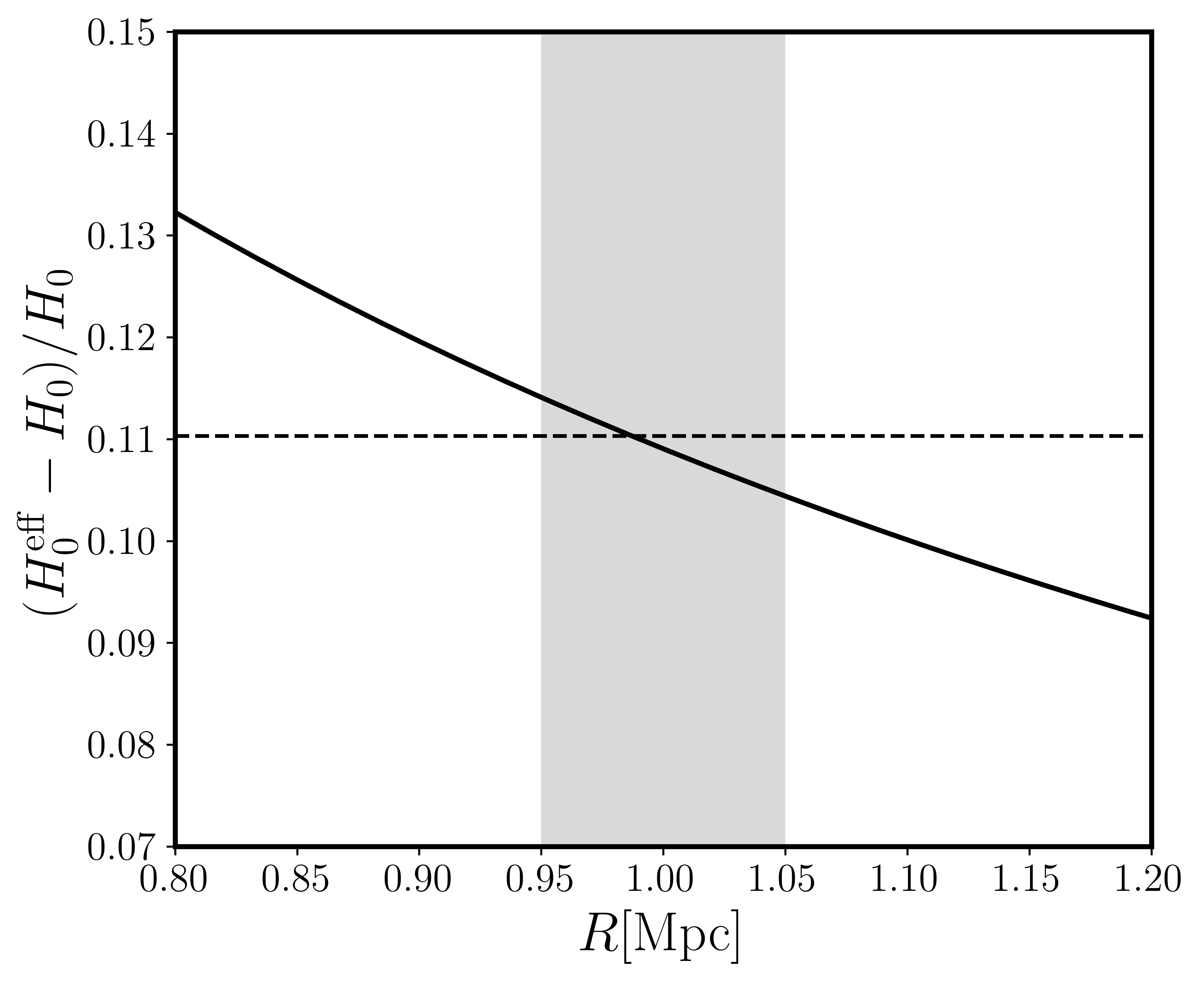
Refer to caption
Figure 6: We show the dependence of the fractional difference between the effective and global Hubble rates. Again the vertical grey area is a constraint on the radius of the zero-velocity surface that separates our local group from the Hubble flow 1999A&ARv…9..273V; Li:2007eg; Karachentsev:2008st. The vertical axis is an absolute value of the difference.

The fractional change in the area distance has already been discussed in sub-section II.3 and the key results shown in figure 3, hence we focus on the fractional difference between the effective and the global Hubble rate:

H0eff−H0H0=−445​f2​(0)​σR2.\frac{{H^{\rm{eff}}_{0}}-{H_{0}}}{{H_{0}}}=-\frac{4}{45}f^{2}(0)\sigma^{2}_{R}\,. (110)

We plot equation (110) in figure 6 as a function of the smoothing scale. Note that H0H_{0} is the Hubble rate measured by the local distance ladder technique. We find about (8−12)%(8-12)\% change to the Hubble rate when the tidal field is smoothed at the zero-velocity surface of our local group.

IV Conclusion

We showed how to derive a very concise expression for the area distance in a lumpy universe. This approach makes it easier and straightforward to analytically isolate and estimate the impact of the general relativistic corrections to the multipole moments of the area distance when compared to the perturbation of the full null focusing equation Umeh:2012pn; Umeh:2014ana To obtain this simplified view-point, we made use of the general coordinate transformation to derive a relationship between the source position and the image position. The relative difference between these positions can also be expressed in terms of the deviation vector when the image position is identified as the position of the central ray. We showed how to perform an irreducible decomposition of the Jacobian of the transformation with respect to the line of sight direction of the observer. This decomposition scheme follows the “Cosmic Ruler” decomposition approach introduced in Schmidt:2012ne. The orthogonal component of the deviation vector leads to the traditional Weak gravitational lensing parameters while the contribution of radial component in the Jacobian projected unto the screen space leads to the radial lensing correction/effect that we studied further. On the surface of constant redshift, the radial component is sourced by the perturbation in the observed source redshift. On the constant redshift surface, the radial lensing effects is known as the Doppler lensing effects and we showed that the leading order part is the parallax effect. That is the displacement in the background source position due to the relative velocity of the observer. We showed how to evaluate the impact of the parallax effect on the monopole of the area distance and the distance modulus.

In order to calculate correctly the impact of the parallax effect on the monopole of the area distance, we needed a model of the heliocentric peculiar velocity. The heliocentric peculiar velocity cannot be calculated within our cosmological perturbation theory scheme Macaulay:2011av. Therefore, to maintain consistency, we positioned the observer at the barycenter of our local group, this allows us to use the techniques developed in the study of the CMB temperature anisotropies to perform a full sky spherical harmonic decomposition of the correction to the area distance. We discussed how to perform this calculation in greater detail in Appendix C. The benefit of this approach is that the contribution of the heliocentric peculiar velocity can easily be included by boosting to the heliocentric frame when the correct heliocentric peculiar velocity is determined. The impact of the heliocentric peculiar velocity on the luminosity distance was studied in Kaiser:2014jca.

Similarly, when calculating the area distance using the general coordinate transformation approach or using the focusing equation (Sachs equation or the geodesic deviation equation of the Jacobi equation) we are in principle assuming that the observer and the source are connected by a one-parameter family geodesics. This does not hold in our universe because there exists a conjugate point at the boundary of our local group Nicolaescubook; Dalal:2020mjw. The focusing equation or the coordinate system induced by a one-parameter family of geodesics breaks down at a conjugate point Witten:2019qhl. Therefore to go beyond the conjugate point, another set of coordinate systems needs to the introduced. In order to avoid these complications, we analytically continued the monopole of the area distance as a function of the cosmological redshift beyond the conjugate point and then use a top-hat window function to smooth over divergent modes at the scale RR. We showed that the smoothing scale RR is given by the radius of the zero-velocity surface. What this means is that we can trust the perturbation theory prediction up the scale RR. Using the constraint on the cosmological parameters given by the Planck’s experiment Aghanim:2018eyx, we showed that the contribution of the inhomogeneities to the background area distance(or the the luminosity distance) at low redshift (zcut≤z≤0.001z_{\rm{cut}}\leq z\leq 0.001) could range from (4-12)%. Here the zcutz_{\rm{cut}} is determined by the radius of the zero-velocity surface(see equation (63) for details).

In addition, we studied the consequences of the modification to the monopole of the area distance in the low redshift limit on the cosmic distance ladder or the first rung of the distance ladder. We showed that the distance to nearby sources are impacted by the tidal deformation. The distance to the anchors used for the calibration of the absolute magnitude of the SNIa are located in the region where the impact of the tidal deformation cannot be neglected. Also, since distance is a two-point function, even sources far away in the Hubble flow are affected via the calibration of the absolute magnitude. We showed how the impact of the tidal deformation could bias the calibration of the SNIa absolute magnitude and we argue that it provides a natural explanation to the SNIa absolute magnitude tension. That is it explains the difference between the SNIa absolute magnitude determined using local distance anchors and the absolute magnitude obtained by inverse distance ladder with the proper length of the sound horizon at the last scattering surface as an anchor. Using the Alcock-Paczynski parameters as observables we showed that the inferred Hubble rate from the BAO measurement under-estimates the Hubble rate of an expanding universe by about (8-12)%. This is exactly the amount required to resolve the Hubble tension DiValentino:2021izs.

Finally, we neglected the impact of the heliocentric peculiar velocity on the luminosity distance or the apparent magnitude. It is important to note that including this coordinate dependent correction will not impact our result on the supernova absolute magnitude tension or the Hubble tension. We expect that the heliocentric peculiar velocity will impact the position of the intercept of the Hubble diagram. We shall study this in detail elsewhere.

Acknowledgement

I benefited immensely from discussions with Chris Clarkson, Robert Crittenden, Emir Gumrukcuoglu, Pierre Fleury, Asta Heinesen, Mathew Hull, Antony Lewis, Kazuya Koyama and Daniela Saadeh. The works by G.F.R. Ellis on this topic have been very crucial. I am supported by the UK Science & Technology Facilities Council (STFC) Consolidated Grants Grant ST/S000550/1 and the South African Square Kilometre Array Project. The perturbation theory computations in this paper were done with the help of tensor algebra software xPand Pitrou:2013hga which is based on xPert Brizuela:2008ra.

Data Access Statement

No new data were generated or analysed in support of this research

Appendix A Physical Position from perturbed background

We derive the full expression for the source position by solving the photon geodesic equation

k^b​∇^b​k^a=0.\displaystyle\hat{k}^{b}\hat{\nabla}_{b}\hat{k}^{a}=0\,. (111)

Following Sachs and Wolfe Sachs:1967er, the conformal transformation g^a​b→ga​b\hat{g}_{ab}\rightarrow g_{ab} maps the null geodesic equation associated with the physical metric g^a​b\hat{g}_{ab} (perturbed FLRW metric) to a null geodesic equation derived from a perturbed Minkowski metric ga​bg_{ab}. Both metrics are related according to ga​b=a−2​g^a​bg_{ab}=a^{-2}\hat{g}_{ab}. The contravariant photon 4-vector transforms as k^b=a−2​kb\hat{k}^{b}=a^{-2}k^{b} while the covariant photon 4-vector transforms as k^a=ka\hat{k}_{a}=k_{a}. The affine parameters transform as d​λ^→d​λ=a−2​d​λ^{\rm{d}}\hat{\lambda}\rightarrow{\rm{d}}\lambda=a^{-2}{\rm{d}}\hat{\lambda}. A given time-like 4-velocity, u^a\hat{u}^{a} on the physical spacetime, it transforms as u^a=a−1​ua⇔u^a=a​ua\hat{u}^{a}=a^{-1}u^{a}\Leftrightarrow\hat{u}_{a}=au_{a}. The photon energy transforms as E^=−u^b​k^b=−a−1​ub​kb=a−1​E\hat{E}=-\hat{u}_{b}\hat{k}^{b}=-a^{-1}\,u_{b}k^{b}=a^{-1}E.

This implies that we can compute the photon energy on a perturbed Minkowski space-time and simply multiply the conformal factor to obtain the corresponding expression in the physical spacetime. Similarly, we can compute the source position using the perturbations of the Minkowski metric, then multiply by the scale factor to obtain the equivalent in an expanding spacetime. The solution to the geodesic equation on a perturbed Minkowski metric is given by Umeh:2012pn

δ(1)​k0\displaystyle\delta^{\text{\tiny\color[rgb]{1,0,0}{({{1}})}}}k^{0} =\displaystyle= −2​(Φs(1)−Φo(1))+2​∫λoλsΦ(1)′​𝑑λ,\displaystyle-2(\Phi^{\text{\tiny\color[rgb]{1,0,0}{({{1}})}}}_{s}-\Phi^{\text{\tiny\color[rgb]{1,0,0}{({{1}})}}}_{o})+2\int_{\lambda_{o}}^{\lambda_{s}}{\Phi^{\text{\tiny\color[rgb]{1,0,0}{({{1}})}}}}^{\prime}{\rm{d}}\lambda\,, (112)
δ(1)​k∥\displaystyle\delta^{\text{\tiny\color[rgb]{1,0,0}{({{1}})}}}k_{{\text{\tiny$\|$}}} =\displaystyle= −2∫λoλsΦ(1)′dλ,\displaystyle-2\int_{\lambda_{o}}^{\lambda_{s}}{\Phi^{\text{\tiny\color[rgb]{1,0,0}{({{1}})}}}}^{\prime}{\rm{d}}\lambda\,, (113)
δ(1)​k⊥i\displaystyle\delta^{\text{\tiny\color[rgb]{1,0,0}{({{1}})}}}k_{\bot}^{i} =\displaystyle= −2∫λoλs∇i⊥Φ(1)dλ.\displaystyle-2\int_{\lambda_{o}}^{\lambda_{s}}\nabla^{i}_{\bot}{\Phi^{\text{\tiny\color[rgb]{1,0,0}{({{1}})}}}}{\rm{d}}\lambda\,. (114)

At second order we considered only the dominant terms.

δ(2)​k0\displaystyle\delta^{\text{\tiny\color[rgb]{0,1,0}{({{2}})}}}k^{0} ≈\displaystyle\approx −2​Φs(2)+∫λoλs(Φ(2)′+Ψ(2)′)​𝑑λ+8​∫∫(λo−λ~)(λo−λ)​∇⊥iΦ(1)′​(λ~)​∫∇⊥iΦ(1)​(λ~),\displaystyle-2\Phi^{\text{\tiny\color[rgb]{0,1,0}{({{2}})}}}_{s}+\int_{\lambda_{o}}^{\lambda_{s}}\left({\Phi^{\text{\tiny\color[rgb]{0,1,0}{({{2}})}}}}^{\prime}+{\Psi^{\text{\tiny\color[rgb]{0,1,0}{({{2}})}}}}^{\prime}\right){\rm{d}}\lambda+8\int\int\frac{(\lambda_{o}-\tilde{\lambda})}{(\lambda_{o}-\lambda)}\nabla_{\bot}^{i}{\Phi^{\text{\tiny\color[rgb]{1,0,0}{({{1}})}}}}^{\prime}(\tilde{\lambda})\int\nabla_{\bot i}{\Phi^{\text{\tiny\color[rgb]{1,0,0}{({{1}})}}}}(\tilde{\lambda})\,, (115)
δ(2)k∥\displaystyle\delta^{\text{\tiny\color[rgb]{0,1,0}{({{2}})}}}k_{{}_{{\text{\tiny$\|$}}}} ≈\displaystyle\approx −∫λoλs(Φ(2)′+Ψ(2)′)dλ+8∫∇⊥iΦ(1)∫∇⊥iΦ(1)(λ~)−∫∫(λo−λ~)(λo−λ)∇⊥iΦ(1)′(λ~)∫∇⊥iΦ(1)(λ~)\displaystyle-\int_{\lambda_{o}}^{\lambda_{s}}\left({\Phi^{\text{\tiny\color[rgb]{0,1,0}{({{2}})}}}}^{\prime}+{\Psi^{\text{\tiny\color[rgb]{0,1,0}{({{2}})}}}}^{\prime}\right){\rm{d}}\lambda+8\int\nabla_{\bot}^{i}{\Phi^{\text{\tiny\color[rgb]{1,0,0}{({{1}})}}}}\int\nabla_{\bot i}{\Phi^{\text{\tiny\color[rgb]{1,0,0}{({{1}})}}}}(\tilde{\lambda})-\int\int\frac{(\lambda_{o}-\tilde{\lambda})}{(\lambda_{o}-\lambda)}\nabla_{\bot}^{i}{\Phi^{\text{\tiny\color[rgb]{1,0,0}{({{1}})}}}}^{\prime}(\tilde{\lambda})\int\nabla_{\bot i}{\Phi^{\text{\tiny\color[rgb]{1,0,0}{({{1}})}}}}(\tilde{\lambda}) (116)
δ(2)​k⊥i\displaystyle\delta^{\text{\tiny\color[rgb]{0,1,0}{({{2}})}}}k_{\bot}^{i} ≃\displaystyle\simeq −∫λoλs∇⊥i(Φ(2)+Ψ(2))dλ\displaystyle-\int_{\lambda_{o}}^{\lambda_{s}}\nabla^{i}_{\bot}\left(\Phi^{\text{\tiny\color[rgb]{0,1,0}{({{2}})}}}+\Psi^{\text{\tiny\color[rgb]{0,1,0}{({{2}})}}}\right){\rm{d}}\lambda (117)
+2∫λoλs[∫λoλ∇⊥j(Φ(1)(λ~)+Ψ(1)(λ~))dλ~∫λoλr~r∇⊥j∇⊥i(Φ(1)(λ~)+Ψ(1)(λ~))dλ~]dλ.\displaystyle+2\int_{\lambda_{o}}^{\lambda_{s}}\left[\int_{\lambda_{o}}^{\lambda}\nabla_{\bot}^{j}\left(\Phi^{\text{\tiny\color[rgb]{1,0,0}{({{1}})}}}(\tilde{\lambda})+\Psi^{\text{\tiny\color[rgb]{1,0,0}{({{1}})}}}(\tilde{\lambda})\right){\rm{d}}\tilde{\lambda}\int_{\lambda_{o}}^{\lambda}\frac{\tilde{r}}{r}\nabla_{\bot j}\nabla_{\bot}^{i}\left(\Phi^{\text{\tiny\color[rgb]{1,0,0}{({{1}})}}}(\tilde{\lambda})+\Psi^{\text{\tiny\color[rgb]{1,0,0}{({{1}})}}}(\tilde{\lambda})\right){\rm{d}}\tilde{\lambda}\right]{\rm{d}}\lambda\,. (118)

The full expression is given in Umeh:2012pn. The perturbed photon trajectory is obtain by integrating equations (115) and (118)

δ(1)​η​(η¯s,𝐧^)\displaystyle\delta^{\text{\tiny\color[rgb]{1,0,0}{({{1}})}}}{\eta}(\bar{\eta}_{s},{{\bf\hat{n}}}) =\displaystyle= 2​∫0rs(rs−r)​Φ(1)′​𝑑r\displaystyle 2\int_{0}^{r_{s}}(r_{s}-r){\Phi^{\text{\tiny\color[rgb]{1,0,0}{({{1}})}}}}^{\prime}{\rm{d}}r (119)
δ(1)​x∥​(η¯s,𝐧^)\displaystyle\delta^{\text{\tiny\color[rgb]{1,0,0}{({{1}})}}}x_{{\text{\tiny$\|$}}}(\bar{\eta}_{s},{{\bf\hat{n}}}) ≈\displaystyle\approx −2∫rs0Φ(1)dr,\displaystyle-2\int^{r_{s}}_{0}\Phi^{\text{\tiny\color[rgb]{1,0,0}{({{1}})}}}{\rm{d}}r\,, (120)
δ(1)​x⊥i​(η¯s,𝐧^)\displaystyle\delta^{\text{\tiny\color[rgb]{1,0,0}{({{1}})}}}x^{i}_{\bot}(\bar{\eta}_{s},{{\bf\hat{n}}}) =\displaystyle= ∫0rs(r−rs)​∇⊥i(Φ(1)+Ψ(1))​𝑑r,\displaystyle\int^{r_{s}}_{0}{(r-r_{s})}\nabla_{\bot}^{i}(\Phi^{\text{\tiny\color[rgb]{1,0,0}{({{1}})}}}+\Psi^{\text{\tiny\color[rgb]{1,0,0}{({{1}})}}}){\rm{d}}r\,, (121)

where we have defined r=ηo−η¯r=\eta_{o}-\bar{\eta}. At second order, we need only the radial component

δ(2)x∥(λs,𝐧^)\displaystyle\delta^{\text{\tiny\color[rgb]{0,1,0}{({{2}})}}}x_{{}_{{\text{\tiny$\|$}}}}(\lambda_{s},{{\bf\hat{n}}}) =\displaystyle= −∫0rs(Φ(2)+Ψ(2))dr+8∫0rsdr′∫0r′dr′′(rs−r′)∇⊥iΦ(1)(r′𝐧^)∇⊥iΦ(1)(r′′𝐧^)\displaystyle-\int^{r_{s}}_{0}\left(\Phi^{\text{\tiny\color[rgb]{0,1,0}{({{2}})}}}+\Psi^{\text{\tiny\color[rgb]{0,1,0}{({{2}})}}}\right){\rm{d}}r+8\int_{0}^{r_{s}}{\rm{d}}r^{\prime}\int_{0}^{r^{\prime}}{\rm{d}}r^{\prime\prime}(r_{s}-r^{\prime})\nabla_{\bot i}\Phi^{\text{\tiny\color[rgb]{1,0,0}{({{1}})}}}(r^{\prime}{{\bf\hat{n}}})\nabla_{\bot}^{i}\Phi^{\text{\tiny\color[rgb]{1,0,0}{({{1}})}}}(r^{\prime\prime}{{\bf\hat{n}}}) (122)
+8∫0rsdr∫0rdr′∫0rdr′′r′′r∇⊥iΦ(1)(r′𝐧^)∇⊥iΦ(1)(r′′𝐧^).\displaystyle+8\int_{0}^{r_{s}}{\rm{d}}r\int_{0}^{r}{\rm{d}}r^{\prime}\int_{0}^{r}{\rm{d}}r^{\prime\prime}\frac{r^{\prime\prime}}{r}\nabla_{\bot i}\Phi^{\text{\tiny\color[rgb]{1,0,0}{({{1}})}}}(r^{\prime}{{\bf\hat{n}}})\nabla_{\bot}^{i}\Phi^{\text{\tiny\color[rgb]{1,0,0}{({{1}})}}}(r^{\prime\prime}{{\bf\hat{n}}})\,.

Together, we find that the source position as function of the Minkowski background spacetime is given by

xi​(η¯,𝒙¯)\displaystyle x^{i}(\bar{\eta},\bar{\bm{x}}) =\displaystyle= x¯i​(η¯)+δ(1)​xi​(η¯,𝒙¯)+12​δ(2)​xi​(η¯,𝒙¯)+𝒪⁡(ϵ3),\displaystyle\bar{x}^{i}(\bar{\eta})+\delta^{\text{\tiny\color[rgb]{1,0,0}{({{1}})}}}x^{i}(\bar{\eta},\bar{\bm{x}})+\frac{1}{2}\delta^{\text{\tiny\color[rgb]{0,1,0}{({{2}})}}}x^{i}(\bar{\eta},\bar{\bm{x}})+\mathcal{O}(\epsilon^{3})\,, (123)

where η¯\bar{\eta} and x¯i\bar{x}^{i} are the background conformal time and spatial coordinate position respectively. Up to this point, the perturbations live on the background spacetime, but, light rays travel on physical spacetime, not on the background spacetime. Firstly, we need to express equation (123) in terms of the affine parameter of the full spacetime. On the background spacetime, we have

d​η¯d​λ¯=1,d​x¯id​λ¯=−ni.\frac{{\rm{d}}\bar{\eta}}{{\rm{d}}\bar{\lambda}}=1\,,\qquad\frac{{\rm{d}}\bar{x}^{i}}{{\rm{d}}\bar{\lambda}}=-n^{i}\,. (124)

Again nin^{i} is the LoS direction vector. Integrating these two equations from the observer to the source give: x¯i=−ni​(λ¯s−λo)=ni​r\bar{x}^{i}=-n^{i}(\bar{\lambda}_{s}-\lambda_{o})=n^{i}r with r=(λo−λ¯s)=(ηo−η¯s)r=(\lambda_{o}-\bar{\lambda}_{s})=(\eta_{o}-\bar{\eta}_{s}). Given that λ=λ¯+δ(1)​λ+δ(2)​λ/2\lambda=\bar{\lambda}+\delta^{\text{\tiny\color[rgb]{1,0,0}{({{1}})}}}\lambda+\delta^{\text{\tiny\color[rgb]{0,1,0}{({{2}})}}}\lambda/2 we re-map x¯i\bar{x}^{i} to the affine parameter associated with the perturbed Minkowski spacetime

x¯i​(η¯)→x¯i​(λ)−δ(1)​λ​d​xid​λ|s−12​((δ(1)​λ)2​d2​xid​λ2|s+δ(2)​λ​d​xid​λ|s)+𝒪⁡(ϵ3).\displaystyle\bar{x}^{i}(\bar{\eta})\rightarrow\bar{x}^{i}(\lambda)-\delta^{\text{\tiny\color[rgb]{1,0,0}{({{1}})}}}\lambda\frac{{\rm{d}}x^{i}}{{\rm{d}}\lambda}\bigg|_{s}-\frac{1}{2}\left(\left(\delta^{\text{\tiny\color[rgb]{1,0,0}{({{1}})}}}\lambda\right)^{2}\frac{{\rm{d}}^{2}x^{i}}{{\rm{d}}\lambda^{2}}\bigg|_{s}+\delta^{\text{\tiny\color[rgb]{0,1,0}{({{2}})}}}\lambda\frac{{\rm{d}}x^{i}}{{\rm{d}}\lambda}\bigg|_{s}\right)+\mathcal{O}(\epsilon^{3})\,. (125)

Since nin^{i} is constant on the background, its acceleration vanishes d2​xi/d​λ2|s=0{{\rm{d}}^{2}x^{i}}/{{\rm{d}}\lambda^{2}}|_{s}=0, therefore

x¯i​(η¯)→r​ni+δ(1)​λ​ni+12​δ(2)​λ​ni+𝒪⁡(ϵ3).\displaystyle\bar{x}^{i}(\bar{\eta})\rightarrow rn^{i}+\delta^{\text{\tiny\color[rgb]{1,0,0}{({{1}})}}}\lambda n^{i}+\frac{1}{2}\delta^{\text{\tiny\color[rgb]{0,1,0}{({{2}})}}}\lambda n^{i}+\mathcal{O}(\epsilon^{3})\,. (126)

This implies that the perturbed position given in equation (123) may be written in terms of λs\lambda_{s} by replacing x¯i​(η)\bar{x}^{i}({\eta})

xi​(λ,𝐧^)\displaystyle x^{i}(\lambda,{{\bf\hat{n}}}) =\displaystyle= x¯i​(λ)+[δ(1)​xi+nsi​δ(1)​λ]+12​[δ(2)​xi+nsi​δ(2)​λ].\displaystyle\bar{x}^{i}(\lambda)+\left[\delta^{\text{\tiny\color[rgb]{1,0,0}{({{1}})}}}x^{i}+{n^{i}_{s}}\delta^{\text{\tiny\color[rgb]{1,0,0}{({{1}})}}}\lambda\right]+\frac{1}{2}\left[\delta^{\text{\tiny\color[rgb]{0,1,0}{({{2}})}}}x^{i}+n^{i}_{s}\delta^{\text{\tiny\color[rgb]{0,1,0}{({{2}})}}}\lambda\right]\,. (127)

Similarly, at first order, we re-map the conformal time and position

δ(1)​λ​(η¯,𝒙¯)\displaystyle\delta^{\text{\tiny\color[rgb]{1,0,0}{({{1}})}}}\lambda(\bar{\eta},\bar{\bm{x}}) ≈\displaystyle\approx δ(1)λ(λ,𝐧^)−Δ(1)x∥(η¯,𝒙¯)∂∥δ(1)λ(η¯,𝒙¯)−δ(1)x⊥i(η¯,𝒙¯)∇⊥iδ(1)λ(η¯,𝐧^),\displaystyle\delta^{\text{\tiny\color[rgb]{1,0,0}{({{1}})}}}\lambda({\lambda},{{\bf\hat{n}}})-\Delta^{\text{\tiny\color[rgb]{1,0,0}{({{1}})}}}x_{{}_{{\text{\tiny$\|$}}}}(\bar{\eta},\bar{\bm{x}})\partial_{{}_{{\text{\tiny$\|$}}}}\delta^{\text{\tiny\color[rgb]{1,0,0}{({{1}})}}}\lambda(\bar{\eta},\bar{\bm{x}})-\delta^{\text{\tiny\color[rgb]{1,0,0}{({{1}})}}}x_{\bot}^{i}(\bar{\eta},\bar{\bm{x}})\nabla_{\bot i}\delta^{\text{\tiny\color[rgb]{1,0,0}{({{1}})}}}\lambda(\bar{\eta},{{\bf\hat{n}}})\,, (128)
δ(1)x∥(η¯,𝒙¯)\displaystyle\delta^{\text{\tiny\color[rgb]{1,0,0}{({{1}})}}}x_{{}_{{\text{\tiny$\|$}}}}(\bar{\eta},\bar{\bm{x}}) ≈\displaystyle\approx δ(1)x∥(λ,𝐧^)−Δ(1)x∥(η¯,𝒙¯)∂∥δ(1)x∥(η¯,𝒙¯)−δ(1)x⊥i(η¯,𝒙¯)∇⊥iδ(1)x∥(η¯,𝐧^),\displaystyle\delta^{\text{\tiny\color[rgb]{1,0,0}{({{1}})}}}x_{{}_{{\text{\tiny$\|$}}}}({\lambda},{{\bf\hat{n}}})-\Delta^{\text{\tiny\color[rgb]{1,0,0}{({{1}})}}}x_{{}_{{\text{\tiny$\|$}}}}(\bar{\eta},\bar{\bm{x}})\partial_{{}_{{\text{\tiny$\|$}}}}\delta^{\text{\tiny\color[rgb]{1,0,0}{({{1}})}}}x_{{}_{{\text{\tiny$\|$}}}}(\bar{\eta},\bar{\bm{x}})-\delta^{\text{\tiny\color[rgb]{1,0,0}{({{1}})}}}x_{\bot}^{i}(\bar{\eta},\bar{\bm{x}})\nabla_{\bot i}\delta^{\text{\tiny\color[rgb]{1,0,0}{({{1}})}}}x_{{}_{{\text{\tiny$\|$}}}}(\bar{\eta},{{\bf\hat{n}}})\,, (129)
δ(1)​x⊥i​(η¯,𝒙¯)\displaystyle\delta^{\text{\tiny\color[rgb]{1,0,0}{({{1}})}}}x^{i}_{\bot}(\bar{\eta},\bar{\bm{x}}) ≈\displaystyle\approx δ(1)​x⊥i​(λ,𝐧^)−δ(1)​x⊥i​(η¯,𝐧^)​∇⊥iδ(1)​x⊥i​(η¯,𝐧^).\displaystyle\delta^{\text{\tiny\color[rgb]{1,0,0}{({{1}})}}}x^{i}_{\bot}(\lambda,{{\bf\hat{n}}})-\delta^{\text{\tiny\color[rgb]{1,0,0}{({{1}})}}}x_{\bot}^{i}(\bar{\eta},{{\bf\hat{n}}})\nabla_{\bot i}\delta^{\text{\tiny\color[rgb]{1,0,0}{({{1}})}}}x^{i}_{\bot}(\bar{\eta},{{\bf\hat{n}}})\,. (130)

Again, we focused on the dominant terms only. Substituting these terms in equation (127) gives

xi​(λ,𝐧^)\displaystyle x^{i}(\lambda,{{\bf\hat{n}}}) =\displaystyle= x¯i(λ)+[δ(1)x⊥i+nsi(δ(1)x∥+δ(1)λ)]+12[δ(2)x⊥i−2δ(1)x⊥i∇⊥iδ(1)x⊥i\displaystyle\bar{x}^{i}(\lambda)+\left[\delta^{\text{\tiny\color[rgb]{1,0,0}{({{1}})}}}x^{i}_{\bot}+{n^{i}_{s}}\left(\delta^{\text{\tiny\color[rgb]{1,0,0}{({{1}})}}}x_{{}_{{\text{\tiny$\|$}}}}+\delta^{\text{\tiny\color[rgb]{1,0,0}{({{1}})}}}\lambda\right)\right]+\frac{1}{2}\bigg[\delta^{\text{\tiny\color[rgb]{0,1,0}{({{2}})}}}x^{i}_{\bot}-2\delta^{\text{\tiny\color[rgb]{1,0,0}{({{1}})}}}x_{\bot}^{i}\nabla_{\bot i}\delta^{\text{\tiny\color[rgb]{1,0,0}{({{1}})}}}x^{i}_{\bot} (131)
+nsi(δ(2)x∥+δ(2)λ−2Δ(1)x∥(∂∥δ(1)λ+∂∥δ(1)x∥)−2δ(1)x⊥i(∇⊥iδ(1)λ+∇⊥iδ(1)λ))].\displaystyle+n^{i}_{s}\left(\delta^{\text{\tiny\color[rgb]{0,1,0}{({{2}})}}}x_{{}_{{\text{\tiny$\|$}}}}+\delta^{\text{\tiny\color[rgb]{0,1,0}{({{2}})}}}\lambda-2\Delta^{\text{\tiny\color[rgb]{1,0,0}{({{1}})}}}x_{{}_{{\text{\tiny$\|$}}}}\left(\partial_{{}_{{\text{\tiny$\|$}}}}\delta^{\text{\tiny\color[rgb]{1,0,0}{({{1}})}}}\lambda+\partial_{{}_{{\text{\tiny$\|$}}}}\delta^{\text{\tiny\color[rgb]{1,0,0}{({{1}})}}}x_{{}_{{\text{\tiny$\|$}}}}\right)-2\delta^{\text{\tiny\color[rgb]{1,0,0}{({{1}})}}}x_{\bot}^{i}\left(\nabla_{\bot i}\delta^{\text{\tiny\color[rgb]{1,0,0}{({{1}})}}}\lambda+\nabla_{\bot i}\delta^{\text{\tiny\color[rgb]{1,0,0}{({{1}})}}}\lambda\right)\right)\bigg]\,.

where Δ(1)x∥=δ(1)x∥+δ(1)λ.\Delta^{\text{\tiny\color[rgb]{1,0,0}{({{1}})}}}x_{{}_{{\text{\tiny$\|$}}}}=\delta^{\text{\tiny\color[rgb]{1,0,0}{({{1}})}}}x_{{}_{{\text{\tiny$\|$}}}}+\delta^{\text{\tiny\color[rgb]{1,0,0}{({{1}})}}}\lambda\,. The corresponding position on the perturbed FLRW spacetime is given by xFLRWi​(λ,𝐧^)=a⁡(η¯)​xi​(λ,𝐧^)x^{i}_{\rm{FLRW}}(\lambda,{{\bf\hat{n}}})=a(\bar{\eta})x^{i}(\lambda,{{\bf\hat{n}}}). Therefore, we need to re-map the conformal factor

a⁡(η¯)\displaystyle a(\bar{\eta}) =\displaystyle= a(λs)[1−ℋsδ(1)λ−12ℋs(δ(2)λ−2Δ(1)x∥∂∥δ(1)λ−2δ(1)x⊥i∇⊥iδ(1)λ+(ℋ′ℋs+ℋs)(δ(1)λ)2)],\displaystyle a(\lambda_{s})\left[1-\mathcal{H}\,_{s}\delta^{\text{\tiny\color[rgb]{1,0,0}{({{1}})}}}\lambda-\frac{1}{2}\mathcal{H}\,_{s}\left(\,{\delta}^{\text{\tiny\color[rgb]{0,1,0}{({{2}})}}}\lambda-2\Delta^{\text{\tiny\color[rgb]{1,0,0}{({{1}})}}}x_{{}_{{\text{\tiny$\|$}}}}\partial_{{}_{{\text{\tiny$\|$}}}}\delta^{\text{\tiny\color[rgb]{1,0,0}{({{1}})}}}\lambda-2\delta^{\text{\tiny\color[rgb]{1,0,0}{({{1}})}}}x_{\bot}^{i}\nabla_{\bot i}\delta^{\text{\tiny\color[rgb]{1,0,0}{({{1}})}}}\lambda+\left(\frac{\mathcal{H}\,^{\prime}}{\mathcal{H}\,_{s}}+\mathcal{H}\,_{s}\right)(\delta^{\text{\tiny\color[rgb]{1,0,0}{({{1}})}}}\lambda)^{2}\right)\right]\,, (132)

Putting equation (132) into xFLRWi​(λ,𝐧^)=a⁡(η¯)​xi​(λ,𝐧^)x^{i}_{\rm{FLRW}}(\lambda,{{\bf\hat{n}}})=a(\bar{\eta})x^{i}(\lambda,{{\bf\hat{n}}}) and using equation (131) we find

xFLRWi​(λs,𝐧^)\displaystyle x^{i}_{\rm{FLRW}}(\lambda_{s},{{\bf\hat{n}}}) ≈\displaystyle\approx a(λs)rs{ni+[δ(1)​x⊥irs+[δ(1)x∥rs−(1−1rs​ℋs)ℋδ(1)λ]ni]\displaystyle a(\lambda_{s})r_{s}\bigg\{{n}^{i}+\left[\frac{\delta^{\text{\tiny\color[rgb]{1,0,0}{({{1}})}}}x^{i}_{\bot}}{r_{s}}+\left[\frac{\delta^{\text{\tiny\color[rgb]{1,0,0}{({{1}})}}}x_{{}_{{\text{\tiny$\|$}}}}}{r_{s}}-\left(1-\frac{1}{r_{s}\mathcal{H}\,_{s}}\right){\mathcal{H}\,}\delta^{\text{\tiny\color[rgb]{1,0,0}{({{1}})}}}\lambda\right]n^{i}\right] (133)
+12[δ(2)​x⊥irs−2rsΔ(1)x⊥j∇⊥jδ(1)x⊥i+(δ(2)x∥rs−2rsΔ(1)x∥∂∥δ(1)x∥\displaystyle+\frac{1}{2}\bigg[\frac{\delta^{\text{\tiny\color[rgb]{0,1,0}{({{2}})}}}x^{i}_{\bot}}{r_{s}}-\frac{2}{r_{s}}\Delta^{\text{\tiny\color[rgb]{1,0,0}{({{1}})}}}x^{j}_{\bot}\nabla_{\bot j}\delta^{\text{\tiny\color[rgb]{1,0,0}{({{1}})}}}x^{i}_{\bot}+\bigg(\frac{\delta^{\text{\tiny\color[rgb]{0,1,0}{({{2}})}}}x_{{}_{{\text{\tiny$\|$}}}}}{r_{s}}-\frac{2}{r_{s}}\Delta^{\text{\tiny\color[rgb]{1,0,0}{({{1}})}}}x_{{}_{{\text{\tiny$\|$}}}}\partial_{{}_{{\text{\tiny$\|$}}}}\delta^{\text{\tiny\color[rgb]{1,0,0}{({{1}})}}}x_{{}_{{\text{\tiny$\|$}}}}
−2rsδ(1)x⊥i∇⊥iδ(1)δx∥−(1−1rs​ℋs)ℋ(δ(2)λ−2Δ(1)x∥∂∥δ(1)λ−2δ(1)x⊥j∇⊥jδ(1)λ))ni]},\displaystyle-\frac{2}{r_{s}}\delta^{\text{\tiny\color[rgb]{1,0,0}{({{1}})}}}x_{\bot}^{i}\nabla_{\bot i}\delta^{\text{\tiny\color[rgb]{1,0,0}{({{1}})}}}\delta x_{{}_{{\text{\tiny$\|$}}}}-\left(1-\frac{1}{r_{s}\mathcal{H}\,_{s}}\right){\mathcal{H}\,}\left(\delta^{\text{\tiny\color[rgb]{0,1,0}{({{2}})}}}\lambda-2\Delta^{\text{\tiny\color[rgb]{1,0,0}{({{1}})}}}x_{{}_{{\text{\tiny$\|$}}}}\partial_{{}_{{\text{\tiny$\|$}}}}\delta^{\text{\tiny\color[rgb]{1,0,0}{({{1}})}}}\lambda-2\delta^{\text{\tiny\color[rgb]{1,0,0}{({{1}})}}}x^{j}_{\bot}\nabla_{\bot j}\delta^{\text{\tiny\color[rgb]{1,0,0}{({{1}})}}}\lambda\right)\bigg)n^{i}\bigg]\bigg\}\,,

At this point, we can define the deviation vector

ξi​(λs,r​𝐧^)a⁡(λs)​rs\displaystyle\frac{{{\xi}^{i}(\lambda_{s},r{{\bf\hat{n}}})}}{a(\lambda_{s})r_{s}} =\displaystyle= xFLRWi​(λs,r​𝐧^)−x¯FLRWi​(λs)a⁡(λ)​rs=xFLRWi​(λs,r​𝐧^)−x¯FLRWi​(λs)d¯A​(λ).\displaystyle\frac{{x^{i}_{\rm{FLRW}}(\lambda_{s},r{{\bf\hat{n}}})-\bar{x}^{i}_{\rm{FLRW}}(\lambda_{s})}}{a(\lambda)r_{s}}=\frac{{x^{i}_{\rm{FLRW}}(\lambda_{s},r{{\bf\hat{n}}})-\bar{x}^{i}_{\rm{FLRW}}(\lambda_{s})}}{\bar{d}_{A}(\lambda)}\,. (134)

We measure the redshift and angles and not the affine parameter. Therefore, we have to express the deviation vector in terms of the cosmological redshift. This implies that the contributions to the observed redshift due to Doppler effects, Sachs-Wolfe effect, integrated Sachs-Wolfe effects, etc are interpreted as displacements in the position of the source due to a local over-density. The distance to a source falling into a local over-density along the line of sight direction may appear shorter while sources moving away from the local over-density may appear stretched Bolejko:2012uj. The perturbation of the observed redshift is given by

(1+zobs)=EsEo=a⁡(η¯o)a⁡(η¯s)​[1+δ(1)​z+12​δ(2)​z].\displaystyle\left(1+z_{\rm{obs}}\right)=\frac{E_{s}}{E_{o}}=\frac{a({\bar{\eta}_{o}})}{a({\bar{\eta}_{s}})}\left[1+\delta^{\text{\tiny\color[rgb]{1,0,0}{({{1}})}}}z+\frac{1}{2}\delta^{\text{\tiny\color[rgb]{0,1,0}{({{2}})}}}z\right]\,. (135)

where δ(1)​z\delta^{\text{\tiny\color[rgb]{1,0,0}{({{1}})}}}z and δ(2)​z\delta^{\text{\tiny\color[rgb]{0,1,0}{({{2}})}}}z denotes the first and second order perturbations in redshift respectively. Using equation (132), we write equation (135) as

1(1+zobs)\displaystyle\frac{1}{(1+{z}_{\rm{obs}})} =\displaystyle= a⁡(λs)a⁡(λo)[1+(−ℋδ(1)λ−δ(1)z)\displaystyle\frac{a({\lambda_{s}})}{a({\lambda_{o}})}\bigg[1+\left(-\mathcal{H}\,\delta^{\text{\tiny\color[rgb]{1,0,0}{({{1}})}}}\lambda-\delta^{\text{\tiny\color[rgb]{1,0,0}{({{1}})}}}z\right) (136)
+12(−ℋδ(2)λ−δ(2)z+2(δ(1)z)2+2ℋδ(1)zδ(1)λ+(d​ℋd​λs+ℋ2)(δ(1)λ)2)+𝒪(ϵ3].\displaystyle+\frac{1}{2}\left(-\mathcal{H}\,\delta^{\text{\tiny\color[rgb]{0,1,0}{({{2}})}}}\lambda-\delta^{\text{\tiny\color[rgb]{0,1,0}{({{2}})}}}z+2(\delta^{\text{\tiny\color[rgb]{1,0,0}{({{1}})}}}z)^{2}+2\mathcal{H}\,\delta^{\text{\tiny\color[rgb]{1,0,0}{({{1}})}}}z\delta^{\text{\tiny\color[rgb]{1,0,0}{({{1}})}}}\lambda+\left(\frac{{\rm{d}}\mathcal{H}\,}{{\rm{d}}\lambda_{s}}+\mathcal{H}\,^{2}\right)(\delta^{\text{\tiny\color[rgb]{1,0,0}{({{1}})}}}\lambda)^{2}\right)+\mathcal{O}(\epsilon^{3}\bigg]\,.

Imposing that the redshift is entirely due to Hubble flow(constant redshift surface) implies that

δ(1)​λ\displaystyle\delta^{\text{\tiny\color[rgb]{1,0,0}{({{1}})}}}\lambda =\displaystyle= −δ(1)​zℋ,\displaystyle-\frac{\delta^{\text{\tiny\color[rgb]{1,0,0}{({{1}})}}}z}{\mathcal{H}\,}, (137)
δ(2)​λ\displaystyle\delta^{\text{\tiny\color[rgb]{0,1,0}{({{2}})}}}\lambda =\displaystyle= −1ℋ​[δ(2)​z−(δ(1)​z)2​(1+1ℋ2​d​ℋd​λs)].\displaystyle-\frac{1}{\mathcal{H}\,}\left[\delta^{\text{\tiny\color[rgb]{0,1,0}{({{2}})}}}z-(\delta^{\text{\tiny\color[rgb]{1,0,0}{({{1}})}}}z)^{2}\left(1+\frac{1}{\mathcal{H}\,^{2}}\frac{{\rm{d}}\mathcal{H}\,}{{\rm{d}}\lambda_{s}}\right)\right]\,. (138)

Putting equations equations (137) and (138) in equation (133) gives

ξ(1)∥(zs,r𝐧^)d¯A\displaystyle\frac{{{\xi}^{\text{\tiny\color[rgb]{1,0,0}{({{1}})}}}{{}_{{\text{\tiny$\|$}}}}(z_{s},r{{\bf\hat{n}}})}}{\bar{d}_{A}} =\displaystyle= δ(1)x∥rs+(1−1rs​ℋs)​δ(1)​z,\displaystyle\frac{\delta^{\text{\tiny\color[rgb]{1,0,0}{({{1}})}}}x_{{}_{{\text{\tiny$\|$}}}}}{r_{s}}+\left(1-\frac{1}{r_{s}\mathcal{H}\,_{s}}\right)\delta^{\text{\tiny\color[rgb]{1,0,0}{({{1}})}}}z\,, (139)
ξ(2)∥(zs,r𝐧^)d¯A\displaystyle\frac{{{\xi}^{\text{\tiny\color[rgb]{0,1,0}{({{2}})}}}{{}_{{\text{\tiny$\|$}}}}(z_{s},r{{\bf\hat{n}}})}}{\bar{d}_{A}} =\displaystyle= δ(2)x∥rs−2rsδ(1)x⊥i∇⊥iδ(1)δx∥+(1−1rs​ℋs)(δ(2)z−2δ(1)​zℋ∂∥δ(1)z−2δ(1)x⊥j∇⊥jδ(1)z).\displaystyle\frac{\delta^{\text{\tiny\color[rgb]{0,1,0}{({{2}})}}}x_{{}_{{\text{\tiny$\|$}}}}}{r_{s}}-\frac{2}{r_{s}}\delta^{\text{\tiny\color[rgb]{1,0,0}{({{1}})}}}x_{\bot}^{i}\nabla_{\bot i}\delta^{\text{\tiny\color[rgb]{1,0,0}{({{1}})}}}\delta x_{{}_{{\text{\tiny$\|$}}}}+\left(1-\frac{1}{r_{s}\mathcal{H}\,_{s}}\right)\left({\delta^{\text{\tiny\color[rgb]{0,1,0}{({{2}})}}}z}-{2}\frac{\delta^{\text{\tiny\color[rgb]{1,0,0}{({{1}})}}}z}{\mathcal{H}\,}\partial_{{\text{\tiny$\|$}}}\delta^{\text{\tiny\color[rgb]{1,0,0}{({{1}})}}}z-2\delta^{\text{\tiny\color[rgb]{1,0,0}{({{1}})}}}x^{j}_{\bot}\nabla_{\bot j}\delta^{\text{\tiny\color[rgb]{1,0,0}{({{1}})}}}z\right)\,. (140)

The perturbed redshift in conformal Newtonian gauge is given by

δ​z=(∂∥vs−∂∥vo)−(Φs−Φo)−∫0rs(Φ′+Ψ′)​𝑑r.\delta z=\left(\partial_{\|}{v_{s}}-\partial_{\|}v_{o}\right)-\left(\Phi_{s}-\Phi_{o}\right)-\int_{0}^{r_{s}}\left({\Phi}^{\prime}+{\Psi}^{\prime}\right){{\rm{d}}}r. (141)

Using equation (141) we find that the line of sight component of the deviation vector is given by

ξ(1)∥(zs,𝐧^)a⁡(z)​rs\displaystyle\frac{{{\xi}^{\text{\tiny\color[rgb]{1,0,0}{({{1}})}}}{{}_{{\text{\tiny$\|$}}}}(z_{s},{{\bf\hat{n}}})}}{a(z)r_{s}} =\displaystyle= (∂∥vs(1)−∂∥vo(1))​(1−1rs​ℋs),\displaystyle\left(\partial_{\|}{v^{\text{\tiny\color[rgb]{1,0,0}{({{1}})}}}_{s}}-\partial_{\|}v^{\text{\tiny\color[rgb]{1,0,0}{({{1}})}}}_{o}\right)\left(1-\frac{1}{r_{s}\mathcal{H}\,_{s}}\right)\,, (142)
ξ(2)∥(zs,𝐧^)a⁡(z)​rs\displaystyle\frac{{{\xi}^{\text{\tiny\color[rgb]{0,1,0}{({{2}})}}}{{}_{{\text{\tiny$\|$}}}}(z_{s},{{\bf\hat{n}}})}}{a(z)r_{s}} =\displaystyle= [(∂∥vs(2)−∂∥vo(2))−2ℋs(∂∥vs(1)−∂∥vo(1))∂∥∂∥vs(1)\displaystyle\bigg[\left(\partial_{\|}{v^{\text{\tiny\color[rgb]{0,1,0}{({{2}})}}}_{s}}-\partial_{\|}v^{\text{\tiny\color[rgb]{0,1,0}{({{2}})}}}_{o}\right)-\frac{2}{\mathcal{H}\,_{s}}\left(\partial_{\|}{v^{\text{\tiny\color[rgb]{1,0,0}{({{1}})}}}_{s}}-\partial_{\|}v^{\text{\tiny\color[rgb]{1,0,0}{({{1}})}}}_{o}\right)\partial_{{\text{\tiny$\|$}}}\partial_{\|}{v^{\text{\tiny\color[rgb]{1,0,0}{({{1}})}}}_{s}} (143)
−2∇⊥j∂∥vs(1)∫0rs(r−rs)∇⊥i(Φ(1)+Ψ(1))dr](1−1rs​ℋs).\displaystyle-2\nabla_{\bot j}\partial_{\|}{v^{\text{\tiny\color[rgb]{1,0,0}{({{1}})}}}_{s}}\int^{r_{s}}_{0}{(r-r_{s})}\nabla_{\bot}^{i}(\Phi^{\text{\tiny\color[rgb]{1,0,0}{({{1}})}}}+\Psi^{\text{\tiny\color[rgb]{1,0,0}{({{1}})}}}){\rm{d}}r\bigg]\left(1-\frac{1}{r_{s}\mathcal{H}\,_{s}}\right)\,.

Note that we have expanded the peculiar velocity up to second order v=v(1)+v(2)/2v=v^{\text{\tiny\color[rgb]{1,0,0}{({{1}})}}}+v^{\text{\tiny\color[rgb]{0,1,0}{({{2}})}}}/2. The orthogonal component up to second order becomes

ξ⊥i​(zs,𝐧^)a⁡(z)​rs=δ(1)​x⊥irs+12​[δ(2)​x⊥irs−2rs​Δ(1)​x⊥j​∇⊥jδ(1)​x⊥i],\displaystyle\frac{\xi_{\bot}^{i}(z_{s},{{\bf\hat{n}}})}{a(z)r_{s}}=\frac{\delta^{\text{\tiny\color[rgb]{1,0,0}{({{1}})}}}x^{i}_{\bot}}{r_{s}}+\frac{1}{2}\left[\frac{\delta^{\text{\tiny\color[rgb]{0,1,0}{({{2}})}}}x^{i}_{\bot}}{r_{s}}-\frac{2}{r_{s}}\Delta^{\text{\tiny\color[rgb]{1,0,0}{({{1}})}}}x^{j}_{\bot}\nabla_{\bot j}\delta^{\text{\tiny\color[rgb]{1,0,0}{({{1}})}}}x^{i}_{\bot}\right]\,, (144)

where

δ(1)​x⊥i​(zs,𝐧^)\displaystyle\delta^{\text{\tiny\color[rgb]{1,0,0}{({{1}})}}}x^{i}_{\bot}(z_{s},{{\bf\hat{n}}}) =\displaystyle= ∫0rs(r−rs)​∇⊥i(Φ(1)+Ψ(1))​𝑑r,\displaystyle\int^{r_{s}}_{0}{(r-r_{s})}\nabla_{\bot}^{i}(\Phi^{\text{\tiny\color[rgb]{1,0,0}{({{1}})}}}+\Psi^{\text{\tiny\color[rgb]{1,0,0}{({{1}})}}}){\rm{d}}r\,, (145)

The weak gravitational lensing convergence at first order is given by

κ(1)​(zs,𝐧^)\displaystyle\kappa^{\text{\tiny\color[rgb]{1,0,0}{({{1}})}}}(z_{s},{{\bf\hat{n}}}) =\displaystyle= −12​∇Ω​Aξ⊥A=12​∫0rs(r−rs)​rrs​∇⊥2(Φ(1)+Ψ(1))​𝑑r,\displaystyle-\frac{1}{2}\nabla_{\Omega A}\xi_{\bot}^{A}=\frac{1}{2}\int^{r_{s}}_{0}\frac{(r-r_{s})r}{r_{s}}\nabla_{\bot}^{2}(\Phi^{\text{\tiny\color[rgb]{1,0,0}{({{1}})}}}+\Psi^{\text{\tiny\color[rgb]{1,0,0}{({{1}})}}}){\rm{d}}r\,, (146)

where ∇⊥2=∇⊥i∇⊥i\nabla_{\bot}^{2}=\nabla_{\bot i}\nabla_{\bot}^{i}, we will not need the explicit form of κ(2)\kappa^{\text{\tiny\color[rgb]{0,1,0}{({{2}})}}} for our calculation, hence no need to give it here. The twist vanishes ωi​j=0\omega_{ij}=0 at linear order. The shear at first order is given by

γi​j(1)(zs,𝐧^)=∇Ω⟨iΔ(1)x⊥j⟩=∫0rs(r~−rs)​r~rs∇⊥⟨i∇⊥j⟩(Φ(1)+Ψ(1))dr~.\displaystyle\gamma^{\text{\tiny\color[rgb]{1,0,0}{({{1}})}}}_{ij}(z_{s},{{\bf\hat{n}}})=\nabla_{\Omega\langle i}\Delta^{\text{\tiny\color[rgb]{1,0,0}{({{1}})}}}x_{\bot j\rangle}=\int^{r_{s}}_{0}\frac{(\tilde{r}-r_{s})\tilde{r}}{r_{s}}\nabla_{\bot\langle i}\nabla_{\bot j\rangle}(\Phi^{\text{\tiny\color[rgb]{1,0,0}{({{1}})}}}+\Psi^{\text{\tiny\color[rgb]{1,0,0}{({{1}})}}}){\rm{d}}\tilde{r}\,. (147)

Appendix B Area distance from the null focusing equations

The focusing equation for the area distance is given by Umeh:2012pn

d2​dAd​λ2=−[12​Ra​b​ka​kb+Σa​b​Σa​b]​dA,\displaystyle\frac{{\rm{d}}^{2}d_{A}}{{\rm{d}}\lambda^{2}}=-\left[\frac{1}{2}R_{ab}k^{a}k^{b}+{\Sigma_{ab}}\Sigma^{ab}\right]{d}_{A}\,, (148)

where Ra​bR_{ab} is the Ricci tensor, Σa​b\Sigma_{ab} is the null shear associated with kak^{a}. Equation (148) may be solved perturbatively with the following initial conditions

δn​dA|o=0​and​d​δn​dAd​λ|o=−δn​Eo,\displaystyle\delta^{n}d_{A}\bigg|_{o}=0~~~\rm{and}~~~\frac{{\rm{d}}\delta^{n}d_{A}}{{\rm{d}}\lambda}\bigg|_{o}=-\delta^{n}E_{o}\,, (149)

where the perturbations in the photon energy at the observer location is given by

δ​Eo\displaystyle\delta E_{o} =\displaystyle= Φo(1),δ2​Eo=Φo(2)−Φ(1)o2.\displaystyle\Phi^{\text{\tiny\color[rgb]{1,0,0}{({{1}})}}}_{o}\,,\qquad\qquad\delta^{2}E_{o}=\Phi^{\text{\tiny\color[rgb]{0,1,0}{({{2}})}}}_{o}-{\Phi^{\text{\tiny\color[rgb]{1,0,0}{({{1}})}}}}^{2}_{o}\,. (150)

Using these initial conditions, the solution to equation (148) becomes

δ(1)​dAd¯A\displaystyle\frac{\delta^{\text{\tiny\color[rgb]{1,0,0}{({{1}})}}}d_{A}}{\bar{d}_{A}} =\displaystyle= −∫λoλsdλ(λs−λ)​(λo−λ)(λo−λs)∇2⊥Φ(1),\displaystyle-\int_{\lambda_{o}}^{\lambda_{s}}{{\rm{d}}}\lambda\frac{{(\lambda_{s}-\lambda)(\lambda_{o}-\lambda)}}{(\lambda_{o}-\lambda_{s})}\nabla^{2}_{\bot}\Phi^{\text{\tiny\color[rgb]{1,0,0}{({{1}})}}}\,, (151)
δ(2)​dAd¯A\displaystyle\frac{\delta^{\text{\tiny\color[rgb]{0,1,0}{({{2}})}}}d_{A}}{\bar{d}_{A}} =\displaystyle= −2∫λoλsdλ(λs−λ)(λo−λs)∇⊥2Φ(1)∫λoλdλ~(λ−λ~)(λo−λ~)∇⊥2Φ(1)(λ~)\displaystyle-2\int_{\lambda_{o}}^{\lambda_{s}}{{\rm{d}}}\lambda\frac{(\lambda_{s}-\lambda)}{(\lambda_{o}-\lambda_{s})}\nabla_{\bot}^{2}\Phi^{\text{\tiny\color[rgb]{1,0,0}{({{1}})}}}\int_{\lambda_{o}}^{\lambda}{{\rm{d}}\tilde{\lambda}}(\lambda-\tilde{\lambda})(\lambda_{o}-\tilde{\lambda})\nabla_{\bot}^{2}\Phi^{\text{\tiny\color[rgb]{1,0,0}{({{1}})}}}(\tilde{\lambda}) (152)
−8∫λoλsdλ(λs−λ)(λo−λs)∫λsλdλ~∇⊥iΦ(1)(λ~)∫λoλdλ~(λo−λ~)2(λo−λ)∇⊥i∇2Φ(1)(λ~)\displaystyle-8\int_{\lambda_{o}}^{\lambda_{s}}{{\rm{d}}}\lambda\frac{(\lambda_{s}-\lambda)}{(\lambda_{o}-\lambda_{s})}\int^{\lambda}_{\lambda_{s}}{{\rm{d}}}{\tilde{\lambda}}\nabla_{\bot i}\Phi^{\text{\tiny\color[rgb]{1,0,0}{({{1}})}}}(\tilde{\lambda})\int^{\lambda}_{\lambda_{o}}{{\rm{d}}\tilde{\lambda}}\frac{(\lambda_{o}-\tilde{\lambda})^{2}}{(\lambda_{o}-\lambda)}\nabla_{\bot}^{i}\nabla^{2}\Phi^{\text{\tiny\color[rgb]{1,0,0}{({{1}})}}}(\tilde{\lambda})
−4∫λoλsdλ(λs−λ)(λo−λs)∇⊥iΦ(1)∫λoλdλ~(λs−λ~)​(λo−λ~)2(λo−λ)∇⊥i∇⊥2Φ(1)(λ~)\displaystyle-4\int_{\lambda_{o}}^{\lambda_{s}}{{\rm{d}}}\lambda\frac{(\lambda_{s}-\lambda)}{(\lambda_{o}-\lambda_{s})}\nabla_{\bot i}\Phi^{\text{\tiny\color[rgb]{1,0,0}{({{1}})}}}\int^{\lambda}_{\lambda_{o}}{{\rm{d}}}{\tilde{\lambda}}\frac{(\lambda_{s}-\tilde{\lambda})(\lambda_{o}-\tilde{\lambda})^{2}}{(\lambda_{o}-\lambda)}\nabla_{\bot}^{i}\nabla_{\bot}^{2}\Phi^{\text{\tiny\color[rgb]{1,0,0}{({{1}})}}}(\tilde{\lambda})
−4∫λoλsdλ(λs−λ)​(λo−λ)(λo−λs)∫λoλdλ~∇⊥⟨i∇⊥j⟩Φ(1)(λ~)∫λoλdλ~∇⊥⟨i∇⊥j⟩Φ(1)(λ~).\displaystyle-4\int_{\lambda_{o}}^{\lambda_{s}}{{\rm{d}}}\lambda\frac{(\lambda_{s}-\lambda)(\lambda_{o}-\lambda)}{(\lambda_{o}-\lambda_{s})}\int_{\lambda_{o}}^{\lambda}{{\rm{d}}}{\tilde{\lambda}}\nabla_{\bot\langle i}\nabla_{\bot j\rangle}\Phi^{\text{\tiny\color[rgb]{1,0,0}{({{1}})}}}(\tilde{\lambda})\int_{\lambda_{o}}^{\lambda}{{\rm{d}}}\tilde{\lambda}\nabla_{\bot}^{\langle i}\nabla_{\bot}^{j\rangle}\Phi^{\text{\tiny\color[rgb]{1,0,0}{({{1}})}}}(\tilde{\lambda})\,.

where we have focused on the dominant terms only. On the constant redshift surface, the area distance becomesUmeh:2014ana

dA​(z,𝐧^)\displaystyle{d}_{A}(z,{{\bf\hat{n}}}) =\displaystyle= d¯A(zs){1+[δ(1)​dAd¯A+(1−1ℋs​r)δ(1)z]+12[δ(2)​dAd¯A+2δ(1)​dAd¯Aδ(1)z(1−1ℋs​r)+(δ(1)​z)2ℋ​rs(ℋs′ℋ2−1)\displaystyle\bar{d}_{A}(z_{s})\bigg\{1+\left[\frac{\delta^{\text{\tiny\color[rgb]{1,0,0}{({{1}})}}}d_{A}}{\bar{d}_{A}}+\left(1-\frac{1}{\mathcal{H}\,_{s}r}\right)\delta^{\text{\tiny\color[rgb]{1,0,0}{({{1}})}}}z\right]+\frac{1}{2}\bigg[\frac{\delta^{\text{\tiny\color[rgb]{0,1,0}{({{2}})}}}d_{A}}{\bar{d}_{A}}+2\frac{\delta^{\text{\tiny\color[rgb]{1,0,0}{({{1}})}}}d_{A}}{\bar{d}_{A}}\delta^{\text{\tiny\color[rgb]{1,0,0}{({{1}})}}}z\left(1-\frac{1}{\mathcal{H}\,_{s}r}\right)+\frac{(\delta^{\text{\tiny\color[rgb]{1,0,0}{({{1}})}}}z)^{2}}{\mathcal{H}\,r_{s}}\left(\frac{\mathcal{H}\,^{\prime}_{s}}{\mathcal{H}\,^{2}}-1\right) (153)
+2ℋsδ(1)z(δ(1)​dAd¯A)′+2Δ(1)x∥∂∥(δ(1)​dAd¯A)+2Δ(1)x⊥i∇⊥i(δ(1)​dAd¯A)\displaystyle+\frac{2}{\mathcal{H}\,_{s}}\delta^{\text{\tiny\color[rgb]{1,0,0}{({{1}})}}}z\left(\frac{\delta^{\text{\tiny\color[rgb]{1,0,0}{({{1}})}}}d_{A}}{\bar{d}_{A}}\right)^{\prime}+2\Delta^{\text{\tiny\color[rgb]{1,0,0}{({{1}})}}}x_{{}_{{\text{\tiny$\|$}}}}\partial_{{}_{{\text{\tiny$\|$}}}}\left(\frac{\delta^{\text{\tiny\color[rgb]{1,0,0}{({{1}})}}}d_{A}}{\bar{d}_{A}}\right)+2\Delta^{\text{\tiny\color[rgb]{1,0,0}{({{1}})}}}x_{\bot}^{i}\nabla_{\bot i}\left(\frac{\delta^{\text{\tiny\color[rgb]{1,0,0}{({{1}})}}}d_{A}}{\bar{d}_{A}}\right)
+2(δ(2)z+1ℋsδ(1)zδ(1)z′−Δ(1)x∥∂∥δ(1)z−Δ(1)x⊥i∇⊥iδ(1)z)(1−1ℋs​r)]}.\displaystyle+2\left(\delta^{\text{\tiny\color[rgb]{0,1,0}{({{2}})}}}z+\frac{1}{\mathcal{H}\,_{s}}\delta^{\text{\tiny\color[rgb]{1,0,0}{({{1}})}}}z\delta^{\text{\tiny\color[rgb]{1,0,0}{({{1}})}}}z^{\prime}-\Delta^{\text{\tiny\color[rgb]{1,0,0}{({{1}})}}}x_{{}_{{\text{\tiny$\|$}}}}\partial_{{}_{{\text{\tiny$\|$}}}}\delta^{\text{\tiny\color[rgb]{1,0,0}{({{1}})}}}z-\Delta^{\text{\tiny\color[rgb]{1,0,0}{({{1}})}}}x_{\bot}^{i}\nabla_{\bot i}\delta^{\text{\tiny\color[rgb]{1,0,0}{({{1}})}}}z\right)\left(1-\frac{1}{\mathcal{H}\,_{s}r}\right)\bigg]\bigg\}.

The leading order part is given by

dA​(z,𝐧^)\displaystyle{{d}_{A}}(z,{{\bf\hat{n}}}) ≈\displaystyle\approx d¯A(zs){1+(1−1ℋs​r)δ(1)z+12δ​dAd¯A+12(δ(2)z−2Δ(1)x∥∂∥δ(1)z−2Δ(1)x⊥i∇⊥iδ(1)z)(1−1ℋs​r)}.\displaystyle\bar{d}_{A}(z_{s})\bigg\{1+\left(1-\frac{1}{\mathcal{H}\,_{s}r}\right)\delta^{\text{\tiny\color[rgb]{1,0,0}{({{1}})}}}z+\frac{1}{2}{\frac{\delta d_{A}}{\bar{d}_{A}}}+\frac{1}{2}\left(\delta^{\text{\tiny\color[rgb]{0,1,0}{({{2}})}}}z-2\Delta^{\text{\tiny\color[rgb]{1,0,0}{({{1}})}}}x_{{}_{{\text{\tiny$\|$}}}}\partial_{{}_{{\text{\tiny$\|$}}}}\delta^{\text{\tiny\color[rgb]{1,0,0}{({{1}})}}}z-2\Delta^{\text{\tiny\color[rgb]{1,0,0}{({{1}})}}}x_{\bot}^{i}\nabla_{\bot i}\delta^{\text{\tiny\color[rgb]{1,0,0}{({{1}})}}}z\right)\left(1-\frac{1}{\mathcal{H}\,_{s}r}\right)\bigg\}\,.\qquad (154)

Appendix C Spherical Harmonic decomposition of the key term

We use the Poisson equations to express the velocity potential in terms of the matter density contrast δm\delta_{m}

v⁡(𝒌,η)\displaystyle v({\bm{k}},\eta) =\displaystyle= ℋk2​f​(η)​δm​(𝒌,η).\displaystyle\frac{\mathcal{H}\,}{k^{2}}f(\eta)\delta_{m}({\bm{k}},\eta)\,. (155)

The most important term in our analysis is

⟨ξ∥d¯A⟩ΩA\displaystyle\left\langle\frac{\xi{{}_{{\text{\tiny$\|$}}}}}{\bar{d}_{A}}\right\rangle_{\Omega}^{A} ≈\displaystyle\approx −(1−1rs​ℋs)​⟨1ℋs​(∂∥vs(1)−∂∥vo(1))​∂∥2vs(1)⟩Ω,\displaystyle-\left(1-\frac{1}{r_{s}\mathcal{H}\,_{s}}\right)\left\langle\frac{1}{\mathcal{H}\,_{s}}\left(\partial_{\|}{v^{\text{\tiny\color[rgb]{1,0,0}{({{1}})}}}_{s}}-\partial_{\|}v^{\text{\tiny\color[rgb]{1,0,0}{({{1}})}}}_{o}\right)\partial^{2}_{{\text{\tiny$\|$}}}{v^{\text{\tiny\color[rgb]{1,0,0}{({{1}})}}}_{s}}\right\rangle_{\Omega}\,, (156)
=\displaystyle= −(1−1rs​ℋs)​1ℋs​[⟨∂∥vs(1)​∂∥2vs(1)⟩Ω−⟨∂∥vo(1)​∂∥2vs(1)⟩Ω].\displaystyle-\left(1-\frac{1}{r_{s}\mathcal{H}\,_{s}}\right)\frac{1}{\mathcal{H}\,_{s}}\bigg[\left\langle\partial_{\|}{v^{\text{\tiny\color[rgb]{1,0,0}{({{1}})}}}_{s}}\partial^{2}_{{\text{\tiny$\|$}}}{v^{\text{\tiny\color[rgb]{1,0,0}{({{1}})}}}_{s}}\right\rangle_{\Omega}-\left\langle\partial_{\|}{v^{\text{\tiny\color[rgb]{1,0,0}{({{1}})}}}_{o}}\partial^{2}_{{\text{\tiny$\|$}}}{v^{\text{\tiny\color[rgb]{1,0,0}{({{1}})}}}_{s}}\right\rangle_{\Omega}\bigg]\,. (157)

Expanding each of the terms in ⟨∂|⁣|vs(1)​∂|⁣|2vs(1)⟩Ω\left\langle\partial_{||}v^{\text{\tiny\color[rgb]{1,0,0}{({{1}})}}}_{s}\partial^{2}_{||}v^{\text{\tiny\color[rgb]{1,0,0}{({{1}})}}}_{s}\right\rangle_{\Omega} in Fourier space we find

⟨∂|⁣|vs(1)​∂|⁣|2vs(1)⟩Ω\displaystyle\left\langle\partial_{||}v^{\text{\tiny\color[rgb]{1,0,0}{({{1}})}}}_{s}\partial^{2}_{||}v^{\text{\tiny\color[rgb]{1,0,0}{({{1}})}}}_{s}\right\rangle_{\Omega} =\displaystyle= −i(D(z)ℋ(z)f(z))2∫d𝐧^∫d3​k1(2​π)3∫d3​k2(2​π)312[μ1​μ22k1+μ2​μ12k2]ei​k1⋅𝒙ei​k2⋅𝒙δm(𝒌1)δm(𝒌2),\displaystyle-i\left(D(z)\mathcal{H}\,(z)f(z)\right)^{2}\int{{\rm{d}}{{\bf\hat{n}}}}\int\frac{{\rm{d}}^{3}k_{1}}{(2\pi)^{3}}\int\frac{{\rm{d}}^{3}k_{2}}{(2\pi)^{3}}\frac{1}{2}\left[\frac{\mu_{1}\mu^{2}_{2}}{k_{1}}+\frac{\mu_{2}\mu^{2}_{1}}{k_{2}}\right]e^{ik_{1}\cdot{\bm{x}}}e^{ik_{2}\cdot{\bm{x}}}\delta_{m}({\bm{k}}_{1})\delta_{m}({\bm{k}}_{2})\,, (158)

where μi=𝒌^i⋅𝐧^\mu_{i}=\hat{\bm{k}}_{i}\cdot{{\bf\hat{n}}} and i=1,2i=1,2. We made use of equation (155) to express the velocity field in terms of the density field. If we take the ensemble average of ⟨∂|⁣|vs(1)​∂|⁣|2vs(1)⟩Ω¯\overline{\left\langle\partial_{||}v^{\text{\tiny\color[rgb]{1,0,0}{({{1}})}}}_{s}\partial^{2}_{||}v^{\text{\tiny\color[rgb]{1,0,0}{({{1}})}}}_{s}\right\rangle_{\Omega}} at this stage using

δm(1)​(𝒌1)​δm(1)​(𝒌2)¯=(2​π)3​Pm​(k1)​δ(D)​(𝒌1+𝒌2)\displaystyle\overline{\delta^{\text{\tiny\color[rgb]{1,0,0}{({{1}})}}}_{{\rm{m}}}({\bm{k}}_{1})\delta^{\text{\tiny\color[rgb]{1,0,0}{({{1}})}}}_{{\rm{m}}}({\bm{k}}_{2})}=(2\pi)^{3}P_{m}(k_{1})\delta^{(D)}\left({\bm{k}}_{1}+{\bm{k}}_{2}\right) (159)

equation (158) vanishes. We go beyond this to decompose ei​k1⋅𝒙e^{ik_{1}\cdot{\bm{x}}} in a linear combination of spherical waves,

ei​𝒌⋅𝒙=4​π​∑ℓ​miℓ​jℓ​(k​r)​Yℓ​m∗​(𝐧^)​Yℓ​m​(𝒌^).e^{i{\bm{k}}\cdot{\bm{x}}}=4\pi\sum_{\ell m}i^{\ell}j_{\ell}(kr)Y^{\ast}_{\ell m}({{\bf\hat{n}}})Y_{\ell m}(\hat{\bm{k}})\,. (160)

It allows to expand the angles in spherical harmonics are well

i​μ​ei​k​r\displaystyle i\mu e^{ikr} =\displaystyle= ni​∂iei​k​r=4​π​∑ℓ​miℓ​jℓ′​(k​r)​Yℓ​m∗​(𝐧^)​Yℓ​m​(𝒌^),\displaystyle n^{i}\partial_{i}e^{ikr}=4\pi\sum_{\ell m}i^{\ell}j_{\ell}^{\prime}(kr)Y^{\ast}_{\ell m}({{\bf\hat{n}}})Y_{\ell m}(\hat{\bm{k}})\,, (161)
−μ2​ei​k​r\displaystyle-\mu^{2}e^{ikr} =\displaystyle= ∂∥2ei​k​r=4π∑ℓ​miℓjℓ′′(kr)Yℓ​m∗(𝐧^)Yℓ​m(𝒌^).\displaystyle\partial^{2}_{{}_{{\text{\tiny$\|$}}}}e^{ikr}=4\pi\sum_{\ell m}i^{\ell}j_{\ell}^{\prime\prime}(kr)Y^{\ast}_{\ell m}({{\bf\hat{n}}})Y_{\ell m}(\hat{\bm{k}})\,. (162)

Substituting this into equation (158) leads to

⟨∂|⁣|vs(1)​∂|⁣|2vs(1)⟩Ω\displaystyle\left\langle\partial_{||}v^{\text{\tiny\color[rgb]{1,0,0}{({{1}})}}}_{s}\partial^{2}_{||}v^{\text{\tiny\color[rgb]{1,0,0}{({{1}})}}}_{s}\right\rangle_{\Omega} =\displaystyle= (4​π)2​(D⁡(z)​ℋ​(z)​f​(z))2​∑ℓ1​m1∑ℓ2​m2i(ℓ1+ℓ2)​∫d​𝐧^​∫d3​k1(2​π)3​∫d3​k2(2​π)3​δm​(𝒌1)​δm​(𝒌2)\displaystyle(4\pi)^{2}\left(D(z)\mathcal{H}\,(z)f(z)\right)^{2}\sum_{\ell_{1}m_{1}}\sum_{\ell_{2}m_{2}}i^{(\ell_{1}+\ell_{2})}\int{{\rm{d}}{{\bf\hat{n}}}}\int\frac{{\rm{d}}^{3}k_{1}}{(2\pi)^{3}}\int\frac{{\rm{d}}^{3}k_{2}}{(2\pi)^{3}}\delta_{m}({\bm{k}}_{1})\delta_{m}({\bm{k}}_{2})\ (163)
×12​[jℓ′​(k1​r)​jℓ′′​(k2​r)k1+jℓ′​(k2​r)​jℓ′′​(k1​r)k2]​Yℓ1​m1∗​(𝐧^)​Yℓ2​m2∗​(𝐧^)​Yℓ1​m1​(𝒌^1)​Yℓ2​m2​(𝒌^2′),\displaystyle\times\frac{1}{2}\left[\frac{j^{\prime}_{\ell}(k_{1}r)j^{\prime\prime}_{\ell}(k_{2}r)}{k_{1}}+\frac{j^{\prime}_{\ell}(k_{2}r)j^{\prime\prime}_{\ell}(k_{1}r)}{k_{2}}\right]Y^{\ast}_{\ell_{1}m_{1}}({{\bf\hat{n}}})Y^{\ast}_{\ell_{2}m_{2}}({{\bf\hat{n}}})Y_{\ell_{1}m_{1}}(\hat{\bm{k}}_{1})Y_{\ell_{2}m_{2}}(\hat{\bm{k}}^{\prime}_{2})\,,

At this point. we can take the ensemble average using equation (159)

⟨∂|⁣|vs(1)​∂|⁣|2vs(1)⟩Ω¯\displaystyle\overline{\left\langle\partial_{||}v^{\text{\tiny\color[rgb]{1,0,0}{({{1}})}}}_{s}\partial^{2}_{||}v^{\text{\tiny\color[rgb]{1,0,0}{({{1}})}}}_{s}\right\rangle_{\Omega}} =\displaystyle= (4​π)2​(D⁡(z)​ℋ​(z)​f​(z))2​∑ℓ1​m1∑ℓ2​m2i(ℓ1+ℓ2)​(−1)ℓ2​∫d​𝐧^​∫d3​k1(2​π)3​Pm​(k1)\displaystyle(4\pi)^{2}\left(D(z)\mathcal{H}\,(z)f(z)\right)^{2}\sum_{\ell_{1}m_{1}}\sum_{\ell_{2}m_{2}}i^{(\ell_{1}+\ell_{2})}(-1)^{\ell_{2}}\int{{\rm{d}}{{\bf\hat{n}}}}\int\frac{{\rm{d}}^{3}k_{1}}{(2\pi)^{3}}P_{m}(k_{1})\ (164)
×[jℓ′​(k1​r)​jℓ′′​(k1​r)k1]​Yℓ1​m1∗​(𝐧^)​Yℓ2​m2∗​(𝐧^)​Yℓ1​m1​(𝒌^1)​Yℓ2​m2​(𝒌^1).\displaystyle\times\left[\frac{j^{\prime}_{\ell}(k_{1}r)j^{\prime\prime}_{\ell}(k_{1}r)}{k_{1}}\right]Y^{\ast}_{\ell_{1}m_{1}}({{\bf\hat{n}}})Y^{\ast}_{\ell_{2}m_{2}}({{\bf\hat{n}}})Y_{\ell_{1}m_{1}}(\hat{\bm{k}}_{1})Y_{\ell_{2}m_{2}}(\hat{\bm{k}}_{1})\,.

We have made use of the Parity symmetry of the spherical harmonics: Yℓ​m​(−𝒌^)=(−1)ℓ​Yℓ​m​(𝒌^){Y_{\ell m}(-\hat{\bm{k}})=(-1)^{\ell}Y_{\ell m}(\hat{\bm{k}})}. We can use the spherical harmonics addition rule to switch the position of the conjugation

ℒℓ​(𝐧^⋅𝒌^1)=4​π(2​ℓ1+1)​∑m1=−ℓ1ℓ1Yℓ1​m1∗​(𝐧^)​Yℓ1​m1​(𝒌^1)=4​π(2​ℓ1+1)​∑m1=−ℓ1ℓ1Yℓ1​m1​(𝐧^)​Yℓ1​m1∗​(𝒌^1),\mathcal{L}_{\ell}({{\bf\hat{n}}}\cdot\hat{\bm{k}}_{1})=\frac{4\pi}{(2\ell_{1}+1)}\sum_{m_{1}=-\ell_{1}}^{\ell_{1}}Y_{\ell_{1}m_{1}}^{\ast}({{\bf\hat{n}}})Y_{\ell_{1}m_{1}}(\hat{\bm{k}}_{1})=\frac{4\pi}{(2\ell_{1}+1)}\sum_{m_{1}=-\ell_{1}}^{\ell_{1}}Y_{\ell_{1}m_{1}}({{\bf\hat{n}}})Y^{\ast}_{\ell_{1}m_{1}}(\hat{\bm{k}}_{1})\,, (165)

where ℒℓ\mathcal{L}_{\ell} is the Legendre polynomial. This allows to perform the angular k-integral using the orthogonality condition

∫d​Ωk2​Yℓ2​m2​(𝒌^1)​Yℓ1​m1∗​(𝒌^1)=δℓ2​ℓ1​δm2​m1.\displaystyle\int d\Omega_{k_{2}}Y_{\ell_{2}m_{2}}(\hat{\bm{k}}_{1})Y^{*}_{\ell_{1}m_{1}}(\hat{\bm{k}}_{1})=\delta_{\ell_{2}\ell_{1}}\delta_{m_{2}m_{1}}\,. (166)

Then we can perform ℓ2\ell_{2} and m2m_{2} sums. Using the addition theorem, we sum over the remaining m1m_{1} using

∑m=−ℓℓYℓ​m∗​(𝐧^)​Yℓ​m​(𝐧^)=2​ℓ+14​π\displaystyle{\sum_{m=-\ell}^{\ell}Y_{\ell m}^{*}({{\bf\hat{n}}})\,Y_{\ell m}({{\bf\hat{n}}})={\frac{2\ell+1}{4\pi}}} (167)

leading to

⟨∂|⁣|vs(1)​∂|⁣|2vs(1)⟩Ω¯\displaystyle\overline{\left\langle\partial_{||}v^{\text{\tiny\color[rgb]{1,0,0}{({{1}})}}}_{s}\partial^{2}_{||}v^{\text{\tiny\color[rgb]{1,0,0}{({{1}})}}}_{s}\right\rangle_{\Omega}} =\displaystyle= (D⁡(z)​ℋ​(z)​f​(z))2​∑ℓ=0ℓmax(2​ℓ+1)​∫d​k2​π2​k​Pm​(k)​jℓ′​(k​r)​jℓ′′​(k​r).\displaystyle(D(z)\mathcal{H}\,(z)f(z))^{2}\sum_{\ell=0}^{\ell_{\rm{max}}}(2\ell+1)\int\frac{{\rm{d}}k}{2\pi^{2}}kP_{m}(k)j^{\prime}_{\ell}(kr)j^{\prime\prime}_{\ell}(kr)\,. (168)

In the body of the paper, we dropped the overbar(ensemble average) to reduce clutter.

Similarly,

⟨∂∥vo(1)​∂∥2vs(1)⟩Ω¯\displaystyle\overline{\left\langle\partial_{\|}{v^{\text{\tiny\color[rgb]{1,0,0}{({{1}})}}}_{o}}\partial^{2}_{{\text{\tiny$\|$}}}{v^{\text{\tiny\color[rgb]{1,0,0}{({{1}})}}}_{s}}\right\rangle_{\Omega}} =\displaystyle= (D⁡(z)​ℋ​(z)​f​(z))​(D⁡(zo)​ℋ​(zo)​f​(zo))​∑ℓ=0ℓmax(2​ℓ+1)​∫d​k2​π2​k​Pm​(k)​jℓ′​(k​ro)​jℓ′′​(k​r).\displaystyle(D(z)\mathcal{H}\,(z)f(z))(D(z_{o})\mathcal{H}\,(z_{o})f(z_{o}))\sum_{\ell=0}^{\ell_{\rm{max}}}(2\ell+1)\int\frac{{\rm{d}}k}{2\pi^{2}}kP_{m}(k)j^{\prime}_{\ell}(kr_{o})j^{\prime\prime}_{\ell}(kr)\,. (169)

We use this correspondence for efficiency (see figure 7)

⟨∂|⁣|vs(1)​∂|⁣|2vs(1)⟩Ω¯−⟨∂∥vo(1)​∂∥2vs(1)⟩Ω¯\displaystyle\overline{\left\langle\partial_{||}v^{\text{\tiny\color[rgb]{1,0,0}{({{1}})}}}_{s}\partial^{2}_{||}v^{\text{\tiny\color[rgb]{1,0,0}{({{1}})}}}_{s}\right\rangle_{\Omega}}-\overline{\left\langle\partial_{\|}{v^{\text{\tiny\color[rgb]{1,0,0}{({{1}})}}}_{o}}\partial^{2}_{{\text{\tiny$\|$}}}{v^{\text{\tiny\color[rgb]{1,0,0}{({{1}})}}}_{s}}\right\rangle_{\Omega}} ≈\displaystyle\approx ⟨∂|⁣|vs(1)​∂|⁣|2vs(1)⟩Ω¯,withℓmin=2.\displaystyle\overline{\left\langle\partial_{||}v^{\text{\tiny\color[rgb]{1,0,0}{({{1}})}}}_{s}\partial^{2}_{||}v^{\text{\tiny\color[rgb]{1,0,0}{({{1}})}}}_{s}\right\rangle_{\Omega}}\,,\qquad{\rm{with}}\qquad\ell_{\rm{min}}=2. (170)
=\displaystyle= (D⁡(z)​ℋ​(z)​f​(z))2​∑ℓ=2ℓmax(2​ℓ+1)​∫d​k2​π2​k​Pm​(k)​jℓ′​(k​r)​jℓ′′​(k​r).\displaystyle(D(z)\mathcal{H}\,(z)f(z))^{2}\sum_{\ell=2}^{\ell_{\rm{max}}}(2\ell+1)\int\frac{{\rm{d}}k}{2\pi^{2}}kP_{m}(k)j^{\prime}_{\ell}(kr)j^{\prime\prime}_{\ell}(kr)\,.\qquad (171)

Using the following relationships for the derivatives of th spherical Bessel functions

jℓ′​(x)\displaystyle j^{\prime}_{\ell}(x) =\displaystyle= −jℓ+1+ℓxjℓ(x)forℓ=0,1,2⋯\displaystyle-j_{\ell+1}+\frac{\ell}{x}j_{\ell}(x)\qquad{\rm{for}}\qquad\ell=0,1,2\cdots (172)
jℓ′′​(x)\displaystyle j^{\prime\prime}_{\ell}(x) =\displaystyle= 1x2[(ℓ2−ℓ−x2)jℓ(x)+2xjℓ+1(x)],forℓ=0,1,2⋯\displaystyle\frac{1}{x^{2}}\left[\left(\ell^{2}-\ell-x^{2}\right)j_{\ell}(x)+2xj_{\ell+1}(x)\right]\,,\qquad{\rm{for}}\qquad\ell=0,1,2\cdots (173)

We show the correspondence in equation (170) in figure 7.

Refer to caption
Figure 7: We show the correspondence employed to calculate ⟨ξ/∥d¯A⟩ΩA\left\langle{\xi{{}_{{\text{\tiny$\|$}}}}}/{\bar{d}_{A}}\right\rangle_{\Omega}^{A} in the body of the paper. The definitions of the legend is given in equations (174)-(176). We summed from ℓ=2\ell=2 to ℓ=20\ell=20 for Z1Z_{1} and Z2Z_{2} establishing the approximation used in the body of the paper that Z1=Z2Z_{1}=Z_{2} with the contribution of ℓ=0\ell=0 and ℓ=1\ell=1 removed. Z3Z_{3} gives the total contribution for an observer positioned in the barycenter of our local group.
Z1\displaystyle Z_{1} =\displaystyle= −(1−1rs​ℋs)[ℋ(zs)(f(zs)D(zs))2∑ℓ=2ℓmax(2ℓ+1)∫d​k12​π2k1Pm(k1)jℓ′(k1rs)jℓ′′(k1rs)\displaystyle-\left(1-\frac{1}{r_{s}\mathcal{H}\,_{s}}\right)\bigg[\mathcal{H}\,(z_{s})(f(z_{s})D(z_{s}))^{2}\sum_{\ell=2}^{\ell_{\rm{max}}}(2\ell+1)\int\frac{dk_{1}}{2\pi^{2}}k_{1}P_{m}(k_{1})j^{\prime}_{\ell}(k_{1}r_{s})j^{\prime\prime}_{\ell}(k_{1}r_{s}) (174)
−(D(z)ℋ(z)f(z))(D(zo)ℋ(zo)f(zo))∑ℓ=2ℓmax(2ℓ+1)∫d​k2​π2kPm(k)jℓ′(kro)jℓ′′(kr)],\displaystyle-(D(z)\mathcal{H}\,(z)f(z))(D(z_{o})\mathcal{H}\,(z_{o})f(z_{o}))\sum_{\ell=2}^{\ell_{\rm{max}}}(2\ell+1)\int\frac{{\rm{d}}k}{2\pi^{2}}kP_{m}(k)j^{\prime}_{\ell}(kr_{o})j^{\prime\prime}_{\ell}(kr)\bigg]\,,
Z2\displaystyle Z_{2} =\displaystyle= −(1−1rs​ℋs)ℋ(zs)(f(zs)D(zs))2∑ℓ=2ℓmax(2ℓ+1)∫d​k12​π2k1Pm(k1)jℓ′(k1rs)jℓ′′(k1rs),\displaystyle-\left(1-\frac{1}{r_{s}\mathcal{H}\,_{s}}\right)\mathcal{H}\,(z_{s})(f(z_{s})D(z_{s}))^{2}\sum_{\ell=2}^{\ell_{\rm{max}}}(2\ell+1)\int\frac{dk_{1}}{2\pi^{2}}k_{1}P_{m}(k_{1})j^{\prime}_{\ell}(k_{1}r_{s})j^{\prime\prime}_{\ell}(k_{1}r_{s})\,, (175)
Z3\displaystyle Z_{3} =\displaystyle= (1−1rs​ℋs)​(D⁡(z)​ℋ​(z)​f​(z))​(D⁡(zo)​ℋ​(zo)​f​(zo))​∑ℓ=0ℓmax(2​ℓ+1)​∫d​k2​π2​k​Pm​(k)​jℓ′​(k​ro)​jℓ′′​(k​r)..\displaystyle\left(1-\frac{1}{r_{s}\mathcal{H}\,_{s}}\right)(D(z)\mathcal{H}\,(z)f(z))(D(z_{o})\mathcal{H}\,(z_{o})f(z_{o}))\sum_{\ell=0}^{\ell_{\rm{max}}}(2\ell+1)\int\frac{{\rm{d}}k}{2\pi^{2}}kP_{m}(k)j^{\prime}_{\ell}(kr_{o})j^{\prime\prime}_{\ell}(kr)\,.. (176)

References

  • (1) I. Trujillo et al., The Size evolution of galaxies since z 3: Combining SDSS, GEMS and FIRES, Astrophys. J. 650 (2006) 18–41, [astro-ph/0504225].
  • (2) O. Hahn, C. Porciani, C. M. Carollo, and A. Dekel, Properties of Dark Matter Haloes in Clusters, Filaments, Sheets and Voids, Mon. Not. Roy. Astron. Soc. 375 (2007) 489–499, [astro-ph/0610280].
  • (3) N. I. Libeskind et al., Tracing the cosmic web, Mon. Not. Roy. Astron. Soc. 473 (2018), no. 1 1195–1217, [arXiv:1705.03021].
  • (4) D. J. Schwarz, Thoughts on the Cosmological Principle, pp. 267–276. 2010.
  • (5) K. Thepsuriya and A. Lewis, Accuracy of cosmological parameters using the baryon acoustic scale, JCAP 01 (2015) 034, [arXiv:1409.5066].
  • (6) A. G. Riess et al., A 2.4% Determination of the Local Value of the Hubble Constant, Astrophys. J. 826 (2016), no. 1 56, [arXiv:1604.01424].
  • (7) W. L. Freedman, Measurements of the Hubble Constant: Tensions in Perspective, Astrophys. J. 919 (2021), no. 1 16, [arXiv:2106.15656].
  • (8) Planck Collaboration, N. Aghanim et al., Planck 2018 results. VI. Cosmological parameters, Astron. Astrophys. 641 (2020) A6, [arXiv:1807.06209].
  • (9) W. L. Freedman, B. F. Madore, D. Hatt, T. J. Hoyt, I. S. Jang, R. L. Beaton, C. R. Burns, M. G. Lee, A. J. Monson, J. R. Neeley, M. M. Phillips, J. A. Rich, and M. Seibert, The Carnegie-Chicago Hubble Program. VIII. An Independent Determination of the Hubble Constant Based on the Tip of the Red Giant Branch, Astrophys. J.  882 (Sept., 2019) 34, [arXiv:1907.05922].
  • (10) A. G. Riess et al., A Comprehensive Measurement of the Local Value of the Hubble Constant with 1 km/s/Mpc Uncertainty from the Hubble Space Telescope and the SH0ES Team, arXiv:2112.04510.
  • (11) S. Weinberg, Apparent luminosities in a locally inhomogeneous universe., The Astrophysical Journal Letters 208 (Aug., 1976) L1–L3.
  • (12) G. Ellis, B. Bassett, and P. Dunsby, Lensing and caustic effects on cosmological distances, Class.Quant.Grav. 15 (1998) 2345–2361, [gr-qc/9801092].
  • (13) M.-A. Breton and P. Fleury, Theoretical and numerical perspectives on cosmic distance averages, arXiv:2012.07802.
  • (14) G. F. R. Ellis and D. M. Solomons, Caustics of compensated spherical lens models, Class. Quant. Grav. 15 (1998) 2381–2396, [gr-qc/9802005].
  • (15) G. F. R. Ellis and R. Durrer, Note on the Kaiser-Peacock paper regarding gravitational lensing effects, arXiv:1806.09530.
  • (16) T. M. Davis et al., The Effect of Peculiar Velocities on Supernova Cosmology, Astrophys. J. 741 (2011) 67, [arXiv:1012.2912].
  • (17) A. Carr, T. M. Davis, D. Scolnic, K. Said, D. Brout, E. R. Peterson, and R. Kessler, The Pantheon+ Analysis: Improving the Redshifts and Peculiar Velocities of Type Ia Supernovae Used in Cosmological Analyses, arXiv:2112.01471.
  • (18) E. R. Peterson et al., The Pantheon+ Analysis: Evaluating Peculiar Velocity Corrections in Cosmological Analyses with Nearby Type Ia Supernovae, arXiv:2110.03487.
  • (19) O. Umeh, C. Clarkson, and R. Maartens, Nonlinear relativistic corrections to cosmological distances, redshift and gravitational lensing magnification: I. Key results, Class. Quantum Grav. 31 (2012) 202001, [arXiv:1207.2109].
  • (20) O. Umeh, ”The influence of structure formation on the evolution of the universe.”. PhD thesis, University of Cape Town, Faculty of Science, Department of Mathematics and Applied Mathematics, https://open.uct.ac.za/handle/11427/4938, 2013.
  • (21) O. Umeh, C. Clarkson, and R. Maartens, Nonlinear relativistic corrections to cosmological distances, redshift and gravitational lensing magnification. II - Derivation, Class. Quant. Grav. 31 (2014) 205001, [arXiv:1402.1933].
  • (22) I. Ben-Dayan, M. Gasperini, G. Marozzi, F. Nugier, and G. Veneziano, Backreaction on the luminosity-redshift relation from gauge invariant light-cone averaging, JCAP 04 (2012) 036, [arXiv:1202.1247].
  • (23) I. Ben-Dayan, G. Marozzi, F. Nugier, and G. Veneziano, The second-order luminosity-redshift relation in a generic inhomogeneous cosmology, JCAP 11 (2012) 045, [arXiv:1209.4326].
  • (24) I. Ben-Dayan, M. Gasperini, G. Marozzi, F. Nugier, and G. Veneziano, Do stochastic inhomogeneities affect dark-energy precision measurements?, arXiv:1207.1286.
  • (25) I. Ben-Dayan, R. Durrer, G. Marozzi, and D. J. Schwarz, The value of H0H_{0} in the inhomogeneous Universe, Phys. Rev. Lett. 112 (2014) 221301, [arXiv:1401.7973].
  • (26) G. Fanizza, M. Gasperini, G. Marozzi, and G. Veneziano, An exact Jacobi map in the geodesic light-cone gauge, JCAP 11 (2013) 019, [arXiv:1308.4935].
  • (27) G. Fanizza, M. Gasperini, G. Marozzi, and G. Veneziano, A new approach to the propagation of light-like signals in perturbed cosmological backgrounds, JCAP 08 (2015) 020, [arXiv:1506.02003].
  • (28) C. Clarkson, O. Umeh, R. Maartens, and R. Durrer, What is the distance to the CMB?, JCAP 11 (2014) 036, [arXiv:1405.7860].
  • (29) N. Kaiser and J. A. Peacock, On the bias of the distance–redshift relation from gravitational lensing, Mon. Not. Roy. Astron. Soc. 455 (2016), no. 4 4518–4547, [arXiv:1503.08506].
  • (30) J. Adamek, C. Clarkson, L. Coates, R. Durrer, and M. Kunz, Bias and scatter in the Hubble diagram from cosmological large-scale structure, Phys. Rev. D 100 (2019), no. 2 021301, [arXiv:1812.04336].
  • (31) C. Tian, S. Anselmi, M. F. Carney, J. T. Giblin, J. B. Mertens, and G. Starkman, Question of measuring spatial curvature in an inhomogeneous universe, Phys. Rev. D 103 (2021), no. 8 083513, [arXiv:2010.07274].
  • (32) C. Bonvin, C. Clarkson, R. Durrer, R. Maartens, and O. Umeh, Do we care about the distance to the CMB? Clarifying the impact of second-order lensing, JCAP 1506 (2015), no. 06 050, [arXiv:1503.07831].
  • (33) L. Lombriser, Consistency of the local Hubble constant with the cosmic microwave background, Phys. Lett. B 803 (2020) 135303, [arXiv:1906.12347].
  • (34) D. Camarena and V. Marra, A new method to build the (inverse) distance ladder, Mon. Not. Roy. Astron. Soc. 495 (2020), no. 3 2630–2644, [arXiv:1910.14125].
  • (35) D. Camarena and V. Marra, On the use of the local prior on the absolute magnitude of Type Ia supernovae in cosmological inference, Mon. Not. Roy. Astron. Soc. 504 (2021) 5164–5171, [arXiv:2101.08641].
  • (36) G. Efstathiou, To H0 or not to H0?, Mon. Not. Roy. Astron. Soc. 505 (2021), no. 3 3866–3872, [arXiv:2103.08723].
  • (37) C. Alcock and B. Paczynski, An evolution free test for non-zero cosmological constant, Nature 281 (1979) 358–359.
  • (38) R. M. Wald, General relativity. 1984.
  • (39) J. Kristian and R. K. Sachs, Observations in Cosmology, Astrophys. J.  143 (Feb., 1966) 379–+.
  • (40) A. Lewis and A. Challinor, Weak gravitational lensing of the cmb, Phys.Rept. 429 (2006) 1–65, [astro-ph/0601594].
  • (41) F. Schmidt and D. Jeong, Cosmic Rulers, Phys. Rev. D86 (2012) 083527, [arXiv:1204.3625].
  • (42) D. Jeong, F. Schmidt, and C. M. Hirata, Large-scale clustering of galaxies in general relativity, Phys.Rev. D85 (2012) 023504, [arXiv:1107.5427].
  • (43) S. Courteau and S. van den Bergh, The solar motion relative to the local group, Astron. J. 118 (1999) 337, [astro-ph/9903298].
  • (44) R. Maartens, T. Gebbie, and G. F. R. Ellis, Covariant cosmic microwave background anisotropies. 2. Nonlinear dynamics, Phys. Rev. D 59 (1999) 083506, [astro-ph/9808163].
  • (45) C. Bonvin, R. Durrer, and M. Gasparini, Fluctuations of the luminosity distance, Phys.Rev. D73 (2006) 023523, [astro-ph/0511183].
  • (46) A. Challinor, Microwave background polarization in cosmological models, Phys.Rev. D62 (2000) 043004, [astro-ph/9911481].
  • (47) E. Macaulay, H. A. Feldman, P. G. Ferreira, M. J. Hudson, and R. Watkins, A Slight Excess of Large Scale Power from Moments of the Peculiar Velocity Field, Mon. Not. Roy. Astron. Soc. 414 (2011) 621–626, [arXiv:1010.2651].
  • (48) N. Kaiser and M. J. Hudson, On the perturbation of the luminosity distance by peculiar motions, Mon. Not. Roy. Astron. Soc. 450 (2015), no. 1 883–895, [arXiv:1411.6339].
  • (49) N. Kaiser and M. J. Hudson, Kinematic Bias in Cosmological Distance Measurement, Mon. Not. Roy. Astron. Soc. 454 (2015), no. 1 280–286, [arXiv:1502.01762].
  • (50) A. Ishibashi and R. M. Wald, Can the acceleration of our universe be explained by the effects of inhomogeneities?, Class. Quant. Grav. 23 (2006) 235–250, [gr-qc/0509108].
  • (51) G. Marozzi, The luminosity distance–redshift relation up to second order in the Poisson gauge with anisotropic stress, Class. Quant. Grav. 32 (2015), no. 4 045004, [arXiv:1406.1135]. [Erratum: Class.Quant.Grav. 32, 179501 (2015)].
  • (52) D. Bertacca, R. Maartens, and C. Clarkson, Observed galaxy number counts on the lightcone up to second order: II. Derivation, JCAP 1411 (2014), no. 11 013, [arXiv:1406.0319].
  • (53) E. Di Dio, R. Durrer, G. Marozzi, and F. Montanari, Galaxy number counts to second order and their bispectrum, JCAP 1412 (2014) 017, [arXiv:1407.0376]. [Erratum: JCAP1506,no.06,E01(2015)].
  • (54) O. Umeh, K. Koyama, and R. Crittenden, Testing the equivalence principle on cosmological scales using the odd multipoles of galaxy cross-power spectrum and bispectrum, JCAP 08 (2021) 049, [arXiv:2011.05876].
  • (55) D. J. Bacon, S. Andrianomena, C. Clarkson, K. Bolejko, and R. Maartens, Cosmology with Doppler Lensing, ArXiv e-prints (Jan., 2014) [arXiv:1401.3694].
  • (56) A. G. Riess et al., Milky Way Cepheid Standards for Measuring Cosmic Distances and Application to Gaia DR2: Implications for the Hubble Constant, Astrophys. J. 861 (2018), no. 2 126, [arXiv:1804.10655].
  • (57) K. Bolejko, C. Clarkson, R. Maartens, D. Bacon, N. Meures, and E. Beynon, Antilensing: The Bright Side of Voids, Phys. Rev. Lett. 110 (2013), no. 2 021302, [arXiv:1209.3142].
  • (58) R. Mohayaee, M. Rameez, and S. Sarkar, Do supernovae indicate an accelerating universe?, Eur. Phys. J. ST 230 (2021), no. 9 2067–2076, [arXiv:2106.03119].
  • (59) D. Brout et al., The Pantheon+ Analysis: Cosmological Constraints, arXiv:2202.04077.
  • (60) O. Umeh, S. Jolicoeur, R. Maartens, and C. Clarkson, A general relativistic signature in the galaxy bispectrum: the local effects of observing on the lightcone, JCAP 1703 (2017), no. 03 034, [arXiv:1610.03351].
  • (61) G. Marozzi, G. Fanizza, E. Di Dio, and R. Durrer, CMB-lensing beyond the leading order: temperature and polarization anisotropies, arXiv:1612.07263.
  • (62) J. Paine, J. Darling, R. Graziani, and H. M. Courtois, Secular Extragalactic Parallax: Measurement Methods and Predictions for Gaia, Astrophys. J. 890 (2020) 146, [arXiv:1912.11935].
  • (63) W. Hu and M. J. White, CMB anisotropies: Total angular momentum method, Phys.Rev. D56 (1997) 596–615, [astro-ph/9702170].
  • (64) Planck Collaboration, Y. Akrami et al., Planck intermediate results. LVI. Detection of the CMB dipole through modulation of the thermal Sunyaev-Zeldovich effect: Eppur si muove II, Astron. Astrophys. 644 (2020) A100, [arXiv:2003.12646].
  • (65) F. A. E. Pirani, INTRODUCTION TO GRAVITATIONAL RADIATION THEORY (Notes by J. J. J. Marek and the Lecturer), pp. 249–+. 1965.
  • (66) A. Lewis, A. Challinor, and A. Lasenby, Efficient computation of CMB anisotropies in closed FRW models, Astrophys. J. 538 (2000) 473–476, [astro-ph/9911177].
  • (67) D. N. Limber, The Analysis of Counts of the Extragalactic Nebulae in Terms of a Fluctuating Density Field. II, Astrophys.J. 119 (1954) 655.
  • (68) F. Bernardeau, C. Bonvin, N. Van de Rijt, and F. Vernizzi, Cosmic shear bispectrum from second-order perturbations in General Relativity, Phys. Rev. D 86 (2012) 023001, [arXiv:1112.4430].
  • (69) P. Fleury, C. Clarkson, and R. Maartens, How does the cosmic large-scale structure bias the Hubble diagram?, JCAP 03 (2017) 062, [arXiv:1612.03726].
  • (70) K. L. Greene and F.-Y. Cyr-Racine, Hubble distancing: Focusing on distance measurements in cosmology, arXiv:2112.11567.
  • (71) E. Bertschinger and A. J. S. Hamilton, Lagrangian evolution of the Weyl tensor, Astrophys. J. 435 (1994) 1, [astro-ph/9403016].
  • (72) G. F. R. Ellis, M. Bruni, and J. Hwang, Density gradient-vorticity relation in perfect fluid Robertson-Walker perturbations, Phys. Rev. D42 (1990) 1035–1046.
  • (73) Y. Hoffman, O. Metuki, G. Yepes, S. Gottlöber, J. E. Forero-Romero, N. I. Libeskind, and A. Knebe, A kinematic classification of the cosmic web, MNRAS 425 (Sept., 2012) 2049–2057, [arXiv:1201.3367].
  • (74) N. Dalal, J. Bovy, L. Hui, and X. Li, Don’t cross the streams: caustics from Fuzzy Dark Matter, JCAP 03 (2021) 076, [arXiv:2011.13141].
  • (75) V. Perlick, Gravitational Lensing from a Spacetime Perspective, Living Rev.Rel. (2010) [arXiv:1010.3416].
  • (76) E. Witten, Light Rays, Singularities, and All That, Rev. Mod. Phys. 92 (2020), no. 4 045004, [arXiv:1901.03928].
  • (77) O. Umeh, The consequences of using a smooth cosmic distance in a lumpy universe: I, arXiv:2202.08230.
  • (78) S. Adhikari, N. Dalal, and R. T. Chamberlain, Splashback in accreting dark matter halos, JCAP 11 (2014) 019, [arXiv:1409.4482].
  • (79) D. Zürcher and S. More, The Splashback Radius of P​l​a​n​c​kPlanck-SZ clusters, Astrophys. J. 874 (2019), no. 2 184, [arXiv:1811.06511].
  • (80) R. Murata, T. Sunayama, M. Oguri, S. More, A. J. Nishizawa, T. Nishimichi, and K. Osato, The splashback radius of optically selected clusters with Subaru HSC Second Public Data Release, Publ. Astron. Soc. Jap. 72 (2020), no. 4 Publications of the Astronomical Society of Japan, Volume 72, Issue 4, August 2020, 64, https://doi.org/10.1093/pasj/psaa041, [arXiv:2001.01160].
  • (81) J. Einasto and U. Haud, Galactic models with massive corona. I - Method. II - Galaxy, A&A 223 (Oct., 1989) 89–106.
  • (82) J. F. Navarro, C. S. Frenk, and S. D. M. White, The Structure of cold dark matter halos, Astrophys. J. 462 (1996) 563–575, [astro-ph/9508025].
  • (83) B. Diemer, COLOSSUS: A python toolkit for cosmology, large-scale structure, and dark matter halos, Astrophys. J. Suppl. 239 (2018), no. 2 35, [arXiv:1712.04512].
  • (84) S. van den Bergh, The local group of galaxies, A&A Rev. 9 (Jan., 1999) 273–318.
  • (85) Y.-S. Li and S. D. M. White, Masses for the Local Group and the Milky Way, Mon. Not. Roy. Astron. Soc. 384 (2008) 1459–1468, [arXiv:0710.3740].
  • (86) I. D. Karachentsev, O. G. Kashibadze, D. I. Makarov, and R. B. Tully, The Hubble flow around the Local Group, Mon. Not. Roy. Astron. Soc. 393 (2009) 1265, [arXiv:0811.4610].
  • (87) P. K. S. Dunsby and O. Luongo, On the theory and applications of modern cosmography, Int. J. Geom. Meth. Mod. Phys. 13 (2016), no. 03 1630002, [arXiv:1511.06532].
  • (88) Y. L. Bolotin, V. A. Cherkaskiy, O. A. Lemets, D. A. Yerokhin, and L. G. Zazunov, Cosmology In Terms Of The Deceleration Parameter. Part I, arXiv:1502.00811.
  • (89) C. Cattoen and M. Visser, The Hubble series: Convergence properties and redshift variables, Class. Quant. Grav. 24 (2007) 5985–5998, [arXiv:0710.1887].
  • (90) A. W. Mann and K. von Braun, Revised Filter Profiles and Zero Points for Broadband Photometry, PASP 127 (Feb., 2015) 102, [arXiv:1412.1474].
  • (91) A. Heinesen, Multipole decomposition of the general luminosity distance ’Hubble law’ – a new framework for observational cosmology, arXiv:2010.06534.
  • (92) H. J. Macpherson and A. Heinesen, Luminosity distance and anisotropic sky-sampling at low redshifts: A numerical relativity study, Phys. Rev. D 104 (2021) 023525, [arXiv:2103.11918]. [Erratum: Phys.Rev.D 104, 109901 (2021)].
  • (93) M. J. Reid, D. W. Pesce, and A. G. Riess, An Improved Distance to NGC 4258 and its Implications for the Hubble Constant, Astrophys. J. Lett. 886 (2019), no. 2 L27, [arXiv:1908.05625].
  • (94) G. Pietrzyński, D. Graczyk, A. Gallenne, W. Gieren, I. B. Thompson, B. Pilecki, P. Karczmarek, M. Górski, K. Suchomska, M. Taormina, B. Zgirski, P. Wielgórski, Z. Kołaczkowski, P. Konorski, S. Villanova, N. Nardetto, P. Kervella, F. Bresolin, R. P. Kudritzki, J. Storm, R. Smolec, and W. Narloch, A distance to the Large Magellanic Cloud that is precise to one per cent, Nature (London) 567 (Mar., 2019) 200–203, [arXiv:1903.08096].
  • (95) L. Anderson et al., The clustering of galaxies in the SDSS-III Baryon Oscillation Spectroscopic Survey: measuring DAD_{A} and H at z = 0.57 from the baryon acoustic peak in the Data Release 9 spectroscopic Galaxy sample, Mon. Not. Roy. Astron. Soc. 439 (2014), no. 1 83–101, [arXiv:1303.4666].
  • (96) BOSS Collaboration, F. Beutler et al., The clustering of galaxies in the SDSS-III Baryon Oscillation Spectroscopic Survey: signs of neutrino mass in current cosmological data sets, Mon. Not. Roy. Astron. Soc. 444 (2014), no. 4 3501–3516, [arXiv:1403.4599].
  • (97) S. Nadathur, P. M. Carter, W. J. Percival, H. A. Winther, and J. Bautista, Beyond BAO: Improving cosmological constraints from BOSS data with measurement of the void-galaxy cross-correlation, Phys. Rev. D 100 (2019), no. 2 023504, [arXiv:1904.01030].
  • (98) E. Macaulay, H. A. Feldman, P. G. Ferreira, A. H. Jaffe, S. Agarwal, M. J. Hudson, and R. Watkins, Power Spectrum Estimation from Peculiar Velocity Catalogues, Mon. Not. Roy. Astron. Soc. 425 (2012) 1709–1717, [arXiv:1111.3338].
  • (99) L. Nicolaescu, Lectures on the Geometry of Manifolds. 09, 2007.
  • (100) E. Di Valentino, O. Mena, S. Pan, L. Visinelli, W. Yang, A. Melchiorri, D. F. Mota, A. G. Riess, and J. Silk, In the realm of the Hubble tension—a review of solutions, Class. Quant. Grav. 38 (2021), no. 15 153001, [arXiv:2103.01183].
  • (101) C. Pitrou, X. Roy, and O. Umeh, xPand: An algorithm for perturbing homogeneous cosmologies, Class. Quant. Grav. 30 (2013) 165002, [arXiv:1302.6174].
  • (102) D. Brizuela, J. M. Martin-Garcia, and G. A. Mena Marugan, xPert: Computer algebra for metric perturbation theory, Gen.Rel.Grav. 41 (2009) 2415–2431, [arXiv:0807.0824].
  • (103) R. Sachs and A. Wolfe, Perturbations of a cosmological model and angular variations of the microwave background, Astrophys.J. 147 (1967) 73–90.