The heavy ions are “preheated” prior to high energy collisions
Abstract
The so called “isobar run” or RHIC was designed to compare a number of observables for collisions of with those of , aimed at identification of -dependent effects. However, as the STAR data have shown with unprecedented accuracy, these two nuclides differ stronger than expected, producing effects larger than those depending on charge. So far, multiple studies tried to quantify their shape differences, in relation to various observables. General consensus is that these differences somehow should be related to nuclear structure, in particularly properties of the lowest excited states. Yet the precise connection between these fields – low and high energy nuclear physics – is still missing. In this paper I propose such a connection, via a concept of thermal density matrices of a “preheated” nuclei. The effective temperature should parameterize which set of excited states should be included in the calculations. I also suggest semiclassical “flucton” method at finite temperatures to be used to calculate thermal density matrices.
I Introduction
Specific selection of and for RHIC run was based on the original idea that the same total number of nucleons will make backgrounds very similar in two cases, and the difference would be mostly related to different electric charges, revealing in particular Chiral Magnetic Effect (CME). However, the resulting data set Abdallah et al. 2022 has shown that it is not the case: observables like multiplicity distribution, elliptic and triangular flows and many similar flow observables show nontrivial differences between these two nuclei. The non-electromagnetic background effects turns out to be of the order of several percents, comparable or larger than expected CME effect. On the other hand, from experimental point of view this “RHIC isobar run” is very successful, since the accuracy of measurements reached is unprecedented , smaller than differences between and . These data give us an opportunity to test better current models of heavy ion collisions.
So, how different may two nuclides used, and , be? Just four of neutrons are turned to protons, so all effects should be proportional to small factor . The second factor which enters is the difference between states in which these protons/neutrons are located.
Naive “liquid drop” model would suggest that these differences are due to Coulombic repulsion, pushing to larger radii. As we will soon see, it is not true. For these nuclei Coulomb potential is in fact small (compared to nuclear ones), so this effect is also to rather small, at a sub-percent level.

A compilation of the ratios for 4 observables measured by STAR collaboration (from Zhang and Jia 2021) is shown in Fig.1. Apparently, for noncentral collisions (the left side of the plot, ) deviations are at level, but for ultra-central collisions they reach the level of or more. Thus, naive original expectations were incorrect, and these two nuclei turned out to be in fact very different!
In order to understand why and are
so different, and be able to quantitatively explain these results, one needs to turn to
nuclear structure. In particular, we will discuss:
(i) the wave functions of “valence” quasiparticles, “holes” and “particles” in nuclear shell model,
see Appendix
(ii) structure of “excitation trees” for both nuclei, which can be understood as “vibrators” and “rotators”
with certain parameters to be used in description of
shape fluctuations.
Rotational bands indicate deformation of , but not .
(iii) the range of energies out of which one need to take excitations to reproduce the shape of the
virtual state
in which one finds nuclei at the collision moment. We will interpret it via “preheating temperature” parameter .
To introduce the width of this range is because nuclei are not rigid objects. Moments of inertia
and nondiagonal matrix elements among the first couple of levels and the first 20 or so are not the same.
So, to quantify fluctuations of nuclear shapes, one needs to define which set of excitations are involved.
II History of the notion of “intrinsic nuclear shape” and its manifestations in heavy ion collisions
The idea that some nuclei are spherical and some are deformed goes back to 1950’s and by now it takes its proper place in textbooks. What is important for this paper is to underline is that it is formulated in terms of the ground state wave function (which for even-even nuclei are “spherical” always).
What is very important is that these theories aim not only at description of the ground state but also certain number of excitations. Certain sets of these states are interpreted in terms of particular models, such as “rotator”, ”vibrator” etc. Their properties are: the momentum of inertia in the former case, vibrational frequency in the latter and transition matrix elements. So, excitation energies , diagonal and non-diagonal matrix elements of operators (such as magnetic dipole or electric quadrupole moments) are all involved when one describes “nuclear shapes” via projections onto dynamics of certain “collective variables” describing deformation .
These variables do not possess some fixed “classical” values. Virtual states possessing multiple values of collective variables are then put in form of model Hamiltonians containing certain “potentials”
| (1) |
to be used to explain quantum dynamics of the nuclei.
For example, if the minimum happens to be at zero variables , the nuclei is “spherical”. But of course, there are quantum oscillations around the minimum, which we describe as “phonon” states. If these potentials can have two or more minima, one may define several “vibrators” and look for their excitations among the experimentally observed states. Sometimes the potentials are flat in a wide range of variables, and the nucleus is declared “soft” with indefinite shape. We will return to specific examples of that relevant for our ”isobar” nuclei below, from nuclear structure literature.
Not being involved in any of that, I first met the issues we will discuss in this paper in the last year of the previous century (just before the first run of RHIC) Shuryak 2000 considering what would happen if we would collide a well-deformed nucleus such as . It seemed obvious that classical notion of random directions of deformation axes of both nuclei would lead to a variety of situations (“tip-to-tip” etc), and my then primitive simulations addressed a question whether one be able to distinguished them experimentally. Sending the paper to PRC I got a referee report proclaiming the paper wrong and very misleading. The argument was that since the ground state is , it is spherically symmetric, and thus the idea of intrinsic nuclear shape is nonsense.
My defense was the argument that I actually meant not the ground state but a wave packet made out of excited states. (The same idea as in this note.) It eventually succeeded and paper get published (but it took time, moving publication of the paper into the next millennium) .
Yet then I would have hard time to explain which specific set of excitations one would need to use. This is the question entertained in the present note. We will suggest a very direct – albeit still model-dependent – way to use the potentials from nuclear structure calculations to define the initial state in high energy heavy ion collisions.
III Measurements and the density matrices
But before we discuss the main issue here, let me mention a previous problem I was involved with, that of nuclear clustering and their influence on light nuclei production. Imagine several nucleons forming some “precluster”, which at the “freezeout moment” would go free into physical final states. Here we have some virtual wave package being “measured”, namely get decomposed into states of the Hamiltonian.
Specifically, we Escobar-Ruiz et al. 2016 discussed the problem of how a cluster of four nucleons can go into states of . Well, even not so many particles still have 12 coordinates, and working with 12 (or 9 of center of mass motion is eliminated) dimensional function is not practical, so one need a single collective variable. Fortunately, it was known to be a – the sum of all 9 Jacobi coordinates squared, which is just proportional to sum of all six inter-particle distances . Therefore we set up a task to calculate the corresponding density matrix, traced over all variables but . In other words, we set up a calculation of the distribution over it, , in a matter made of interacting nucleons.
(The next step – decomposition in Hamiltonian states – is also fortunately simplifies, since it was shown already in 1960’s that e.g. the ground state of is very well described by a function of this single variable, the same hyperdistance . In fact we even found it to be so for the excited state of as well.)
Before going into description of technical tools used, let me emphasize a connection of this problem to the problem at hand. In both we try to establish a connection between a set of stationary states of the Hamiltonian with a virtual state, possessing certain distribution over some collective variables.
Formally, one may think of this collective density matrix to be calculated from all Hamiltonian stationary states, with a trace over all coordinates but special ones, taken with some coefficients
| (2) |
where summation over all non-collective coordinates is implied.
In the 4-nucleon problem we had a drastic simplification: the preclusters we were looking for came from well equilibrated matter. Therefore we cold use Boltzmann factors as the proper weight . If so, the collective distribution is nothing else but a thermal density matrix, and the temperature is well measured freezeout temperature . As we will discuss soon, there are multiple theoretical tools for its calculation available.
IV “Preheating” of nuclei before the collision moment
The act of high energy collision of two nuclei leads to “act of measurements” of locations of the nucleons. We however prefer to describe those in terms of nuclear “shape parameters”, localizing values of collective variables instead.
If there is no excitation, probability to find value is , based on ground state wave function of the corresponding “vibrator”. If there are high excitations, classical thermodynamics suggest distribution to be Boltzmann . We will argue that the probability distribution over collective variables at the moment of a collision can be modeled by quantum-thermal density matrix which is in between these two limits.
Generically, an act of measurement fixes nucleon transverse coordinates within certain uncertainty , resulting in an uncertainty in the total energy . Therefore not just ground state byt excited ones, from a strip would contribute to the density matrix (2) of the virtual state.
Now, what the probabilities in that expression should be? Here we would like to evoke standard statistical argument. Suppose is large enough to encompass a large number of state which contribute about equally, so that the most important factor in the sum over states would be simply the density of states itself, or its entropy
| (3) |
Standard expansion of it, with , generates Boltzmann distribution over state’s energies . In other terms, one may think that nuclei at the collision moment can be viewed as “preheated” ones. If so, the density matrices over relevant collective variables can be evaluated as thermal ones.
Here comes the main question: what can this temperature of preheating be? Is it that we just suggest that “in anticipation” of the QGP production in the collision, the preheating temperature be what we usually call in hydrodynamical applications, namely hundreds of s ? The answer is , it is not. The reason is equilibration of all degrees of freedom to a common require certain time, and is commonly assumed to be about the collision. At the collision moment one should discuss transverse and longitudinal degrees of freedom separately.
The accuracy of localization in the transverse plane for each nucleon is given by a typical impact parameter in respective collisions. An estimate of it is
| (4) |
The uncertainty relation then tells us that each nucleon gets a kick of magnitude . This corresponds to the nucleon kinetic energy
| (5) |
and we suggest the transverse temperature should be of this order.
(The exchanges of momenta in collisions are much much larger, but they are not relevant for the distribution in the transverse plane we discuss. Both small and huge will eventually equilibrate into common , but we do know that did not happen at the collision moment. If they would, the state at the collision moment would have very high and would need a description in terms of quarks and gluons, a la homogeneous CGC gluon state without nucleon correlations. We do know it is so, or else fluctuations of higher angular harmonics would be much much smaller than what it is actually observed.)
Uncertainty in energy means that we will not deal with the ground state of the nucleus, but some density matrix made out of excited states with . An idea of how it will look like can be made by assessing another density matrix corresponding to time duration . A periodic motion with such “Matsubara” time corresponds to density matrix of the system at certain effective “transverse temperature”
| (6) |
In other terms, we suggest that “in anticipation of a collision” the nuclei are “preheated” to such temperature.
(Some specialists in low energy nuclear reactions argued against “preheating” idea, noting that they always start with the ground state wave functions. Indeed, it is like this if only nonrelativistic quantum mechanics of nucleon motion is considered. In relativistic case there are “thermal vacuum” quanta which get excited in between two incoming nuclei about to be collided. There is no classical causality, and both nuclei – as well as the vacuum in between – get “preheated” to excited states before collision moment. The vacuum excitation can borrow energy which is then returned after the collision. Furthermore, because of relativistic time delation, this time in the CM (collider) frame is increased by relativistic factor . The analogy of such process to DGLAP perturbative evolution in QCD, from the ground state to a multi-parton states with near-maximal entropy was suggested to us by D.Kharzeev in a discussion. )
Another point of discussion is why one may assume that all excited state contribute to the virtual state about equally, allowing us to use the largest entropy argument. Thermal description of excited states goes in fact as far in history as Bohr’s “compound nuclei”, in which also states with energy are used. However, we apply this description only to states from particular “excitation trees”, so its accuracy can be questioned.
V Classical distributions, quantum path integrals and semiclassical “fluctons”
Let us start from the simplest proposal we have: to use the “deformation potentials” calculated by nuclear structure specialists in Boltzmann distribution
| (7) |
in defining the nuclear shape distribution. (Rather than picking up the value of shape coordinates at the potential minimum). Presence of two or more minima are not in this case a problem , nor is it existence of extended flat regions with about the same energy.
Of course, this proposal in fact corresponds to the high- limit. For a general case one should use more complicated (but well developed) computational tools for evaluation of thermal density matrices known in many different branches of physics, especially in condense matter and nuclear physics.
The density matrix with thermal weights, defined in (2), is the probability to find a system with a particular value of one coordinate. The foundation of the method is the Feynman’s path integral representation of the density matrix analytically continued to imaginary (Euclidean) time, defined as a periodic variable with period .
| (8) |
It should be taken over the paths, which start and end at the observation point , with the period the duration of the Matsubara time on the circle
| (9) |
This expression has led to multiple applications, perturbative (using Feynman diagrams) or numerical (e.g. lattice gauge theory).
At the semiclassical level, the theory is based on a classical (minimal action) periodic path, which extends from some arbitrary point to the “classical vacuum”, the minimum of the potential, and return. This path has been introduced in Shuryak 1988 and was named “flucton” (see also the lectures Shuryak 2018).
In Escobar-Ruiz et al. 2016 this version of the semiclassical approach was applied for quantum-mechanical example at zero temperature. This, as well as subsequent paper Escobar-Ruiz et al. 2017, was aimed at developing higher order corrections in the semiclassical series, with the one- and two-loop quantum corrections explicitly calculated, by standard Feynman diagram methods for a number of quantum-mechanical problems. These results were re-derived in Shuryak and Turbiner 2018 from generalized Bloch equation.
Applications of the “flucton” method to multi-dimensional quantum systems at finite-temperature has been developed in Shuryak and Torres-Rincon 2020, which we briefly explain here.


The “flucton” paths are classical solutions of the equations of motion in imaginary time (that is for a particle with Euclidean Lagrangian subjected to the periodic boundary condition . Fluctons have minimal action and therefore, they dominate the path integral (8), provided that , and
| (10) |
This definition works for both and , and works for multidimesional systems.
The Euclidean time has and thus momentum is imaginary and kinetic energy flips sign. It is more convenient to flip sign of the energy in the Lagrangian and EOM. Then the potential energy minima become maxima. In Fig.2 we provide two sketches explaining how these classical paths look like. At zero temperature, because in Euclidean time the potential is inverted, the particle is “sliding” from the maximum at to . Most of the previous applications were at () and the slide was always started from the maximum, at zero energy. At nonzero such slides also start with zero velocity but from a certain “turning point” and proceed toward the observational point .
The nuclear potentials as a function of collective deformation parameters can be approximated by some anharmonic oscillators, or perhaps sometimes even the harmonic ones. Application of the method for harmonic and anharmonic oscillators are described in detail in Shuryak and Torres-Rincon 2020, in particular it was demonstrated that for the latter the density matrix calculated from (2) via sum over states and via classical flucton agree very well. For harmonic oscillator the result is analytic
| (11) |
with the exponent corresponding to classical “flucton” path
| (12) |
Note that at high the exponent becomes corresponding to classical Boltzmann factor. In terms of flucton path this limit correspond to the case when particle does not move at all.
Let us now proceed to illustrate a nontrivial problem, the anharmonic oscillator, more relevant to generic potentials with a minimum. It is defined by
| (13) |
The tactics used in the previous example are not easy to implement: in particular, the period condition defining the energy needs to be solved numerically for each value of the . Furthermore, using energy conservation leads naturally to representation of the path, rather than the conventional . After trying several strategies we concluded that the simplest way to solve the problem is:
- (i)
solve numerically the second-order equation of motion,
(14) starting not from the observation point but from the turning point at . This is easier because the velocity vanishes at this point, and a numerical solver can readily be used;
- (ii)
follow the solution for half period and thus find the location of ;
- (iii)
calculate the corresponding action and double it, to account for the other half period .
Notice that this method provides as an output after solving the equations of motion with initial conditions and . One could also tweak a bit the method to use it as an input by using the constraints and .
In Fig. 3 we show the numerical solution of the flucton path for the anharmonic oscillator with and (in units of the mass). We choose the observation point , which is reached as expected, at (cf. Fig. 2). The flucton is periodic in with period .
Here we present the upper panel of Fig. 4 comparing the summation over 60 squared wave functions, and Boltzmann weighted (solid line), with the result of the flucton method (points) at (in units of the mass). The coupling is set to . For additional comparison we also got numerical results of a path integral Monte Carlo calculation with the same parameters (not shown).
As a semiclassical approach one expects that the flucton solution works better when the action is large, i.e. for large values of . However, one observes that the flucton systematically overestimates the solution based on the Schrödinger solution. Part of the discrepancy comes from normalization issues as described in Escobar-Ruiz et al. 2017. To remove those it is enough to compare the logarithmic derivative of the density matrix . In the bottom panel of Fig. 4 we show the logarithmic derivative of the density matrix in linear scale. While the agreement is nearly perfect, a small difference can still be detected. We ascribe it to the “loop” corrections to the thermal flucton solution Escobar-Ruiz et al. 2017.
(As we already mentioned, the actual application on which Shuryak and Torres-Rincon 2020 was focused was multi-nucleon correlations at freezeout stage of heavy ion collisions, important for light nuclei production. This problem is multi-dimensional and thus one by necessity needs to define one collective variable hyperdistance and study thermal density matrix . Derivation of “flucton” path was based on corresponding Schreodinger equation in 9 dimensions. The method was checked later in DeMartini and Shuryak 2021 where finite-T path integral was done numerically. )
VI What excitation spectra of both “isobar” nuclei can tell us about their density matrices
We now return to particular nuclei and and note that already standard shell model calculations show that there should be significant difference between them (see Appendix). The and pairs get strongly correlated by Cooper pairing. Since there are several such pairs, their states are not simple, and this is what nuclear structure professionals calculate.
The spectroscopy of excited states of two nuclides in question provides key information about their structure. Before we go to specifics, let me note that experimentally it is followed till around nucleon separation energy or . Since our estimated is unfortunately higher, we will not yet have full set of excitations needed to calculate the thermal density matrix from them. Yet we do have enough excitations to understand what are the main excitations types of both nuclei, whether they are “rotors” or ”oscillators” and with what parameters.
VI.1 , its configurations and “excitation trees”
One family of (collectvized) particle-hole bound states are known as nuclear phonons. In first approximation their effective Hamiltonian is that of harmonic oscillator, and the lowest states are approximately equidistant. The quantum numbers of a “phonon” depend on those of particle-holes, and those of n-phonon states can be deduced from those using standard rules of summed angular momenta. For example, most typical quadrupole oscillation phonons have , two-phonon states around twice excitations are with , etc. More accurate description is provided by anharmonic oscillators for “interacting bosons model” IBM, for recent discussion of Zr isotopes in it and general references see Gavrielov et al. 2021.
One important concept is that nuclei can be thought of in terms of several coexisting configurations. Furthermore, each configuration has its own excitation tree (also called a “band”). Since transitions between states are mainly confined inside each, these trees are relatively distinct experimentally (see below).
In the particular case of configuration A correspond to closed proton sub-shell and only pairs, while the configuration B contains two proton excitation (from below to above sub-shell gap) with a state, etc. Each of them have their effective Hamiltonians , with relatively small but nonzero mixing terms (we will further ignore). The IBM approach is to formulate Hamiltonians not in terms of quasiparticle pairs but in terms of scalar and quadrupole “phonons”. Their numbers are defined as
| (15) |
(Microscopic derivation of IBM relates number of phonons to number of quasiparticle pairs, but we will not discuss that.)
The other important concept is that of dynamical symmetries. Unlike the usual symmetries, it does not imply certain operators to commute with Hamiltonian, but that a number of operators form a closed algebra, and thus states can be calculated algebraically, using representations of the corresponding groups. Since there are 1+5=6 phonon operators, the largest group is , which in particular case can be reduced to its subgroups ( etc). Related to that is a concept of collective motion paradigms, which correspond to such dynamical symmetries. The simplest is spherical vibrations , or axially symmetric , or -soft deformed rotor , etc. Geometrical interpretation of states obtained can be visualized by coherent states with certain parameters, such as quadrupole shape parameters related to the following creation operator
| (16) |
The IBM Hamiltonians are made of quadratic part in operators and quartic one, typically in form of quadrupole-quadrupole form, with quadrupole quadratic in . The Hamiltonian averaged over these states defines the “energy profile”
| (17) |
describing quantum motion in terms of the corresponding collective variables.
In the chart of nuclides there exist multiple domains in which excitation trees have the same symmetry, and effective Hamiltonian just display smooth change of parameters. They are separated by lines of “mini phase transitions”. We put these word into parenthesis for few reasons. First of all, these transitions happen for each ”excitation trees” individually. Second, they indicate excitations of just several (not macroscopically large) number of pairs: therefore they would only be observed by high accuracy data. And, finally, since changed in a discrete manner (by two protons or neutrons, for even-even nuclei) there is no true critical points or singularities, but just jumps from one phase to another.
Let us show how it looks in practice, for particular nucleus in question. The experimental and calculated parts of the spectra, from Gavrielov et al. 2021, are shown in Fig.5. Focusing on configuration B excitation tree (black, right) one observes typical set of states of a (slightly anharmonic) oscillator, with phonon state, two phonons, up to three phonons states. The ratio of their energies to that of a single phonon are indeed close to 2, 3 etc., confirming vibrational interpretation of the tree. three phonons etc.

The corresponding picture of is given in Fig.6, for three isotopes. As one can see, they correspond to qualitatively different ”phases” of configuration B. The one we focus on, has a potential with a single minimum at the origin, corresponding to basic spherical shape. Its potential seems to be independent on angle .
But already the isotope (with 3 extra pairs.) show a completely different potential: now the minimum is at large and zero . Adding 4 more neutron pairs to we again find that another “mini phase transition” line was crossed, since the shape of the effective potential gets qualitatively different once again.


Now we return to our main problem, evaluation of the density matrix. If the collective motion is described by a harmonic oscillator, the probability to find (configuration B) nucleus with particular is then Gaussian (11). Furthermore, when , thermal density matrix should be given just by the classical Boltzmann factor
| (18) |
VI.2 : deformations and rotations
We now focus on the second nuclide used in STAR experiment. Reducing problem to four pairs, 1 pair and 3 ones, may appear a simpler problem, yet there are 4 pairs of variables. Doing quantum mechanics in 8-2=6 dimensions (global orientation obviously cannot matter) is still not easy.
Fortunately, a lot of information is available about the excitations, see Fig.7. Clear separation into excitation trees or five “bands” are shown.
The first one is a set of states with , a typical rotational band. Since spherical nucleus cannot be rotated, we learned that this band corresponds to a deformed but axially symmetric configuration.
Two ways how information on the band can be used. We define -dependent moment of inertia and rotational frequency by
| (19) |
and get for the former ()
Here we see that nuclei are “flexible” (not rigid), with momentum of inertia (and thus deformation) growing with . It remains significantly smaller than the moment of inertia for “solid state sphere rotation”, which for a sphere is
Therefore, only a part of nuclear matter is actually rotating (which is known since 1950’s). Again: defining deformation at the collision moment, one has to specify how many states are included in the wave package, or how much preheated the nuclei actually are.

At the other hand, consider one compact Cooper pair sitting at the equator: it will add to moment of inertia an amount
which is smaller than the observed values. But, of course, there are four Cooper pairs sitting somewhere on a sphere, and the observed values can correspond to some particular arrangements of those. Clearly, as grows, the pairs become unpaired by centrifugal force and become “normal”, thus growing .
Looking at from the rotational band one finds that it is nearly constant. This indicates that all excitations rotate with about the same rotational frequency, and all increase in is dues to increase in momentum of inertia. The “unpairing” of Cooper pairs is not a sharp transition, like observed in heavier nuclei, but gradual unpairing of quasiparticles.
Let us now discuss the second band (tree of similar states). All of them are , so clearly they are not axially symmetric. The root of this tree is state, which obviously cannot be described in an IBM usual building bocks, and phonons: some Cooper pair should be unpaired for that. Further excitations in this tree also indicates rotations. (Addition of quadrupole phonons cannot describe it since it would generate many more states which are not there.)
Now we learned an important lesson: superpositions of excitations from both first trees would generate parity-odd terms in the density matrix, e.g. or pear-like shapes. If so, one may expect triangular flows in STAR experiment with this nuclide, as indeed was found.
VII Conslusions
High accuracy of STAR data allows us a rare opportunity to test at entirely new level our understanding of nuclear shapes, via comparison of the multiplcity distribution, as well as elliptic and triangular flows. There are several studies using density functional or “neutron skin” data to argue that, contrary to Coulomb effect, neutron-rich isobar has a larger radius. We show in Appendix that one comes to a very similar conclusion using standard shell model states.
The central idea is that the state of nuclei at the collision moment is described by its ground state but a certain wave package made up of excited states. Arguments based on density of state (maximal entropy) suggest to describe those as a thermal state with some temperature . The “intrinsic deformations” of nuclei can then be described using “potential energies” already calculated by nuclear structure practitioners.
If temperature is high enough the distribution over collective variables can be described just by Boltzmann distribution with those potentials. More accurately, it can be described by semiclassical flucton method at nonzero temperature, which correctly includes both quantum and thermal fluctuations. We have shown this method to be very accurate for anharmonic oscillators, of the type to be relevant to the fluctuations in nuclear deformation parameters .
In this note we also focused on the “excitation trees” corresponding to coexisting configurations of the corresponding nuclei. It is known, and demonstrated for B configuration of series in Gavrielov et al. 2021, that such trees undergo “mini phase transitions” along certain lines on the nuclide chart , at which the nature of collective excitations changes qualitatively. Crossing such lines would induce jumps in many observables, including the angular moments of the density matrix which seeds the collective flows.
There is no doubt that going from to such lines are crossed, as the former is basically a spherical nucleus with phonon-like excitations, while the latter is a deformed one with well developed rotational bands. That is why the measurements shown in Fig.1 had shown deviations from 1 by as much as , dwarfing CME and other Z-related effects. If this type of isobar pair experiments will be planned in the future, one needs to check whether both nuclei are separated by mini phase transition lines.
One final thought deals with methods to measure nuclear charge distributions using ultraperipheral pairs. The “preheating” idea suggest that sizes of nuclei about to collide with another nucleus are a bit larger than it is for the same nucleus at rest (or in EIC collisions in which collisions are with an electron/photon).
Appendix A Quasiparticles in nuclear shell model
The shell model single-nucleon states, calculated in a collective nuclear potentials, are filled in the order prescribed by one-nucleon energies, as shown in a textbook Fig.8.
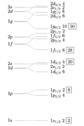
As it follows, 50 is a “magic number”, and the double-magic should be a nice spherical nuclei with filled shells. The nuclei we are interested in differ from it by (2 or 6) neutrons in the state and (6 or 10) proton holes in states. Note that those states have very different radial dependence, differing not only in orbital momentum (2 versus 4) but even in principal quantum number.
Let us calculate the corresponding wave functions. Using nuclear potential
| (20) |
with (all energies in , distances in inverse ) we calculated the corresponding wave functions, see Fig.9.
Indeed, they have very different shapes. Note, that the former one has a node, located exactly where the latter has a maximum.
The radial dependence of densities can be taken in the form
| (21) |
where the first term is a parameterization for the double-magic 50-50 nucleus. Their difference is shown in Fig.10.Note a certain excess of at large : while it is qualitatively similar to a “halo” discussed in literature, but it is not due to manybody effects but just follows from the shapes of the single-body wave functions.
Acknowledgements This work is supported by the Office of Science, U.S. Department of Energy under Contract No. DE-FG-88ER40388. I also should thank J.Jia and other organizers of BNL workshop on the subject, which prompted me to put these ideas on paper and added a talk at very short notice.
References
- Abdallah et al. (2022) Mohamed Abdallah et al. (STAR), “Search for the chiral magnetic effect with isobar collisions at =200 GeV by the STAR Collaboration at the BNL Relativistic Heavy Ion Collider,” Phys. Rev. C 105, 014901 (2022), arXiv:2109.00131 [nucl-ex] .
- Zhang and Jia (2021) Chunjian Zhang and Jiangyong Jia, “Evidence of quadrupole and octupole deformations in 96Zr+96Zr and 96Ru+96Ru collisions at ultra-relativistic energies,” (2021), arXiv:2109.01631 [nucl-th] .
- Shuryak (2000) Edward V. Shuryak, “High-energy collisions of strongly deformed nuclei: An Old idea with a new twist,” Phys. Rev. C 61, 034905 (2000), arXiv:nucl-th/9906062 .
- Escobar-Ruiz et al. (2016) M. A. Escobar-Ruiz, E. Shuryak, and A. V. Turbiner, “Quantum and thermal fluctuations in quantum mechanics and field theories from a new version of semiclassical theory,” Phys. Rev. D 93, 105039 (2016), arXiv:1601.03964 [hep-th] .
- Shuryak (1988) Edward V. Shuryak, “Toward the Quantitative Theory of the ’Instanton Liquid’ 4. Tunneling in the Double Well Potential,” Nucl. Phys. B 302, 621–644 (1988).
- Shuryak (2018) Edward Shuryak, “Lectures on nonperturbative QCD ( Nonperturbative Topological Phenomena in QCD and Related Theories),” (2018), arXiv:1812.01509 [hep-ph] .
- Escobar-Ruiz et al. (2017) M. A. Escobar-Ruiz, E. Shuryak, and A. V. Turbiner, “Fluctuations in quantum mechanics and field theories from a new version of semiclassical theory. II,” Phys. Rev. D 96, 045005 (2017), arXiv:1705.06159 [hep-th] .
- Shuryak and Turbiner (2018) E. Shuryak and A. V. Turbiner, “Transseries for the ground state density and generalized Bloch equation: Double-well potential case,” Phys. Rev. D 98, 105007 (2018), arXiv:1810.00342 [hep-th] .
- Shuryak and Torres-Rincon (2020) Edward Shuryak and Juan M. Torres-Rincon, “Baryon preclustering at the freeze-out of heavy-ion collisions and light-nuclei production,” Phys. Rev. C 101, 034914 (2020), arXiv:1910.08119 [nucl-th] .
- DeMartini and Shuryak (2021) Dallas DeMartini and Edward Shuryak, “Many-body forces and nucleon clustering near the QCD critical point,” Phys. Rev. C 104, 024908 (2021), arXiv:2010.02785 [nucl-th] .
- Gavrielov et al. (2021) N. Gavrielov, A. Leviatan, and F. Iachello, “The Zr Isotopes as a region of intertwined quantum phase transitions,” (2021), arXiv:2112.09454 [nucl-th] .