Static surface mode expansion
for the full-wave scattering from penetrable objectsC. Forestiere, G. Gravina G. Miano, G. Rubinacci are with the Department of Electrical Engineering and Information Technology, Università degli Studi di Napoli Federico II, via Claudio 21, Napoli, 80125, Italy G. Gravina is with 10th Aircraft Maintenance Department, Italian Air Force, Viale dell’Aeronautica 1, 73013 Galatina, Lecce, Italy A. Tamburrino is with Dipartimento di Ingegneria Elettrica e dell’Informazione “M. Scarano”, Università degli Studi di Cassino e del Lazio Meridionale, Via G. Di Biasio n. 43, 03043 Cassino (FR), Italy

The longitudinal static surface current modes (called in the following longitudinal static modes for brevity) are nontrivial solutions of the eigenvalue problem:

where

and $g_{0}$ is the homogeneous space static Green’s function

Apart from a multiplicative factor, the integral operator 3 gives the tangential component of the static electric field generated by a surface charge density distribution. Its spectrum has the following properties (see [25]):

1. i

   the eigenvalues $\{\gamma_{k}^{\parallel}\}$ and the corresponding eigenmodes $\{\mathbf{j}^{\parallel}_{k}\}$ depend on the shape of the object, but are independent of the object material, and of the frequency of operation;

2. ii

   the eigenvalues are real and positive;

3. iii

   the eigenmodes are orthonormal according to the scalar product 1;

The eigenvalues of a spherical surface of unit radius have the analytical expression

We now introduce a spherical coordinate system. The spherical coordinates of the point with position vector $\mathbf{r}$ are $(r,\theta,\phi)$ (with $0\leq r<\infty$, $0\leq\theta<\pi$ and $0\leq\phi<2\pi$). The basis for the three-dimensional vector space is the set $(\hat{\mathbf{r}},\hat{\boldsymbol{\theta}},\hat{\boldsymbol{\phi}})$, where $\hat{\mathbf{r}}$ is the radial unit vector, $\hat{\boldsymbol{\theta}}$ is the polar unit vector, and $\hat{\boldsymbol{\phi}}$ is the azimuthal unit vector. The eigenmodes corresponding to $\gamma_{n}^{\parallel}$ are the vector spherical harmonics $\mathbf{W}_{n}^{m}(\theta,\phi)$ where $m$ is an integer such that $-n\leq m\leq n$:

The spherical harmonic $Y_{n}^{m}\left(\theta,\phi\right)$ of degree $n$ and order $m$ is given by

where $P_{n}^{m}(\cos\theta)$ is the associated Legendre polynomial of degree $n$ and order $m$, and $C_{mn}$ is a normalization coefficient. The spherical harmonics are orthogonal. We normalize them in such a way that

where $\int(\cdot)d\Omega=\int_{0}^{\pi}d\theta\,\sin\theta\int_{0}^{2\pi}d\phi\,(\cdot)$. The normalization coefficient $C_{mn}$ is equal to

The degree $n$ also determines the multipolar order of the vector spherical harmonics (e.g. $n=1$ for a dipole, $n=2$ for a quadrupole, etc.). Thus, Eq. 5 shows that longitudinal modes associated with larger eigenvalues $\gamma^{\parallel}_{n}$ are characterized by higher multipolar order.

The transverse static surface current modes (called transverse static modes in the following for brevity) are non-trivial solutions of the eigenvalue problem:

with

Apart from a multiplicative factor, the integral operator 11 gives the static vector potential generated by a surface current distribution. Its spectrum has the following properties, that can be derived using the standard methods of eigenvalue problems, analogously to [27, 44]:

1. i

   The eigenvalues $\{\gamma_{k}^{\perp}\}$ and the modes $\{\mathbf{j}^{\perp}_{k}\}$ depend on the shape of the object, and are independent of the object material and of the frequency of operation

2. ii

   the eigenvalues are real and positive;

3. iii

   the modes $\{\mathbf{j}^{\perp}_{k}\}$ associated are orthonormal according to the scalar product 1.

The eigenvalues of a spherical surface of unit radius have the analytical expression

The modes corresponding to $\gamma_{n}^{\perp}$ are the vector spherical harmonics $\mathbf{X}_{n}^{m}(\theta,\phi)$ where $m$ is an integer such that $-n\leq m\leq n$:

The degree $n$ also determines the multipolar order of the vector spherical harmonics (e.g. $n=1$ for a dipole, $n=2$ for a quadrupole, etc.). Thus, Eq. 12 shows that transverse modes associated with smaller eigenvalues $\gamma^{\perp}_{n}$ are characterized by higher multipolar order.

Let us introduce a surface triangulation of $\partial\Omega$, with $N_{p}$ vertices, $N_{t}$ elements, and $N_{e}$ edges. We represent the static modes in term of convenient sub-domain basis functions, namely the loop and star functions [12, 45]. Specifically, any longitudinal mode $\mathbf{j}^{\parallel}_{h}$ is expanded in terms of (non-solenoidal) star basis functions $\left\{\mathbf{j}_{p}^{\star}\right\}$ with coefficients $\alpha^{\parallel\,\star}_{h,p}$. Dually, any transverse mode $\mathbf{j}^{\perp}_{h}$ is expanded in terms of (solenoidal) loop basis functions $\left\{\mathbf{j}_{q}^{\circlearrowleft}\right\}$ with coefficients $\alpha^{\perp\,\circlearrowleft}_{h,q}$:

The loop functions are divergence free, thus they correctly represent the transverse static modes. Instead, the star functions are not curl free (they are often denoted as quasi-curl [36]) thus they only approximately represent the longitudinal static modes. Both star and loop functions admit a linear representation in terms of RWG basis functions [8].

For closed surfaces with no handles, the number of linearly independent loop functions is $N_{p}-1$, while the number of linearly independent star functions is $N_{t}-1$ . Thus, the numerical auxiliary eigenvalue problem for longitudinal static modes is

where $(\text{T}_{0}^{\parallel\,{\star\star}})_{pq}=\langle\mathbf{j}_{p}^{\star},\boldsymbol{\mathcal{T}}_{0}^{\parallel}\,\mathbf{j}_{q}^{\star}\rangle$, $\left(\text{R}^{{\star\star}}\right)_{pq}=\langle\mathbf{j}_{p}^{\star},\,\mathbf{j}_{q}^{\star}\rangle,$ and $\mathbf{J}_{h}^{\star}=[\alpha^{\parallel}_{h,1},\alpha^{\parallel}_{h,2},\ldots,\alpha^{\parallel}_{h,N_{t}-1}]^{\intercal}$. The numerical auxiliary eigenvalue problem for transverse static modes is

where $\left(\text{T}^{\perp\,\circlearrowleft\circlearrowleft}\right)_{pq}=\langle\mathbf{j}_{p}^{\circlearrowleft},\boldsymbol{\mathcal{T}}_{0}^{\parallel}\,\mathbf{j}_{q}^{\circlearrowleft}\rangle,\quad\left(\text{R}^{{\circlearrowleft\circlearrowleft}}\right)_{pq}=\langle\mathbf{j}_{p}^{\circlearrowleft},\,\mathbf{j}_{q}^{\circlearrowleft}\rangle$, and $\mathbf{J}_{h}^{\circlearrowleft}=[\alpha^{\perp}_{h,1},\alpha^{\perp}_{h,2},\ldots,\alpha^{\perp}_{h,N_{p}-1}]^{\intercal}$.

Since the loop and star functions are not orthogonal, the matrices $\text{R}^{{\star\star}}$ and $\text{R}^{{\circlearrowleft\circlearrowleft}}$ are not identity matrices, thus Eqs. 15 and 16 are generalized eigenvalue problems. The involved matrices are real, symmetric, and positive definite. Thus, efficient numerical algorithms for the eigenvalue calculation do apply, such as the Cholesky factorization [46]. Moreover, the matrices properties also determine the orthogonality, at the discrete level, of any pair of longitudinal modes, and any pair of transverse modes. The numerical integration of shape functions times the Green’s functions or its gradient are evaluated using the techniques introduced by Graglia [47].

Aiming at the solution of the PMCWHT equation 17, we represent the equivalent electric and magnetic surface currents in terms of the transverse static modes $\{\mathbf{j}^{\perp}_{p}\}_{p=1\ldots\text{N}^{\perp}}$ associated with the first $\text{N}^{\perp}$ eigenvalues $\gamma_{p}^{\perp}$ (sorted in descending order), and in terms of the longitudinal static modes $\{\mathbf{j}^{\parallel}_{q}\}_{q=1\ldots\text{N}^{\parallel}}$ associated with the first $\text{N}^{\parallel}$ eigenvalues $\gamma_{q}^{\parallel}$ (sorted in ascending order), namely

The choice of sorting the longitudinal eigenvalues accordingly to an ascending order and the transverse eigenvalues accordingly to a descending order guarantees that low-index eigenvalues are associated with modes of low-order multipolar order (dipole, quadrupole, octupole …).

Therefore, we define the unknown block vectors

with $\boldsymbol{\alpha}^{a}=\left[\alpha_{1}^{a},\alpha_{2}^{a},\ldots,\alpha_{\text{N}^{a}}^{a}\right]^{\intercal}$ and with $\boldsymbol{\beta}^{a}=\left[\beta_{1}^{a},\beta_{2}^{a},\ldots,\beta_{\text{N}^{a}}^{a}\right]^{\intercal}$ and $a=\parallel,\perp$

We find the finite dimensional approximation of the PMCHWT problem by substituting Eq. 23 in Eq. 17 and by projecting along the same set of modes, accordingly to a Galerkin projection scheme:

where

and

with $a,b=\parallel,\perp$. The finite dimensional system has $2(\text{N}^{\parallel}+\text{N}^{\perp})$ degrees of freedom.

We now decompose the Green’s function as the sum of the static Green’s function $g_{0}$ and a regular difference term $g_{d\pm}$:

where

In the past, the splitting of the Green’s function into its static component and a difference term has been used to introduce well-conditioned and accurate scheme for the low-frequency analysis of PEC targets with the MFIE [48]. By applying this decomposition to the operators $\boldsymbol{\mathcal{T}}_{\pm}$ and $\boldsymbol{\mathcal{K}}_{\pm}$, defined in 21a and 21, we obtain:

where $\boldsymbol{\mathcal{T}}_{0}^{\parallel}$ and $\boldsymbol{\mathcal{T}}_{0}^{\perp}$ are the static operators defined in Eqs. 3 and 11, and

The above decomposition considerably simplifies the calculation of the finite dimensional operators $\text{T}_{\pm}^{a\,b}$ with $a,b=\parallel,\perp$, which are obtained by projecting the operator $\boldsymbol{\mathcal{T}}_{\pm}$ along the longitudinal and transverse static modes because $\{\mathbf{j}^{\parallel}_{k}\}$ and $\{\mathbf{j}^{\perp}_{k}\}$ diagonalize the static operators $\boldsymbol{\mathcal{T}}_{0}^{\perp}$ and $\boldsymbol{\mathcal{T}}_{0}^{\parallel}$:

where $\delta_{p,q}$ is the Kronecker delta. We point out that the numerical computation of the terms $\langle\mathbf{j}^{\parallel}_{p},\boldsymbol{\mathcal{T}}_{d\pm}\,\mathbf{j}^{\perp}_{q}\rangle$ is straightforward, since their kernels are regular functions. These terms are the only ones depending on the operating frequency. The decomposition of the Green’s function into the sum of a static term and of a regular difference term relieves us from the task of computing almost all the integrals with (integrable) singularity, which usually results in longer computational time compared to their regular counterpart. There are however two exceptions: $\langle\mathbf{j}^{\parallel}_{p},\boldsymbol{\mathcal{T}}_{0}^{\perp}\,\mathbf{j}^{\parallel}_{q}\rangle$ and $\langle\mathbf{j}^{a}_{p},\boldsymbol{\mathcal{K}}_{0}^{\perp}\,\mathbf{j}_{q}^{b}\rangle$, $\forall a,b\in\perp,\parallel$. These terms are frequency-independent, thus when the calculation of the scattering response of an object for multiple frequencies of the exciting field is required, they can be conveniently precalculated and stored away, while only the regular terms must be calculated at any frequencies.

Surface integral formulations may suffer from ill-conditioning due to low frequency breakdown. The low frequency breakdown phenomenon manifests when the operating wavelength is much larger than the dimension of the object [49], and originates from the different frequency-scaling of the terms associated with the vector and the scalar potentials. This is a common scenario which may be encountered in several applications, including metamaterials and electromagnetic bandgap (EBG) structures, or in the analysis of interconnects and packaging. This problem has been addressed by using quasi-Helmholtz decompositions, such as loop/star [49, 45, 50], loop-tree [13, 51], or null-pinv [52] decomposition, followed by a basis rearrangement [53, 54]. It is also worth to point out that some formulations are immune from this problem, such as the N-Müller formulation [55], or the formulation obtained by augmenting the traditional EFIE by including charge as extra unknown [56, 57].

In this section, we summarize the behaviour of the PMCHWT at very low frequencies. In this limit, the frequency dependence of the elements of the matrix Z follows different scaling laws, which are easily determined by following [54, 58]

where ${\Gamma}^{\perp}$ and ${\Gamma}^{\parallel}$ are diagonal matrices, ${\Gamma}^{\perp}=\text{diag}\left\{\gamma^{\perp}_{1},\gamma^{\perp}_{2},\ldots,\gamma^{\perp}_{\text{N}^{\perp}}\right\},$ ${\Gamma}^{\parallel}=\text{diag}\left\{\gamma^{\parallel}_{1},\gamma^{\parallel}_{2},\ldots,\gamma^{\parallel}_{\text{N}^{\parallel}}\right\},$ and

Thus, by using Eqs. 39 and 40 it easy to prove that, in the static limit, the discrete matrix Z approaches the matrix $\text{Z}_{0}$ which exhibits the following frequency dependence:

The excitation vector associated with a plane wave exhibits the following dependencies [54]:

Following [54], we introduce the rearrangement and scaling of the basis

where ${D}_{1}=\text{diag}\left\{k_{-}^{-1}\text{I}_{\text{N}^{\perp}},\text{I}_{\text{N}^{\parallel}},k_{-}^{-1}\text{I}_{\text{N}^{\perp}},\text{I}_{\text{N}^{\parallel}}\right\}$, ${D}_{2}=\text{diag}\left\{\text{I}_{\text{N}^{\perp}},ik_{-}\text{I}_{\text{N}^{\parallel}},\text{I}_{\text{N}^{\perp}},ik_{-}\text{I}_{\text{N}^{\parallel}}\right\},$ $\text{I}_{\text{N}^{\perp}}$ is the the $\text{N}^{\perp}\times\text{N}^{\perp}$ identity matrix, and $\text{I}_{\text{N}^{\parallel}}$ is the $\text{N}^{\parallel}\times\text{N}^{\parallel}$ identity matrix. After the above rearrangement the matrix $\tilde{\text{Z}}$ is well-behaved.

We first consider the scattering from a sphere. This problem has an analytical solution [59, 17].

Figure 1 shows the convergence of the eigenvalues $\{\gamma_{k}^{\parallel}\}$ and $\{\gamma_{k}^{\perp}\}$ toward their analytical counterpart, given by Eqs. 5 and 12, as a function of the triangular mesh density. From now on, we consider the static basis calculated using a triangular mesh with $N_{p}=1000$ nodes and $N_{t}=1996$ triangles. The first 8 longitudinal modes are shown in Fig. 2, the first 8 transverse modes are shown in Fig. 3.

In the discrete problem, the orthogonality between any pair of longitudinal modes and between any pair of transverse modes is always guaranteed, because the matrices $\text{T}^{\circlearrowleft\circlearrowleft}$ and $\text{T}^{\star\star}$ are real and symmetric. This property is indeed verified at the numerical level with machine precision. Instead, even if we expect that the mutual product between a transverse and a longitudinal static mode to be vanishing, this fact is only approximately verified, since the sub-domain basis functions used to represent the longitudinal modes, namely the “star” functions, are not rigorously curl-free [50]. Thus, it is worth calculating the “mutual” Gram matrix G, whose occurrences are defined as $g_{hk}=\langle\mathbf{j}_{h}^{\perp},\mathbf{\bf j}_{k}^{\parallel}\rangle$. The maximum occurrence of the mutual Gram matrix is 0.024 for a sphere with the considered surface mesh, assuming $\|\mathbf{j}_{h}^{\parallel}\|=\|\mathbf{j}_{h}^{\perp}\|=1$, $\forall h$.

We now consider a non-canonical shape, namely a three-dimensional rod. We model this shape as a superellipsoid, whose boundary has the implicit equation $\left({x}/{a}\right)^{r}+\left({y}/{b}\right)^{r}+\left({z}/{a}\right)^{r}=1,$ with $b=0.5a$, $c=0.25a$, and $r=6$. We used the public domain code developed by Per-Olof Persson and Gilbert Strang [62] to generate a surface mesh with $1000$ nodes and $1996$ triangular elements. The first 8 longitudinal and 8 transverse static modes are shown in Fig. 12 and 13, respectively.

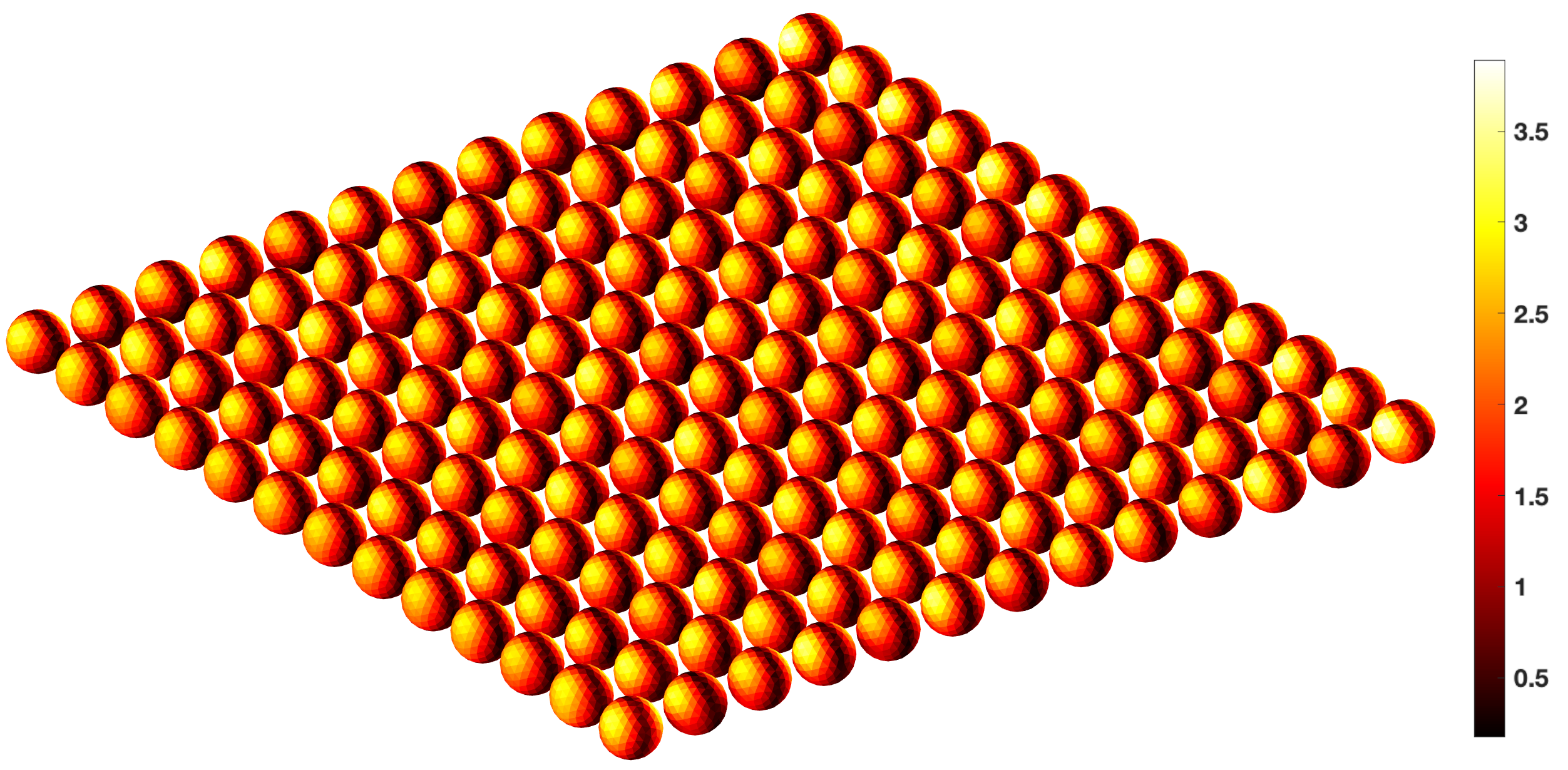
The static mode basis finds its natural application in the numerical solution of multiple scattering problems, where an array, whose dimension can be much larger than the incident wavelength, is made of $n$ objects with identical shape but with different orientation and size.

We support the above statement through several examples. Specifically, we consider a finite-size periodic array of $n$ spheres, of radius $R=100nm$, which are placed at the nodes of a $\sqrt{n}\times\sqrt{n}$ square grid of pitch $250$nm. The values of pitch and radius also fix the edge-edge interparticle separation to $50$ nm. The geometry of a $13\times 13$ array of $169$ spheres is shown in Fig. 18. The array is excited by a plane wave, linearly polarized in the plane of the array, along one of the two axis, and propagating in the direction orthogonal to the array’s plane with wavelength $\lambda=600$nm. Each sphere is described by a surface mesh having $200$ nodes and $396$ triangles and $594$ edges, which corresponds to a maximum edge length of the mesh’s triangles $\approx\lambda/17$. A loop/star description leads to $1188\,n$ unknowns. Instead, we considered $\text{N}^{\parallel}$ longitudinal and $\text{N}^{\perp}=10$ transverse modes to describe the electric and magnetic surface currents on each nanoparticle, which correspond to $40\,n$ unknowns ( a reduction of more than one order of magnitude).

In Fig. 19, we show the cpu time (in seconds) of the different stages of the numerical solution of the scattering problem from the finite-size periodic array of spheres, as a function of the number $n$ of spheres ($n=1,4,9,16,\ldots,169$). The FORTRAN code runs on a single cpu. The total computational time is always dominated by the compression time, which scales as $\propto n^{2}$. The assembly time, which also scales as $\propto n^{2}$, gives an important contribution to the total execution time. The time required for the computation of the static modes of the isolated sphere, which are used as basis, is negligible and it does not depend on the array’s size. The inversion time, which scales as $\propto n^{3}$, is negligible if compared with the compression time, as in our case, if the dimensions of the arrays do not exceed a given number of particles ($n_{th}$). The value of $n_{th}$ can be estimated extrapolating the the curves in Fig. 19, and it is $n_{th}\approx 80k$ particles.

In Fig. 20 we compare the total cpu-time required for the solution of the PMCHWT solution using the static modes basis against the corresponding time required to obtain the loop/star solution, as a function of $n$. For $n>4$, the static mode solution becomes advantageous, and the speed up further increases as $n$ increases. In Tab. I, we also compare for $n\leq 25$ the error made by the static mode solution compared to the loop/star reference: it is always less then $4\%$ for both the scattering efficiency and the currents.

To obtain information on the scaling laws, we fit the total computational time of the solution of the PMCHWT in terms of the static basis using the curve $t=3n^{2}$, and in terms of the loop/star solution using the curve $t=0.92n^{3}$. The ratio is $0.3n$. Thus, for a $5\times 5$ array, the cpu-time required to obtain the loop/star solution is $7.5$ time larger than the cpu-time required for the static mode solution. For $n=169$ we extrapolate that the static mode solution is $50\times$ faster, but it was not possible to verify it experimentally, since the time expected to compute the loop/star solution was prohibitive.

In Fig. 18, we plot the magnitude of the total electric field on the surface of each sphere of the $n=169$ sphere array. For this case $n=169$, we consider $520$ static modes. The corresponding loop/star description would require $200k$ unknowns.

References

- [1] R. E. Collin, Antennas and Radiowave Propagation. McGraw-Hill College, 1985. [Online]. Available: https://books.google.it/books/about/Antennas_and_Radiowave_Propagation.html?id=YHepAAAACAAJ&redir_esc=y
- [2] N. Yu and F. Capasso, “Flat optics with designer metasurfaces,” Nature Materials, vol. 13, no. 2, pp. 139–150, Feb. 2014, bandiera_abtest: a Cg_type: Nature Research Journals Number: 2 Primary_atype: Reviews Publisher: Nature Publishing Group Subject_term: Metamaterials Subject_term_id: metamaterials. [Online]. Available: https://www.nature.com/articles/nmat3839
- [3] M. Khorasaninejad, F. Aieta, P. Kanhaiya, M. A. Kats, P. Genevet, D. Rousso, and F. Capasso, “Achromatic Metasurface Lens at Telecommunication Wavelengths,” Nano Letters, vol. 15, no. 8, pp. 5358–5362, Aug. 2015. [Online]. Available: https://doi.org/10.1021/acs.nanolett.5b01727
- [4] W. C. Chew, J.-M. Jin, E. Michielssen, and J. Song, Eds., Fast and Efficient Algorithms in Computational Electromagnetics. Boston: Artech House, Jul. 2000.
- [5] O. M. Bucci and G. D. Massa, “Use of characteristic modes in multiple-scattering problems,” Journal of Physics D: Applied Physics, vol. 28, no. 11, p. 2235, Nov. 1995. [Online]. Available: https://iopscience.iop.org/article/10.1088/0022-3727/28/11/003/meta
- [6] G. Angiulli, G. Amendola, and G. D. Massa, “Characteristic Modes in Multiple Scattering by Conducting Cylinders of Arbitrary Shape,” Electromagnetics, vol. 18, no. 6, pp. 593–612, Nov. 1998, publisher: Taylor & Francis _eprint: https://doi.org/10.1080/02726349808908615. [Online]. Available: https://doi.org/10.1080/02726349808908615
- [7] A. Doicu, T. Wriedt, and Y. A. Eremin, Light Scattering by Systems of Particles: Null-Field Method with Discrete Sources: Theory and Programs, ser. Springer Series in Optical Sciences. Berlin Heidelberg: Springer-Verlag, 2006. [Online]. Available: https://www.springer.com/gp/book/9783540336969
- [8] S. Rao, D. Wilton, and A. Glisson, “Electromagnetic scattering by surfaces of arbitrary shape,” IEEE Transactions on Antennas and Propagation, vol. 30, no. 3, pp. 409–418, May 1982, conference Name: IEEE Transactions on Antennas and Propagation.
- [9] A. Bossavit, Computational electromagnetism: variational formulations, complementarity, edge elements. Academic Press, 1998.
- [10] R. Albanese and G. Rubinacci, “Integral formulation for 3D eddy-current computation using edge elements,” IEE Proceedings A (Physical Science, Measurement and Instrumentation, Management and Education, Reviews), vol. 135, no. 7, pp. 457–462, 1988.
- [11] G. Rubinacci and A. Tamburrino, “A broadband volume integral formulation based on edge-elements for full-wave analysis of lossy interconnects,” IEEE transactions on antennas and propagation, vol. 54, no. 10, pp. 2977–2989, 2006.
- [12] D. Wilton, J. Lim, and S. Rao, “A novel technique to calculate the electromagnetic scattering by surfaces of arbitrary shape,” URSI Radio Science Meeting, p. 322, 1993.
- [13] W.-L. Wu, A. W. Glisson, and D. Kajfez, “A study of two numerical solution procedures for the electric field integral equation at low frequency,” Applied Computational Electromagnetics Society Journal, vol. 10, no. 3, pp. 69–80, 1995.
- [14] L. Trintinalia and H. Ling, “First Order Triangular Patch Basis Functions for Electromagnetic Scattering Analysis,” Journal of Electromagnetic Waves and Applications, vol. 15, no. 11, pp. 1521–1537, Jan. 2001, publisher: Taylor & Francis _eprint: https://doi.org/10.1163/156939301X00085. [Online]. Available: https://doi.org/10.1163/156939301X00085
- [15] A. Buffa and S. H. Christiansen, “A Dual Finite Element Complex on the Barycentric Refinement,” Mathematics of Computation, vol. 76, no. 260, pp. 1743–1769, 2007, publisher: American Mathematical Society. [Online]. Available: https://www.jstor.org/stable/40234460
- [16] R. Graglia, D. Wilton, and A. Peterson, “Higher order interpolatory vector bases for computational electromagnetics,” IEEE Transactions on Antennas and Propagation, vol. 45, no. 3, pp. 329–342, Mar. 1997, conference Name: IEEE Transactions on Antennas and Propagation.
- [17] C. F. Bohren and D. R. Huffman, Absorption and Scattering of Light by Small Particles. Wiley, 1998.
- [18] L.-W. Li, X.-K. Kang, and M.-S. Leong, Spheroidal Wave Functions in Electromagnetic Theory. John Wiley & Sons, Apr. 2004.
- [19] R. Garbacz, “Modal expansions for resonance scattering phenomena,” Proceedings of the IEEE, vol. 53, no. 8, pp. 856–864, 1965.
- [20] Y. Chang and R. Harrington, “A surface formulation for characteristic modes of material bodies,” IEEE Transactions on Antennas and Propagation, vol. 25, no. 6, pp. 789–795, Nov. 1977, conference Name: IEEE Transactions on Antennas and Propagation.
- [21] R. Harrington, J. Mautz, and Yu Chang, “Characteristic modes for dielectric and magnetic bodies,” IEEE Transactions on Antennas and Propagation, vol. 20, no. 2, pp. 194–198, Mar. 1972.
- [22] Y. Chen and C.-F. Wang, Characteristic Modes: Theory and Applications in Antenna Engineering. John Wiley & Sons, Jun. 2015, google-Books-ID: suobBgAAQBAJ.
- [23] M. Faenzi, G. Minatti, D. González-Ovejero, F. Caminita, E. Martini, C. Della Giovampaola, and S. Maci, “Metasurface Antennas: New Models, Applications and Realizations,” Scientific Reports, vol. 9, no. 1, p. 10178, Jul. 2019. [Online]. Available: https://www.nature.com/articles/s41598-019-46522-z
- [24] C. Forestiere, G. Gravina, G. Miano, M. Pascale, and R. Tricarico, “Electromagnetic modes and resonances of two-dimensional bodies,” Physical Review B, vol. 99, no. 15, p. 155423, Apr. 2019, publisher: American Physical Society. [Online]. Available: https://link.aps.org/doi/10.1103/PhysRevB.99.155423
- [25] I. D. Mayergoyz, D. R. Fredkin, and Z. Zhang, “Electrostatic (plasmon) resonances in nanoparticles,” Phys. Rev. B, vol. 72, no. 15, p. 155412, Oct. 2005. [Online]. Available: https://link.aps.org/doi/10.1103/PhysRevB.72.155412
- [26] G. Miano, G. Rubinacci, and A. Tamburrino, “Numerical Modeling for the Analysis of Plasmon Oscillations in Metallic Nanoparticles,” IEEE Transactions on Antennas and Propagation, vol. 58, no. 9, pp. 2920–2933, 2010.
- [27] C. Forestiere, G. Miano, G. Rubinacci, M. Pascale, A. Tamburrino, R. Tricarico, and S. Ventre, “Magnetoquasistatic resonances of small dielectric objects,” Phys. Rev. Research, vol. 2, no. 1, p. 013158, Feb. 2020. [Online]. Available: https://link.aps.org/doi/10.1103/PhysRevResearch.2.013158
- [28] C. Forestiere, G. Miano, M. Pascale, and R. Tricarico, “Quantum theory of radiative decay rate and frequency shift of surface plasmon modes,” Physical Review A, vol. 102, no. 4, p. 043704, Oct. 2020, publisher: American Physical Society. [Online]. Available: https://link.aps.org/doi/10.1103/PhysRevA.102.043704
- [29] C. Forestiere and G. Miano, “Operative approach to quantum electrodynamics in dispersive dielectric objects based on a polarization-mode expansion,” Physical Review A, vol. 106, no. 3, p. 033701, Sep. 2022, publisher: American Physical Society. [Online]. Available: https://link.aps.org/doi/10.1103/PhysRevA.106.033701
- [30] C. Forestiere, G. Miano, and G. Rubinacci, “Resonance frequency and radiative Q-factor of plasmonic and dieletric modes of small objects,” Phys. Rev. Research, vol. 2, no. 4, p. 043176, Nov. 2020. [Online]. Available: https://link.aps.org/doi/10.1103/PhysRevResearch.2.043176
- [31] C. Forestiere and G. Miano, “Time-domain formulation of electromagnetic scattering based on a polarization-mode expansion and the principle of least action,” Physical Review A, vol. 104, no. 1, p. 013512, Jul. 2021, publisher: American Physical Society. [Online]. Available: https://link.aps.org/doi/10.1103/PhysRevA.104.013512
- [32] E. Suter and J. R. Mosig, “A subdomain multilevel approach for the efficient MoM analysis of large planar antennas,” Microwave and Optical Technology Letters, vol. 26, no. 4, pp. 270–277, 2000
- [33] V. V. S. Prakash and R. Mittra, “Characteristic basis function method: A new technique for efficient solution of method of moments matrix equations,” Microwave and Optical Technology Letters, vol. 36, no. 2, pp. 95–100, 2003, _eprint: https://onlinelibrary.wiley.com/doi/pdf/10.1002/mop.10685. [Online]. Available: https://onlinelibrary.wiley.com/doi/abs/10.1002/mop.10685
- [34] L. Matekovits, V. A. Laza, and G. Vecchi, “Analysis of Large Complex Structures With the Synthetic-Functions Approach,” IEEE Transactions on Antennas and Propagation, vol. 55, no. 9, pp. 2509–2521, Sep. 2007, conference Name: IEEE Transactions on Antennas and Propagation.
- [35] A. Freni, P. De Vita, P. Pirinoli, L. Matekovits, and G. Vecchi, “Fast-Factorization Acceleration of MoM Compressive Domain-Decomposition,” IEEE Transactions on Antennas and Propagation, vol. 59, no. 12, pp. 4588–4599, Dec. 2011, conference Name: IEEE Transactions on Antennas and Propagation.
- [36] G. Vecchi, L. Matekovits, P. Pirinoli, and M. Orefice, “Hybrid spectral-spatial method for the analysis of printed antennas,” Radio Science, vol. 31, no. 5, pp. 1263–1270, Sep. 1996, conference Name: Radio Science.
- [37] ——, “A numerical regularization of the EFIE for three-dimensional planar structures in layered media (invited article),” International Journal of Microwave and Millimeter-Wave Computer-Aided Engineering, vol. 7, no. 6, pp. 410–431, 1997
- [38] T.-K. Wu and L. L. Tsai, “Scattering from arbitrarily-shaped lossy dielectric bodies of revolution,” Radio Science, vol. 12, no. 5, pp. 709–718, 1977
- [39] A. J. Poggio and E. K. Miller, “CHAPTER 4 - Integral Equation Solutions of Three-dimensional Scattering Problems,” in Computer Techniques for Electromagnetics, ser. International Series of Monographs in Electrical Engineering, R. Mittra, Ed. Pergamon, Jan. 1973, pp. 159–264.
- [40] R. F. Harrington, Field computation by moment methods. Wiley-IEEE Press, 1993.
- [41] P. Monk and D. o. M. S. P. M. PH, Finite Element Methods for Maxwell’s Equations. Clarendon Press, Apr. 2003.
- [42] R. Scharstein, “Helmholtz decomposition of surface electric current in electromagnetic scattering problems,” in [1991 Proceedings] The Twenty-Third Southeastern Symposium on System Theory, Mar. 1991, pp. 424–426, iSSN: 0094-2898.
- [43] N. V. Nair and B. Shanker, “Generalized Method of Moments: A Novel Discretization Technique for Integral Equations,” IEEE Transactions on Antennas and Propagation, vol. 59, no. 6, pp. 2280–2293, Jun. 2011, conference Name: IEEE Transactions on Antennas and Propagation.
- [44] A. Tamburrino, G. Piscitelli, and Z. Zhou, “The monotonicity principle for magnetic induction tomography,” Inverse Problems, vol. 37, no. 9, p. 095003, Aug. 2021.
- [45] M. Burton and S. Kashyap, “A study of a recent, moment-method algorithm that is accurate to very low frequencies,” Applied Computational Electromagnetics Society Journal, vol. 10, pp. 58–68, 1995, publisher: APPLIED COMPUTATIONAL ELECTROMAGNETICS SOCIETY INC.
- [46] H. Golub and C. F. V. Loan, Matrix Computations. Baltimore, MD: Johns Hopkins University Press, 1983.
- [47] R. Graglia, “On the numerical integration of the linear shape functions times the 3-D Green’s function or its gradient on a plane triangle,” Antennas and Propagation, IEEE Transactions on, vol. 41, no. 10, pp. 1448 –1455, Oct. 1993.
- [48] E. Ubeda and J. M. Rius, “Divergence-conforming discretization of second-kind integral equations for the RCS computation in the Rayleigh frequency region,” Radio Science, vol. 46, no. 05, pp. 1–10, Oct. 2011, conference Name: Radio Science.
- [49] D. R. Wilton and A. W. Glisson, “On improving the electric field inte-gral equation at low frequencies,” Los Angeles, CA, Jun. 1981, pp. 22–24.
- [50] G. Vecchi, “Loop-star decomposition of basis functions in the discretization of the EFIE,” IEEE Transactions on Antennas and Propagation, vol. 47, no. 2, pp. 339–346, Feb. 1999, conference Name: IEEE Transactions on Antennas and Propagation.
- [51] F. P. Andriulli, “Loop-Star and Loop-Tree Decompositions: Analysis and Efficient Algorithms,” IEEE Transactions on Antennas and Propagation, vol. 60, no. 5, pp. 2347–2356, May 2012, conference Name: IEEE Transactions on Antennas and Propagation.
- [52] G. Miano and F. Villone, “A surface integral formulation of Maxwell equations for topologically complex conducting domains,” IEEE Transactions on Antennas and Propagation, vol. 53, no. 12, pp. 4001–4014, Dec. 2005, conference Name: IEEE Transactions on Antennas and Propagation.
- [53] J.-S. Zhao and W. C. Chew, “Integral equation solution of Maxwell’s equations from zero frequency to microwave frequencies,” IEEE Transactions on Antennas and Propagation, vol. 48, no. 10, pp. 1635–1645, Oct. 2000, conference Name: IEEE Transactions on Antennas and Propagation.
- [54] S. Chen, W. C. Chew, J. Song, and J.-S. Zhao, “Analysis of low frequency scattering from penetrable scatterers,” IEEE Transactions on Geoscience and Remote Sensing, vol. 39, no. 4, pp. 726–735, Apr. 2001, conference Name: IEEE Transactions on Geoscience and Remote Sensing.
- [55] P. Ylä-Oijala, H. Wallén, D. C. Tzarouchis, and A. Sihvola, “Surface Integral Equation-Based Characteristic Mode Formulation for Penetrable Bodies,” IEEE Transactions on Antennas and Propagation, vol. 66, no. 7, pp. 3532–3539, Jul. 2018, conference Name: IEEE Transactions on Antennas and Propagation.
- [56] M. Taskinen and P. Yla-Oijala, “Current and charge Integral equation formulation,” IEEE Transactions on Antennas and Propagation, vol. 54, no. 1, pp. 58–67, Jan. 2006, conference Name: IEEE Transactions on Antennas and Propagation.
- [57] Z. G. Qian and W. C. Chew, “An augmented electric field integral equation for high-speed interconnect analysis,” Microwave and Optical Technology Letters, vol. 50, no. 10, pp. 2658–2662, 2008, _eprint: https://onlinelibrary.wiley.com/doi/pdf/10.1002/mop.23736. [Online]. Available: https://onlinelibrary.wiley.com/doi/abs/10.1002/mop.23736
- [58] C. Forestiere, G. Miano, G. Rubinacci, A. Tamburrino, L. Udpa, and S. Ventre, “A Frequency Stable Volume Integral Equation Method for Anisotropic Scatterers,” IEEE Transactions on Antennas and Propagation, vol. 65, no. 3, pp. 1224–1235, Mar. 2017.
- [59] G. Mie, “Beiträge zur Optik trüber Medien, speziell kolloidaler Metallösungen,” Annalen der physik, vol. 330, no. 3, pp. 377–445, 1908.
- [60] P. B. Johnson and R. W. Christy, “Optical Constants of the Noble Metals,” Phys. Rev. B, vol. 6, no. 12, pp. 4370–4379, Dec. 1972. [Online]. Available: https://link.aps.org/doi/10.1103/PhysRevB.6.4370
- [61] J. A. Schuller, E. S. Barnard, W. Cai, Y. C. Jun, J. S. White, and M. L. Brongersma, “Plasmonics for extreme light concentration and manipulation,” Nat. Mater., vol. 9, pp. 193–204, 2010.
- [62] P.-O. Persson and G. Strang, “A Simple Mesh Generator in Matlab,” SIAM Review, vol. 46, no. 2, pp. 329–345, 2004, publisher: Society for Industrial and Applied Mathematics. [Online]. Available: https://www.jstor.org/stable/20453511
- [63] A. Nosich, “The method of analytical regularization in wave-scattering and eigenvalue problems: foundations and review of solutions,” IEEE Antennas and Propagation Magazine, vol. 41, no. 3, pp. 34–49, Jun. 1999, conference Name: IEEE Antennas and Propagation Magazine.