Evolved interactions stabilize many coexisting phases in multicomponent liquids
Abstract
Phase separation has emerged as an essential concept for the spatial organization inside biological cells. However, despite the clear relevance to virtually all physiological functions, we understand surprisingly little about what phases form in a system of many interacting components, like in cells. Here, we introduce a new numerical method based on physical relaxation dynamics to study the coexisting phases in such systems. We use our approach to optimize interactions between components, similar to how evolution might have optimized the interactions of proteins. These evolved interactions robustly lead to a defined number of phases, despite substantial uncertainties in the initial composition, while random or designed interactions perform much worse. Moreover, the optimized interactions are robust to perturbations and they allow fast adaption to new target phase counts. We thus show that genetically encoded interactions of proteins provide versatile control of phase behavior. The phases forming in our system are also a concrete example of a robust emergent property that does not rely on fine-tuning the parameters of individual constituents.
Biological cells are incredibly complex and consist of thousands of different biomolecules that move and react rapidly. Yet, cells display robust behavior, partly because they separate molecules into distinct compartments. One important class of compartments are biomolecular condensates, which have now been identified in eukaryotes Brangwynne et al. 2009; Feric et al. 2016; Banani et al. 2017, procaryotes Azaldegui et al. 2020; Cohan and Pappu 2020; Greening and Lithgow 2020, and plants Emenecker et al. 2021; Kim et al. 2021. In all systems, multiple different condensates coexist and some condensates, like the nucleolus Lafontaine et al. 2020 and nuclear speckles Fei et al. 2017, even possess sub-compartments. The collective organization of biomolecules into condensates is explained by phase separation Fritsch et al. 2021, which is a physical mechanism where a gain in enthalpic interactions offsets the entropy loss when molecules are confined. Since all proteins interact weakly by various mechanisms Dignon et al. 2020, phase separation is widely expected in the proteome Hardenberg et al. 2020 and transcriptome Adekunle and Hubstenberger 2020. However, it is still mysterious how cells regulate phase separation.
Biomolecular condensates need to form robustly, despite internal and external uncertainties that cells cannot control. Having the right condensates, in the right situation, at the right time is crucial since condensates participate in almost all cellular processes Lyon et al. 2020, they affect the fitness of prokaryotes Jin et al. 2021, and malfunctioning is implicated in many diseases Alberti and Dormann 2019. It is particularly mysterious how cells reliably form many different kinds of condensates in a common cytosol, despite copy number fluctuations of all components. Are the interactions between components tuned such that the right condensates form reliably? It is conceivable that multiple driving forces of phase separation Dignon et al. 2020 have been adjusted over evolutionary time scales. Indeed, theoretical studies Saar et al. 2021; Choi et al. 2020, numerical simulations Harmon et al. 2017; Lin et al. 2018, and in vitro experiments Schuster et al. 2020; Bremer et al. 2021 demonstrated that small modifications of the sequence of a protein can have profound impact on its phase separation. However, it is not clear whether these results on single components can be transferred to multicomponent mixtures.
While the theoretical basis of phase separation is well-understood Hyman et al. 2014; Brangwynne et al. 2015; Berry et al. 2018; Weber et al. 2019, even predicting equilibrium states is challenging in multicomponent mixtures. This is due to enormous variability in heterotypic interactions, which leads to complex phase diagrams Riback et al. 2020. We can now construct complete phase diagrams for up to components Mao et al. 2018 and predict the associated phase morphology Mao et al. 2020. This showed that the number of coexisting phases typically depends on the overall composition of the system, but it is unclear how this phase count depends on the component count and the specific interaction matrix. Answering this question is critical, since typical biological condensates consist of many components Leung et al. 2003; Updike and Strome 2009; Riback et al. 2020; Currie and Rosen 2021 and the scaffold-client picture Banani et al. 2016, where a single scaffold component dominates the phase behavior, might not always apply. State-of-the art numerical techniques can simulate mixtures of up to components Zhou and Xie 2021; Shrinivas and Brenner 2021, but these techniques are often too costly to truly explore the space of possible interactions. Random matrix theory provides an alternative approach to investigate the stability of mixtures comprising very many components whose interactions are chosen from a random distribution Sear and Cuesta 2003; Jacobs and Frenkel 2013; Jacobs and Frenkel 2017; Shrinivas and Brenner 2021; Jacobs 2021. While these studies demonstrated that phase separation is overwhelmingly likely in such systems, it is unclear how well random interactions capture real proteins, which have evolved for millions of generations. In fact, it is unclear what properties of interacting proteins need to be conserved during evolution for a robust phase separation behavior.
Results
We here present a novel approach to analyze multiphase equilibrium states of multicomponent liquids, which is based on relaxation dynamics. We then use this model to investigate how components need to interact such that a given number of phases forms reliably.
A simplified physical model reveals equilibrium states
We consider an isothermal, incompressible liquid comprised of different components and an inert solvent. In equilibrium, such a system can in principle form liquid phases Gibbs 1876, which are homogeneous regions with distinct composition. However, in typical realistic systems fewer phases form since some components might be miscible. To reveal how the number of phases formed depends on the interactions of the components, we consider the general case of coexisting phases with volumes for . Since phases are homogeneous, their composition is fully described by the particle counts for each component or the associated volume fractions , where we consider equal molecular volumes for simplicity. Note that the fraction of the inert solvent, , is not an independent variable. Multiple phases can coexist when the associated free energy is minimal, where is the free energy density that depends on the local composition. We here consider regular solution theory, Flory 1942
| (1) |
where is the thermal energy scale and the first two terms capture the entropic contributions of the solvent and all other components, respectively. Conversely, the last term quantifies the enthalpic interaction between all components. The elements of the interaction matrix can for instance be derived from the interaction energies between components and on a lattice, , where is the lattice coordination number Cahn and Hilliard 1958; Mao et al. 2018. This implies that the diagonal entries vanish, , while the off-diagonal entries capture the relevant balance between heterotypic and homotypic interactions; see Fig. 1A. Note that effective repulsion () can originate not only from heterotypic repulsion (), but also from homotypic attraction that outweighs the heterotypic interaction ().
The multicomponent liquid reaches equilibrium when is minimal, implying that the chemical potentials and the pressures are equal between all phases Weber et al. 2019. We express these quantities in non-dimensional form, and , for each phase ,
| (2a) | ||||
| (2b) | ||||
The equilibrium conditions for the system then read
| (3a) | ||||
| (3b) | ||||
for , which are and non-linear equations, respectively. Additionally, there are equations for the conservation of particles, , and an equation for volume conservation, . Taken together, these equations can in principle be solved for the volumes and particle counts , although this is generally challenging Mao et al. 2018.

The equilibrium conditions (3) describe the local coexistence of phases of potentially different composition . Since these conditions only involve the intensive quantities , coexisting volume fractions can be determined without specifying the extensive volumes , similar to the Maxwell construction in a binary system Weber et al. 2019. In multicomponent systems, such equilibrium points correspond to the stationary state of a simple dynamical system,
| (4) |
where is a non-dimensional time and the interaction matrix is the only parameter; see Eq. (2). Clearly, Eq. (4) is at a stationary state, , when the equilibrium conditions (3) are obeyed. We show in Appendix A that the converse is also true, so the relaxation dynamics given by Eq. (4) lead us to equilibrium states whose composition we can then analyze further. All possible equilibrium states together form the binodal manifolds of the -dimensional phase diagram. Since these manifolds can be very complicated Mao et al. 2018, we for simplicity focus on the distribution of the number of distinct, coexisting phases, . Fig. 1D shows two trajectories, revealing the typical situation that some phases reach identical composition (). We can thus determine by clustering all phases based on the similarity of their final composition; see Methods. This allows us to identify the phase count for a given interaction matrix and a given initial composition of the phases.
We aim to characterize the distribution of the number of distinct phases of a particular interaction matrix for the typical cellular situation where concentrations fluctuate widely. In particular, the initial composition of the phases depends on the details of nucleation Xu et al. 2014; Shimobayashi et al. 2021. To capture this, we sample initial compositions uniformly over all allowed volume fractions; see Appendix B and Supporting Fig. S1. This ensemble defines a distribution , which characterizes the behavior of a particular interaction matrix ; see Fig. 1E. In the cellular context, corresponds to the frequency with which different condensates form simultaneously. While cells surely also control compositions of these condensates, controlling their number is a more fundamental requirement, e.g., to prevent formation of aberrant condensates.
Random interactions do not lead to reliable phase counts
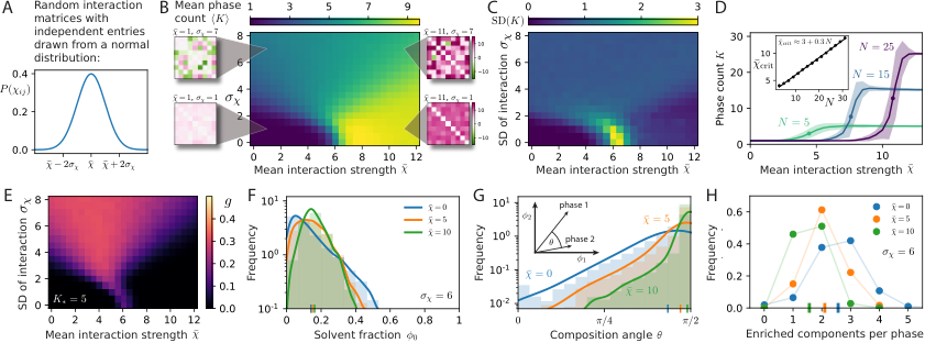
To gain intuition for the behavior of the multicomponent system, we first consider random interaction matrices . To compare with the literature Sear and Cuesta 2003; Jacobs and Frenkel 2013; Jacobs and Frenkel 2017; Shrinivas and Brenner 2021; Jacobs 2021, we draw entries independently from a normal distribution with mean and variance ; see Fig. 2A. For each parameter pair , we investigate realizations of and initial compositions and summarize the resulting distribution by its mean and standard deviation. Fig. 2B shows that only a single phase forms when interactions are generally weak (low and ), consistent with an ideal solution where entropy favors mixing. When interactions are increased without strong variations (larger , low ), a demixing transition happens at , and phases are typical at large . Here, all components segregate from each other and form separate phases, each enriched in a single component. Fig. 2C shows that the width of the phase count distribution, , is largest in the transition zone, indicating that the actually observed strongly depends on the chosen interaction matrix and initial composition. The critical value , where the demixing transition takes places, increases with the component count (see Fig. 2D), which confirms a trend that was observed in earlier work Jacobs and Frenkel 2017; Sear and Cuesta 2003. Fig. 2B also shows that the width of the transition zone is generally broader for larger , consistent with the fact that interactions are more variable. Interestingly, the statistics of the phase count become independent of for large variations . In this case, we observe , which was previously conjectured for Shrinivas and Brenner 2021. Taken together, our simplified dynamics are consistent with known results for random matrices.
The results shown in Fig. 2B indicate that random interactions of components can lead to approximately , , and phases in large regions of the parameter space, while other values require fine-tuning. Even if it is possible to find parameters and that on average lead to a desired phase count , it will not always be reached since the actual distribution of the number of phases, , possesses a significant width; see Fig. 2C. To quantify how well the system reaches a target phase count , we define the performance
| (5) |
which is constructed such that and if and only if all initial conditions lead to phases. Here, controls how strongly deviations from the target are punished; see Fig. 1E. Fig. 2E shows that the maximal performance of the random ensemble is , even though the choice is close to , so large leads to . Indeed, supplementary Fig. S2 shows that the random ensemble performs even worse for other targets . Taken together, it is thus not sufficient to vary the two parameters and of the random interactions to obtain a particular phase count reliably.
Equilibrium phases resulting from random interactions also show strong composition variations. For instance, the solvent fraction varies between and (Fig. 2F). We quantify differences of phase compositions using the composition angle , which is simply the angle between the composition vectors of two phases and Shrinivas and Brenner 2021; see inset of Fig. 2G. Note that is zero when phases have identical composition (but not necessarily the same total concentration) while when compositions are orthogonal, i.e., when they have no components in common. While compositions of initial phases are similar (see Supporting Fig. S1B), they typically become very different after equilibration; see Fig. 2G. In particular, the mean difference increases with stronger repulsion (larger ). However, even for the strongest repulsion, there is significant overlap between phases, indicating that components are not cleanly sorted into distinct phases. To quantify this, we count for each phase how many components have a fraction larger than times the average fraction. The number of such enriched components is smaller for stronger interactions, although it varies widely; see Fig. 2H. Taken together, typical random interaction matrices cannot provide a reliable phase count , so some additional structure is required.
Naively structured interactions also do not lead to reliable phase counts

To elucidate what structure in interaction matrices reliably leads to a desired phase count , we next group the interacting components in clusters. We impose a repulsive interaction between components belonging to different clusters, while components within a cluster exhibit a weak interaction . We expect that components in the same cluster co-segregate, so the system behaves as if it consisted of effective components that all repel each other with strength . Indeed, Fig. 3A shows that demixing into many phases happens when is sufficiently large, while the intra-cluster interaction has a weaker effect. Co-segregation even takes place when the intra-cluster interaction is slightly repulsive (). However, while these designed matrices display expected behavior, they still have significant variations and the resulting performance is only marginally better than that of random matrices (Fig. 3B). This is also visible in the distribution of the composition angles shown in Fig. 3C: Even for strong repulsion (large ) there is a significant fraction of phases with similar composition (), even though exactly two components are enriched in each phase (Fig. 3D). It seems as if weakly concentrated components, including the solvent, prevent reliable co-segregation of clustered components. We thus find that creating interaction matrices with desired behavior is not as straight-forward as we had hoped.
Evolutionarily optimized interactions lead to reliable phase counts
Neither completely random nor fully structured interaction matrices are very realistic in biology since the interaction energies summarize complex interactions of proteins Dignon et al. 2020, which change continuously during evolution Schuster et al. 2020. We thus next ask whether an evolutionary optimization of interaction matrices can reliably lead to mixtures with a particular target phase count .
To mimic biology, we evolve an ensemble of individuals, characterized by interaction matrices , over multiple generations. We initialize a population of individuals with randomly chosen interaction matrices using and . For each individual, we numerically determine and the associated performance , see Eq. (5), which will now play the role of a fitness. In the selection step, we remove the of the population with lowest performance, replacing them by randomly chosen high-performance individuals to maintain population size. We then mutate the interactions of all individuals by adding independent random numbers from a normal distribution with zero mean and standard deviation . Repeating this procedure for many generations improves the performance of all individuals, so that they reliably reach the target . However, we also noticed that this naive optimization results in very large interaction magnitudes (see Supporting Fig. S3), which might be unrealistic. To prevent such unphysical behavior, we additionally scale the interaction matrix by if its mean absolute value exceeds the threshold . This limits the average interaction magnitude, , but the evolutionary optimization still discovers interaction matrices with a precise phase count (Fig. 4A) and perfect performance (Fig. 4B). Optimized interaction matrices thus vastly outperform random matrices and allows targeting specific phase counts despite strong fluctuations in initial composition.

The outstanding performance of evolved interaction matrices is surprising since we limited the interaction magnitude (Fig. 4C) and use highly variable initial compositions. What properties of lead to the excellent performance ? Simply visualizing optimized interaction matrices (Fig. 4E) does not reveal any obvious structure. In any case, we showed in Fig. 3 that block matrices are not optimal, so any obvious clustering might actually be detrimental. The distribution of the entires in optimized interaction matrices is very broad (Fig. 4F), although its width is directly limited by our constraint of . For sufficiently large , the distribution is well-described by a normal distribution (dotted blue line). This is surprising, since unstructured random matrices chosen from such a normal distribution did not perform well (Fig. 2). The similarity to the random ensemble also shows in the distribution of the solvent fraction (compare Fig. 4F to Fig. 2F) and the number of enriched components (compare Fig. 4H to Fig. 2H). In contrast, the distribution of composition angles is slightly different (compare Fig. 4G to Fig. 2G). However, is larger for the random ensemble with large , implying more distinct phases. Taken together, optimized matrices share many similarities with random matrices, although minute differences apparently lead to a much improved performance.
The evolutionary optimization quickly discovered interaction matrices that lead to a reliable phase count and these matrices evolve continuously. This begs the question whether this task is actually difficult; how frequent are optimal matrices in the space of all matrices? Our analysis of random matrices clearly showed that matrices must fulfill some basic requirements to have a phase count close to the target . In particular, the average magnitude of the entries and the associated standard deviation need to be chosen such that ; see Fig. 2B. While we showed that the ensemble of random matrices with these properties does not work optimally (Fig. 2E), individual matrices from the ensemble might perform well. To quantify this, we determined the performance for random matrices characterized by a particular choice of and . Supplementary Fig. S4 shows that we easily discover matrices with high performance. This implies that a large fraction of all matrices with suitable statistics, determined by and , performs optimally.
Performance of evolutionarily optimized interactions is robust
We showed that interaction matrices leading to exactly phases can be obtained through random trial-and-error or by evolutionary optimization. This situation corresponds to maximizing the performance in a fixed environment without any fluctuations beyond the initial composition. However, biological systems constantly face additional fluctuations, both internally (e.g., changes of the component count) and externally (e.g., changing environment). Such systems need to work not only in a particular case, but they need to be robust to these fluctuations, too. To see how evolution of multicomponent phase separation fares in such challenging situations, we next study the dynamics when interaction matrix , the number of components, or the target phase count varies.
We start by perturbing a single component in the evolutionarily optimized interaction matrices by choosing a random row (and column) to which we add uncorrelated random numbers from a normal distribution of vanishing mean and standard deviation . Fig. 5A shows that the performance of optimized matrices is only weakly affected for , while larger perturbations reduce the performance significantly. Mixtures with more components are more sensitive to these perturbations, presumably because our procedure modifies the interaction between the chosen component and all other ones, so larger mixtures exhibit more perturbations. Taken together, we find that optimized mixtures still form phases reliably even when interaction energies are perturbed by .
We next test the robustness of the system against changes in component count itself, which captures gene loss and duplication in real systems. We quantify the effect of changing by measuring the performance when one of the components of the optimized interactions matrices is removed or duplicated. Fig. 5B shows that removing a component reduces the performance substantially, although the reduction is smaller for larger . Conversely, duplicating a component has hardly any effect on performance. Taken together, this suggests that using more components to form a fixed number of phases is more robust to internal fluctuations, like variations in component count.
We next consider external fluctuations of the environment. Since we do not model the environment explicitly, we consider changes of the target phase count , assuming that the environment changes such that organisms need to form fewer or more phases. Changing by one will necessarily reduce the performance from the optimal value to ; see Eq. (5). To see how well different systems adapt to new environments, we study how quickly the performance recovers under the evolutionary dynamics. Fig. 5C shows that individuals quickly adjust to a lower target count, although the generation at which this happens varies widely; see inset. This adaptation tends to be a bit slower for more components, presumably because more interactions have to be adjusted. Conversely, adaptation to an increased target count is easier for more components; see Fig. 5D. Note that the smallest system with does not succeed to meet the target reliably due to the constraint on . Taken together, this suggests that there is a larger flexibility in the phase composition at larger , which allows to quickly find an interaction matrix resulting in an additional phase. Reducing the phase count is more complicated, likely because many interactions have to be adjusted. In fact, there is a trade-off between robustly reaching a constant phase count despite perturbations and using the same perturbations to flexibly adjust to new environments.

Discussion
Understanding the equilibrium properties of biomolecules is crucial before we can tackle the more challenging problem of a living system. We here proposed a novel method to study how the many interacting constituents of a cell spontaneously segregate into different phases. This method recovers the demixing transition that was previously observed when many components exhibit random interactions Jacobs and Frenkel 2017; Shrinivas and Brenner 2021. We also find a variable phase count for a given set of interactions, which is a signature of the complex phase diagrams Mao et al. 2018. Beyond these limiting cases, our method can efficiently handle arbitrary interactions involving several tens of different components, thus increasing the range of systems that can be studied.
We use our method to optimize interaction matrices to yield a precise phase count. These optimized interactions are also robust to perturbations and allow a fast adaption to an increased target phase count, particularly if many components are involved. In contrast, forming fewer phases seems to be more challenging for larger mixtures, presumably because these mixtures are actually robust to perturbations. It will be interesting to study this trade-off between robustness and evolvability in more detail in the future.
Optimal interaction matrices are surprisingly easy to discover and even random matrices have a high chance of yielding a robust number of phases, which is independent of the initial composition. On the contrary, other random matrices from the same ensemble perform much worse. What are properties that separate the optimal matrices from generic ones? Answering this question is directly relevant to biomolecular condensates, where hidden structures in intrinsically disordered regions might strongly affect the phase behavior of proteins Moses et al. 2021. Our method can also be extended to describe more complex behavior of biomolecular condensates, including response to external cues Choi et al. 2020; Adame-Arana et al. 2020, active regulation Hondele et al. 2020; Soeding et al. 2020; Kirschbaum and Zwicker 2021, and noise buffering Klosin et al. 2020; Deviri and Safran 2021. Ultimately, our predictions could be tested using engineered condensates Bracha et al. 2019 and quantitative reconstitution Currie and Rosen 2021. Beside these concrete applications for biomolecular condensates, our method might also answer more fundamental questions about evolving systems: How can a cell exhibit robust functions while its proteins evolve Laan et al. 2015; Diepeveen et al. 2018; Brauns et al. 2020? We hope that our abstract model will illuminate the fundamental problem of how variable microscopic interactions lead to robust collective properties.
Acknowledgements.
We thank Evan Spruijt for a critical review of the manuscript and helpful discussions. D.Z. acknowledges funding by the Max Planck Society. L.L. gratefully acknowledges funding from the European Research Council (ERC) under the European Union’s Horizon 2020 research and innovation programme (Grant agreement No. 758132 and funding from the Netherlands Organization for Scientific Research (Nederlandse Organisatie voor Wetenschappelijk Onderzoek; NWO) through a VIDI grant (016.Vidi.171.060).Appendix A Derivation of simple dynamical system
We here give a detailed derivation of the simple dynamical system that we use in the main text to determine equilibrium states of the multicomponent liquid. In particular, we demonstrate below that the stationary states of this dynamical system correspond to actual equilibrium solutions.
A.1 Equilibrium conditions of the physical system
The conditions for an equilibrium between two phases and are given by Eq. (3) in the main text. The non-dimensional chemical potentials and pressures are
| (6a) | ||||
| (6b) | ||||
In general, the multiphase system is specified by the phase volumes together with either all particle numbers, , or all volume fractions . Here, and are extensive quantities that grow with system size, while the fractions are the intensive quantities that appear in Eq. (3) and Eq. (6b).
A.2 Dynamics of the full physical system
To determine the equilibrium states satisfying Eqs. (3), we first discuss the dynamics of the physical system, specified by the intensive quantities together with the extensive volumes of all phases. We can then express the rate of change of the free energy as
| (7) |
Here, we consider the spontaneous relaxation to equilibrium, implying dynamics that decrease continuously, . Using linear non-equilibrium thermodynamics Jülicher et al. 2018, one can show that the exchange of volume is driven by pressure differences and differences in chemical potential imply changes in particle numbers,
| (8a) | ||||
| (8b) | ||||
where the kinetic coefficients and need to be symmetric, and . We can use this together with Eq. (7) to show explicitly that the free energy cannot increase under these conditions,
| (9) |
This implies that the following three statements about the system’s state are all equivalent: (i) is at a stationary point, ; (ii) The dynamics given in Eq. (8) are at a stationary point; (iii) The system fulfills the equilibrium conditions Eq. (3) and the volume and particle number constraints. We can thus determine solutions to Eq. (3) using the dynamics given in Eq. (8) to relax initial conditions to a stationary state.
A concrete implementation of the relaxation dynamics requires sensible choices for the kinetic coefficients. We use and , where we introduced the relaxation rate , which defines the non-dimensional time . Using , the dynamics of the system read
| (10a) | ||||
| (10b) | ||||
These equations define an initial value problem, which relaxes an initial configuration, and , toward equilibrium.
A.3 Simplified dynamical system
The physical dynamics defined by Eq. (10) involve both the intensive fractions and the extensive volumes . However, the equilibrium conditions (3) are local statements about the coexistence of phases and thus do not involve extensive quantities. To solve only the coexistence problem, we now seek a dynamical system that only involves intensive variables. Inspecting Eq. (10b), we see that the volumes only affect the rate at which the fractions change but not the direction of change. Consequently, we obtain qualitatively similar dynamics by removing the pre-factor, which results in Eq. (4). Clearly, equilibrium states, which fulfill Eq. (3), are stationary states of Eq. (4). We next demonstrate that the stationary state conditions of Eq. (4) also imply the equilibrium conditions Eq. (3). To do this, we introduce the deviations
| (11) |
from the means , , and . Using this, we can give the equilibrium conditions as conditions,
| (12) |
with constraints, , resulting in independent conditions. In contrast, we have conditions for the stationary state,
| (13) |
Summing Eq. (13) over , we find , which implies
| (14) |
Note that these are only independent equations since . There are additional equations that follow from Eq. (13), resulting in independent equations describing the stationary state,
| (15a) | ||||
| (15b) | ||||
To show that these are equivalent to the equilibrium conditions (12), we express them as a linear system,
| (16) |
where
| (17) |
has entries, and
is a matrix of blocks where each block has the dimension , except in the last column, where the blocks have dimension . The block size can thus be summarized as
| (23) |
Clearly, this matrix has rows and columns, so it is a square matrix if and only if .
To show that the stationary state conditions given in Eq. (13) imply the equilibrium conditions Eq. (12), we need to show that the linear system given in Eq. (16) only has the trivial solution . If is a square matrix, this amounts to showing that its determinant is non-zero. We will show below that the non-square case can be treated by investigating the largest square sub matrix , which is built by dropping the last rows or columns. Defining the relevant dimension , the determinant of this matrix reads
| (24) |
where we defined the square composition matrix
| (25) |
Note that the determinant of only vanishes if , since . In the following, we analyze the solution space for the three relevant dimensional cases.
A.3.1 Balanced case of a square matrix
In the balance case, , we have and describes the full composition. The linear system could have non-trivial solutions if the determinant of vanishes. Generally, vanishes if rows or columns are linearly dependent. This is for instance the case when two phases have identical composition, for two phases and all components . However, in this case the conditions and are trivially fulfilled, so we can always ignore identical phases and instead focus on phases with distinct composition. The determinant also vanishes when two species have identical composition in all phases, for some and all . This is only possible if they behave identically, for all , in which case we again find and . In this case, the two components can basically be treated as one and thus also ignored. Generally, the determinant also vanishes when a row (column) can be written as a linear sum of the other rows (columns). While we could not identify a mathematical statement that this is impossible, we never observed such a case and will thus not discuss it further. Taken together, we conclude that the stationary state conditions Eq. (13) imply the equilibrium conditions Eq. (12) if .
A.3.2 Overdetermined case of few phases
In this case, has more rows than columns, so there are more stationary state conditions than equilibrium conditions. This implies , , and . By solving the square sub-problem involving , we find . In doing so, we ignored the extra conditions
| (26) |
but these are trivially fulfilled. Taken together, this shows that the overdetermined case implies .
A.3.3 Underdetermined case of too many phases
In this case, has more columns than rows, , , and . This implies that there are not sufficient stationary state conditions to immediately conclude that the equilibrium conditions hold. However, the variables and are not truly independent since they are both functions of the composition ; see Eq. (6b). Combining these conditions, we find
| (27) |
for all , demonstrating a linear relationship between and that depends non-linearly on . Since these conditions must also hold, it is plausible that only of the unknowns of the linear system (16) are independent. Assuming this is the case, we can solve the linear subsystem of dimensions, whose determinant is given in Eq. (6b). Similarly to the cases discussed above, this system has only the trivial solutions, implying that for the first unknowns. This shows that most equilibrium conditions follow from the stationary state conditions in the underdetermined case and suggests that the stationary state system does not possess any solutions that violate the equilibrium conditions. Indeed, we never observed any numerical solutions of the stationary state conditions (13) that violated the equilibrium conditions (12).
Note that the underdetermined system is related to Gibbs’ phase rule, which implies that at most phases can have different composition Gibbs 1876. Consequently, the number of undetermined variables we encountered here is exactly the minimal number of phases that needs to have a composition equivalent to other phases. The additional constraints introduced by the fact that and all depend on thus reflect the thermodynamic stability discussed by Gibbs.
Appendix B Numerical solution method
We solve Eq. (4) using an explicit scheme with adaptive time stepping; see source code sou 2022. Since the simulation typically converges exponentially, we conclude that a stationary state has been reached when all . For each choice of , we run simulations with random initial conditions to estimate the distribution of the phase count , which is the minimal number of points so that for all phases .
We choose initial conditions for a phase such that all admissible composition vector including the solvent fraction exhibit a uniform distribution. Here, we obviously use and we ensure for . The condition that all fractions sum to one implies correlations between the fractions, but since the geometry of allowed fractions is a simplex in an -dimensional space, we can determine the marginal distributions along each dimension and choose the fractions iteratively. We use the conditional probabilities
| (28a) | ||||
| (28b) | ||||
| (28c) | ||||
| (28d) | ||||
where
| (29) |
is a particular, scaled Beta distribution defined for . These conditional probabilities given in Eqs. (28) allow us to draw random variates of , since we can sample from the one-dimensional distributions for one after another. Note that the joint probability distribution reads
| (30) |
and is thus constant, demonstrating that this is truly a uniform distribution. Fig. S1 shows statistics of these initial compositions.
To demonstrate the procedure, we consider the example , where we have and , implying . The expectation values are
| (31a) | ||||
| (31b) | ||||
| (31c) | ||||
demonstrating that indeed all three components have identical average fraction.
References
- Brangwynne et al. [2009] C. P. Brangwynne, C. R. Eckmann, D. S. Courson, A. Rybarska, C. Hoege, J. Gharakhani, F. Jülicher, and A. A. Hyman, Science 324, 1729 (2009).
- Feric et al. [2016] M. Feric, N. Vaidya, T. S. Harmon, D. M. Mitrea, L. Zhu, T. M. Richardson, R. W. Kriwacki, R. V. Pappu, and C. P. Brangwynne, Cell 165, 1686 (2016).
- Banani et al. [2017] S. F. Banani, H. O. Lee, A. A. Hyman, and M. K. Rosen, Nat. Rev. Mol. Cell Biol. 18, 285 (2017).
- Azaldegui et al. [2020] C. A. Azaldegui, A. G. Vecchiarelli, and J. S. Biteen, Biophys. J. 120, 1123 (2020).
- Cohan and Pappu [2020] M. C. Cohan and R. V. Pappu, Trends Biochem Sci 45, 668 (2020).
- Greening and Lithgow [2020] C. Greening and T. Lithgow, Nat. Rev. Microbiol. 18, 677 (2020).
- Emenecker et al. [2021] R. J. Emenecker, A. S. Holehouse, and L. C. Strader, Annu. Rev. Plant Biol. 72, 10.1146/annurev-arplant-081720-015238 (2021), pMID: 33684296.
- Kim et al. [2021] J. Kim, H. Lee, H. G. Lee, and P. J. Seo, EMBO reports 22, e51656 (2021).
- Lafontaine et al. [2020] D. L. J. Lafontaine, J. A. Riback, R. Bascetin, and C. P. Brangwynne, Nat. Rev. Mol. Cell Biol. 22, 165 (2020).
- Fei et al. [2017] J. Fei, M. Jadaliha, T. S. Harmon, I. T. S. Li, B. Hua, Q. Hao, A. S. Holehouse, M. Reyer, Q. Sun, S. M. Freier, R. V. Pappu, K. V. Prasanth, and T. Ha, J. Cell Sci. 130, 4180 (2017).
- Fritsch et al. [2021] A. W. Fritsch, A. F. Diaz-Delgadillo, O. Adame-Arana, C. Hoege, M. Mittasch, M. Kreysing, M. Leaver, A. A. Hyman, F. Jülicher, and C. A. Weber, Proc. Natl. Acad. Sci. USA 118, 10.1073/pnas.2102772118 (2021).
- Dignon et al. [2020] G. L. Dignon, R. B. Best, and J. Mittal, Annu. Rev. Phys. Chem. 71, 53 (2020).
- Hardenberg et al. [2020] M. Hardenberg, A. Horvath, V. Ambrus, M. Fuxreiter, and M. Vendruscolo, Proc. Natl. Acad. Sci. USA 117, 33254 (2020).
- Adekunle and Hubstenberger [2020] D. A. Adekunle and A. Hubstenberger, Emerg Top Life Sci 4, 265 (2020).
- Lyon et al. [2020] A. S. Lyon, W. B. Peeples, and M. K. Rosen, Nat. Rev. Mol. Cell Biol. 22, 215 (2020).
- Jin et al. [2021] X. Jin, J.-E. Lee, C. Schaefer, X. Luo, A. J. M. Wollman, A. L. Payne-Dwyer, T. Tian, X. Zhang, X. Chen, Y. Li, T. C. B. McLeish, M. C. Leake, and F. Bai, Sci. Adv. 7, eabh2929 (2021).
- Alberti and Dormann [2019] S. Alberti and D. Dormann, Annu. Rev. Genet. 53, 171 (2019), pMID: 31430179.
- Saar et al. [2021] K. L. Saar, A. S. Morgunov, R. Qi, W. E. Arter, G. Krainer, A. A. Lee, and T. P. J. Knowles, Proc. Natl. Acad. Sci. USA 118, 10.1073/pnas.2019053118 (2021).
- Choi et al. [2020] J.-M. Choi, A. S. Holehouse, and R. V. Pappu, Annu. Rev. Biophys. 49, 107 (2020).
- Harmon et al. [2017] T. S. Harmon, A. S. Holehouse, M. K. Rosen, and R. V. Pappu, Elife 6, 10.7554/eLife.30294 (2017).
- Lin et al. [2018] Y.-H. Lin, J. D. Forman-Kay, and H. S. Chan, Biochemistry 57, 2499 (2018).
- Schuster et al. [2020] B. S. Schuster, G. L. Dignon, W. S. Tang, F. M. Kelley, A. K. Ranganath, C. N. Jahnke, A. G. Simpkins, R. M. Regy, D. A. Hammer, M. C. Good, et al., Proc. Natl. Acad. Sci. USA 117, 11421 (2020).
- Bremer et al. [2021] A. Bremer, M. Farag, W. M. Borcherds, I. Peran, E. W. Martin, R. V. Pappu, and T. Mittag, Nat. Chem. 10.1038/s41557-021-00840-w (2021).
- Hyman et al. [2014] A. A. Hyman, C. A. Weber, and F. Jülicher, Annu. Rev. Cell Dev. Biol. 30, 39 (2014).
- Brangwynne et al. [2015] C. P. Brangwynne, P. Tompa, and R. V. Pappu, Nat. Phys. 11, 899 (2015).
- Berry et al. [2018] J. Berry, C. Brangwynne, and M. P. Haataja, Rep. Prog. Phys. 81, 046601 (2018).
- Weber et al. [2019] C. A. Weber, D. Zwicker, F. Jülicher, and C. F. Lee, Rep. Prog. Phys. 82, 064601 (2019).
- Riback et al. [2020] J. A. Riback, L. Zhu, M. C. Ferrolino, M. Tolbert, D. M. Mitrea, D. W. Sanders, M.-T. Wei, R. W. Kriwacki, and C. P. Brangwynne, Nature 581, 209 (2020).
- Mao et al. [2018] S. Mao, D. Kuldinow, M. Haataja, and A. Kosmrlj, Soft Matter 15, 1297 (2018).
- Mao et al. [2020] S. Mao, M. S. Chakraverti-Wuerthwein, H. Gaudio, and A. Košmrlj, Phys. Rev. Lett. 125, 218003 (2020).
- Leung et al. [2003] A. K. L. Leung, J. S. Andersen, M. Mann, and A. I. Lamond, Biochem. J 376, 553 (2003).
- Updike and Strome [2009] D. L. Updike and S. Strome, Genetics 183, 1397 (2009).
- Currie and Rosen [2021] S. L. Currie and M. K. Rosen, RNA 28, 27 (2021).
- Banani et al. [2016] S. F. Banani, A. M. Rice, W. B. Peeples, Y. Lin, S. Jain, R. Parker, and M. K. Rosen, Cell 166, 651 (2016).
- Zhou and Xie [2021] S. Zhou and Y. M. Xie, International Journal of Mechanical Sciences 198, 106349 (2021).
- Shrinivas and Brenner [2021] K. Shrinivas and M. P. Brenner, Proc. Natl. Acad. Sci. USA 118, 10.1073/pnas.2108551118 (2021).
- Sear and Cuesta [2003] R. P. Sear and J. Cuesta, Physical Review Letters, Phys. Rev. Lett. 91, 245701 (2003).
- Jacobs and Frenkel [2013] W. M. Jacobs and D. Frenkel, The Journal of Chemical Physics, J. Chem. Phys. 139, 024108 (2013).
- Jacobs and Frenkel [2017] W. M. Jacobs and D. Frenkel, Biophys. J. 112, 683 (2017).
- Jacobs [2021] W. M. Jacobs, Phys. Rev. Lett. 126, 258101 (2021).
- Gibbs [1876] J. W. Gibbs, Transactions of the Connecticut Academy of Arts and Sciences, Trans. Conn. Acad. Arts Sci. 3, 1 (1876).
- Flory [1942] P. I. Flory, The Journal of Chemical Physics, J. Chem. Phys. 10, 51 (1942).
- Cahn and Hilliard [1958] J. W. Cahn and J. E. Hilliard, J. Chem. Phys. 28, 258 (1958).
- Xu et al. [2014] X. Xu, C. L. Ting, I. Kusaka, and Z.-G. Wang, Annu. Rev. Phys. Chem. 65, 449 (2014), pMID: 24689799.
- Shimobayashi et al. [2021] S. F. Shimobayashi, P. Ronceray, D. W. Sanders, M. P. Haataja, and C. P. Brangwynne, Nature 599, 503 (2021).
- Moses et al. [2021] D. Moses, K. Guadalupe, F. Yu, E. Flores, A. Perez, R. L. McAnelly, N. M. Shamoon, E. Cuevas-Zepeda, A. Merg, E. W. Martin, A. S. Holehouse, and S. Sukenik, bioRxiv 10.1101/2021.11.24.469609 (2021).
- Adame-Arana et al. [2020] O. Adame-Arana, C. A. Weber, V. Zaburdaev, J. Prost, and F. Jülicher, Biophysical Journal, Biophys. J. 119, 1590 (2020).
- Hondele et al. [2020] M. Hondele, S. Heinrich, P. De Los Rios, and K. Weis, Emerg. Top. Life Sci. 4, 343 (2020).
- Soeding et al. [2020] J. Soeding, D. Zwicker, S. Sohrabi-Jahromi, M. Boehning, and J. Kirschbaum, Trends Cell Biol. 30, 4 (2020).
- Kirschbaum and Zwicker [2021] J. Kirschbaum and D. Zwicker, J. R. Soc. Interface 18, 20210255 (2021).
- Klosin et al. [2020] A. Klosin, F. Oltsch, T. Harmon, A. Honigmann, F. Jülicher, A. A. Hyman, and C. Zechner, Science 367, 464 (2020).
- Deviri and Safran [2021] D. Deviri and S. A. Safran, Proc. Natl. Acad. Sci. USA 118, 10.1073/pnas.2100099118 (2021).
- Bracha et al. [2019] D. Bracha, M. T. Walls, and C. P. Brangwynne, Nat. Biotechnol. 37, 1435 (2019).
- Laan et al. [2015] L. Laan, J. H. Koschwanez, and A. W. Murray, eLife 4, e09638 (2015).
- Diepeveen et al. [2018] E. T. Diepeveen, T. Gehrmann, V. Pourquié, T. Abeel, and L. Laan, Genome Biology and Evolution 10, 1765 (2018).
- Brauns et al. [2020]
F. Brauns, L. M. I
textasciitilde nigo de la Cruz, W. K.-G. Daalman, I. de Bruin, J. Halatek, L. Laan, and E. Frey, bioRxiv 10.1101/2020.09.09.290510 (2020). - Jülicher et al. [2018] F. Jülicher, S. W. Grill, and G. Salbreux, Rep. Prog. Phys. 81, 076601 (2018).
- sou [2022] Project source code, https://github.com/zwicker-group/paper-multicomponent-evolution (2022).

