跳到论文正文
W Papers独立论文阅读器 arXiv:2201.10658 论文正文 计算阅读时间 · 0%
引用这篇论文根据当前论文元数据生成,正式投稿前建议核对。


License: arXiv.org perpetual non-exclusive license
arXiv:2201.10658v1 [math.NA] 25 Jan 2022

P1P_{1}–Nonconforming Quadrilateral Finite Element Space with Periodic Boundary Conditions:
Part I. Fundamental results on dimensions, bases, solvers, and error analysis

Jaeryun Yim Email: jaeryun.yim@gmail.com Thanks: Interdisciplinary Program in Computational Science & Technology, Seoul National University, Seoul 08826, Korea; current address: Encored Technologies, 215 Bongeunsa-ro, Gangnam-gu, Seoul 06109, Korea.    Dongwoo Sheen Email: sheen@snu.ac.kr Thanks: Department of Mathematics, Seoul National University, Seoul 08826, Korea.
Abstract

The P1P_{1}–nonconforming quadrilateral finite element space with periodic boundary condition is investigated. The dimension and basis for the space are characterized with the concept of minimally essential discrete boundary conditions. We show that the situation is totally different based on the parity of the number of discretization on coordinates. Based on the analysis on the space, we propose several numerical schemes for elliptic problems with periodic boundary condition. Some of these numerical schemes are related with solving a linear equation consisting of a non-invertible matrix. By courtesy of the Drazin inverse, the existence of corresponding numerical solutions is guaranteed. The theoretical relation between the numerical solutions is derived, and it is confirmed by numerical results. Finally, the extension to the three dimensional is provided.

keywords
Finite element method, nonconforming, periodic boundary condition.
††corref: cor:dim-equation
AMS
65N30

1 Introduction

Many macroscopic material properties are obtained from the knowledge of accurate microscopic material properties. However in most realistic cases the ratio of macro scale to micro scale is so large that it cannot be directly computed the dynamics described at the microscale level. Therefore usually upscaling techniques are used to reduce the micro scale level computation to approximately obtain macroscopic properties. Recently, several efficient multiscale methods have been developed towards that direction. These include numerical homogenization [4, 5, 13, 14], MsFEM (multiscale finite element methods) and GMsFEM (generalized MsFEM) [12, 10, 11, 17], VMS (variational multiscale finite element methods) [18], MsFVM (multiscale finite volume methods) [20] and HMM (heterogeneous multiscale methods) [1, 9]. In numerical homogenization and upscaling of multiscale problems one often needs to solve periodic boundary value problems at microscale level efficiently.

The P1P_{1}–nonconforming quadrilateral finite element [27] has an advantage in computing stiffness matrice as the gradient of linear polynomials is constant in each quadrilateral as well as it has the smallest number of DOFs (degrees of freedom) for given quadrilateral mesh. There have been a number of studies about this finite element for fluid dynamics, elasticity, electromagnetics [23, 15, 25, 24, 26, 28, 8, 16]. Unlikely other finite elements, this space is strongly tied with the boundary condition for given problem due to the dice rule constraint element by element (See (3.1)). Most of those works are focused on the finite element space with Dirichlet and/or Neumann BCs. Altmann and Carstensen [2] show the dimension of, and a basis for the finite element space with inhomogeneous Dirichlet BCs which shares similar discrete nature with the Neumann boundary case.

On the other hand, the P1P_{1}-nonconforming quadrilateral element space with periodic BC has not been investigated. Thus, it is our intention to investigate its dimension and basis with periodic BC.

The discrete formulation of periodic problems yields singular linear systems, which can be dealt with various kinds of generalized inverses of a matrix. Among them, we will concentrate on the Drazin inverse, as it can be expressed as a matrix polynomial, since the Krylov method, which is based on the same idea on matrix polynomials, can be applied to singular linear systems. One of the most important properties of the Drazin inverse is the expressibility it as a polynomial in the given matrix. The Krylov iterative method for a nonsingular linear system is established on this property. The Krylov scheme can be applied to a singular linear system as well under proper consistency conditions [19, 22, 30, 7, 3, 6].

The aim of this paper is to investigate the structure of the P1P_{1}–nonconforming quadrilateral finite element spaces with periodic BC thoroughly and to suggest some iterative methods to solve the resulting linear systems based on the idea of Drazin inverse. An application for nonconforming heterogeneous multiscale methods (NcHMM) of P1P_{1}–nonconforming quadrilateral finite element will appear in [29].

The organization of the paper is as follows. In Section 2, we give a brief explanation for the P1P_{1}–nonconforming quadrilateral finite element and the Drazin inverse. We investigate the dimension of the finite element spaces with various BCs, including periodic condition which is our main concern, in Section 3. We introduce the concept of minimally essential discrete BCs to analyze the precise effects of given BC on the dimension of the corresponding finite element space. In Section 4, a basis for the periodic nonconforming finite element space is constructed. It consists of node-based functions by identifying boundary node-based functions in a suitable way and a complementary basis consisting of a few alternating functions is considered. We propose several numerical schemes for solving a second-order elliptic problem with periodic BC in Section 5. We use an efficient iterative method based on the Krylov space in help of the Drazin inverse of the corresponding singular matrix. The relationship between solutions of the schemes will be discussed. Finally, we extend all our results to the 3D case in Section 6.

2 Preliminaries and notations

In this section some basics on the Drazin inverse and the P1P_{1}–nonconforming quadrilateral finite element will be briefly reviewed. Also notations to be used are described.

2.1 The Drazin inverse

Let AA be a linear transformation on ℂn\mathbb{C}^{n}. The index of AA, denoted by Ind⁡(A),\operatorname{Ind}\,(A), is defined as the smallest nonnegative integer kk such that

Im⁡A0⊃Im⁡A⊃⋯⊃Im⁡Ak−1⊃Im⁡Ak=Im⁡Ak+1=⋯,\operatorname{Im}A^{0}\supset\operatorname{Im}A\supset\cdots\supset\operatorname{Im}A^{k-1}\supset\operatorname{Im}A^{k}=\operatorname{Im}A^{k+1}=\cdots,

or equivalently

ker⁡A0⊂ker⁡A⊂⋯⊂ker⁡Ak−1⊂ker⁡Ak=ker⁡Ak+1=⋯.\ker A^{0}\subset\ker A\subset\cdots\subset\ker A^{k-1}\subset\ker A^{k}=\ker A^{k+1}=\cdots.

It yields that, restricted on Im⁡Ak\operatorname{Im}A^{k}, the transformation AA becomes an invertible linear transformation. The Drazin inverse of AA, denoted by ADA^{D}, is defined as follows: for u=v+w∈ℂnu=v+w\in\mathbb{C}^{n} where v∈Im⁡Akv\in\operatorname{Im}A^{k} and w∈ker⁡Akw\in\ker A^{k}, AD​u:=A|Im⁡Ak−1​vA^{D}u:=\left.A\right|_{\operatorname{Im}A^{k}}^{-1}v. One of the most important properties of the Drazin inverse matrix of AA is that it is expressible as a polynomial in AA:

Theorem 1 ([7]).

If A∈ℂn×nA\in\mathbb{C}^{n\times n}, then there exists a polynomial p⁡(x)p(x) such that AD=p⁡(A)A^{D}=p(A).

For a singular matrix A,A, a unique Drazin inverse solution can be found by using the Krylov iterative method under some proper consistency conditions. For details, see [7, 19].

Theorem 2 ([19]).

Let mm be the degree of the minimal polynomial for AA, and let kk be the index of AA. If b∈Im⁡Akb\in\operatorname{Im}A^{k}, then the linear system A​x=bAx=b has a unique Krylov solution x=AD​b∈𝒦m−k​(A,b)x=A^{D}b\in\mathcal{K}_{m-k}(A,b). If b∉Im⁡Akb\not\in\operatorname{Im}A^{k}, then A​x=bAx=b does not have a solution in the Krylov space 𝒦n​(A,b)\mathcal{K}_{n}(A,b).

2.2 Notations

For d=2d=2 or 3,3, let Ω=Πj=1d​(0,ℓj)⊂ℝd\Omega=\Pi_{j=1}^{d}(0,\ell_{j})\subset\mathbb{R}^{d} denote a dd-dimensional rectangular domain. Let (𝒯h)0<h<minj=1d⁡(ℓj)({\mathcal{T}}_{h})_{0<h<\min_{j=1}^{d}(\ell_{j})} be the quasiuniform family of triangulations of Ω\Omega into dd–dimensional polyhedral subdomains QhQ_{h}’s which are convex and topologically equivalent to dd–dimensional cubes, with maximum diameter bounded by the mesh parameter h.h. We further assume that, for 0<h<minj=1d⁡(ℓj),{0<h<\min_{j=1}^{d}(\ell_{j})}, 𝒯h{\mathcal{T}}_{h} is topologically and combinatorially equivalent to the Nx1×⋯×NxdN_{x_{1}}\times\cdots\times N_{x_{d}} uniform dd–dimensional rectangular decomposition, say 𝒯~h.\widetilde{\mathcal{T}}_{h}. We will call that the sequences of elements, faces, and vertices in 𝒯h{\mathcal{T}}_{h} are aligned in the topological xkx_{k}-direction we mean they are images of elements, faces, and vertices in 𝒯~h\widetilde{\mathcal{T}}_{h} aligned in the xkx_{k}-direction.

Let ℱh\mathcal{F}_{h}, ℱhi\mathcal{F}^{i}_{h}, ℱhb\mathcal{F}^{b}_{h}, and ℱhb,o​p​p\mathcal{F}^{b,opp}_{h} denote the sets of all (d−1)(d-1)–dimensional faces, interior faces, boundary faces, and boundary face pairs on opposite boundary position, respectively. Let 𝒩h\mathcal{N}_{h} denote the set of all nodes in 𝒯h{\mathcal{T}}_{h}. For periodic BC, we assume that for each hh, 𝒯h{\mathcal{T}}_{h} is decomposed such that the periodically opposite boundary pairs in ℱhb,o​p​p\mathcal{F}^{b,opp}_{h} are congruent.

From now on, for each face ff, let σf(ι),ι=i,m,\sigma^{(\iota)}_{f},\iota=i,m, denote the functionals which take the face average value and the midpoint value at the face midpoint mfm_{f}, respectively, such that σf(i)​(u)=1|f|​∫fu​ds\sigma^{(i)}_{f}(u)=\frac{1}{|f|}\int_{f}u\,\operatorname{ds} and σf(m)​(u)=u⁡(mf)\sigma^{(m)}_{f}(u)=u(m_{f}) for given function u.u. We adopt several standard Sobolev spaces and discrete function spaces for the P1P_{1}–nonconforming quadrilateral finite element:

C#∞(Ω)=the subset of C∞​(ℝd) of Ω-periodic functions restricted to Ω,\displaystyle C^{\infty}_{\#}(\Omega)=\text{the subset of $C^{\infty}(\mathbb{R}^{d})$ of $\Omega$-periodic functions restricted to }\Omega,
H#1​(Ω)=C#∞​(Ω)¯H1​(Ω),H#1​(Ω)/ℝ={v∈H#1​(Ω)|∫Ωv=0},\displaystyle H^{1}_{\#}(\Omega)=\overline{C^{\infty}_{\#}(\Omega)}^{H^{1}(\Omega)},\quad H^{1}_{\#}(\Omega)/\mathbb{R}=\{v\in H^{1}_{\#}(\Omega)~|~\int_{\Omega}v=0\},
Vh={vh∈L2(Ω)|vh|K∈𝒫1(K)∀K∈𝒯h,σf(i)([vh]f)=0∀f∈ℱhi},\displaystyle V^{h}=\{v_{h}\in L^{2}(\Omega)~|~\left.v_{h}\right|_{K}\in\mathcal{P}_{1}(K)\,\forall K\in{\mathcal{T}}_{h},\,\sigma^{(i)}_{f}([v_{h}]_{f})=0\,\forall f\in\mathcal{F}^{i}_{h}\},
V0h={vh∈Vh|σf(i)(vh)=0∀f∈ℱhb},V#h={vh∈Vh|σf1(i)(vh)=σf2(i)(vh)\displaystyle V^{h}_{0}=\{v_{h}\in V^{h}~|~\sigma^{(i)}_{f}(v_{h})=0\,\forall f\in\mathcal{F}^{b}_{h}\},\quad V^{h}_{\#}=\{v_{h}\in V^{h}~|~\sigma^{(i)}_{f_{1}}(v_{h})=\sigma^{(i)}_{f_{2}}(v_{h})
∀(f1,f2)∈ℱhb,o​p​p},V#h/ℝ={vh∈V#h|∫Ωvh=0},\displaystyle\quad\quad\,\forall(f_{1},f_{2})\in\mathcal{F}^{b,opp}_{h}\},\quad V^{h}_{\#}/\mathbb{R}=\{v_{h}\in V^{h}_{\#}~|~\int_{\Omega}v_{h}=0\},

where 𝒫1​(K)\mathcal{P}_{1}(K) denotes the space of all linear polynomials on KK and [⋅]f[\cdot]_{f} the jump across (d−1)(d-1)-dimensional face ff. Let ∥⋅∥0\|\cdot\|_{0}, |⋅|1|\cdot|_{1}, and |⋅|1,h|\cdot|_{1,h} denote the standard L2L^{2}-norm, H1H^{1}-(semi-)norm, and mesh-dependent energy norm in Ω\Omega, respectively.

Here we define the concept of node–based functions. For a given node zz in 𝒯h{\mathcal{T}}_{h}, let ℱ(z)\mathcal{F}_{(z)} denote the set of all (d−1)(d-1)-dimensional faces containing zz. Then we can construct a function ϕz∈Vh\phi_{z}\in V^{h} associated with zz such that σf(m)​(ϕz)={12if ​f∈ℱ(z),0otherwise,\sigma_{f}^{(m)}(\phi_{z})=\begin{cases}\frac{1}{2}&\text{if }f\in\mathcal{F}_{(z)},\\ 0&\text{otherwise},\end{cases} where mfm_{f} is the midpoint of (d−1)(d-1)-dimensional face ff in ℱh\mathcal{F}_{h}. We call ϕz\phi_{z} the node–based function associated with zz. In the case of periodic BC for a rectangular domain Ω\Omega, we identify two boundary nodes in every opposite periodic position, and four nodes at the corners of the boundary. Using the node–based functions, we introduce a discrete function space and a set of functions, which will be used often:

(2.1) V#𝔅,h={vh∈V#h|vh∈Span⁡𝔅},𝔅={ϕz}z∈𝒩h#:the set of all node–based functions in V#h,V^{\mathfrak{B},h}_{\#}&=\{v_{h}\in V^{h}_{\#}~|~v_{h}\in\operatorname{Span}\mathfrak{B}\},\\ \mathfrak{B}=\{\phi_{z}\}_{z\in\mathcal{N}^{\#}_{h}}:\text{the set of all node--based functions in $V^{h}_{\#}$},

where 𝒩h#\mathcal{N}^{\#}_{h} denotes the set of all nodes with periodical identification. Notice that |𝔅|=Nx​Ny|\mathfrak{B}|=N_{x}N_{y} in the 2D case, |𝔅|=Nx​Ny​Nz|\mathfrak{B}|=N_{x}N_{y}N_{z} in the 3D case, due to identification between nodes on boundary. For 𝔖⊂L∞​(D),\mathfrak{S}\subset L^{\infty}(D), of size |𝔖||\mathfrak{S}| and a scalar-valued (integrable) function f,f, ∫𝒟f​𝔖\int_{\mathcal{D}}f\mathfrak{S} denotes a vector, of size |𝔖||\mathfrak{S}|, such that each component is the integral of the product of ff and the corresponding element in 𝔖\mathfrak{S} over the domain 𝒟\mathcal{D}. 𝟏𝔖\mathbf{1}_{\mathfrak{S}} denotes a vector, size of |𝔖||\mathfrak{S}|, consisting of 11 for all components.

3 Dimension of the Finite Element Spaces

3.1 Induced relation between boundary barycenter values

We consider a finite element space which approximates given function space with given BC. Then the barycenter values on boundary faces in the P1P_{1}–nonconforming quadrilateral element space satisfy the following condition: for all u∈Vhu\in V^{h}

(3.1) σf1(m)​(u)+σf1opp(m)​(u)=⋯=σfd(m)​(u)+σfdopp(m)​(u)\displaystyle\sigma^{(m)}_{f_{1}}(u)+\sigma^{(m)}_{f_{1}^{\text{opp}}}(u)=\cdots=\sigma^{(m)}_{f_{d}}(u)+\sigma^{(m)}_{f_{d}^{\text{opp}}}(u)

for all pairs (fj,fjopp)∈ℱhb,o​p​p​(Q)(f_{j},f_{j}^{\text{opp}})\in\mathcal{F}^{b,opp}_{h}(Q) for all Q∈𝒯h,Q\in{\mathcal{T}}_{h}, where ℱhb,o​p​p​(Q)\mathcal{F}^{b,opp}_{h}(Q) denotes the set of all pairs consisting of two boundary faces on opposite position. We will coin the above formula (3.1) as the dice rule.

We will concentrate on the case of d=2d=2 in this section, and Sections 4–5. The 3 dimensional case will be covered in Section 6.

Let NQN_{Q} denote the number of all elements in 𝒯h{\mathcal{T}}_{h}. Let NVN_{V}, NViN_{V}^{i}, and NVbN_{V}^{b} denote the number of all vertices, of all interior vertices, and of all boundary vertices, respectively. Similarly NEN_{E}, NEiN_{E}^{i}, and NEbN_{E}^{b} denote the number of all edges, of all interior edges, and of all boundary edges, respectively. The vertices in 𝒯h{\mathcal{T}}_{h} are grouped into Red and Black groups such that any two vertices connected by an edge in 𝒯h{\mathcal{T}}_{h} are not contained in the same group.

Figure 3.1: For each element, the signs on its edges are chosen ++ if the edges are from a Black to Red vertices, and −- otherwise.

A fixed orientation of edges is chosen throughout the all elements in 𝒯h.{\mathcal{T}}_{h}. For instance, we impose the plus sign on an edge if its direction is from Red to Black, and the minus sign if the direction is opposite. The local signs on edges in each element induce a relation between 4 midpoint values on the element which corresponds to the dice rule:

∑j=14(−1)jσfjK(m)(vh)=0,∀vh∈Vh,fjK being the jt​h edge of K,∀K∈𝒯h,\displaystyle\sum_{j=1}^{4}(-1)^{j}\sigma_{f_{j}^{K}}^{(m)}(v_{h})=0,\,\,\forall v_{h}\in V^{h},\,f_{j}^{K}\text{ being the }j^{th}\text{ edge of }K,\,\forall K\in{\mathcal{T}}_{h},

Since two local signs on both sides of an interior edge are always opposite, the sum of all locally induced relations reduces to a relation between midpoint values on boundary edges only. Note that the number of boundary edges in 𝒯h{\mathcal{T}}_{h} is always even and the remaining signs are alternating along the boundary. Figure 3.1 shows an example of orientation and induced signs on edges. The following lemma is easy but essential to the nonconofrming P1P_{1} element Vh.V^{h}.

Lemma 3.

There exists a way to give alternating sign on boundary edges. Moreover, the alternating sum of boundary midpoint values of vh∈Vhv_{h}\in V^{h} is always zero, whenever the domain is simply connected.

3.2 Minimally essential discrete BCs

Among all the midpoint values of a given essential BC only a subset of them is enough to impose consistent discrete boundary values. We call a set of discrete BCs minimally essential if essential boundary midpoint values in the set induce all other essential boundary midpoint values naturally, but any proper subset of the set does not.

Since each discrete essential BC removes the dimension of the space by 1, the number of subtracted DOFs due to essential BCs is just equal to the number of minimally essential discrete BCs. It recovers a well-known fact for the dimension of the finite element spaces with Neumann and homogeneous Dirichlet BC.

Lemma 4.

dim⁡(Vh)=NE−NQ−#⁡(minimally essential discrete BCs).\operatorname{dim}\,(V^{h})=N_{E}-N_{Q}-\#(\text{minimally essential discrete BCs}).

Proposition 5.

For Neumann and Dirichlet BCs, we have

#​(minimally essential discrete BCs)={0for Neumann BC,NEb−1for homogeneous Dirichlet BC.\displaystyle\#\text{(minimally essential discrete BCs)}=\begin{cases}0&\text{for Neumann BC,}\\ N^{b}_{E}-1&\text{for homogeneous Dirichlet BC}.\end{cases}

Consequently, dim⁡Vh=NE−NQ=NV−1,\operatorname{dim}\,V^{h}=N_{E}-N_{Q}=N_{V}-1, and dim⁡V0h=NE−NQ−(NEb−1)=NVi.\operatorname{dim}\,V^{h}_{0}=N_{E}-N_{Q}-(N_{E}^{b}-1)=N_{V}^{i}.

Remark 6.

The proposition generalizes the dimensions for the homogeneous Dirichlet and Neumann BCs given in Theorems 2.5 and 2.8 in [27].

For periodic BCs, the conditions enforce two midpoint values on two opposite boundary edges to be equal. Therefore minimally essential discrete BCs form a smallest set of periodic relations between opposite boundary edges which induce all such periodic relations.

Depending on the parity of NxN_{x} and NyN_{y}, the behavior varies.

  1. Case 1.

    First, suppose both NxN_{x} and NyN_{y} are even. We can easily derive the last periodic relation from the other periodic relations with the help of the relation between boundary midpoint values in Lemma 3. This means that a set of all periodic relations except any one of them is minimally essential.

  2. Case 2.

    Next, consider the case where either NxN_{x} or NyN_{y} is odd. Then we can not have such a natural induction as in the Case 1, which means that a set of all periodic relations itself is minimally essential, see Figure 3.2.

Figure 3.2: Induced relation between boundary midpoint values

We summarize the above as in the following proposition:

Proposition 7.

(Periodic BC) In the case of periodic BC on Nx×NyN_{x}\times N_{y} rectangular mesh, #​(minimally essential discrete BCs)=Nx+Ny−𝔢⁡(Nx)​𝔢​(Ny).\#\text{(minimally essential discrete BCs)}=N_{x}+N_{y}-\mathfrak{e}(N_{x})\mathfrak{e}(N_{y}). Consequently, dim⁡V#h=Nx​Ny+𝔢⁡(Nx)​𝔢​(Ny),\operatorname{dim}\,V^{h}_{\#}=N_{x}N_{y}+\mathfrak{e}(N_{x})\mathfrak{e}(N_{y}), where 𝔢⁡(j):=1+(−1)j2.\mathfrak{e}(j):=\frac{1+(-1)^{j}}{2}.

4 Bases for Finite Element Spaces with Periodic BC

In this section, we investigate bases for V#hV^{h}_{\#}.

4.1 Linear dependence of 𝔅\mathfrak{B}

We write 𝔅={ϕz1,ϕz2,⋯,ϕz|𝔅|},\mathfrak{B}=\{\phi_{z_{1}},\phi_{z_{2}},\cdots,\phi_{z_{|\mathfrak{B}|}}\}, the set of all node–based functions in V#h.V^{h}_{\#}. Define a surjective linear map Bh𝔅:ℝ|𝔅|→V#𝔅,hB^{\mathfrak{B}}_{h}:\mathbb{R}^{|\mathfrak{B}|}\rightarrow V^{\mathfrak{B},h}_{\#} by Bh𝔅​(𝐜)=∑j=1|𝔅|cj​ϕzjB^{\mathfrak{B}}_{h}(\mathbf{c})=\sum_{j=1}^{|\mathfrak{B}|}c_{j}\phi_{z_{j}} where 𝐜=(cj)∈ℝ|𝔅|\mathbf{c}=(c_{j})\in\mathbb{R}^{|\mathfrak{B}|}. For any 𝐜=(cj)∈ker⁡Bh𝔅\mathbf{c}=(c_{j})\in\ker B^{\mathfrak{B}}_{h}, we have

(4.1) ck=−cℓ​ for all vertex pair ​(zk,zℓ)​ which are two end nodes of an edge.\displaystyle c_{k}=-c_{\ell}\text{ for all vertex pair }(z_{k},z_{\ell})\text{ which are two end nodes of an edge.}

(4.1) means that dim⁡ker⁡Bh𝔅≤1.\operatorname{dim}\,\ker B^{\mathfrak{B}}_{h}\leq 1. Due to the periodicity, those relations are consistent only if the number of discretization on each coordinate is even, and in such a case dim⁡ker⁡Bh𝔅=1.\operatorname{dim}\,\ker B^{\mathfrak{B}}_{h}=1. Indeed, in this case any |𝔅|−1|\mathfrak{B}|-1 functions in 𝔅\mathfrak{B} form a basis for V#𝔅,h.V^{\mathfrak{B},h}_{\#}. On the other hand, consider the case where either NxN_{x} or NyN_{y} is odd. Without loss of generality, we may assume that NxN_{x} is odd. Then a chain of such relation (4.1) along the xx–direction cannot occur unless 𝐜\mathbf{c} is trivial since the values at four values at the corners of Ω\Omega should match. This concludes that dim⁡ker⁡Bh𝔅=0.\operatorname{dim}\,\ker B^{\mathfrak{B}}_{h}=0. We summarize the above result as the following proposition.

Proposition 8.

(The dimension of ker⁡Bh𝔅\ker B^{\mathfrak{B}}_{h} and V#𝔅,hV^{\mathfrak{B},h}_{\#})

(4.2) dim⁡ker⁡Bh𝔅=𝔢⁡(Nx)​𝔢​(Ny).\displaystyle\operatorname{dim}\,\ker B^{\mathfrak{B}}_{h}=\mathfrak{e}(N_{x})\mathfrak{e}(N_{y}).

Moreover, 𝔅♭={ϕ1,⋯,ϕ|𝔅|−1}\mathfrak{B}^{\flat}=\{\phi_{1},\cdots,\phi_{|\mathfrak{B}|-1}\} forms a basis for V#𝔅,hV^{\mathfrak{B},h}_{\#} if both NxN_{x} and NyN_{y} are even, whereas 𝔅\mathfrak{B} itself is a basis for V#𝔅,hV^{\mathfrak{B},h}_{\#} if either NxN_{x} or NyN_{y} is odd. Consequently,

(4.3) dim⁡V#𝔅,h=|𝔅|−dim⁡ker⁡Bh𝔅=Nx​Ny−𝔢⁡(Nx)​𝔢​(Ny).\displaystyle\operatorname{dim}\,V^{\mathfrak{B},h}_{\#}=|\mathfrak{B}|-\operatorname{dim}\,\ker B^{\mathfrak{B}}_{h}=N_{x}N_{y}-\mathfrak{e}(N_{x})\mathfrak{e}(N_{y}).

4.2 A basis for V#hV^{h}_{\#}

First, consider the case where both NxN_{x} and NyN_{y} are even. Propositions 7 and  8 imply that 𝔅\mathfrak{B} is linearly dependent and V#𝔅,hV^{\mathfrak{B},h}_{\#} is a proper subset of V#hV^{h}_{\#} with dim⁡(V#h)−dim⁡(V#𝔅,h)=2​𝔢​(Nx)​𝔢​(Ny)=2\operatorname{dim}\,(V^{h}_{\#})-\operatorname{dim}\,(V^{\mathfrak{B},h}_{\#})=2\mathfrak{e}(N_{x})\mathfrak{e}(N_{y})=2, which means that there exist two complementary basis functions for V#h∖V#𝔅,hV^{h}_{\#}\setminus V^{\mathfrak{B},h}_{\#}. Let us construct such basis functions. Define ψx∈V#h\psi_{x}\in V^{h}_{\#} such that

its midpoint values on topologically vertical edges are ±1\displaystyle\text{ its midpoint values on {topologically} vertical edges are }\pm 1
(4.4) with alternating sign in both directions and
all the midpoint values on topologically horizontal edges are 0.\displaystyle\text{ all the midpoint values on {topologically} horizontal edges are 0}.

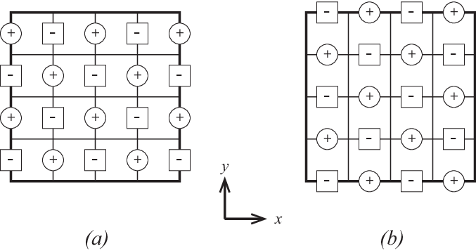
See Figure 4.1 (a)(a) for an illustration for ψx\psi_{x}. Notice that ψx\psi_{x} is well-defined whenever NxN_{x} is even. It is easy to see that ψx∉V#𝔅,h.\psi_{x}\not\in V^{\mathfrak{B},h}_{\#}. Similarly, we can find another piecewise linear function ψy\psi_{y} in V#h,V^{h}_{\#}, not belonging to V#𝔅,hV^{\mathfrak{B},h}_{\#} (Figure 4.1 (b)(b)), such that its midpoint values on topologically horizontal edges are ±1\pm 1 with alternating sign in both directions and all the midpoint values on topologically vertical edges are 0.
Refer to caption
Figure 4.1: An example of two alternating functions (a)(a) ψx\psi_{x} and (b)(b) ψy\psi_{y}. They do not belong to 𝔅\mathfrak{B}.

Next, let us consider the case where either NxN_{x} or NyN_{y} is odd. Propositions 7 and  8 imply that 𝔅\mathfrak{B} is linearly independent and dim⁡V#𝔅,h=dim⁡V#h.\operatorname{dim}\,V^{\mathfrak{B},h}_{\#}=\operatorname{dim}\,V^{h}_{\#}. Therefore V#𝔅,h=V#hV^{\mathfrak{B},h}_{\#}=V^{h}_{\#} and 𝔅\mathfrak{B}, the set of all node–based functions, is a basis for V#hV^{h}_{\#}. We summarize these results as in following theorem.

Theorem 9.

(A basis for V#hV^{h}_{\#})

  1. 1.

    If both NxN_{x} and NyN_{y} are even, then V#𝔅,h⫋V#hV^{\mathfrak{B},h}_{\#}\subsetneqq V^{h}_{\#}. Furthermore 𝔄={ψx,ψy}\mathfrak{A}=\{\psi_{x},\psi_{y}\} where ψx\psi_{x} and ψy\psi_{y} are defined as in (4.2), forms a complementary basis for V#h,V^{h}_{\#}, not belonging to V#𝔅,hV^{\mathfrak{B},h}_{\#}. Moreover, 𝔅♭∪𝔄\mathfrak{B}^{\flat}\cup\mathfrak{A} forms a basis for V#h,V^{h}_{\#}, where 𝔅♭={ϕ1,⋯,ϕ|𝔅|−1}\mathfrak{B}^{\flat}=\{\phi_{1},\cdots,\phi_{|\mathfrak{B}|-1}\}.

  2. 2.

    If either NxN_{x} or NyN_{y} is odd, then V#𝔅,h=V#hV^{\mathfrak{B},h}_{\#}=V^{h}_{\#}. Moreover, 𝔅\mathfrak{B} is a basis for V#hV^{h}_{\#}.

Remark 10.

Notice that the elementwise derivatives ∂ψx∂x\frac{\partial\psi_{x}}{\partial x} and ∂ψy∂y\frac{\partial\psi_{y}}{\partial y} are checkerboard patterns, while ∂ψx∂y=∂ψy∂x=0.\frac{\partial\psi_{x}}{\partial y}=\frac{\partial\psi_{y}}{\partial x}=0.

4.3 Stiffness matrix associated with 𝔅\mathfrak{B}

Even though 𝔅\mathfrak{B} may not be a basis for V#hV^{h}_{\#}, it is still a useful set of functions to understand V#hV^{h}_{\#}. Above all, the node–based functions are easy to handle in implementation viewpoint. Furthermore, Theorem 9 implies V#𝔅,h,V^{\mathfrak{B},h}_{\#}, which equals to Span⁡(𝔅)\operatorname{Span}(\mathfrak{B}), occupies almost all of V#h.V^{h}_{\#}. In this section, we investigate some characteristics of 𝔅\mathfrak{B} in approximating the Laplace operator.

Refer to caption
Figure 4.2: The stencil for 𝐒h𝔅\mathbf{S}^{\mathfrak{B}}_{h} with uniform cubes of size h×hh\times h.

Set 𝐒h𝔅\mathbf{S}^{\mathfrak{B}}_{h} be the |𝔅|×|𝔅||\mathfrak{B}|\times|\mathfrak{B}| stiffness matrix associated with 𝔅={ϕj}j=1|𝔅|,\mathfrak{B}=\{\phi_{j}\}_{j=1}^{|\mathfrak{B}|}, whose components are given by

(4.5) (𝐒h𝔅)j​k=∑K∈𝒯h∫K∇ϕk⋅∇ϕj1≤j,k≤|𝔅|.\displaystyle(\mathbf{S}^{\mathfrak{B}}_{h})_{jk}=\sum_{K\in{\mathcal{T}}_{h}}\int_{K}\nabla\phi_{k}\cdot\nabla\phi_{j}\quad 1\leq j,k\leq|\mathfrak{B}|.

The local stencil for the stiffness matrix associated with 𝔅\mathfrak{B} is shown in Figure 4.2. Obviously, 𝐒h𝔅\mathbf{S}^{\mathfrak{B}}_{h} is symmetric and positive semi-definite. The following lemma and proposition are immediate, but useful for later uses.

Lemma 11.

Let vh=∑jvj​ϕjv_{h}=\sum_{j}v_{j}\phi_{j} for 𝐯=(vj)∈ℝ|𝔅|\mathbf{v}=(v_{j})\in\mathbb{R}^{|\mathfrak{B}|}. Then 𝐯∈ker⁡𝐒h𝔅\mathbf{v}\in\ker\mathbf{S}^{\mathfrak{B}}_{h} if and only if vhv_{h} is a constant function in Ω\Omega.

Proposition 12.

ker⁡𝐒h𝔅\ker\mathbf{S}^{\mathfrak{B}}_{h} can be decomposed as

(4.6) ker⁡𝐒h𝔅=ker⁡Bh𝔅⊕Span⁡𝟏𝔅.\displaystyle\ker\mathbf{S}^{\mathfrak{B}}_{h}=\ker B^{\mathfrak{B}}_{h}\oplus\operatorname{Span}\mathbf{1}_{\mathfrak{B}}.

Remark 13.

Lemma 11 and Proposition 12 are also valid in the 3D case.

Observe that Propositions 8 and  12 directly lead to the following proposition.

Proposition 14.

(The dimension of ker⁡𝐒h𝔅\ker\mathbf{S}^{\mathfrak{B}}_{h})

(4.7) dim⁡ker⁡𝐒h𝔅=𝔢⁡(Nx)​𝔢​(Ny)+1.\displaystyle\operatorname{dim}\,\ker\mathbf{S}^{\mathfrak{B}}_{h}=\mathfrak{e}(N_{x})\mathfrak{e}(N_{y})+1.

5 Numerical Schemes for Elliptic Problems with Periodic BC

Assume that f∈L2​(Ω)f\in L^{2}(\Omega) is given such that ∫Ωf=0.\int_{\Omega}f=0. Consider the elliptic problem with periodic BC to find u∈H#1​(Ω)/ℝu\in H^{1}_{\#}(\Omega)/{\mathbb{R}} such that −Δ​u=f​in ​Ω.-\Delta u=f\ \text{in }\Omega. The weak formulation is as follows: find u∈H#1​(Ω)/ℝu\in H^{1}_{\#}(\Omega)/{\mathbb{R}} such that

(5.1) ∫Ω∇u⋅∇v=∫Ωf​v∀v∈H#1​(Ω)/ℝ.\int_{\Omega}\nabla u\cdot\nabla v=\int_{\Omega}fv\quad\,\forall v\in H^{1}_{\#}(\Omega)/{\mathbb{R}}.

By defining ah​(uh,vh):=∑K∈𝒯h∫K∇uh⋅∇vha_{h}(u_{h},v_{h}):=\sum_{K\in{\mathcal{T}}_{h}}\int_{K}\nabla u_{h}\cdot\nabla v_{h}, the discrete weak formulation for (5.1) is given as follows: find uh∈V#h/ℝu_{h}\in V^{h}_{\#}/{\mathbb{R}} such that

(5.2) ah​(uh,vh)=∫Ωf​vh∀vh∈V#h/ℝ.a_{h}(u_{h},v_{h})=\int_{\Omega}fv_{h}\quad\,\forall v_{h}\in V^{h}_{\#}/{\mathbb{R}}.
Remark 15.

Throughout this section, we assume that both NxN_{x} and NyN_{y} are even. The other cases with odd NxN_{x} and/or NyN_{y} are easy to handle owing to V#h=V#𝔅,hV^{h}_{\#}=V^{\mathfrak{B},h}_{\#}. Also we will assume that (𝒯h)0<h({\mathcal{T}}_{h})_{0<h} is a family of uniform rectangular decomposition.

Additional Notations & Properties

We compare 4 different numerical approaches to solve (5.2) with the trial and test function spaces 𝒮=𝔅♭,𝔅,𝔈♭,𝔈,\mathcal{S}=\mathfrak{B}^{\flat},\mathfrak{B},\mathfrak{E}^{\flat},\mathfrak{E}, which are described as follows. Due to Proposition 8, we can find 𝔅♭\mathfrak{B}^{\flat}, a proper subset of 𝔅\mathfrak{B}, which is a basis for V#𝔅,hV^{\mathfrak{B},h}_{\#}. It clearly holds that |𝔅♭|=dim⁡V#𝔅,h=|𝔅|−1|\mathfrak{B}^{\flat}|=\operatorname{dim}\,V^{\mathfrak{B},h}_{\#}=|\mathfrak{B}|-1. Consider the two extended sets 𝔈:=𝔅∪𝔄\mathfrak{E}:=\mathfrak{B}\cup\mathfrak{A} and 𝔈♭:=𝔅♭∪𝔄,\mathfrak{E}^{\flat}:=\mathfrak{B}^{\flat}\cup\mathfrak{A}, the latter of which is a basis for V#hV^{h}_{\#}. The characteristics of 𝔅♭\mathfrak{B}^{\flat}, 𝔅\mathfrak{B}, 𝔈♭\mathfrak{E}^{\flat}, and 𝔈\mathfrak{E} are summarized in Table 5.1.

𝒮\mathcal{S} |𝒮||\mathcal{S}| Span⁡𝒮\operatorname{Span}\mathcal{S} dim⁡Span⁡𝒮\operatorname{dim}\,\operatorname{Span}\mathcal{S}
𝔅♭\mathfrak{B}^{\flat} Nx​Ny−1N_{x}N_{y}-1 V#𝔅,hV^{\mathfrak{B},h}_{\#} Nx​Ny−1N_{x}N_{y}-1
𝔅\mathfrak{B} Nx​NyN_{x}N_{y}
𝔈♭\mathfrak{E}^{\flat} Nx​Ny+1N_{x}N_{y}+1 V#hV^{h}_{\#} Nx​Ny+1N_{x}N_{y}+1
𝔈\mathfrak{E} Nx​Ny+2N_{x}N_{y}+2
Table 5.1: Characteristics of each test and trial function set 𝒮\mathcal{S} when both NxN_{x}, NyN_{y} are even

For a vector 𝐯\mathbf{v} with |𝔈||\mathfrak{E}| (or |𝔈♭||\mathfrak{E}^{\flat}|) number of components, let 𝐯|𝔅\mathbf{v}|_{\mathfrak{B}} (or 𝐯|𝔅♭\mathbf{v}|_{\mathfrak{B}^{\flat}}) and 𝐯|𝔄\mathbf{v}|_{\mathfrak{A}} denote vectors consisting of the first |𝔅||\mathfrak{B}| (or |𝔅♭||\mathfrak{B}^{\flat}|) components, and of the last |𝔄||\mathfrak{A}| components, respectively. Several properties of functions in 𝔅\mathfrak{B} and 𝔄\mathfrak{A} can be observed.

Lemma 16.

Let 𝔅\mathfrak{B} and 𝔄\mathfrak{A} be as above. Then the followings hold.

  1. 1.

    ah​(ϕ,ψ)=0​∀ϕ∈𝔅​∀ψ∈𝔄a_{h}(\phi,\psi)=0\,\forall\phi\in\mathfrak{B}\,\forall\psi\in\mathfrak{A}.

  2. 2.

    ah​(ψμ,ψν)=0​∀ψμ,ψν∈𝔄a_{h}(\psi_{\mu},\psi_{\nu})=0\,\forall\psi_{\mu},\psi_{\nu}\in\mathfrak{A} such that μ≠ν\mu\not=\nu.

  3. 3.

    ∫Ωψ=0​∀ψ∈𝔄\int_{\Omega}\psi=0\,\forall\psi\in\mathfrak{A}.

  4. 4.

    There exists an hh-independent constant CC such that ‖ψ‖0≤C\|\psi\|_{0}\leq C and |ψ|1,h≤C​h−1​∀ψ∈𝔄|\psi|_{1,h}\leq Ch^{-1}\,\forall\psi\in\mathfrak{A}.

Now, we define a stiffness matrix associated with 𝔅♭\mathfrak{B}^{\flat}, and its variants. Let 𝐒h𝔅♭\mathbf{S}^{\mathfrak{B}^{\flat}}_{h} be the |𝔅♭|×|𝔅♭||\mathfrak{B}^{\flat}|\times|\mathfrak{B}^{\flat}| stiffness matrix associated with 𝔅♭\mathfrak{B}^{\flat} whose components are given by

(5.3) (𝐒h𝔅♭)j​k:=ah​(ϕk,ϕj)1≤j,k≤|𝔅♭|,\displaystyle(\mathbf{S}^{\mathfrak{B}^{\flat}}_{h})_{jk}:=a_{h}(\phi_{k},\phi_{j})\quad 1\leq j,k\leq|\mathfrak{B}^{\flat}|,

and 𝐒~h𝔅♭\mathbf{\tilde{S}}^{\mathfrak{B}^{\flat}}_{h} be the same matrix as 𝐒h𝔅♭\mathbf{S}^{\mathfrak{B}^{\flat}}_{h}, but the last row is modified in order to impose the zero mean value condition. Because all the integrals ∫Ωϕj\int_{\Omega}\phi_{j} are same for all ϕj\phi_{j} in 𝔅\mathfrak{B}, every entry in the last row is replaced by 11.

(5.4) (𝐒~h𝔅♭)j​k:={ah​(ϕk,ϕj)j≠|𝔅♭|,1j=|𝔅♭|.\displaystyle(\mathbf{\tilde{S}}^{\mathfrak{B}^{\flat}}_{h})_{jk}:=\begin{cases}a_{h}(\phi_{k},\phi_{j})&j\not=|\mathfrak{B}^{\flat}|,\\ 1&j=|\mathfrak{B}^{\flat}|.\end{cases}

Note that 𝐒~h𝔅♭\mathbf{\tilde{S}}^{\mathfrak{B}^{\flat}}_{h} is nonsingular whereas both 𝐒h𝔅\mathbf{S}^{\mathfrak{B}}_{h} and 𝐒h𝔅♭\mathbf{S}^{\mathfrak{B}^{\flat}}_{h} are singular with rank deficiency 22 and 11, respectively. For the complementary part, let 𝐒h𝔄\mathbf{S}^{\mathfrak{A}}_{h} be the |𝔄|×|𝔄||\mathfrak{A}|\times|\mathfrak{A}| stiffness matrix associated with 𝔄\mathfrak{A},

(5.5) (𝐒h𝔄)j​k:=ah​(ψk,ψj)1≤j,k≤|𝔄|.\displaystyle(\mathbf{S}^{\mathfrak{A}}_{h})_{jk}:=a_{h}(\psi_{k},\psi_{j})\quad 1\leq j,k\leq|\mathfrak{A}|.

Notice that 𝐒h𝔄\mathbf{S}^{\mathfrak{A}}_{h} is a nonsingular diagonal matrix due to Lemma 16.

5.1 Option 1: 𝒮=𝔈♭\mathcal{S}=\mathfrak{E}^{\flat} for a nonsingular nonsymmetric system

Since 𝔈♭\mathfrak{E}^{\flat} is a basis for V#hV^{h}_{\#}, 𝔈♭\mathfrak{E}^{\flat} is a natural choice as a set of trial and test functions to assemble a linear system corresponding to (5.2). The numerical solution uh∈V#hu_{h}\in V^{h}_{\#} is uniquely expressed, associated with 𝔈♭\mathfrak{E}^{\flat}, as

(5.6) uh=𝐮~♭​𝔈♭\displaystyle u_{h}=\mathbf{\tilde{u}^{\flat}}\mathfrak{E}^{\flat}

where 𝐮~♭\mathbf{\tilde{u}^{\flat}} is the solution of the following system of equations associated with 𝔈♭\mathfrak{E}^{\flat}:

(5.7) ℒ~h𝔈♭​𝐮~♭=[𝐟~𝔅♭𝐟𝔄]\mathcal{\tilde{L}}^{\mathfrak{E}^{\flat}}_{h}\mathbf{\tilde{u}^{\flat}}=\begin{bmatrix}\mathbf{\tilde{f}}_{\mathfrak{B}^{\flat}}\\ \mathbf{f}_{\mathfrak{A}}\end{bmatrix}

where ℒ~h𝔈♭:=[𝐒~h𝔅♭𝟎𝟎𝐒h𝔄],\mathcal{\tilde{L}}^{\mathfrak{E}^{\flat}}_{h}:=\begin{bmatrix}\mathbf{\tilde{S}}^{\mathfrak{B}^{\flat}}_{h}&\mathbf{0}\\ \mathbf{0}&\mathbf{S}^{\mathfrak{A}}_{h}\end{bmatrix}, (𝐟~𝔅♭)j={∫Ωf​ϕj,1≤j<|𝔅♭|0,j=|𝔅♭|,(\mathbf{\tilde{f}}_{\mathfrak{B}^{\flat}})_{j}=\begin{cases}\int_{\Omega}f\phi_{j},&1\leq j<|\mathfrak{B}^{\flat}|\\ 0,&j=|\mathfrak{B}^{\flat}|\end{cases}, and 𝐟𝔄=∫Ωf​𝔄.\mathbf{f}_{\mathfrak{A}}=\int_{\Omega}f\mathfrak{A}. Due to Lemma 16, ℒ~h𝔈♭\mathcal{\tilde{L}}^{\mathfrak{E}^{\flat}}_{h} is a block-diagonal matrix. Moreover, it is nonsingular, but nonsymmetric due to the modification in the last row of 𝐒~𝔅♭\mathbf{\tilde{S}}^{\mathfrak{B}^{\flat}} which comes from the zero mean value condition. We can use any known numerical scheme for general linear systems, for instance GMRES, to solve (5.7).

Scheme 1.

GMRES for 𝒮=𝔈♭\mathcal{S}=\mathfrak{E}^{\flat}
Step 1. Take an initial vector 𝐮(0)∈ℝ|𝔈♭|.\mathbf{u}^{(0)}\in\mathbb{R}^{|\mathfrak{E}^{\flat}|}.
Step 2. Solve the nonsymmetric system (5.7) by a restarted GMRES and set 𝐮~♭:=𝐮(n)\mathbf{\tilde{u}^{\flat}}:=\mathbf{u}^{(n)}.
Step 3. The numerical solution is obtained as uh=𝐮~♭​𝔈♭u_{h}=\mathbf{\tilde{u}^{\flat}}\mathfrak{E}^{\flat}.

5.2 Option 2: 𝒮=𝔈♭\mathcal{S}=\mathfrak{E}^{\flat} for a symmetric positive semi-definite system with rank deficiency 1

In the previous approach, the zero mean value condition is imposed in a system of equations directly. Consequently the associated linear system becomes nonsymmetric due to modification of just a single row.

In this subsection we will impose the zero mean value condition indirectly in order to conserve symmetry of the assembled linear system. In particular, we will impose the zero mean value condition in post-processing stage. Then we can apply some fast solvers for symmetric system. On the other hand, nonsingularity can not be avoided any longer in this approach. Fortunately the linear system is at least positive semi-definite. Hence we can use a Drazin inverse as mentioned in Section 2.1 to solve our singular system using a Krylov iterative method under a proper condition.

Consider a system of equations for (5.2) associated with 𝔈♭\mathfrak{E}^{\flat} without any modification:

(5.8) ℒh𝔈♭​𝐮♭=∫Ωf​𝔈♭whereℒh𝔈♭:=[𝐒h𝔅♭𝟎𝟎𝐒h𝔄].\displaystyle\mathcal{L}^{\mathfrak{E}^{\flat}}_{h}\mathbf{u^{\flat}}=\int_{\Omega}f\mathfrak{E}^{\flat}\quad\text{where}\quad\mathcal{L}^{\mathfrak{E}^{\flat}}_{h}:=\begin{bmatrix}\mathbf{S}^{\mathfrak{B}^{\flat}}_{h}&\mathbf{0}\\ \mathbf{0}&\mathbf{S}^{\mathfrak{A}}_{h}\end{bmatrix}.

Note that the above linear system is singular, and symmetric positive semi-definite. We should find the solution 𝐮♭\mathbf{u^{\flat}} of the system such that

(5.9) 𝐮♭|𝔅♭⋅𝟏𝔅♭=0\displaystyle\mathbf{u^{\flat}}|_{\mathfrak{B}^{\flat}}\cdot\mathbf{1}_{\mathfrak{B}^{\flat}}=0

since ∫Ω𝐯​𝔈♭=0\int_{\Omega}\mathbf{v}\mathfrak{E}^{\flat}=0 if and only if 𝐯|𝔅♭⋅𝟏𝔅♭=0\mathbf{v}|_{\mathfrak{B}^{\flat}}\cdot\mathbf{1}_{\mathfrak{B}^{\flat}}=0, and the numerical solution uh♭∈V#hu^{\flat}_{h}\in V^{h}_{\#} of this scheme is obtained by

(5.10) uh♭=𝐮♭​𝔈♭.\displaystyle u^{\flat}_{h}=\mathbf{u^{\flat}}\mathfrak{E}^{\flat}.

If a symmetric positive semi-definite system A​x=bAx=b is given, as our formulation above, the conjugate gradient method (CG) gives a unique Krylov solution if the consistency condition b∈Im⁡Ab\in\operatorname{Im}A holds. The general solution is obviously obtained upto its kernel. The kernel of the linear system (5.8) is closely related with the kernel of 𝐒h𝔅♭\mathbf{S}^{\mathfrak{B}^{\flat}}_{h}. A simple analog of Section 4.3 implies that the dimension of ker⁡𝐒h𝔅♭\ker\mathbf{S}^{\mathfrak{B}^{\flat}}_{h} is 11, and 𝐯∈ker⁡𝐒h𝔅♭\mathbf{v}\in\ker\mathbf{S}^{\mathfrak{B}^{\flat}}_{h} if and only if 𝐯​𝔅♭\mathbf{v}\mathfrak{B}^{\flat} is a constant function in Ω\Omega. Note that 𝔅♭\mathfrak{B}^{\flat} is not a partition of unity, whereas 𝔅\mathfrak{B} is. Let 𝐰𝔅♭\mathbf{w}_{\mathfrak{B}^{\flat}} denote a unique vector in ℝ|𝔅♭|\mathbb{R}^{|\mathfrak{B}^{\flat}|} such that 𝐰𝔅♭​𝔅♭≡1\mathbf{w}_{\mathfrak{B}^{\flat}}\mathfrak{B}^{\flat}\equiv 1 in Ω\Omega. Then the kernel of the linear system in (5.8) is simply represented by Span⁡𝐰𝔈♭\operatorname{Span}\mathbf{w}_{\mathfrak{E}^{\flat}} where

𝐰𝔈♭=[𝐰𝔅♭T𝟎]T∈ℝ|𝔈♭|\mathbf{w}_{\mathfrak{E}^{\flat}}=\begin{bmatrix}\mathbf{w}_{\mathfrak{B}^{\flat}}^{T}&\mathbf{0}\end{bmatrix}^{T}\in\mathbb{R}^{|\mathfrak{E}^{\flat}|}

is the trivial extension of 𝐰𝔅♭.\mathbf{w}_{\mathfrak{B}^{\flat}}. Therefore in the post-processing stage we add a multiple of 𝐰𝔈♭\mathbf{w}_{\mathfrak{E}^{\flat}} to the Krylov solution to preserve (5.9).

In summary, the numerical scheme for uh♭u^{\flat}_{h} is given as follows.

Scheme 2.

CG for 𝒮=𝔈♭\mathcal{S}=\mathfrak{E}^{\flat} of rank 1 deficiency
Step 1. Take a vector 𝐮(0)∈ℝ|𝔈♭|\mathbf{u}^{(0)}\in\mathbb{R}^{|\mathfrak{E}^{\flat}|} for an initial guess.
Step 2. Solve the singular symmetric positive semi-definite system (5.8) by the CG and get the Krylov solution 𝐮′=𝐮(n)\mathbf{u^{\prime}}=\mathbf{u}^{(n)}.
Step 3. Add a multiple of 𝐰𝔈♭\mathbf{w}_{\mathfrak{E}^{\flat}} to 𝐮′\mathbf{u^{\prime}} to get 𝐮♭\mathbf{u^{\flat}}, in order to enforce (5.9), as

𝐮♭=𝐮′−𝐮′|𝔅♭⋅𝟏𝔅♭𝐰𝔅♭⋅𝟏𝔅♭​𝐰𝔈♭.\displaystyle\mathbf{u^{\flat}}=\mathbf{u^{\prime}}-\frac{\mathbf{u^{\prime}}|_{\mathfrak{B}^{\flat}}\cdot\mathbf{1}_{\mathfrak{B}^{\flat}}}{\mathbf{w}_{\mathfrak{B}^{\flat}}\cdot\mathbf{1}_{\mathfrak{B}^{\flat}}}\mathbf{w}_{\mathfrak{E}^{\flat}}.

Step 4. The numerical solution is obtained as uh♭=𝐮♭​𝔈♭u^{\flat}_{h}=\mathbf{u^{\flat}}\mathfrak{E}^{\flat}.

5.3 Option 3: 𝒮=𝔈\mathcal{S}=\mathfrak{E} for a symmetric positive semi-definite system with rank deficiency 2

Although symmetry and positive semi-definiteness are key factors for an efficient numerical scheme for linear solvers, we may not enjoy full benefits in the previous scheme. We need the extra post-processing stage to impose the zero mean value condition. The defect in the previous approach comes from the fact that the Riesz representation vector for the integral functional does not belong to the kernel of the linear system. As shown above, the kernel of the linear system is closely related with the coefficient vector for the unity function. If these two vectors coincide, we can get our solution without any post-processing stage. The imbalance of 𝔅♭\mathfrak{B}^{\flat} for the linear independence is also a disadvantage to numerical implementation.

In this approach, we find the numerical solution uh♮∈V#hu^{\natural}_{h}\in V^{h}_{\#} such that

(5.11) uh♮=𝐮♮​𝔈\displaystyle u^{\natural}_{h}=\mathbf{u^{\natural}}\mathfrak{E}

where 𝐮♮\mathbf{u^{\natural}} is a solution of a system of equations for (5.2) associated with full 𝔈\mathfrak{E},

(5.12) ℒh𝔈​𝐮♮:=[𝐒h𝔅𝟎𝟎𝐒h𝔄]​𝐮♮=∫Ωf​𝔈\displaystyle\mathcal{L}^{\mathfrak{E}}_{h}\mathbf{u^{\natural}}:=\begin{bmatrix}\mathbf{S}^{\mathfrak{B}}_{h}&\mathbf{0}\\ \mathbf{0}&\mathbf{S}^{\mathfrak{A}}_{h}\end{bmatrix}\mathbf{u^{\natural}}=\int_{\Omega}f\mathfrak{E}

with

(5.13) 𝐮♮|𝔅⋅𝟏𝔅=0,\displaystyle\mathbf{u^{\natural}}|_{\mathfrak{B}}\cdot\mathbf{1}_{\mathfrak{B}}=0,

since ∫Ω𝐯​𝔈=0\int_{\Omega}\mathbf{v}\mathfrak{E}=0 if and only if 𝐯|𝔅⋅𝟏𝔅=0\mathbf{v}|_{\mathfrak{B}}\cdot\mathbf{1}_{\mathfrak{B}}=0. The numerical solution u♮u^{\natural} is unique because a solution of the linear system is unique upto an additive nontrivial representation for the zero function in 𝔅\mathfrak{B}. We want to emphasize that, unlike the previous scheme, 𝟏𝔅\mathbf{1}_{\mathfrak{B}} belongs to the kernel of 𝐒h𝔅\mathbf{S}^{\mathfrak{B}}_{h} as shown in (12). It implies that, without any extra post-processing stage, we can find the solution of the linear system which satisfies the zero mean value condition (5.13) if an initial guess is chosen to satisfy the same condition.

In summary, we have the numerical solution uh♮u^{\natural}_{h} as follows.

Scheme 3.

CG for 𝒮=𝔈\mathcal{S}=\mathfrak{E} of rank 2 deficiency
Step 1. Take an initial vector 𝐮(0)∈ℝ|𝔈|\mathbf{u}^{(0)}\in\mathbb{R}^{|\mathfrak{E}|} which satisfies 𝐮(0)|𝔅⋅𝟏𝔅=0\mathbf{u}^{(0)}|_{\mathfrak{B}}\cdot\mathbf{1}_{\mathfrak{B}}=0.
Step 2. Solve the singular symmetric positive semi-definite system (5.12) by the CG and get the Krylov solution 𝐮♮=𝐮(n)\mathbf{u^{\natural}}=\mathbf{u}^{(n)}.
Step 3. The numerical solution is obtained as uh♮=𝐮♮​𝔈u^{\natural}_{h}=\mathbf{u^{\natural}}\mathfrak{E}.

5.4 Option 4: 𝒮=𝔅\mathcal{S}=\mathfrak{B} for a symmetric positive semi-definite system with rank deficiency 2

Consider a system of equations associated only with 𝔅\mathfrak{B} for (5.2) to find 𝐮¯♮∈V#𝔅,h\mathbf{\bar{u}^{\natural}}\in V^{\mathfrak{B},h}_{\#} such that

(5.14) ℒh𝔅​𝐮¯♮:=𝐒h𝔅​𝐮¯♮=∫Ωf​𝔅.\displaystyle\mathcal{L}^{\mathfrak{B}}_{h}\mathbf{\bar{u}^{\natural}}:=\mathbf{S}^{\mathfrak{B}}_{h}\mathbf{\bar{u}^{\natural}}=\int_{\Omega}f\mathfrak{B}.

Starting from an initial vector 𝐮(0)∈ℝ|𝔅|\mathbf{u}^{(0)}\in\mathbb{R}^{|\mathfrak{B}|} which satisfies 𝐮(0)⋅𝟏𝔅=0\mathbf{u}^{(0)}\cdot\mathbf{1}_{\mathfrak{B}}=0, let 𝐮¯♮\mathbf{\bar{u}^{\natural}} be the Krylov solution of the linear system. The numerical solution u¯h♮∈V#𝔅,h\bar{u}^{\natural}_{h}\in V^{\mathfrak{B},h}_{\#} is obtained by

(5.15) u¯h♮=𝐮¯♮​𝔅.\displaystyle\bar{u}^{\natural}_{h}=\mathbf{\bar{u}^{\natural}}\mathfrak{B}.

We summarize the above procedure as follows.

Scheme 4.

CG for 𝒮=𝔅\mathcal{S}=\mathfrak{B} of rank 2 deficiency
Step 1. Take an initial vector 𝐮(0)∈ℝ|𝔈|\mathbf{u}^{(0)}\in\mathbb{R}^{|\mathfrak{E}|} which satisfies 𝐮(0)|𝔅⋅𝟏𝔅=0\mathbf{u}^{(0)}|_{\mathfrak{B}}\cdot\mathbf{1}_{\mathfrak{B}}=0.
Step 2. Solve the singular symmetric positive semi-definite system (5.14) by the CG and get the Krylov solution 𝐮¯♮=𝐮(n)\mathbf{\bar{u}^{\natural}}=\mathbf{u}^{(n)}.
Step 3. The numerical solution is obtained as u¯h♮=𝐮¯♮​𝔅\bar{u}^{\natural}_{h}=\mathbf{\bar{u}^{\natural}}\mathfrak{B}.

Main Theorem: Relation Between Numerical Solutions

The following theorem states the relation between all numerical solutions discussed above.

Theorem 17.

Let (𝒯h)0<h({\mathcal{T}}_{h})_{0<h} be a family of uniform rectangular decomposition, that is, 𝒯h=𝒯~h{\mathcal{T}}_{h}=\widetilde{\mathcal{T}}_{h} for all h.h. Assume that NxN_{x} and NyN_{y} are even. Let uhu_{h}, uh♭u^{\flat}_{h}, uh♮u^{\natural}_{h}, u¯h♮\bar{u}^{\natural}_{h} be the numerical solutions of (5.1) as (5.6), (5.10), (5.11), (5.15), respectively. Then uh=uh♭=uh♮u_{h}=u^{\flat}_{h}=u^{\natural}_{h}, and

‖uh♮−u¯h♮‖0≤C​h2​‖f‖0,|uh♮−u¯h♮|1,h≤C​h​‖f‖0.\|u^{\natural}_{h}-\bar{u}^{\natural}_{h}\|_{0}\leq Ch^{2}\|f\|_{0},\ |u^{\natural}_{h}-\bar{u}^{\natural}_{h}|_{1,h}\leq Ch\|f\|_{0}.

Remark 18.

Theorem 17 provides theoretical error bounds with a set of test and trial functions which are redundant but easy to implement, instead of a set of exact solutions which are exactly fitted but complicated to implement.

Proof.

Let 𝐮♭\mathbf{u^{\flat}} and 𝐮~♭\mathbf{\tilde{u}^{\flat}} be the solutions as in Sections 5.1 and 5.2, respectively. Note that two linear systems (5.7) and (5.8) coincide except |𝔅♭||\mathfrak{B}^{\flat}|-th row. Even on |𝔅♭||\mathfrak{B}^{\flat}|-th row,

(ℒ~h𝔈♭​𝐮♭)|𝔅♭|\displaystyle\left(\mathcal{\tilde{L}}^{\mathfrak{E}^{\flat}}_{h}\mathbf{u^{\flat}}\right)_{|\mathfrak{B}^{\flat}|} =𝟏𝔅♭⋅(𝐮′−𝐮′|𝔅♭⋅𝟏𝔅♭𝐰𝔅♭⋅𝟏𝔅♭​𝐰𝔈♭)|𝔅♭\displaystyle=\mathbf{1}_{\mathfrak{B}^{\flat}}\cdot\left.\left(\mathbf{u^{\prime}}-\frac{\mathbf{u^{\prime}}|_{\mathfrak{B}^{\flat}}\cdot\mathbf{1}_{\mathfrak{B}^{\flat}}}{\mathbf{w}_{\mathfrak{B}^{\flat}}\cdot\mathbf{1}_{\mathfrak{B}^{\flat}}}\mathbf{w}_{\mathfrak{E}^{\flat}}\right)\right|_{\mathfrak{B}^{\flat}}
=𝟏𝔅♭⋅(𝐮′|𝔅♭−𝐮′|𝔅♭⋅𝟏𝔅♭𝐰𝔅♭⋅𝟏𝔅♭​𝐰𝔅♭)\displaystyle=\mathbf{1}_{\mathfrak{B}^{\flat}}\cdot\left(\mathbf{u^{\prime}}|_{\mathfrak{B}^{\flat}}-\frac{\mathbf{u^{\prime}}|_{\mathfrak{B}^{\flat}}\cdot\mathbf{1}_{\mathfrak{B}^{\flat}}}{\mathbf{w}_{\mathfrak{B}^{\flat}}\cdot\mathbf{1}_{\mathfrak{B}^{\flat}}}\mathbf{w}_{\mathfrak{B}^{\flat}}\right)
=0.\displaystyle=0.

Thus ℒ~h𝔈♭​𝐮♭=[𝐟~𝔅♭𝐟𝔄]=ℒ~h𝔈♭​𝐮~♭\mathcal{\tilde{L}}^{\mathfrak{E}^{\flat}}_{h}\mathbf{u^{\flat}}=\begin{bmatrix}\mathbf{\tilde{f}}_{\mathfrak{B}^{\flat}}\\ \mathbf{f}_{\mathfrak{A}}\end{bmatrix}=\mathcal{\tilde{L}}^{\mathfrak{E}^{\flat}}_{h}\mathbf{\tilde{u}^{\flat}}, and it implies 𝐮♭=𝐮~♭\mathbf{u^{\flat}}=\mathbf{\tilde{u}^{\flat}} because ℒ~h𝔈♭\mathcal{\tilde{L}}^{\mathfrak{E}^{\flat}}_{h} is nonsingular. It concludes uh=uh♭u_{h}=u^{\flat}_{h}.

Let 𝐮♮\mathbf{u^{\natural}} be the solution as in Section 5.3. Then, we have 𝐮♮|𝔄=𝐮♭|𝔄.\mathbf{u^{\natural}}|_{\mathfrak{A}}=\mathbf{u^{\flat}}|_{\mathfrak{A}}. Let [𝐮♭|𝔅♭0]\begin{bmatrix}\mathbf{u^{\flat}}|_{\mathfrak{B}^{\flat}}\\ 0\end{bmatrix} be a trivial extension of 𝐮♭|𝔅♭\mathbf{u^{\flat}}|_{\mathfrak{B}^{\flat}} into a vector in ℝ|𝔅|\mathbb{R}^{|\mathfrak{B}|} by padding a single zero. Note that ∑j=1|𝔅|(𝐒h𝔅)j​k=0\sum_{j=1}^{|\mathfrak{B}|}(\mathbf{S}^{\mathfrak{B}}_{h})_{jk}=0 for all 1≤k≤|𝔅|1\leq k\leq|\mathfrak{B}|. Due to the definition of 𝐮♭\mathbf{u^{\flat}}, we have

𝐒h𝔅​[𝐮♭|𝔅♭0]\displaystyle\mathbf{S}^{\mathfrak{B}}_{h}\begin{bmatrix}\mathbf{u^{\flat}}|_{\mathfrak{B}^{\flat}}\\ 0\end{bmatrix} =[𝐒h𝔅♭​𝐮♭|𝔅♭[𝐒𝔅h]|𝔅|,1:|𝔅♭|𝐮♭|𝔅♭]=[∫Ωf​𝔅♭−∑j≠|𝔅|[𝐒𝔅h]j,1:|𝔅♭|𝐮♭|𝔅♭]\displaystyle=\begin{bmatrix}\mathbf{S}^{\mathfrak{B}^{\flat}}_{h}\mathbf{u^{\flat}}|_{\mathfrak{B}^{\flat}}\\ [\mathbf{S}^{\mathfrak{B}}_{h}]_{|\mathfrak{B}|,1:|\mathfrak{B}^{\flat}|}\mathbf{u^{\flat}}|_{\mathfrak{B}^{\flat}}\end{bmatrix}=\begin{bmatrix}\int_{\Omega}f\mathfrak{B}^{\flat}\\ -\sum_{j\not=|\mathfrak{B}|}\limits[\mathbf{S}^{\mathfrak{B}}_{h}]_{j,1:|\mathfrak{B}^{\flat}|}\mathbf{u^{\flat}}|_{\mathfrak{B}^{\flat}}\end{bmatrix}
=[∫Ωf​𝔅♭−∑j=1|𝔅♭|[𝐒𝔅♭h]j,1:|𝔅♭|𝐮♭|𝔅♭]=[∫Ωf​𝔅♭−∑j=1|𝔅♭|∫Ωfϕj]\displaystyle=\begin{bmatrix}\int_{\Omega}f\mathfrak{B}^{\flat}\\ -\sum_{j=1}^{|\mathfrak{B}^{\flat}|}[\mathbf{S}^{\mathfrak{B}^{\flat}}_{h}]_{j,1:|\mathfrak{B}^{\flat}|}\mathbf{u^{\flat}}|_{\mathfrak{B}^{\flat}}\end{bmatrix}=\begin{bmatrix}\int_{\Omega}f\mathfrak{B}^{\flat}\\ -\sum_{j=1}^{|\mathfrak{B}^{\flat}|}\int_{\Omega}f\phi_{j}\end{bmatrix}
=[∫Ωf​𝔅♭∫Ωf⁡(ϕ|𝔅|−1)]=∫Ωf​𝔅,\displaystyle=\begin{bmatrix}\int_{\Omega}f\mathfrak{B}^{\flat}\\ \int_{\Omega}f(\phi_{|\mathfrak{B}|}-1)\end{bmatrix}=\int_{\Omega}f\mathfrak{B},

since 𝔅\mathfrak{B} is a partition of unity and ∫Ωf=0\int_{\Omega}f=0. On the other hand, the definition of 𝐮♮\mathbf{u^{\natural}} implies 𝐒h𝔅​𝐮♮|𝔅=∫Ωf​𝔅\mathbf{S}^{\mathfrak{B}}_{h}\mathbf{u^{\natural}}|_{\mathfrak{B}}=\int_{\Omega}f\mathfrak{B}. Thus 𝐮♮|𝔅−[𝐮♭|𝔅♭0]\mathbf{u^{\natural}}|_{\mathfrak{B}}-\begin{bmatrix}\mathbf{u^{\flat}}|_{\mathfrak{B}^{\flat}}\\ 0\end{bmatrix} is in the kernel of 𝐒h𝔅\mathbf{S}^{\mathfrak{B}}_{h}, which is decomposed as Proposition 12. Due to the zero mean value condition in each scheme, (𝐮♮|𝔅−[𝐮♭|𝔅♭0])⋅𝟏𝔅=𝐮♮|𝔅⋅𝟏𝔅−𝐮♭|𝔅♭⋅𝟏𝔅♭=0\left(\mathbf{u^{\natural}}|_{\mathfrak{B}}-\begin{bmatrix}\mathbf{u^{\flat}}|_{\mathfrak{B}^{\flat}}\\ 0\end{bmatrix}\right)\cdot\mathbf{1}_{\mathfrak{B}}=\mathbf{u^{\natural}}|_{\mathfrak{B}}\cdot\mathbf{1}_{\mathfrak{B}}-\mathbf{u^{\flat}}|_{\mathfrak{B}^{\flat}}\cdot\mathbf{1}_{\mathfrak{B}^{\flat}}=0. Therefore 𝐮♮|𝔅−[𝐮♭|𝔅♭0]\mathbf{u^{\natural}}|_{\mathfrak{B}}-\begin{bmatrix}\mathbf{u^{\flat}}|_{\mathfrak{B}^{\flat}}\\ 0\end{bmatrix} must belong to ker⁡Bh𝔅\ker B^{\mathfrak{B}}_{h}, and consequently (𝐮♮|𝔅−[𝐮♭|𝔅♭0])​𝔅=𝐮♮|𝔅​𝔅−𝐮♭|𝔅♭​𝔅♭\left(\mathbf{u^{\natural}}|_{\mathfrak{B}}-\begin{bmatrix}\mathbf{u^{\flat}}|_{\mathfrak{B}^{\flat}}\\ 0\end{bmatrix}\right)\mathfrak{B}=\mathbf{u^{\natural}}|_{\mathfrak{B}}\mathfrak{B}-\mathbf{u^{\flat}}|_{\mathfrak{B}^{\flat}}\mathfrak{B}^{\flat} is equal to 00. This implies uh♮=uh♭u^{\natural}_{h}=u^{\flat}_{h}.

Let 𝐮¯♮\mathbf{\bar{u}^{\natural}} be the solution as in Section 5.4. Note that 𝐮♮|𝔅=𝐮¯♮\mathbf{u^{\natural}}|_{\mathfrak{B}}=\mathbf{\bar{u}^{\natural}}, and

𝐮♮|𝔄=diag⁡(ah​(ψx,ψx),ah​(ψy,ψy))−1​∫Ωf​𝔄≤C​h2​∫Ωf​𝔄\displaystyle\mathbf{u^{\natural}}|_{\mathfrak{A}}=\operatorname{diag}\left(a_{h}(\psi_{x},\psi_{x}),a_{h}(\psi_{y},\psi_{y})\right)^{-1}\int_{\Omega}f\mathfrak{A}\leq Ch^{2}\int_{\Omega}f\mathfrak{A}

due to Lemma 16. Owing to ∫Ωf​ψ≤C​(∫Ω|f|2)1/2​(∫Ω|ψ|2)1/2≤C​‖f‖0​∀ψ∈𝔄,\int_{\Omega}f\psi\leq C\left(\int_{\Omega}|f|^{2}\right)^{1/2}\left(\int_{\Omega}|\psi|^{2}\right)^{1/2}\leq C\|f\|_{0}\,\forall\psi\in\mathfrak{A}, each component of 𝐮♮|𝔄\mathbf{u^{\natural}}|_{\mathfrak{A}} is bounded by 𝒪⁡(h2)\mathcal{O}(h^{2}). Hence we have desired estimates the difference between uh♮u^{\natural}_{h} and u¯h♮\bar{u}^{\natural}_{h} in L2L^{2}- and H1H^{1}-(semi-)norm.

5.5 Numerical results

For the scheme Option 1, we use the restarted GMRES scheme in MGMRES library provided by Ju and Burkardt [21]. We emphasize that we replace one of essentially linearly dependent rows of 𝐒h𝔅♭\mathbf{S}^{\mathfrak{B}^{\flat}}_{h} by the zero mean value condition in order to make 𝐒~h𝔅♭\mathbf{\tilde{S}}^{\mathfrak{B}^{\flat}}_{h} nonsingular.

Example 19.

Consider the problem (5.1) on the domain Ω=(0,1)2\Omega=(0,1)^{2} with the exact solution u⁡(x,y)=s⁡(x)​s​(y)u(x,y)=s(x)s(y) where s⁡(t)=∑k=134(2​k−1)​π​sin⁡(2​(2​k−1)​π​t),s(t)=\sum_{k=1}^{3}\frac{4}{(2k-1)\pi}\sin\Big(2(2k-1)\pi t\Big), a truncated Fourier series for the square wave.

For each option, the error in energy norm and L2L^{2}-norm for Example 19 are shown in Table 5.2. We observe that all schemes give very similar numerical solutions.

Example 20.

Consider the same problem as in Example 19 with the exact solution u⁡(x,y)=s⁡(x)​s​(y)u(x,y)=s(x)s(y) where s⁡(t)=exp⁡(−11−(2​t−1)2)​t2​(1−t)+C,s(t)=\exp\left(-\frac{1}{1-(2t-1)^{2}}\right)t^{2}(1-t)+C, with a constant CC satisfying ∫[0,1]s=0\int_{[0,1]}s=0.

Table 5.3 shows numerical results for Example 20 in each option, and all options give almost the same result, as the previous example. The iteration number and elapsed time in each option in the case of h=1/256h=1/256 are shown in Table 5.4. We observe decrease of the iteration number and elapsed time in the option 3 compared to the option 2. Decrease from the option 3 to the option 4 is quite natural because we only use the node–based functions as trial and test functions for the option 4.

Opt 1 Opt 2
hh |u−uh|1,h|u-u_{h}|_{1,h} order ‖u−uh‖0\|u-u_{h}\|_{0} order |u−uh♭|1,h|u-u^{\flat}_{h}|_{1,h} order ‖u−uh♭‖0\|u-u^{\flat}_{h}\|_{0} order
1/8 1.123E+01 - 4.230E-01 - 1.123E+01 - 4.230E-01 -
1/16 5.466E-00 1.039 8.607E-02 2.297 5.466E-00 1.039 8.607E-02 2.297
1/32 2.832E-00 0.949 2.216E-02 1.957 2.832E-00 0.949 2.216E-02 1.957
1/64 1.429E-00 0.987 5.585E-03 1.989 1.429E-00 0.987 5.585E-03 1.989
1/128 7.160E-01 0.997 1.399E-03 1.997 7.160E-01 0.997 1.399E-03 1.997
1/256 3.582E-01 0.999 3.499E-04 1.999 3.582E-01 0.999 3.499E-04 1.999
Opt 3 Opt 4
hh |u−uh♮|1,h|u-u^{\natural}_{h}|_{1,h} order ‖u−uh♮‖0\|u-u^{\natural}_{h}\|_{0} order |u−u¯h♮|1,h|u-\bar{u}^{\natural}_{h}|_{1,h} order ‖u−u¯h♮‖0\|u-\bar{u}^{\natural}_{h}\|_{0} order
1/8 1.123E+01 - 4.230E-01 - 1.123E+01 - 4.230E-01 -
1/16 5.466E-00 1.039 8.607E-02 2.297 5.466E-00 1.039 8.607E-02 2.297
1/32 2.832E-00 0.949 2.216E-02 1.957 2.832E-00 0.949 2.216E-02 1.957
1/64 1.429E-00 0.987 5.585E-03 1.989 1.429E-00 0.987 5.585E-03 1.989
1/128 7.160E-01 0.997 1.399E-03 1.997 7.160E-01 0.997 1.399E-03 1.997
1/256 3.582E-01 0.999 3.499E-04 1.999 3.582E-01 0.999 3.499E-04 1.999
Table 5.2: Numerical results for Example 19.
Opt 1 Opt 2
hh |u−uh|1,h|u-u_{h}|_{1,h} order ‖u−uh‖0\|u-u_{h}\|_{0} order |u−uh♭|1,h|u-u^{\flat}_{h}|_{1,h} order ‖u−uh♭‖0\|u-u^{\flat}_{h}\|_{0} order
1/8 1.225E-03 - 5.649E-05 - 1.225E-03 - 5.649E-05 -
1/16 6.024E-04 1.024 1.033E-05 2.450 6.024E-04 1.024 1.033E-05 2.450
1/32 3.045E-04 0.984 1.949E-06 2.406 3.045E-04 0.984 1.949E-06 2.406
1/64 1.527E-04 0.996 4.682E-07 2.058 1.527E-04 0.996 4.682E-07 2.058
1/128 7.642E-05 0.999 1.171E-07 1.999 7.642E-05 0.999 1.171E-07 1.999
1/256 3.822E-05 1.000 2.929E-08 2.000 3.822E-05 1.000 2.929E-08 2.000
Opt 3 Opt 4
hh |u−uh♮|1,h|u-u^{\natural}_{h}|_{1,h} order ‖u−uh♮‖0\|u-u^{\natural}_{h}\|_{0} order |u−u¯h♮|1,h|u-\bar{u}^{\natural}_{h}|_{1,h} order ‖u−u¯h♮‖0\|u-\bar{u}^{\natural}_{h}\|_{0} order
1/8 1.225E-03 - 5.649E-05 - 1.225E-03 - 5.649E-05 -
1/16 6.024E-04 1.024 1.033E-05 2.450 6.024E-04 1.024 1.033E-05 2.450
1/32 3.045E-04 0.984 1.949E-06 2.406 3.045E-04 0.984 1.949E-06 2.406
1/64 1.527E-04 0.996 4.682E-07 2.058 1.527E-04 0.996 4.682E-07 2.058
1/128 7.642E-05 0.999 1.171E-07 1.999 7.642E-05 0.999 1.171E-07 1.999
1/256 3.822E-05 1.000 2.929E-08 2.000 3.822E-05 1.000 2.929E-08 2.000
Table 5.3: Numerical results for Example 20.
solver iter time (sec.)
Opt 1 GMRES(20) 4944 61.52
Opt 2 CG 817 3.30
Opt 3 CG 437 1.80
Opt 4 CG 318 1.33
Table 5.4: Iteration number and elapsed time in each option with 256×256256\times 256 mesh

6 Extension to the 3D Case

In this section we consider the case of d=3.d=3.

6.1 Dimension of finite element spaces in 3D

The following lemma is the 3D analog of Lemma 4.

Lemma 21.

For Ω⊂ℝ3\Omega\subset\mathbb{R}^{3}, we have

dim⁡(Vh)=#⁡(faces)−2​#​(cells)−#⁡(minimally essential discrete BCs).\operatorname{dim}\,(V^{h})=\#(\text{faces})-2\#(\text{cells})-\#(\text{minimally essential discrete BCs}).

Proof.

We can rewrite the dice rule in a single 3D cubic cell K∈𝒯hK\in{\mathcal{T}}_{h} into two separated relations:

vh​(m1K)−vh​(m2K)+vh​(m6K)−vh​(m5K)\displaystyle v_{h}(m_{1}^{K})-v_{h}(m_{2}^{K})+v_{h}(m_{6}^{K})-v_{h}(m_{5}^{K}) =0,\displaystyle=0,
vh​(m1K)−vh​(m3K)+vh​(m6K)−vh​(m4K)\displaystyle v_{h}(m_{1}^{K})-v_{h}(m_{3}^{K})+v_{h}(m_{6}^{K})-v_{h}(m_{4}^{K}) =0\displaystyle=0

for all vh∈Vhv_{h}\in V^{h} where mjKm_{j}^{K} is the barycenter of face fjKf_{j}^{K} of KK, and the faces are arranged to satisfy that the sum of indices in opposite faces is equal to 77, as an ordinary dice. Since each relation reduces the number of DOFs in the finite element space by 11, same as in the 2D case, the claim is derived in consequence.

Proposition 22.

(Neumann and Dirichlet BCs in 3D)

#⁡(minimally essential discrete BCs)\displaystyle\#(\text{minimally essential discrete BCs})
={0for Neumann BC,2​(Nx​Ny+Ny​Nz+Nz​Nx)−(Nx+Ny+Nz)+1with homogeneous Dirichlet BC\displaystyle\quad=\begin{cases}0&\text{for Neumann BC},\\ \!\begin{aligned} &2(N_{x}N_{y}+N_{y}N_{z}+N_{z}N_{x})\\ &\qquad-(N_{x}+N_{y}+N_{z})+1\end{aligned}&\text{with homogeneous Dirichlet BC}\end{cases}

Consequently,

(6.1a) dim⁡Vh=NV−1,\displaystyle\operatorname{dim}\,V^{h}=N_{V}-1,
(6.1b) dim⁡V0h=NVi.\displaystyle\operatorname{dim}\,V^{h}_{0}=N_{V}^{i}.

Proof.

It is enough to consider the homogeneous Dirichlet boundary case since there is nothing to prove in the Neumann case. Suppose that the homogeneous Dirichlet BC is given. Similarly to the argument in 2D, we need to investigate induced relations on boundary barycenter values. Consider the topological xx-direction first, and classify all cells into NxN_{x} groups by their position in xx. Then each group consists of Ny×NzN_{y}\times N_{z} cells which are attached in the topological yy- and zz-directions. For each cell in a group, the dice rule in 3D implies a relation between 4 barycenter values on 4 faces such that each of them is parallel to the topological x​yxy- or z​xzx-plane. Similarly to the 2D case, a collection of such relations from all cells in a group derives a single relation consisting of an alternating sum of 2​Ny+2​Nz2N_{y}+2N_{z} barycenter values on a set of boundary faces and it will be called a strip perpendicular to the topological xx-axis. This induced relation on the strip is well-defined because the number of faces in the strip is always even. Figure 6.1 shows an example of a strip perpendicular to the topological xx-axis. The signs on the strip represent the alternating sum of boundary barycenter values. For the topological xx-direction, there are NxN_{x} strips perpendicular to the topological xx-axis, and corresponding relations between barycenters on boundary faces. Repeating similar arguments for the topological yy- and zz-directions, we can find totally Nx+Ny+NzN_{x}+N_{y}+N_{z} strips and corresponding relations between boundary barycenters.

Refer to caption
Figure 6.1: An example of a strip

However, these induced relations are linearly independent. Choose an element KK from one of corners in 𝒯h{\mathcal{T}}_{h}. There are three strips σKx\sigma^{x}_{K}, σKy\sigma^{y}_{K}, σKz\sigma^{z}_{K} which are attached to KK, and topologically perpendicular to the xx-, yy-, zz-axes, respectively. Let us call each of these strips the standard strip for each axis. There are two options to assign proper alternating signs to barycenter values on each standard strip in order to make a corresponding alternating relation between boundary barycenters. For each standard strip, we choose an option for alternating sign in the relation to cancel out all boundary barycenters which belong to KK when summing up all three relations on three standard strips. We will call them the standard choices. Consider σ\sigma, a strip among others, which is obviously parallel to one of these standard strips, without loss of generality, σKx\sigma^{x}_{K}. There are also two options for alternating sign in the relation on σ\sigma. One option is same to the standard choice on σKx\sigma^{x}_{K}: in this option, the sign for each boundary barycenter on σ\sigma is equal to the sign for the corresponding boundary barycenter in the standard choice on σKx\sigma^{x}_{K}. The other option is just opposite to the standard choice. We make a choice on σ\sigma depending on the distance from σKx\sigma^{x}_{K}. If σ\sigma is adjacent to σKx\sigma^{x}_{K}, or is away from σKx\sigma^{x}_{K} by an even number of faces in the topological xx-direction, then we choose an option for alternating sign on σ\sigma to be opposite to the standard choice on σKx\sigma^{x}_{K}. If σ\sigma is away from σKx\sigma^{x}_{K} by an odd number of faces in the topological xx-direction, then the same alternating sign as the standard choice is chosen on σ\sigma. Under this rule, we can make all choices for alternating sign in the induced relations on all Nx+Ny+NzN_{x}+N_{y}+N_{z} strips. And it can be easily shown that the sum of all induced relations on all strips with chosen alternating sign becomes a trivial relation. It implies that there is a single linear relation between those induced relations on all strips. Therefore,

#⁡(minimally essential discrete BCs)\displaystyle\#(\text{minimally essential discrete BCs})
=#⁡(boundary faces)−#⁡(independent relations)\displaystyle\qquad=\#(\text{boundary faces})-\#(\text{independent relations})
=2​(Nx​Ny+Ny​Nz+Nz​Nx)−(Nx+Ny+Nz−1).\displaystyle\qquad=2(N_{x}N_{y}+N_{y}N_{z}+N_{z}N_{x})-(N_{x}+N_{y}+N_{z}-1).

Depending on the evenness of Nx,Ny,N_{x},N_{y}, and Nz,N_{z}, we have the following result on the dimension of periodic finite element space.

Proposition 23.

(Periodic BC in 3D) In the case of periodic BC, we have

#⁡(minimally essential discrete BCs)\displaystyle\#(\text{minimally essential discrete BCs})
=(Nx​Ny+Ny​Nz+Nz​Nx)\displaystyle\quad=(N_{x}N_{y}+N_{y}N_{z}+N_{z}N_{x})
−[Nx​𝔢​(Ny)​𝔢​(Nz)+Ny​𝔢​(Nx)​𝔢​(Nz)+Nz​𝔢​(Nx)​𝔢​(Ny)−𝔢⁡(Nx)​𝔢​(Ny)​𝔢​(Nz)],\displaystyle\qquad-\left[N_{x}\mathfrak{e}({N_{y}})\mathfrak{e}({N_{z}})+N_{y}\mathfrak{e}({N_{x}})\mathfrak{e}({N_{z}})+N_{z}\mathfrak{e}({N_{x}})\mathfrak{e}({N_{y}})-\mathfrak{e}({N_{x}})\mathfrak{e}({N_{y}})\mathfrak{e}({N_{z}})\right],

and

dim⁡V#h\displaystyle\operatorname{dim}\,V^{h}_{\#} =NxNyNz−[Nx𝔢(Ny)𝔢(Nz)+Ny𝔢(Nx)𝔢(Nz)+Nz𝔢(Nx)𝔢(Ny)\displaystyle=N_{x}N_{y}N_{z}-\left[N_{x}\mathfrak{e}({N_{y}})\mathfrak{e}({N_{z}})+N_{y}\mathfrak{e}({N_{x}})\mathfrak{e}({N_{z}})+N_{z}\mathfrak{e}({N_{x}})\mathfrak{e}({N_{y}})\right.
−𝔢(Nx)𝔢(Ny)𝔢(Nz)].\displaystyle\qquad\qquad\left.-\mathfrak{e}({N_{x}})\mathfrak{e}({N_{y}})\mathfrak{e}({N_{z}})\right].

Proof.

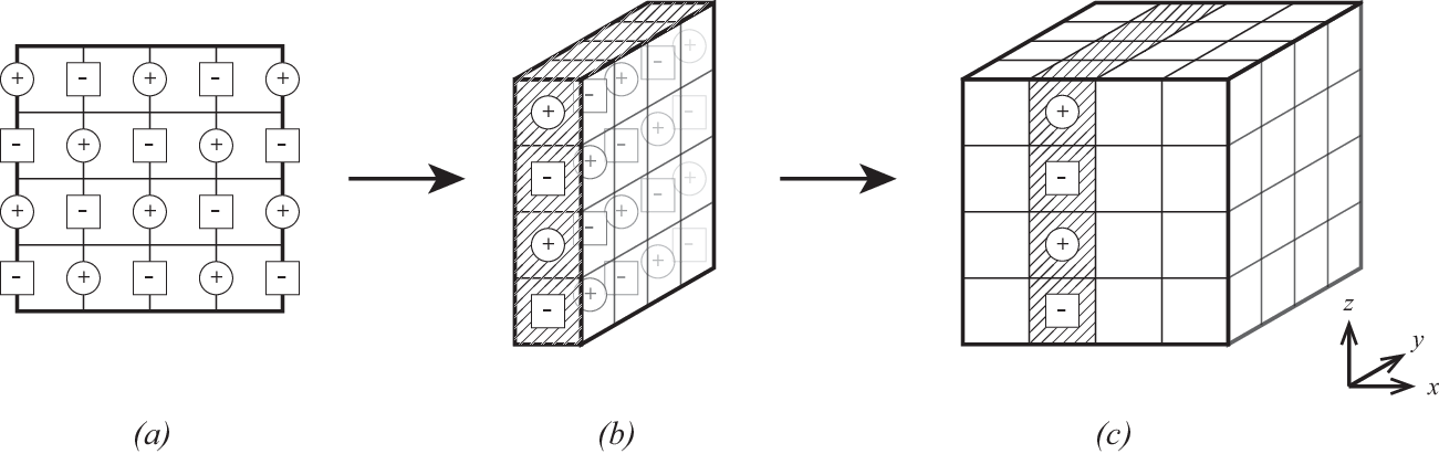
Due to the same reason discussed in the 2D case, an induced relation between boundary barycenter values on a strip perpendicular to the xx-axis can help to impose the periodic BC only when both NyN_{y} and NzN_{z} are even. In this case, coincidence of two barycenter values of the last boundary face pair is naturally achieved by pairwise coincidence of barycenter values of other boundary face pairs in the strip. Consequently, totally NxN_{x} periodic BCs can hold naturally due to other periodic BCs and induced boundary relations on strips perpendicular to the xx-axis. Similar claims hold for induced boundary relations on strips topologically perpendicular to yy-, and zz-directional axes.

However, as discussed in the case of Dirichlet BC, due to the linear dependence between Nx+Ny+NzN_{x}+N_{y}+N_{z} induced relations on all strips we have to consider 11 redundant relation when all Nx+Ny+NzN_{x}+N_{y}+N_{z} strips are taken into account of i.e., all NxN_{x}, NyN_{y} and NzN_{z} are even. This completes the proof.

6.2 Linear dependence of 𝔅\mathfrak{B} in 3D

In this section, we identify a global coefficient representation for node–based functions in 𝔅\mathfrak{B} with a vector in ℝ|𝔅|\mathbb{R}^{|\mathfrak{B}|}. With this identification, we use a vector 𝐜∈ℝ|𝔅|\mathbf{c}\in\mathbb{R}^{|\mathfrak{B}|} to represent a global coefficient representation on given 3D grid 𝒯h{\mathcal{T}}_{h}. In this sense, we denote the local coefficients of 𝐜\mathbf{c} in Q∈𝒯hQ\in{\mathcal{T}}_{h} by 𝐜|Q\left.\mathbf{c}\right|_{Q}. For the sake of simple description, we use this abusive notation as long as there is no chance of misunderstanding. A surjective linear map Bh𝔅:ℝ|𝔅|→V#𝔅,hB^{\mathfrak{B}}_{h}:\mathbb{R}^{|\mathfrak{B}|}\rightarrow V^{\mathfrak{B},h}_{\#} defined in Section 4 is obviously extended to the 3D case.

Figure 6.2: Nontrivial representations for the zero function in an element: 𝒜\mathcal{A}, 𝒳\mathcal{X}, 𝒴\mathcal{Y}, 𝒵\mathcal{Z}

As shown in Figure 6.2, there are exactly 4 kinds of local coefficient representation for the zero function in a single element. The value at each vertex represents the coefficient for the corresponding node–based function in 𝔅\mathfrak{B}. If any global coefficient representation for the zero function is restricted in an element, then it has to be a linear combination of these 4 elementary representations which are denoted by 𝒜,𝒳,𝒴\mathcal{A},\mathcal{X},\mathcal{Y} and 𝒵\mathcal{Z}, respectively. In other words, any global representation for the zero function is obtained by a consecutive extension of local representation in an appropriate way.

For D=𝒜,𝒳∪𝒜,𝒴∪𝒜,𝒵∪𝒜,𝒳∪𝒴∪𝒵∪𝒜,D=\mathcal{A},\mathcal{X}\cup\mathcal{A},\mathcal{Y}\cup\mathcal{A},\mathcal{Z}\cup\mathcal{A},\mathcal{X}\cup\mathcal{Y}\cup\mathcal{Z}\cup\mathcal{A}, designate 𝒮𝒟\mathcal{S}_{\mathcal{D}} the following subspace consisting of global representation:

𝒮𝒟:={𝐜∈ℝ|𝔅||𝐜|Q∈Span⁡{𝒟}​∀Q∈𝒯h}.\displaystyle\mathcal{S}_{\mathcal{D}}:=\left\{\mathbf{c}\in\mathbb{R}^{|\mathfrak{B}|}~|~\left.\mathbf{c}\right|_{Q}\in\operatorname{Span}\{\mathcal{D}\}\,\forall Q\in{\mathcal{T}}_{h}\right\}.
Remark 24.

The definition of Bh𝔅B^{\mathfrak{B}}_{h} implies ker⁡Bh𝔅=𝒮𝒳∪𝒴∪𝒵∪𝒜\ker B^{\mathfrak{B}}_{h}=\mathcal{S}_{\mathcal{X}\cup\mathcal{Y}\cup\mathcal{Z}\cup\mathcal{A}}.

We then have the following matching conditions on every face which is shared by two adjacent elements.

Lemma 25.

Let 𝐜∈𝒮𝒳∪𝒴∪𝒵∪𝒜\mathbf{c}\in\mathcal{S}_{\mathcal{X}\cup\mathcal{Y}\cup\mathcal{Z}\cup\mathcal{A}}, and ci​j​k𝒳,ci​j​k𝒴,ci​j​k𝒵,ci​j​k𝒜c^{\mathcal{X}}_{ijk},c^{\mathcal{Y}}_{ijk},c^{\mathcal{Z}}_{ijk},c^{\mathcal{A}}_{ijk} denote coefficients of 𝐜\mathbf{c} in an element Qi​j​k∈𝒯hQ_{ijk}\in{\mathcal{T}}_{h} for 𝒳\mathcal{X}, 𝒴\mathcal{Y}, 𝒵\mathcal{Z}, 𝒜\mathcal{A}, respectively, i.e., 𝐜|Qi​j​k=ci​j​k𝒳​𝒳+ci​j​k𝒴​𝒴+ci​j​k𝒵​𝒵+ci​j​k𝒜​𝒜.\left.\mathbf{c}\right|_{Q_{ijk}}=c^{\mathcal{X}}_{ijk}\mathcal{X}+c^{\mathcal{Y}}_{ijk}\mathcal{Y}+c^{\mathcal{Z}}_{ijk}\mathcal{Z}+c^{\mathcal{A}}_{ijk}\mathcal{A}. Then for all 1≤i≤Nx1\leq i\leq N_{x}, 1≤j≤Ny1\leq j\leq N_{y}, 1≤k≤Nz1\leq k\leq N_{z},

(6.2) ci​j​k𝒳−ci​j​k𝒜=c(i+1)​j​k𝒳+c(i+1)​j​k𝒜,ci​j​k𝒴=−c(i+1)​j​k𝒴,ci​j​k𝒵=−c(i+1)​j​k𝒵,ci​j​k𝒴−ci​j​k𝒜=ci⁡(j+1)​k𝒴+ci⁡(j+1)​k𝒜,ci​j​k𝒵=−ci⁡(j+1)​k𝒵,ci​j​k𝒳=−ci⁡(j+1)​k𝒳,ci​j​k𝒵−ci​j​k𝒜=ci​j​(k+1)𝒵+ci​j​(k+1)𝒜;ci​j​k𝒳=−ci​j​(k+1)𝒳;ci​j​k𝒴=−ci​j​(k+1)𝒴.&c^{\mathcal{X}}_{ijk}-c^{\mathcal{A}}_{ijk}=c^{\mathcal{X}}_{(i+1)jk}+c^{\mathcal{A}}_{(i+1)jk},\quad c^{\mathcal{Y}}_{ijk}=-c^{\mathcal{Y}}_{(i+1)jk},\quad c^{\mathcal{Z}}_{ijk}=-c^{\mathcal{Z}}_{(i+1)jk},\\ c^{\mathcal{Y}}_{ijk}-c^{\mathcal{A}}_{ijk}=c^{\mathcal{Y}}_{i(j+1)k}+c^{\mathcal{A}}_{i(j+1)k},\quad c^{\mathcal{Z}}_{ijk}=-c^{\mathcal{Z}}_{i(j+1)k},\quad c^{\mathcal{X}}_{ijk}=-c^{\mathcal{X}}_{i(j+1)k},\\ c^{\mathcal{Z}}_{ijk}-c^{\mathcal{A}}_{ijk}=c^{\mathcal{Z}}_{ij(k+1)}+c^{\mathcal{A}}_{ij(k+1)};\quad c^{\mathcal{X}}_{ijk}=-c^{\mathcal{X}}_{ij(k+1)};\quad c^{\mathcal{Y}}_{ijk}=-c^{\mathcal{Y}}_{ij(k+1)}.

Here all indices are understood up to modulo NxN_{x}, NyN_{y}, NzN_{z}, respectively, due to periodicity.

Remark 26.

Conversely, local relations (6.2)–(6.2) in Lemma 25 for all 1≤i≤Nx1\leq i\leq N_{x}, 1≤j≤Ny1\leq j\leq N_{y}, 1≤k≤Nz1\leq k\leq N_{z} imply the well-definedness of 𝐜∈𝒮𝒳∪𝒴∪𝒵∪𝒜\mathbf{c}\in\mathcal{S}_{\mathcal{X}\cup\mathcal{Y}\cup\mathcal{Z}\cup\mathcal{A}}, i.e., on each face shared by two adjacent elements the vertex values are matching.

Proof of Lemma 25.

Two elements Qi​j​kQ_{ijk} and Q(i+1)​j​kQ_{(i+1)jk} are adjacent in the topological xx-direction, and sharing a common face topologically perpendicular to the xx-axis. Thus the vertex values on the right face of the topologically left element Qi​j​kQ_{ijk} have to be matched with the vertex values on the the topologically left face of the topologically right element Q(i+1)​j​kQ_{(i+1)jk}. Since there are 4 nodes in the common face, we have 4 equations in 8 variables:

(6.3a) −ci​j​k𝒳+ci​j​k𝒴+ci​j​k𝒵+ci​j​k𝒜\displaystyle-c^{\mathcal{X}}_{ijk}+c^{\mathcal{Y}}_{ijk}+c^{\mathcal{Z}}_{ijk}+c^{\mathcal{A}}_{ijk} =−c(i+1)​j​k𝒳−c(i+1)​j​k𝒴−c(i+1)​j​k𝒵−c(i+1)​j​k𝒜,\displaystyle=-c^{\mathcal{X}}_{(i+1)jk}-c^{\mathcal{Y}}_{(i+1)jk}-c^{\mathcal{Z}}_{(i+1)jk}-c^{\mathcal{A}}_{(i+1)jk},
(6.3b) ci​j​k𝒳+ci​j​k𝒴−ci​j​k𝒵−ci​j​k𝒜\displaystyle c^{\mathcal{X}}_{ijk}+c^{\mathcal{Y}}_{ijk}-c^{\mathcal{Z}}_{ijk}-c^{\mathcal{A}}_{ijk} =c(i+1)​j​k𝒳−c(i+1)​j​k𝒴+c(i+1)​j​k𝒵+c(i+1)​j​k𝒜,\displaystyle=\phantom{+}c^{\mathcal{X}}_{(i+1)jk}-c^{\mathcal{Y}}_{(i+1)jk}+c^{\mathcal{Z}}_{(i+1)jk}+c^{\mathcal{A}}_{(i+1)jk},
(6.3c) ci​j​k𝒳−ci​j​k𝒴+ci​j​k𝒵−ci​j​k𝒜\displaystyle c^{\mathcal{X}}_{ijk}-c^{\mathcal{Y}}_{ijk}+c^{\mathcal{Z}}_{ijk}-c^{\mathcal{A}}_{ijk} =c(i+1)​j​k𝒳+c(i+1)​j​k𝒴−c(i+1)​j​k𝒵+c(i+1)​j​k𝒜,\displaystyle=\phantom{+}c^{\mathcal{X}}_{(i+1)jk}+c^{\mathcal{Y}}_{(i+1)jk}-c^{\mathcal{Z}}_{(i+1)jk}+c^{\mathcal{A}}_{(i+1)jk},
(6.3d) −ci​j​k𝒳−ci​j​k𝒴−ci​j​k𝒵+ci​j​k𝒜\displaystyle-c^{\mathcal{X}}_{ijk}-c^{\mathcal{Y}}_{ijk}-c^{\mathcal{Z}}_{ijk}+c^{\mathcal{A}}_{ijk} =−c(i+1)​j​k𝒳+c(i+1)​j​k𝒴+c(i+1)​j​k𝒵−c(i+1)​j​k𝒜.\displaystyle=-c^{\mathcal{X}}_{(i+1)jk}+c^{\mathcal{Y}}_{(i+1)jk}+c^{\mathcal{Z}}_{(i+1)jk}-c^{\mathcal{A}}_{(i+1)jk}.

Simple calculation shows that (6.3) are equivalent to (6.2). Similarly, considering faces topologically perpendicular to the yy- and zz-directions, we get (6.2) and (6.2), respectively.

The next decomposition theorem is essential for the dimension analysis in the 3D case.

Theorem 27 (Decomposition Theorem).

The quotient space 𝒮𝒳∪𝒴∪𝒵∪𝒜/𝒮𝒜\mathcal{S}_{\mathcal{X}\cup\mathcal{Y}\cup\mathcal{Z}\cup\mathcal{A}}/\mathcal{S}_{\mathcal{A}} can be decomposed as

(6.4) 𝒮𝒳∪𝒴∪𝒵∪𝒜/𝒮𝒜=𝒮𝒳∪𝒜/𝒮𝒜⊕𝒮𝒴∪𝒜/𝒮𝒜⊕𝒮𝒵∪𝒜/𝒮𝒜.\displaystyle\mathcal{S}_{\mathcal{X}\cup\mathcal{Y}\cup\mathcal{Z}\cup\mathcal{A}}/\mathcal{S}_{\mathcal{A}}=\mathcal{S}_{\mathcal{X}\cup\mathcal{A}}/\mathcal{S}_{\mathcal{A}}\oplus\mathcal{S}_{\mathcal{Y}\cup\mathcal{A}}/\mathcal{S}_{\mathcal{A}}\oplus\mathcal{S}_{\mathcal{Z}\cup\mathcal{A}}/\mathcal{S}_{\mathcal{A}}.

Proof.

It is clear that 𝒮𝒜⊂𝒮𝒳∪𝒜,𝒮𝒴∪𝒜,𝒮𝒵∪𝒜⊂𝒮𝒳∪𝒴∪𝒵∪𝒜\mathcal{S}_{\mathcal{A}}\subset\mathcal{S}_{\mathcal{X}\cup\mathcal{A}},\mathcal{S}_{\mathcal{Y}\cup\mathcal{A}},\mathcal{S}_{\mathcal{Z}\cup\mathcal{A}}\subset\mathcal{S}_{\mathcal{X}\cup\mathcal{Y}\cup\mathcal{Z}\cup\mathcal{A}} and 𝒮𝒳∪𝒜∩𝒮𝒴∪𝒜=𝒮𝒴∪𝒜∩𝒮𝒵∪𝒜=𝒮𝒵∪𝒜∩𝒮𝒳∪𝒜=𝒮𝒜\mathcal{S}_{\mathcal{X}\cup\mathcal{A}}\cap\mathcal{S}_{\mathcal{Y}\cup\mathcal{A}}=\mathcal{S}_{\mathcal{Y}\cup\mathcal{A}}\cap\mathcal{S}_{\mathcal{Z}\cup\mathcal{A}}=\mathcal{S}_{\mathcal{Z}\cup\mathcal{A}}\cap\mathcal{S}_{\mathcal{X}\cup\mathcal{A}}=\mathcal{S}_{\mathcal{A}}. Thus it is enough to show that for any 𝐜∈𝒮𝒳∪𝒴∪𝒵∪𝒜\mathbf{c}\in\mathcal{S}_{\mathcal{X}\cup\mathcal{Y}\cup\mathcal{Z}\cup\mathcal{A}}, there exist 𝐮∈𝒮𝒳∪𝒜\mathbf{u}\in\mathcal{S}_{\mathcal{X}\cup\mathcal{A}}, 𝐯∈𝒮𝒴∪𝒜\mathbf{v}\in\mathcal{S}_{\mathcal{Y}\cup\mathcal{A}}, 𝐰∈𝒮𝒵∪𝒜\mathbf{w}\in\mathcal{S}_{\mathcal{Z}\cup\mathcal{A}} such that 𝐜∈𝐮+𝐯+𝐰+𝒮𝒜.\mathbf{c}\in\mathbf{u}+\mathbf{v}+\mathbf{w}+\mathcal{S}_{\mathcal{A}}.

Let ci​j​k𝒳c^{\mathcal{X}}_{ijk}, ci​j​k𝒴c^{\mathcal{Y}}_{ijk}, ci​j​k𝒵c^{\mathcal{Z}}_{ijk}, ci​j​k𝒜c^{\mathcal{A}}_{ijk} denote the coefficients of 𝐜\mathbf{c} in Qi​j​k∈𝒯hQ_{ijk}\in{\mathcal{T}}_{h} for 𝒳\mathcal{X}, 𝒴\mathcal{Y}, 𝒵\mathcal{Z}, 𝒜\mathcal{A}, respectively, i.e., 𝐜|Qi​j​k=ci​j​k𝒳​𝒳+ci​j​k𝓃​𝒴​𝒴+ci​j​k𝒵​𝒵+ci​j​k𝒜​𝒜.\left.\mathbf{c}\right|_{Q_{ijk}}=c^{\mathcal{X}}_{ijk}\mathcal{X}+c^{\mathcal{nY}}_{ijk}\mathcal{Y}+c^{\mathcal{Z}}_{ijk}\mathcal{Z}+c^{\mathcal{A}}_{ijk}\mathcal{A}. Due to Lemma 25, the relations (6.2)–(6.2) hold. Now we construct 𝐮\mathbf{u}, 𝐯\mathbf{v}, and 𝐰\mathbf{w}. First, define 𝐮∈ℝ|𝔅|\mathbf{u}\in\mathbb{R}^{|\mathfrak{B}|} by

(6.5) 𝐮|Qi​j​k:=ui​j​k𝒳​𝒳+ui​j​k𝒜​𝒜whereui​j​k𝒳=ci​j​k𝒳,ui​j​k𝒜=(−1)j+k​ci​11𝒜.\displaystyle\left.\mathbf{u}\right|_{Q_{ijk}}:=u^{\mathcal{X}}_{ijk}\mathcal{X}+u^{\mathcal{A}}_{ijk}\mathcal{A}\quad\text{where}\quad u^{\mathcal{X}}_{ijk}=c^{\mathcal{X}}_{ijk},u^{\mathcal{A}}_{ijk}=(-1)^{j+k}c^{\mathcal{A}}_{i11}.

We have ui​j​k𝒴=ui​j​k𝒵=0u^{\mathcal{Y}}_{ijk}=u^{\mathcal{Z}}_{ijk}=0. We can check the followings.

  1. 1.

    𝐮\mathbf{u} is well-defined, and belongs to 𝒮𝒳∪𝒴∪𝒵∪𝒜\mathcal{S}_{\mathcal{X}\cup\mathcal{Y}\cup\mathcal{Z}\cup\mathcal{A}}: See Remark 26. For a face shared by two adjacent elements Qi​j​kQ_{ijk} and Q(i+1)​j​kQ_{(i+1)jk},

    ui​j​k𝒳−ui​j​k𝒜\displaystyle u^{\mathcal{X}}_{ijk}-u^{\mathcal{A}}_{ijk} =ci​j​k𝒳−(−1)j+k​ci​11𝒜\displaystyle=c^{\mathcal{X}}_{ijk}-(-1)^{j+k}c^{\mathcal{A}}_{i11}
    =c(i+1)​j​k𝒳+(−1)j+k​c(i+1)​11𝒜=u(i+1)​j​k𝒳+u(i+1)​j​k𝒜.\displaystyle=c^{\mathcal{X}}_{(i+1)jk}+(-1)^{j+k}c^{\mathcal{A}}_{(i+1)11}=u^{\mathcal{X}}_{(i+1)jk}+u^{\mathcal{A}}_{(i+1)jk}.

    Thus 𝐮\mathbf{u} is matching on all faces perpendicular to the xx-axis. For the faces perpendicular to the yy-axis, we have

    ui​j​k𝒳=ci​j​k𝒳=−ci⁡(j+1)​k𝒳=−ui⁡(j+1)​k𝒳,\displaystyle u^{\mathcal{X}}_{ijk}=c^{\mathcal{X}}_{ijk}=-c^{\mathcal{X}}_{i(j+1)k}=-u^{\mathcal{X}}_{i(j+1)k},
    −ui​j​k𝒜=−(−1)j+k​ci​11𝒜=(−1)j+1+k​ci​11𝒜=ui⁡(j+1)​k𝒜,\displaystyle-u^{\mathcal{A}}_{ijk}=-(-1)^{j+k}c^{\mathcal{A}}_{i11}=(-1)^{j+1+k}c^{\mathcal{A}}_{i11}=u^{\mathcal{A}}_{i(j+1)k},

    and similar for the faces perpendicular to the zz-axis. Therefore 𝐮\mathbf{u} is also matching along the yy- and zz-directions.

  2. 2.

    𝐮∈𝒮𝒳∪𝒜\mathbf{u}\in\mathcal{S}_{\mathcal{X}\cup\mathcal{A}}: It is trivial due to the definition of 𝐮\mathbf{u} and 𝒮𝒳∪𝒜\mathcal{S}_{\mathcal{X}\cup\mathcal{A}}.

Similarly to 𝐮\mathbf{u}, we define 𝐯\mathbf{v} and 𝐰∈ℝ|𝔅|\mathbf{w}\in\mathbb{R}^{|\mathfrak{B}|} by

𝐯|Qi​j​k:=vi​j​k𝒴​𝒴+vi​j​k𝒜​𝒜wherevi​j​k𝒴=ci​j​k𝒴,vi​j​k𝒜=(−1)i+k​c1​j​1𝒜,\displaystyle\left.\mathbf{v}\right|_{Q_{ijk}}:=v^{\mathcal{Y}}_{ijk}\mathcal{Y}+v^{\mathcal{A}}_{ijk}\mathcal{A}\quad\text{where}\quad v^{\mathcal{Y}}_{ijk}=c^{\mathcal{Y}}_{ijk},v^{\mathcal{A}}_{ijk}=(-1)^{i+k}c^{\mathcal{A}}_{1j1},
𝐰|Qi​j​k:=wi​j​k𝒵​𝒵+wi​j​k𝒜​𝒜wherewi​j​k𝒵=ci​j​k𝒵,wi​j​k𝒜=(−1)i+j​c11​k𝒜.\displaystyle\left.\mathbf{w}\right|_{Q_{ijk}}:=w^{\mathcal{Z}}_{ijk}\mathcal{Z}+w^{\mathcal{A}}_{ijk}\mathcal{A}\quad\text{where}\quad w^{\mathcal{Z}}_{ijk}=c^{\mathcal{Z}}_{ijk},w^{\mathcal{A}}_{ijk}=(-1)^{i+j}c^{\mathcal{A}}_{11k}.

Then both 𝐯\mathbf{v} and 𝐰\mathbf{w} are well-defined, and 𝐯∈𝒮𝒴∪𝒜\mathbf{v}\in\mathcal{S}_{\mathcal{Y}\cup\mathcal{A}}, 𝐰∈𝒮𝒵∪𝒜\mathbf{w}\in\mathcal{S}_{\mathcal{Z}\cup\mathcal{A}}. Thus 𝐜−(𝐮+𝐯+𝐰)∈𝒮𝒳∪𝒴∪𝒵∪𝒜\mathbf{c}-(\mathbf{u}+\mathbf{v}+\mathbf{w})\in\mathcal{S}_{\mathcal{X}\cup\mathcal{Y}\cup\mathcal{Z}\cup\mathcal{A}}. We can conclude 𝐜−(𝐮+𝐯+𝐰)∈𝒮𝒜\mathbf{c}-(\mathbf{u}+\mathbf{v}+\mathbf{w})\in\mathcal{S}_{\mathcal{A}} since for each Qi​j​kQ_{ijk},

𝐜−(𝐮+𝐯+𝐰)|Qi​j​k=(ci​j​k𝒜−(−1)j+k​ci​11𝒜−(−1)i+k​c1​j​1𝒜−(−1)i+j​c11​k𝒜)​𝒜.\displaystyle\left.\mathbf{c}-(\mathbf{u}+\mathbf{v}+\mathbf{w})\right|_{Q_{ijk}}=\left(c^{\mathcal{A}}_{ijk}-(-1)^{j+k}c^{\mathcal{A}}_{i11}-(-1)^{i+k}c^{\mathcal{A}}_{1j1}-(-1)^{i+j}c^{\mathcal{A}}_{11k}\right)\mathcal{A}.

Corollary 28.

dim⁡ker⁡Bh𝔅=dim⁡𝒮𝒳∪𝒜+dim⁡𝒮𝒴∪𝒜+dim⁡𝒮𝒵∪𝒜−2​dim​𝒮𝒜\operatorname{dim}\,\ker B^{\mathfrak{B}}_{h}=\operatorname{dim}\,\mathcal{S}_{\mathcal{X}\cup\mathcal{A}}+\operatorname{dim}\,\mathcal{S}_{\mathcal{Y}\cup\mathcal{A}}+\operatorname{dim}\,\mathcal{S}_{\mathcal{Z}\cup\mathcal{A}}-2\operatorname{dim}\,\mathcal{S}_{\mathcal{A}}.

The following lemmas explain the dimension of subspaces which depends on parity of the discretization numbers.

Lemma 29.

(The dimension of 𝒮𝒳∪𝒜\mathcal{S}_{\mathcal{X}\cup\mathcal{A}}, 𝒮𝒴∪𝒜\mathcal{S}_{\mathcal{Y}\cup\mathcal{A}}, 𝒮𝒵∪𝒜\mathcal{S}_{\mathcal{Z}\cup\mathcal{A}})

(6.6) dim⁡𝒮𝒳∪𝒜=Nx​𝔢​(Ny)​𝔢​(Nz),dim⁡𝒮𝒴∪𝒜=𝔢⁡(Nx)​Ny​𝔢​(Nz),dim⁡𝒮𝒵∪𝒜=𝔢⁡(Nx)​𝔢​(Ny)​Nz.\operatorname{dim}\,\mathcal{S}_{\mathcal{X}\cup\mathcal{A}}&=N_{x}\mathfrak{e}(N_{y})\mathfrak{e}(N_{z}),\\ \operatorname{dim}\,\mathcal{S}_{\mathcal{Y}\cup\mathcal{A}}=\mathfrak{e}(N_{x})N_{y}\mathfrak{e}(N_{z}),\\ \operatorname{dim}\,\mathcal{S}_{\mathcal{Z}\cup\mathcal{A}}=\mathfrak{e}(N_{x})\mathfrak{e}(N_{y})N_{z}.

Proof.

It is enough to show the claim for 𝒮𝒳∪𝒜\mathcal{S}_{\mathcal{X}\cup\mathcal{A}}, since the others are similar. Let 𝐜∈𝒮𝒳∪𝒜\mathbf{c}\in\mathcal{S}_{\mathcal{X}\cup\mathcal{A}} where 𝐜|Qi​j​k=ci​j​k𝒳​𝒳+ci​j​k𝒜​𝒜\left.\mathbf{c}\right|_{Q_{ijk}}=c^{\mathcal{X}}_{ijk}\mathcal{X}+c^{\mathcal{A}}_{ijk}\mathcal{A} in each cube Qi​j​k∈𝒯hQ_{ijk}\in{\mathcal{T}}_{h}. By applying the matching conditions (6.2) and (6.2) consecutively, it can be shown

ci​j​k𝒳=(−1)j+k​ci​11𝒳andci​j​k𝒜=(−1)j+k​ci​11𝒜.\displaystyle c^{\mathcal{X}}_{ijk}=(-1)^{j+k}c^{\mathcal{X}}_{i11}\quad\text{and}\quad c^{\mathcal{A}}_{ijk}=(-1)^{j+k}c^{\mathcal{A}}_{i11}.

Consider Nx+1N_{x}+1 combined surfaces such that each of them consists of Ny×NzN_{y}\times N_{z} faces in 𝒯h{\mathcal{T}}_{h}, and is lying on the same hyperplane perpendicular to the xx-axis. The above relations imply that on each surface the coefficients for node–based functions are all the same, but with alternating sign like a checkerboard pattern at nodes, not on faces. Due to the identification between boundary nodes in the yy- and zz-directions, all coefficients vanish unless both NyN_{y} and NzN_{z} are even.

Under the case of even NyN_{y} and NzN_{z}, we consider a basis checkerboard pattern at nodes on a combined surface consisting of +1+1 and −1-1, alternatively, as Figure 6.3 (a) shows. In the figure, the plus and minus sign at nodes represent the positive value one, and the negative value one, respectively. We get Nx+1N_{x}+1 checkerboard patterns on Nx+1N_{x}+1 combined surfaces in series (Figure 6.3 (b)). Based on the basis checkerboard pattern described above, we can represent all coefficients on each combined surface by a single factor in real number. Due to the identification between boundary nodes in the xx-direction, factors for the first and the last combined surface must be same. Then the series of Nx+1N_{x}+1 checkerboard patterns compose a global representation for a function in 𝒮𝒳∪𝒜\mathcal{S}_{\mathcal{X}\cup\mathcal{A}} (Figure 6.3 (c)). Conversely, for the Nx+1N_{x}+1 combined surfaces which are perpendicular to the xx-axis and the basis checkerboard pattern at nodes on surfaces, suppose Nx+1N_{x}+1 factors are given, where the first and the last of them are same. Then we can determine unique ci​j​k𝒳c^{\mathcal{X}}_{ijk} and ci​j​k𝒜c^{\mathcal{A}}_{ijk}, for all Qi​j​k∈𝒯hQ_{ijk}\in{\mathcal{T}}_{h}. Therefore, only in the case when both NyN_{y} and NzN_{z} are even, 𝒮𝒳∪𝒜\mathcal{S}_{\mathcal{X}\cup\mathcal{A}} is equivalent to {𝐯∈ℝNx+1|v1=vNx+1}\{\mathbf{v}\in\mathbb{R}^{N_{x}+1}~|~v_{1}=v_{N_{x}+1}\} and dim⁡𝒮𝒳∪𝒜=Nx\operatorname{dim}\,\mathcal{S}_{\mathcal{X}\cup\mathcal{A}}=N_{x} consequently.

Refer to caption
Figure 6.3: Construction of a global representation for a function in 𝒮𝒳∪𝒜\mathcal{S}_{\mathcal{X}\cup\mathcal{A}}
Lemma 30.

(The dimension of 𝒮𝒜\mathcal{S}_{\mathcal{A}})

(6.7) dim⁡𝒮𝒜=𝔢⁡(Nx)​𝔢​(Ny)​𝔢​(Nz).\displaystyle\operatorname{dim}\,\mathcal{S}_{\mathcal{A}}=\mathfrak{e}(N_{x})\mathfrak{e}(N_{y})\mathfrak{e}(N_{z}).

Proof.

Let 𝐜∈𝒮𝒜\mathbf{c}\in\mathcal{S}_{\mathcal{A}} where 𝐜|Qi​j​k=ci​j​k𝒜​𝒜\left.\mathbf{c}\right|_{Q_{ijk}}=c^{\mathcal{A}}_{ijk}\mathcal{A} in each cube Qi​j​kQ_{ijk}. By applying the matching conditions (6.2)–(6.2) consecutively, it is shown ci​j​k𝒜=(−1)i+j+k+1​c111𝒜.c^{\mathcal{A}}_{ijk}=(-1)^{i+j+k+1}c^{\mathcal{A}}_{111}. Due to the identification of boundary nodes in the xx-, yy-, and zz-directions, all coefficients vanish unless all NxN_{x}, NyN_{y} and NzN_{z} are even. In the case of all even NxN_{x}, NyN_{y} and NzN_{z}, it is easily shown that the coefficients form a multiple of the 3D checkerboard pattern at nodes. Therefore dim⁡𝒮𝒜=1\operatorname{dim}\,\mathcal{S}_{\mathcal{A}}=1.

The following proposition is a direct consequence of , Lemmas 29 and  30.

Proposition 31.

(The dimensions of ker⁡Bh𝔅\ker B^{\mathfrak{B}}_{h}, V#𝔅,hV^{\mathfrak{B},h}_{\#} in 3D)

dim⁡ker⁡Bh𝔅\displaystyle\operatorname{dim}\,\ker B^{\mathfrak{B}}_{h} =\displaystyle= Nx​𝔢​(Ny)​𝔢​(Nz)+𝔢⁡(Nx)​Ny​𝔢​(Nz)+𝔢⁡(Nx)​𝔢​(Ny)​Nz−2​𝔢​(Nx)​𝔢​(Ny)​𝔢​(Nz),\displaystyle N_{x}\mathfrak{e}(N_{y})\mathfrak{e}(N_{z})+\mathfrak{e}(N_{x})N_{y}\mathfrak{e}(N_{z})+\mathfrak{e}(N_{x})\mathfrak{e}(N_{y})N_{z}-2\mathfrak{e}(N_{x})\mathfrak{e}(N_{y})\mathfrak{e}(N_{z}),
dim⁡V#𝔅,h\displaystyle\operatorname{dim}\,V^{\mathfrak{B},h}_{\#} =\displaystyle= NxNyNz−[Nx𝔢(Ny)𝔢(Nz)+𝔢(Nx)Ny𝔢(Nz)+𝔢(Nx)𝔢(Ny)Nz\displaystyle N_{x}N_{y}N_{z}-\left[N_{x}\mathfrak{e}(N_{y})\mathfrak{e}(N_{z})+\mathfrak{e}(N_{x})N_{y}\mathfrak{e}(N_{z})+\mathfrak{e}(N_{x})\mathfrak{e}(N_{y})N_{z}\right.
−2𝔢(Nx)𝔢(Ny)𝔢(Nz)].\displaystyle\left.\qquad\qquad-2\mathfrak{e}(N_{x})\mathfrak{e}(N_{y})\mathfrak{e}(N_{z})\right].

6.3 A basis for V#hV^{h}_{\#} in 3D

Propositions 23 and  31 imply that V#𝔅,hV^{\mathfrak{B},h}_{\#} is a proper subset of V#hV^{h}_{\#} if at most one of NxN_{x}, NyN_{y}, and NzN_{z} is odd. Furthermore, if all NxN_{x}, NyN_{y}, and NzN_{z} are even, then there exist 2​(Nx+Ny+Nz)−32(N_{x}+N_{y}+N_{z})-3 complementary basis functions for V#hV^{h}_{\#}, not belonging to V#𝔅,hV^{\mathfrak{B},h}_{\#}. If only NιN_{\iota} is odd, then the number of complementary basis functions for V#hV^{h}_{\#} is 2​Nι2N_{\iota}. In other cases, V#𝔅,hV^{\mathfrak{B},h}_{\#} is equal to V#hV^{h}_{\#}. We will discuss about the complementary basis functions below.

Theorem 32.

(A complementary basis for V#hV^{h}_{\#} in 3D) Suppose a rectangular domain Ω\Omega is given with a triangulation 𝒯h{\mathcal{T}}_{h}, consisting of cubes, in which the number of elements along coordinates are NxN_{x}, NyN_{y}, NzN_{z}. For given 1≤i≤Nx1\leq i\leq N_{x}, let Ωix\Omega^{x}_{i} be the subdomain consisting of Ny×NzN_{y}\times N_{z} cubes whose discrete position in xx–coordinate are all same to ii. Let (ψix)y(\psi^{x}_{i})_{y} denote a piecewise linear function in V#hV^{h}_{\#}, whose support is Ωix\Omega^{x}_{i}, such that it has nonzero barycenter values only on faces perpendicular to the yy-axis, and all the nonzero barycenter values are 11 with alternating sign in the yy- and zz-directions. We can consider (ψix)z(\psi^{x}_{i})_{z}, (ψjy)x(\psi^{y}_{j})_{x}, (ψjy)z(\psi^{y}_{j})_{z}, (ψkz)x(\psi^{z}_{k})_{x}, (ψkz)y(\psi^{z}_{k})_{y} in similar manner. The followings hold.

  1. 1.

    If all NxN_{x}, NyN_{y}, and NzN_{z} are even, then V#𝔅,hV^{\mathfrak{B},h}_{\#} is a proper subset of V#hV^{h}_{\#}. The union of

    • •

      any Nx+Ny−1N_{x}+N_{y}-1 among 𝔄z:={(ψix)z,(ψjy)z}1≤i≤Nx,1≤j≤Ny\mathfrak{A}_{z}:=\{(\psi^{x}_{i})_{z},(\psi^{y}_{j})_{z}\}_{1\leq i\leq N_{x},1\leq j\leq N_{y}},

    • •

      any Ny+Nz−1N_{y}+N_{z}-1 among 𝔄x:={(ψjy)x,(ψkz)x}1≤j≤Ny,1≤k≤Nz\mathfrak{A}_{x}:=\{(\psi^{y}_{j})_{x},(\psi^{z}_{k})_{x}\}_{1\leq j\leq N_{y},1\leq k\leq N_{z}}, and

    • •

      any Nz+Nx−1N_{z}+N_{x}-1 among 𝔄y:={(ψkz)y,(ψix)y}1≤i≤Nx,1≤k≤Nz\mathfrak{A}_{y}:=\{(\psi^{z}_{k})_{y},(\psi^{x}_{i})_{y}\}_{1\leq i\leq N_{x},1\leq k\leq N_{z}}

    is a complementary basis for V#hV^{h}_{\#}, not belonging to V#𝔅,hV^{\mathfrak{B},h}_{\#}.

  2. 2.

    If only NιN_{\iota} is odd (and Nμ,NνN_{\mu},N_{\nu} are even), then V#𝔅,hV^{\mathfrak{B},h}_{\#} is a proper subset of V#hV^{h}_{\#}. Moreover, {(ψjι)μ,(ψjι)ν}1≤j≤Nι\{(\psi^{\iota}_{j})_{\mu},(\psi^{\iota}_{j})_{\nu}\}_{1\leq j\leq N_{\iota}} is a complementary basis for V#hV^{h}_{\#}, which is not contained in V#𝔅,hV^{\mathfrak{B},h}_{\#}.

  3. 3.

    Otherwise, V#𝔅,h=V#hV^{\mathfrak{B},h}_{\#}=V^{h}_{\#}.

Proof.

For the first case, suppose that all NxN_{x}, NyN_{y}, and NzN_{z} are even. Note that all nonzero barycenter values of (ψix)y(\psi^{x}_{i})_{y} are lying on the faces perpendicular to only one axis with alternating sign, as similar to the alternating function ψx\psi_{x} in the 2D case (Figure 6.4 (a), (b)), and its support is Ωix\Omega^{x}_{i} (Figure 6.4 (c)). Using a similar argument as in the 2D case, it is easily shown that (ψix)y(\psi^{x}_{i})_{y} is well-defined, and not belonging to V#𝔅,hV^{\mathfrak{B},h}_{\#} since NyN_{y} and NzN_{z} are even. A similar property holds for (ψix)z(\psi^{x}_{i})_{z}, a piecewise linear function in V#hV^{h}_{\#} whose support is Ωix\Omega^{x}_{i} and which has nonzero barycenter values as 11 only on faces perpendicular to the zz-axis with alternating sign in the yy- and zz-directions. Thus there exist 2​Nx2N_{x} alternating functions, {(ψix)y,(ψix)z}1≤i≤Nx\{(\psi^{x}_{i})_{y},(\psi^{x}_{i})_{z}\}_{1\leq i\leq N_{x}}, for V#hV^{h}_{\#} associated with strips perpendicular to the xx-axis. By considering other strips perpendicular to the yy- or zz-axis, we can find out 2​(Nx+Ny+Nz)2(N_{x}+N_{y}+N_{z}) alternating functions for V#hV^{h}_{\#}, not belonging to V#𝔅,hV^{\mathfrak{B},h}_{\#}: {(ψix)y,(ψix)z,(ψjy)x,(ψjy)z,(ψkz)x,(ψkz)y}1≤i≤Nx,1≤j≤Ny,1≤k≤Nz\{(\psi^{x}_{i})_{y},(\psi^{x}_{i})_{z},(\psi^{y}_{j})_{x},(\psi^{y}_{j})_{z},(\psi^{z}_{k})_{x},(\psi^{z}_{k})_{y}\}_{1\leq i\leq N_{x},1\leq j\leq N_{y},1\leq k\leq N_{z}}.

However, there is a single relation between the alternating functions in each direction on subscript. An alternating sum of (ψix)z(\psi^{x}_{i})_{z} in 1≤i≤Nx1\leq i\leq N_{x} is equal to that of (ψjy)z(\psi^{y}_{j})_{z} in 1≤j≤Ny1\leq j\leq N_{y}. And any Nx+Ny−1N_{x}+N_{y}-1 among all (ψix)z(\psi^{x}_{i})_{z} and (ψjy)z(\psi^{y}_{j})_{z} are linearly independent due to their supports. Similarly, any Ny+Nz−1N_{y}+N_{z}-1 among all (ψjy)x(\psi^{y}_{j})_{x} and (ψkz)x(\psi^{z}_{k})_{x} are linearly independent, and so any Nz+Nx−1N_{z}+N_{x}-1 among all (ψkz)y(\psi^{z}_{k})_{y} and (ψix)y(\psi^{x}_{i})_{y} are. Consequently, suitably chosen 2​(Nx+Ny+Nz)−32(N_{x}+N_{y}+N_{z})-3 alternating functions form a complementary basis for V#hV^{h}_{\#}.

In the case of only one odd NιN_{\iota} (and even NμN_{\mu}, NνN_{\nu}), the set of all alternating functions associated to the strips perpendicular to the ι\iota-axis, {(ψjι)μ,(ψjι)ν}1≤j≤Nι\{(\psi^{\iota}_{j})_{\mu},(\psi^{\iota}_{j})_{\nu}\}_{1\leq j\leq N_{\iota}}, are meaningful because NμN_{\mu} and NνN_{\nu} are even.

Refer to caption
Figure 6.4: Construction of an alternating function in 3D

6.4 Stiffness matrix associated with 𝔅\mathfrak{B} in 3D

The stiffness matrix 𝐒h𝔅\mathbf{S}^{\mathfrak{B}}_{h} associated with 𝔅\mathfrak{B} is defined as in (4.5) but in 3D space. See Figure 6.5 for the 3D local stencil for the stiffness matrix associated with 𝔅\mathfrak{B}. Propositions 12 and  31 lead the following proposition.

Refer to caption
Figure 6.5: The stencil for 𝐒h𝔅\mathbf{S}^{\mathfrak{B}}_{h} with uniform cubes of size h×h×hh\times h\times h in 3D.
Proposition 33.

(The dimension of ker⁡𝐒h𝔅\ker\mathbf{S}^{\mathfrak{B}}_{h} in 3D)

dim⁡ker⁡𝐒h𝔅\displaystyle\operatorname{dim}\,\ker\mathbf{S}^{\mathfrak{B}}_{h} =Nx​𝔢​(Ny)​𝔢​(Nz)+𝔢⁡(Nx)​Ny​𝔢​(Nz)+𝔢⁡(Nx)​𝔢​(Ny)​Nz\displaystyle=N_{x}\mathfrak{e}(N_{y})\mathfrak{e}(N_{z})+\mathfrak{e}(N_{x})N_{y}\mathfrak{e}(N_{z})+\mathfrak{e}(N_{x})\mathfrak{e}(N_{y})N_{z}
−2​𝔢​(Nx)​𝔢​(Ny)​𝔢​(Nz)+1.\displaystyle\qquad\qquad-2\mathfrak{e}(N_{x})\mathfrak{e}(N_{y})\mathfrak{e}(N_{z})+1.

Let us assemble 𝐒h𝔅\mathbf{S}^{\mathfrak{B}}_{h} for various combinations of NxN_{x}, NyN_{y}, and NzN_{z}. The rank deficiency is computed by using MATLAB. Table 6.1 shows numerically obtained rank deficiency of 𝐒h𝔅\mathbf{S}^{\mathfrak{B}}_{h} in 3D space. Without loss of generality, it only represents combinations which hold Nx≥Ny≥NzN_{x}\geq N_{y}\geq N_{z}. Numbers in red, blue, and black represent the case of all even discretizations and the case of odd discretization in only one direction, and the other cases, respectively. These results imply that the rank deficiency pattern depend on parity combination and confirm our theoretical result in Proposition 33.

Nz=𝟐N_{z}={\bf 2} NyN_{y}
2 3 4 5 6 7 8
NxN_{x} 2 5
3 4 1
4 7 4 9
5 6 1 6 1
6 9 4 11 6 13
7 8 1 8 1 8 1
8 11 4 13 6 15 8 17
Nz=𝟒N_{z}={\bf 4}
2 3 4 5 6 7 8
2
3
4 11
5 6 1
6 13 6 15
7 8 1 8 1
8 15 6 17 8 19
Nz=3N_{z}=3
2 3 4 5 6 7 8
2
3 1
4 1 4
5 1 1 1
6 1 4 1 4
7 1 1 1 1 1
8 1 4 1 4 1 4
Nz=5N_{z}=5
2 3 4 5 6 7 8
2
3
4
5 1
6 1 6
7 1 1 1
8 1 6 1 6
Table 6.1: Numerically obtained rank deficiency of 𝐒h𝔅\mathbf{S}^{\mathfrak{B}}_{h} in 3D

6.5 Numerical schemes in 3D

Consider again an elliptic problem with periodic BC (5.1) with the compatibility condition ∫Ωf=0\int_{\Omega}f=0, the corresponding weak formulation (5.1), and the corresponding discrete weak formulation (5.2) in 3D.

Throughout this section, we assume that all NxN_{x}, NyN_{y}, and NzN_{z} are even.

Additional Notations & Properties

𝔅♭\mathfrak{B}^{\flat} again denotes a basis for V#𝔅,hV^{\mathfrak{B},h}_{\#}, a proper subset of 𝔅\mathfrak{B}. A constructive method for 𝔅♭\mathfrak{B}^{\flat} will be given. Let 𝔄\mathfrak{A} and 𝔄♭\mathfrak{A}^{\flat} be the set of all alternating functions, and a complementary basis for V#hV^{h}_{\#} which consists of alternating functions as in Theorem 32, respectively. Without loss of generality, we may write 𝔅♭={ϕj}j=1|𝔅♭|\mathfrak{B}^{\flat}=\{\phi_{j}\}_{j=1}^{|\mathfrak{B}^{\flat}|}, 𝔅={ϕj}j=1|𝔅|\mathfrak{B}=\{\phi_{j}\}_{j=1}^{|\mathfrak{B}|}, 𝔄♭={ψj}j=1|𝔄♭|\mathfrak{A}^{\flat}=\{\psi_{j}\}_{j=1}^{|\mathfrak{A}^{\flat}|}, and 𝔄={ψj}j=1|𝔄|\mathfrak{A}=\{\psi_{j}\}_{j=1}^{|\mathfrak{A}|}. Define two extended sets 𝔈:=𝔅∪𝔄\mathfrak{E}:=\mathfrak{B}\cup\mathfrak{A}, and 𝔈♭:=𝔅♭∪𝔄♭\mathfrak{E}^{\flat}:=\mathfrak{B}^{\flat}\cup\mathfrak{A}^{\flat}. Even in the 3D case, 𝔈♭\mathfrak{E}^{\flat} forms a basis for V#hV^{h}_{\#}. The characteristics of 𝔅♭\mathfrak{B}^{\flat}, 𝔅\mathfrak{B}, 𝔈♭\mathfrak{E}^{\flat}, and 𝔈\mathfrak{E} in 3D are summarized in Table 6.2.

𝒮\mathcal{S} |𝒮||\mathcal{S}| Span⁡𝒮\operatorname{Span}\mathcal{S} dim⁡Span⁡𝒮\operatorname{dim}\,\operatorname{Span}\mathcal{S}
𝔅♭\mathfrak{B}^{\flat} Nx​Ny​Nz−(Nx+Ny+Nz)+2N_{x}N_{y}N_{z}-(N_{x}+N_{y}+N_{z})+2 V#𝔅,hV^{\mathfrak{B},h}_{\#} Nx​Ny​Nz−(Nx+Ny+Nz)+2N_{x}N_{y}N_{z}-(N_{x}+N_{y}+N_{z})+2
𝔅\mathfrak{B} Nx​Ny​NzN_{x}N_{y}N_{z}
𝔈♭\mathfrak{E}^{\flat} Nx​Ny​Nz+(Nx+Ny+Nz)−1N_{x}N_{y}N_{z}+(N_{x}+N_{y}+N_{z})-1 V#hV^{h}_{\#} Nx​Ny​Nz+(Nx+Ny+Nz)−1N_{x}N_{y}N_{z}+(N_{x}+N_{y}+N_{z})-1
𝔈\mathfrak{E} Nx​Ny​Nz+2​(Nx+Ny+Nz)N_{x}N_{y}N_{z}+2(N_{x}+N_{y}+N_{z})
Table 6.2: Characteristic of each test and trial function set 𝒮\mathcal{S} in 3D when all NxN_{x}, NyN_{y}, NzN_{z} are even
Remark 34.

Unlike in the 2D case, 𝔄\mathfrak{A} may not be linearly independent in the 3D case. Thus we use 𝔄♭\mathfrak{A}^{\flat}, a linearly independent subset, instead of 𝔄\mathfrak{A} to construct 𝔈♭\mathfrak{E}^{\flat} as a basis for V#hV^{h}_{\#}.

Lemma 35.

Let 𝔅\mathfrak{B} and 𝔄\mathfrak{A} be as above. Then the followings hold.

  1. 1.

    ah​(ϕ,ψ)=0​∀ϕ∈𝔅​∀ψ∈𝔄a_{h}(\phi,\psi)=0\,\forall\phi\in\mathfrak{B}\,\forall\psi\in\mathfrak{A}.

  2. 2.

    ∫Ωψ=0​∀ψ∈𝔄\int_{\Omega}\psi=0\,\forall\psi\in\mathfrak{A}.

  3. 3.

    There exists an hh-independent constant CC such that ‖ψ‖0≤C​h1/2\|\psi\|_{0}\leq Ch^{1/2} and |ψ|1,h≤Ch−1/2∀ψ∈𝔄|\psi|_{1,h}\leq Ch^{-1/2}\,\forall\psi\in\mathfrak{A}.

Remark 36.

The second equation in Lemma 16 does not hold in the 3D case. If μ=ν\mu=\nu, then ah​((ψι)μ,(ψλ)ν)a_{h}((\psi^{\iota})_{\mu},(\psi^{\lambda})_{\nu}) does not vanish in general.

For the 3D case, we define again 𝐒h𝔅♭\mathbf{S}^{\mathfrak{B}^{\flat}}_{h}, 𝐒~h𝔅♭\tilde{\mathbf{S}}^{\mathfrak{B}^{\flat}}_{h}, and 𝐒h𝔄\mathbf{S}^{\mathfrak{A}}_{h} as in (5.3)–(5.5), respectively. Furthermore we define 𝐒h𝔄♭\mathbf{S}^{\mathfrak{A}^{\flat}}_{h}, the stiffness matrix associated with 𝔄♭\mathfrak{A}^{\flat} similarly. Define the linear systems ℒ~h𝔈♭\mathcal{\tilde{L}}^{\mathfrak{E}^{\flat}}_{h}, ℒh𝔈♭\mathcal{L}^{\mathfrak{E}^{\flat}}_{h} as in (5.7), (5.8), with slight modification since 𝔈♭\mathfrak{E}^{\flat} is equal to 𝔅♭∪𝔄♭\mathfrak{B}^{\flat}\cup\mathfrak{A}^{\flat} in the 3D case. Other linear systems ℒh𝔈\mathcal{L}^{\mathfrak{E}}_{h}, ℒh𝔅\mathcal{L}^{\mathfrak{B}}_{h} are defined as in (5.12), (5.14). The solutions 𝐮~♭\mathbf{\tilde{u}^{\flat}}, 𝐮♭\mathbf{u^{\flat}}, 𝐮♮\mathbf{u^{\natural}}, 𝐮¯♮\mathbf{\bar{u}^{\natural}}, and the numerical solutions uhu_{h}, uh♭u^{\flat}_{h}, uh♮u^{\natural}_{h}, u¯h♮\bar{u}^{\natural}_{h} are defined as in (5.7)–(5.9), (5.12)–(5.14), (5.6), (5.10), (5.11), (5.15).

The following describes relations between numerical solutions in 3D, as an analog of Theorem 17.

Theorem 37.

Let (𝒯h)0<h({\mathcal{T}}_{h})_{0<h} be a family of uniform rectangular decomposition, that is, 𝒯h=𝒯~h{\mathcal{T}}_{h}=\widetilde{\mathcal{T}}_{h} for all h.h. Assume that Nx,NyN_{x},N_{y} and NzN_{z} are even. Let uhu_{h}, uh♭u^{\flat}_{h}, uh♮u^{\natural}_{h}, u¯h♮\bar{u}^{\natural}_{h} be the numerical solutions of (5.1) in 3D as (5.6), (5.10), (5.11), (5.15), respectively, with 𝔈♭=𝔅♭∪𝔄♭\mathfrak{E}^{\flat}=\mathfrak{B}^{\flat}\cup\mathfrak{A}^{\flat}. Then uh=uh♭=uh♮u_{h}=u^{\flat}_{h}=u^{\natural}_{h}, and

‖uh♮−u¯h♮‖0≤C​h2​‖f‖0,|uh♮−u¯h♮|1,h≤C​h​‖f‖0.\|u^{\natural}_{h}-\bar{u}^{\natural}_{h}\|_{0}\leq Ch^{2}\|f\|_{0},\ |u^{\natural}_{h}-\bar{u}^{\natural}_{h}|_{1,h}\leq Ch\|f\|_{0}.

Proof.

The equality between uhu_{h} and uh♭u^{\flat}_{h} can be proved as in the 2D case. Since 𝔅♭\mathfrak{B}^{\flat} is a basis for V#𝔅,hV^{\mathfrak{B},h}_{\#}, there exist tℓ​j∈ℝt_{\ell j}\in\mathbb{R} for 1≤ℓ≤|𝔅|−|𝔅♭|1\leq\ell\leq|\mathfrak{B}|-|\mathfrak{B}^{\flat}| and 1≤j≤|𝔅♭|1\leq j\leq|\mathfrak{B}^{\flat}|, such that

(6.8) ϕ|𝔅♭|+ℓ=∑j=1|𝔅♭|tℓ​j​ϕj.\displaystyle\phi_{|\mathfrak{B}^{\flat}|+\ell}=\sum_{j=1}^{|\mathfrak{B}^{\flat}|}t_{\ell j}\phi_{j}.

Thus ∑K∈𝒯h∇ϕk⋅∇(ϕ|𝔅♭|+ℓ−∑j=1|𝔅♭|tℓ​j​ϕj)=0\sum_{K\in{\mathcal{T}}_{h}}\nabla\phi_{k}\cdot\nabla\left(\phi_{|\mathfrak{B}^{\flat}|+\ell}-\sum_{j=1}^{|\mathfrak{B}^{\flat}|}t_{\ell j}\phi_{j}\right)=0 for all kk, and it is simplified as (𝐒h𝔅)|𝔅♭|+ℓ,k=∑j=1|𝔅♭|tℓ​j​(𝐒h𝔅)j​k.(\mathbf{S}^{\mathfrak{B}}_{h})_{|\mathfrak{B}^{\flat}|+\ell,k}=\sum_{j=1}^{|\mathfrak{B}^{\flat}|}t_{\ell j}(\mathbf{S}^{\mathfrak{B}}_{h})_{jk}. Let 𝐓\mathbf{T} denote a matrix of size (|𝔅|−|𝔅♭|)×|𝔅♭|(|\mathfrak{B}|-|\mathfrak{B}^{\flat}|)\times|\mathfrak{B}^{\flat}| such that (𝐓)ℓ​j=tℓ​j(\mathbf{T})_{\ell j}=t_{\ell j}. Then the last equation for 1≤ℓ≤|𝔅|−|𝔅♭|1\leq\ell\leq|\mathfrak{B}|-|\mathfrak{B}^{\flat}| and 1≤k≤|𝔅♭|1\leq k\leq|\mathfrak{B}^{\flat}| can be expressed as a linear system

(6.9) [𝐒h𝔅]|𝔅♭|+1:|𝔅|,1:|𝔅♭|\displaystyle[\mathbf{S}^{\mathfrak{B}}_{h}]_{|\mathfrak{B}^{\flat}|+1:|\mathfrak{B}|,1:|\mathfrak{B}^{\flat}|} =𝐓[𝐒h𝔅]1:|𝔅♭|,1:|𝔅♭|.\displaystyle=\mathbf{T}[\mathbf{S}^{\mathfrak{B}}_{h}]_{1:|\mathfrak{B}^{\flat}|,1:|\mathfrak{B}^{\flat}|}.

Note that [𝐒h𝔅]1:|𝔅♭|,1:|𝔅♭|[\mathbf{S}^{\mathfrak{B}}_{h}]_{1:|\mathfrak{B}^{\flat}|,1:|\mathfrak{B}^{\flat}|} is just equal to 𝐒h𝔅♭\mathbf{S}^{\mathfrak{B}^{\flat}}_{h}. Let [𝐮♭|𝔅♭𝟎]\begin{bmatrix}\mathbf{u^{\flat}}|_{\mathfrak{B}^{\flat}}\\ \mathbf{0}\end{bmatrix} be a trivial extension of 𝐮♭|𝔅♭\mathbf{u^{\flat}}|_{\mathfrak{B}^{\flat}} into a vector in ℝ|𝔅|\mathbb{R}^{|\mathfrak{B}|} by padding zeros. Then

𝐒h𝔅​[𝐮♭|𝔅♭𝟎]\displaystyle\mathbf{S}^{\mathfrak{B}}_{h}\begin{bmatrix}\mathbf{u^{\flat}}|_{\mathfrak{B}^{\flat}}\\ \mathbf{0}\end{bmatrix} =[𝐒h𝔅♭​𝐮♭|𝔅♭[𝐒𝔅h]|𝔅♭|+1:|𝔅|,1:|𝔅♭|𝐮♭|𝔅♭]=[𝐒h𝔅♭​𝐮♭|𝔅♭𝐓𝐒h𝔅♭​𝐮♭|𝔅♭]=[∫Ωf​𝔅♭𝐓​∫Ωf​𝔅♭]\displaystyle=\begin{bmatrix}\mathbf{S}^{\mathfrak{B}^{\flat}}_{h}\mathbf{u^{\flat}}|_{\mathfrak{B}^{\flat}}\\ [\mathbf{S}^{\mathfrak{B}}_{h}]_{|\mathfrak{B}^{\flat}|+1:|\mathfrak{B}|,1:|\mathfrak{B}^{\flat}|}\mathbf{u^{\flat}}|_{\mathfrak{B}^{\flat}}\end{bmatrix}=\begin{bmatrix}\mathbf{S}^{\mathfrak{B}^{\flat}}_{h}\mathbf{u^{\flat}}|_{\mathfrak{B}^{\flat}}\\ \mathbf{T}\mathbf{S}^{\mathfrak{B}^{\flat}}_{h}\mathbf{u^{\flat}}|_{\mathfrak{B}^{\flat}}\end{bmatrix}=\begin{bmatrix}\int_{\Omega}f\mathfrak{B}^{\flat}\\ \mathbf{T}\int_{\Omega}f\mathfrak{B}^{\flat}\end{bmatrix}

since 𝐒h𝔅♭​𝐮♭|𝔅♭=∫Ωf​𝔅♭\mathbf{S}^{\mathfrak{B}^{\flat}}_{h}\mathbf{u^{\flat}}|_{\mathfrak{B}^{\flat}}=\int_{\Omega}f\mathfrak{B}^{\flat}. We can easily derive

𝐓​∫Ωf​𝔅♭=𝐓​[∫Ωf​ϕ1∫Ωf​ϕ|𝔅♭|]=[∫Ωf​∑j=1|𝔅♭|t1​j​ϕj∫Ωf​∑j=1|𝔅♭|t|𝔅♭|​j​ϕj]=[∫Ωf​ϕ|𝔅♭|+1∫Ωf​ϕ|𝔅|],\displaystyle\mathbf{T}\int_{\Omega}f\mathfrak{B}^{\flat}=\mathbf{T}\begin{bmatrix}\int_{\Omega}f\phi_{1}\\ \vdots\\ \int_{\Omega}f\phi_{|\mathfrak{B}^{\flat}|}\end{bmatrix}=\begin{bmatrix}\int_{\Omega}f\sum_{j=1}^{|\mathfrak{B}^{\flat}|}t_{1j}\phi_{j}\\ \vdots\\ \int_{\Omega}f\sum_{j=1}^{|\mathfrak{B}^{\flat}|}t_{|\mathfrak{B}^{\flat}|j}\phi_{j}\end{bmatrix}=\begin{bmatrix}\int_{\Omega}f\phi_{|\mathfrak{B}^{\flat}|+1}\\ \vdots\\ \int_{\Omega}f\phi_{|\mathfrak{B}|}\end{bmatrix},

which implies 𝐒h𝔅​[𝐮♭|𝔅♭𝟎]=∫Ωf​𝔅.\mathbf{S}^{\mathfrak{B}}_{h}\begin{bmatrix}\mathbf{u^{\flat}}|_{\mathfrak{B}^{\flat}}\\ \mathbf{0}\end{bmatrix}=\int_{\Omega}f\mathfrak{B}. In the same way we can obtain 𝐒h𝔄​[𝐮♭|𝔄♭𝟎]=∫Ωf​𝔄,\mathbf{S}^{\mathfrak{A}}_{h}\begin{bmatrix}\mathbf{u^{\flat}}|_{\mathfrak{A}^{\flat}}\\ \mathbf{0}\end{bmatrix}=\int_{\Omega}f\mathfrak{A}, and these equations derive uh♮=uh♭u^{\natural}_{h}=u^{\flat}_{h} by the same argument as in the 2D case.

For the last, consider the difference between uh♮u^{\natural}_{h} and u¯h♮\bar{u}^{\natural}_{h}. We can easily observe that uh♮−u¯h♮=𝐮♮|𝔄​𝔄u^{\natural}_{h}-\bar{u}^{\natural}_{h}=\left.\mathbf{u}^{\natural}\right|_{\mathfrak{A}}\mathfrak{A}, and ah​(uh♮−u¯h♮,ψ)=∫Ωf​ψa_{h}(u^{\natural}_{h}-\bar{u}^{\natural}_{h},\psi)=\int_{\Omega}f\psi for all ψ∈𝔄\psi\in\mathfrak{A}. Thus

|uh♮−u¯h♮|1,h2\displaystyle|u^{\natural}_{h}-\bar{u}^{\natural}_{h}|^{2}_{1,h} =ah​(uh♮−u¯h♮,uh♮−u¯h♮)\displaystyle=a_{h}\left(u^{\natural}_{h}-\bar{u}^{\natural}_{h},u^{\natural}_{h}-\bar{u}^{\natural}_{h}\right)
=∫Ωf⁡(uh♮−u¯h♮)≤C​‖f‖0​‖uh♮−u¯h♮‖0=C​h​‖f‖0​|uh♮−u¯h♮|1,h\displaystyle=\int_{\Omega}f(u^{\natural}_{h}-\bar{u}^{\natural}_{h})\leq C\|f\|_{0}\,\|u^{\natural}_{h}-\bar{u}^{\natural}_{h}\|_{0}=Ch\,\|f\|_{0}\,|u^{\natural}_{h}-\bar{u}^{\natural}_{h}|_{1,h}

due to the following lemma, and we immediately obtain the difference in mesh-dependent norm, and in L2L^{2}-norm.

Lemma 38.

Let ℳh𝔄\mathcal{M}^{\mathfrak{A}}_{h} be the mass matrix associated with 𝔄\mathfrak{A}. Then there exists an hh-independent constant CC such that ℳh𝔄=C​h2​𝒮h𝔄\mathcal{M}^{\mathfrak{A}}_{h}=Ch^{2}\mathcal{S}^{\mathfrak{A}}_{h}. In a consequence, ‖vh‖0=C1/2​h​|vh|1,h\|v_{h}\|_{0}=C^{1/2}h|v_{h}|_{1,h} for all vh∈Span⁡𝔄v_{h}\in\operatorname{Span}\mathfrak{A}.

Proof.

Remind that (ψjι)μ(\psi^{\iota}_{j})_{\mu} is the alternating function such that the support is Ωjι\Omega^{\iota}_{j} and the nonzero barycenter values are only lying on faces perpendicular to the μ\mu-axis. Thus only μ\mu-component of the piecewise gradient of (ψjι)μ(\psi^{\iota}_{j})_{\mu} survives. It implies that ah​((ψjι)μ,(ψkλ)ν)=0a_{h}((\psi^{\iota}_{j})_{\mu},(\psi^{\lambda}_{k})_{\nu})=0 if μ≠ν\mu\not=\nu. Therefore we can consider 𝒮h𝔄\mathcal{S}^{\mathfrak{A}}_{h} as a block diagonal matrix: 𝒮h𝔄=[𝒮h𝔄x𝟎𝟎𝟎𝒮h𝔄y𝟎𝟎𝟎𝒮h𝔄z],\mathcal{S}^{\mathfrak{A}}_{h}=\begin{bmatrix}\mathcal{S}^{\mathfrak{A}_{x}}_{h}&\mathbf{0}&\mathbf{0}\\ \mathbf{0}&\mathcal{S}^{\mathfrak{A}_{y}}_{h}&\mathbf{0}\\ \mathbf{0}&\mathbf{0}&\mathcal{S}^{\mathfrak{A}_{z}}_{h}\end{bmatrix}, where 𝔄x\mathfrak{A}_{x}, 𝔄y\mathfrak{A}_{y}, 𝔄z\mathfrak{A}_{z} are defined as in Theorem 32, and 𝒮h𝔄x\mathcal{S}^{\mathfrak{A}_{x}}_{h}, 𝒮h𝔄y\mathcal{S}^{\mathfrak{A}_{y}}_{h}, 𝒮h𝔄z\mathcal{S}^{\mathfrak{A}_{z}}_{h} are the stiffness matrices associated with the respective sets.

We can also consider ℳh𝔄\mathcal{M}^{\mathfrak{A}}_{h} as a block diagonal matrix in the same structure, since the following observation: if μ≠λ\mu\not=\lambda, then

((ψjι)μ,(ψkλ)ν)Ω\displaystyle\left((\psi^{\iota}_{j})_{\mu},(\psi^{\lambda}_{k})_{\nu}\right)_{\Omega} =∫Ω(ψjι)μ​(ψkλ)ν=∑Q∈𝒯h​(Ω)∫Q(ψjι)μ​(ψkλ)ν\displaystyle=\int_{\Omega}(\psi^{\iota}_{j})_{\mu}\,(\psi^{\lambda}_{k})_{\nu}=\sum_{Q\in{\mathcal{T}}_{h}(\Omega)}\int_{Q}(\psi^{\iota}_{j})_{\mu}\,(\psi^{\lambda}_{k})_{\nu}
=∑Q∈𝒯h​(Ω)h​∫Qμ(ψjι)μ​d​μ​∫Qν(ψkλ)ν​d​ν=0.\displaystyle=\sum_{Q\in{\mathcal{T}}_{h}(\Omega)}h\int_{Q_{\mu}}(\psi^{\iota}_{j})_{\mu}\operatorname{d\mu}\int_{Q_{\nu}}(\psi^{\lambda}_{k})_{\nu}\operatorname{d\nu}=0.

Set ℳh𝔄=[ℳh𝔄x𝟎𝟎𝟎ℳh𝔄y𝟎𝟎𝟎ℳh𝔄z],\mathcal{M}^{\mathfrak{A}}_{h}=\begin{bmatrix}\mathcal{M}^{\mathfrak{A}_{x}}_{h}&\mathbf{0}&\mathbf{0}\\ \mathbf{0}&\mathcal{M}^{\mathfrak{A}_{y}}_{h}&\mathbf{0}\\ \mathbf{0}&\mathbf{0}&\mathcal{M}^{\mathfrak{A}_{z}}_{h}\end{bmatrix}, where ℳh𝔄x\mathcal{M}^{\mathfrak{A}_{x}}_{h}, ℳh𝔄y\mathcal{M}^{\mathfrak{A}_{y}}_{h}, ℳh𝔄z\mathcal{M}^{\mathfrak{A}_{z}}_{h} are the mass matrices associated with the respective sets. Therefore, it is enough to show ℳh𝔄μ=C​h2​𝒮h𝔄μ\mathcal{M}^{\mathfrak{A}_{\mu}}_{h}=Ch^{2}\mathcal{S}^{\mathfrak{A}_{\mu}}_{h} for each μ∈{x,y,z}\mu\in\{x,y,z\}.

First, we consider the blocks associated with 𝔄x={(ψjy)x,(ψkz)x}\mathfrak{A}_{x}=\{(\psi^{y}_{j})_{x},(\psi^{z}_{k})_{x}\} for 1≤j≤Ny,1\leq j\leq N_{y}, 1≤k≤Nz1\leq k\leq N_{z}. The proof for other blocks is similar. For any two alternating functions (ψjι)x(\psi^{\iota}_{j})_{x} and (ψkλ)x(\psi^{\lambda}_{k})_{x} in 𝔄x\mathfrak{A}_{x}, we have

Case 1. if ι=λ\iota=\lambda (let them be equal to yy, without loss of generality), then

ah​((ψjy)x,(ψky)x)=∑Q∈𝒯h​(Ω)∫Q∇(ψjy)x⋅∇(ψky)x=∑Q∈𝒯h​(Ωjy∩Ωky)∫Q4h2=4​Nx​Nz​h​δj​k,a_{h}\left((\psi^{y}_{j})_{x},(\psi^{y}_{k})_{x}\right)=\sum_{Q\in{\mathcal{T}}_{h}(\Omega)}\int_{Q}\nabla(\psi^{y}_{j})_{x}\cdot\nabla(\psi^{y}_{k})_{x}=\sum_{Q\in{\mathcal{T}}_{h}(\Omega^{y}_{j}\cap\Omega^{y}_{k})}\int_{Q}\frac{4}{h^{2}}=4N_{x}N_{z}h\delta_{jk},

since the number of cubes in Ωjy\Omega^{y}_{j} is Nx​NzN_{x}N_{z}. Here, δj​k\delta_{jk} denotes the Kronecker delta.

Case 2. if ι≠λ\iota\not=\lambda (let ι=y\iota=y and λ=z\lambda=z, without loss of generality), then

ah​((ψjy)x,(ψkz)x)=∑Q∈𝒯h​(Ω)∫Q∇(ψjy)x⋅∇(ψkz)x=∑Q∈𝒯h​(Ωjy∩Ωkz)∫Q4h2=4​Nx​h,\displaystyle a_{h}\left((\psi^{y}_{j})_{x},(\psi^{z}_{k})_{x}\right)=\sum_{Q\in{\mathcal{T}}_{h}(\Omega)}\int_{Q}\nabla(\psi^{y}_{j})_{x}\cdot\nabla(\psi^{z}_{k})_{x}=\sum_{Q\in{\mathcal{T}}_{h}(\Omega^{y}_{j}\cap\Omega^{z}_{k})}\int_{Q}\frac{4}{h^{2}}=4N_{x}h,

since the number of cubes in Ωjy∩Ωkz\Omega^{y}_{j}\cap\Omega^{z}_{k} is NxN_{x}. On the other hand, it is ready to see that

((ψjy)x,(ψky)x)Ω=∑Q∈𝒯h​(Ωjy∩Ωky)∫Q(ψjy)x​(ψky)x=Nx​Nz​h3​δj​k3,\left((\psi^{y}_{j})_{x},(\psi^{y}_{k})_{x}\right)_{\Omega}=\sum_{Q\in{\mathcal{T}}_{h}(\Omega^{y}_{j}\cap\Omega^{y}_{k})}\int_{Q}(\psi^{y}_{j})_{x}\,(\psi^{y}_{k})_{x}=\frac{N_{x}N_{z}h^{3}\delta_{jk}}{3},

and

((ψjy)x,(ψkz)x)Ω=∑Q∈𝒯h​(Ωjy∩Ωkz)∫Q(ψjy)x​(ψkz)x=Nx​h33.\left((\psi^{y}_{j})_{x},(\psi^{z}_{k})_{x}\right)_{\Omega}=\sum_{Q\in{\mathcal{T}}_{h}(\Omega^{y}_{j}\cap\Omega^{z}_{k})}\int_{Q}(\psi^{y}_{j})_{x}\,(\psi^{z}_{k})_{x}=\frac{N_{x}h^{3}}{3}.

Therefore ℳh𝔄x=112​h2​𝒮h𝔄x\mathcal{M}^{\mathfrak{A}_{x}}_{h}=\frac{1}{12}h^{2}\mathcal{S}^{\mathfrak{A}_{x}}_{h}, and the proof is completed.

6.6 Numerical results

As mentioned before, our knowledge to construct a basis 𝔅♭\mathfrak{B}^{\flat} for V#𝔅,hV^{\mathfrak{B},h}_{\#} explicitly in 3D is lacking. Thus we only use the scheme option 4 for our numerical test.

Example 39.

Consider (5.1) on the domain Ω=(0,1)3\Omega=(0,1)^{3} with the exact solution u⁡(x,y,z)=sin⁡(2​π​x)​sin⁡(2​π​y)​sin⁡(2​π​z)u(x,y,z)=\sin(2\pi x)\sin(2\pi y)\sin(2\pi z).

The numerical results for Example 39 given in Table 6.3 confirm our theoretical results.

Opt 4
hh |u−u¯h♮|1,h|u-\bar{u}^{\natural}_{h}|_{1,h} order ‖u−u¯h♮‖0\|u-\bar{u}^{\natural}_{h}\|_{0} order
1/8 1.505E-00 - 3.848E-02 -
1/16 7.550E-01 0.995 9.716E-03 1.986
1/32 3.777E-01 0.999 2.434E-03 1.997
1/64 1.889E-01 1.000 6.089E-04 1.999
1/128 9.443E-02 1.000 1.523E-04 2.000
Table 6.3: Numerical results for Example 39.

Acknowledgments

This research was supported in part by National Research Foundations (NRF-2017R1A2B3012506 and NRF-2015M3C4A7065662).

References

  • [1] A. Abdulle, E. Weinan, B. Engquist, and E. Vanden-Eijnden. The heterogeneous multiscale method. Acta Numerica, 21:1–87, 2012.
  • [2] R. Altmann and C. Carstensen. P1P_{1}-nonconforming finite elements on triangulations into triangles and quadrilaterals. SIAM J. Numer. Anal., 50(2):418–438, 2012.
  • [3] O. Axelsson. Iterative solution methods. Cambridge University Press, 1996.
  • [4] I. Babuška. Homogenization approach in engineering. In Computing methods in applied sciences and engineering, pages 137–153. Springer, 1976.
  • [5] I. Babuška, G. Caloz, and J. E. Osborn. Special finite element methods for a class of second order elliptic problems with rough coefficients. SIAM J. Numer. Anal., 31(4):945–981, 1994.
  • [6] P. Bochev and R. B. Lehoucq. On the finite element solution of the pure Neumann problem. SIAM review, 47(1):50–66, 2005.
  • [7] S. L. Campbell and C. D. Meyer. Generalized inverses of linear transformations. SIAM, 2009.
  • [8] C. Carstensen and J. Hu. A unifying theory of a posteriori error control for nonconforming finite element methods. Numer. Math., 107(3):473–502, 2007.
  • [9] W. E and B. Engquist. The heterogeneous multiscale methods. Communications in Mathematical Sciences, 1(1):87–132, 2003.
  • [10] Y. Efendiev, J. Galvis, and T. Y. Hou. Generalized multiscale finite element methods (GMsFEM). J. Comp. Phys., 251:116–135, 2013.
  • [11] Y. Efendiev, J. Galvis, G. Li, and M. Presho. Generalized multiscale finite element methods: Oversampling strategies. International Journal for Multiscale Computational Engineering, 12(6), 2014.
  • [12] Y. Efendiev and T. Y. Hou. Multiscale finite element methods: theory and applications, volume 4. Springer Science & Business Media, 2009.
  • [13] Y. Efendiev and A. Pankov. Numerical homogenization of nonlinear random parabolic operators. Multiscale Modeling & Simulation, 2(2):237–268, 2004.
  • [14] B. Engquist and P. E. Souganidis. Asymptotic and numerical homogenization. Acta Numerica, 17:147–190, 2008.
  • [15] X. Feng, I. Kim, H. Nam, and D. Sheen. Locally stabilized P1P_{1}-nonconforming quadrilateral and hexahedral finite element methods for the Stokes equations. J. Comput. Appl. Math., 236(5):714–727, 2011.
  • [16] X. Feng, R. Li, Y. He, and D. Liu. P1P_{1}-nonconforming quadrilateral finite volume methods for the semilinear elliptic equations. J. Sci. Comput., 52(3):519–545, 2012.
  • [17] T. Y. Hou and X.-H. Wu. A multiscale finite element method for elliptic problems in composite materials and porous media. J. Comp. Phys., 134(1):169–189, 1997.
  • [18] T. J. R. Hughes, G. R. Feijóo, L. Mazzei, and J.-B. Quincy. The variational multiscale method—a paradigm for computational mechanics. Comput. Methods Appl. Mech. Engrg., 166(1-2):3–24, 1998.
  • [19] I. C. Ipsen and C. D. Meyer. The idea behind Krylov methods. Amer. Math. Monthly, pages 889–899, 1998.
  • [20] P. Jenny, S. Lee, and H. Tchelepi. Multi-scale finite-volume method for elliptic problems in subsurface flow simulation. J. Comp. Phys., 187(1):47–67, 2003.
  • [21] L. Ju and J. Burkardt. MGMRES: Restarted GMRES solver for sparse linear systems. http://people.sc.fsu.edu/~jburkardt/f_src/mgmres/mgmres.html. [Online; revision on 28-Aug-2012].
  • [22] E. F. Kaasschieter. Preconditioned conjugate gradients for solving singular systems. J. Comput. Appl. Math., 24(1-2):265–275, 1988.
  • [23] S. Kim, J. Yim, and D. Sheen. Stable cheapest nonconforming finite elements for the Stokes equations. J. Comput. Appl. Math., 299:2–14, 2016.
  • [24] R. Lim and D. Sheen. Nonconforming finite element method applied to the driven cavity problem. Comm. Comput. Phys., 21(4):1012–1038, 2017.
  • [25] H. Nam, H. J. Choi, C. Park, and D. Sheen. A cheapest nonconforming rectangular finite element for the stationary Stokes problem. Comput. Methods Appl. Mech. Engrg., 257:77–86, 2013.
  • [26] C. Park. A study on locking phenomena in finite element methods. PhD thesis, Department of Mathematics, Seoul National University, Seoul, Korea, 2002.
  • [27] C. Park and D. Sheen. P1P_{1}-nonconforming quadrilateral finite element methods for second-order elliptic problems. SIAM J. Numer. Anal., 41(2):624–640, 2003.
  • [28] D. Shi and L. Pei. Low order Crouzeix-Raviart type nonconforming finite element methods for approximating Maxwell’s equations. Int. J. Numer. Anal. Model, 5(3):373–385, 2008.
  • [29] J. Yim, D. Sheen, and I. Sim. P1P_{1}–nonconforming quadrilateral finite element space with periodic boundary conditions: Part II. Application to the nonconforming heterogeneous multiscale method. this jouranl. submitted.
  • [30] N. Zhang, T.-T. Lu, and Y. Wei. Semi-convergence analysis of Uzawa methods for singular saddle point problems. J. Comput. Appl. Math., 255:334–345, 2014.