跳到论文正文
W Papers独立论文阅读器 arXiv:2201.10590 论文正文 计算阅读时间 · 0%
引用这篇论文根据当前论文元数据生成,正式投稿前建议核对。


License: CC BY 4.0
arXiv:2201.10590v1 [math.ST] 25 Jan 2022

Supervised learning of sheared distributions using linearized optimal transport

Varun Khurana Thanks: Department of Mathematics, University of California, San Diego, CA (vkhurana@ucsd.edu, hkannan@ucsd.edu, acloninger@ucsd.edu, cmoosmueller@ucsd.edu)    Harish Kannan11footnotemark: 1    Alexander Cloninger11footnotemark: 1 Thanks: Halicioğlu Data Science Institute, University of California, San Diego, CA    Caroline Moosmüller11footnotemark: 1
Abstract

In this paper we study supervised learning tasks on the space of probability measures. We approach this problem by embedding the space of probability measures into L2L^{2} spaces using the optimal transport framework. In the embedding spaces, regular machine learning techniques are used to achieve linear separability. This idea has proved successful in applications and when the classes to be separated are generated by shifts and scalings of a fixed measure. This paper extends the class of elementary transformations suitable for the framework to families of shearings, describing conditions under which two classes of sheared distributions can be linearly separated. We furthermore give necessary bounds on the transformations to achieve a pre-specified separation level, and show how multiple embeddings can be used to allow for larger families of transformations. We demonstrate our results on image classification tasks.

Keywords: Optimal transport, linearization, embeddings, classification

MSC: 60D05, 68T10, 68T05

1 Introduction

We consider the problem of classifying probability measures μi\mu_{i} on ℝn\mathbb{R}^{n} based on a finite set of pre-classified training data {(μi,yi)}i=1N\{(\mu_{i},y_{i})\}_{i=1}^{N}, where yiy_{i} denote the labels. The aim is to use the given training data to build a function ff that assigns a probability measure to its correct label, i.e. we study supervised learning techniques on the space of probability measures.

The problem of classifying probability measures rather than points in ℝn\mathbb{R}^{n} has a number of applications, a few examples being classification of population groups [10], and classification of flow cytometry and other measurements of cell or gene populations per person [8, 9, 30]. Note that for application purposes, we need to consider samples of probability measures μi\mu_{i}, hence the task requires to meaningfully compare and classify point clouds.

The largest issue associated with this classification problem is the generation of features of μi\mu_{i} that can be used to build a classifier ff. Many methods use an embedding idea to transform the set of probability measures into a Hilbert space in which regular machine learning techniques can be applied for the classification task, e.g. embeddings through moments or kernels [19, 20].

In this paper we are interested in such embeddings based on the optimal transport framework [27]. Optimal transport gives rise to a natural distance on the space of probability measures via the Wasserstein distance, which quantifies the minimal work necessary to move one distribution into another using an optimal transport plan. Optimal transport has gained high interest in the machine learning community in recent years, for example for generative models, semi-supervised learning or imaging applications [4, 23, 24].

We use the optimal transport plan or map to build an embedding of probability measures into an L2L^{2}-space known as “Linear Optimal Transportation” (LOT) [29, 22, 1, 18, 12] or “Monge embedding” [17]. LOT is a set of transformations based on optimal transport maps, which map a distribution μ\mu to the optimal transport map that takes a fixed reference distribution σ\sigma to μ\mu:

μ↦Tσμ,\displaystyle\mu\mapsto T_{\sigma}^{\mu}, where ​Tσμ:=arg⁡min⁡∫T∈Πσμ⁡‖T⁡(x)−x‖22​𝑑σ​(x),\displaystyle\textnormal{ where }T_{\sigma}^{\mu}:=\arg\min_{T\in\Pi_{\sigma}^{\mu}}\int\|T(x)-x\|_{2}^{2}d\sigma(x), (1)

where Πσμ\Pi_{\sigma}^{\mu} denotes the set of measure preserving maps from σ\sigma to μ\mu. Through the embedding (1), the optimal transport map to a fixed reference σ\sigma is used as a feature of μ\mu. Note that LOT takes the nonlinear space of probability measures into a linear (but infinite dimensional) space of L2L^{2} functions. This makes LOT particularly interesting as a feature space. Indeed, it has been demonstrated in various applications that within the LOT embedding space, classes of probability measures can be well separated with linear machine learning tools. The main applications concern signal and image classification tasks [15, 22, 18], such as distinguishing facial expressions, separating healthy from cancerous tissue classes [28], and visualizing phenotypic differences between types of cells [5].

While the LOT embedding space is well studied in 11-dimension [22], since LOT can be thought of as a generalized CDF, many questions remain open in higher dimensions. This has to do with the fact that in higher dimensions, there is a large family of potential group actions that can be applied to a distribution μi\mu_{i} (e.g., shifts, scalings, shearings, rotations), and Πσμ\Pi_{\sigma}^{\mu} contains a large number of measure preserving maps.

It has been shown that shifts and scalings behave well with respect to the LOT embedding [1, 18, 22], meaning that two classes of probability measures obtained from scaling or shifting of a fixed measure can be linearly separated in the LOT embedding space. The reason lies in a property we refer to as the “compatibility condition”, which is satisfied by shifts and scalings [1, 18]. This property describes an interplay between LOT and the pushforward operator, or in terms of Riemannian geometry, the invertability of the exponential map [12]. Similarly, small perturbations of the distributions in these classes can still be linearly separated under certain minimal separation conditions [18].

The contributions of this paper are threefold. We first describe conditions under which families of shearings satisfy the compatibility condition, enlarging the space of functions for which linear classification results hold in the LOT embedding space (Section 3). The second contribution concerns binary classification results with pre-specified level of separation (Section 4). We give necessary bounds on the classes of probability measures to achieve linear separation in the embedding space with given separation level. The bounds are in terms of the parameters associated with the set of elementary transformations that are used to create the two classes. In the third part (Section 5), we study embeddings using multiple references. Based on the set of elementary transformations, we quantify the number references needed to achieve a desired separation level in the embedding space. The paper closes with classification experiments on sheared distributions.

2 Tools from optimal transport

This paper deals with probability measures on ℝn\mathbb{R}^{n}, i.e. with elements of the space 𝒫⁡(ℝn)\mathcal{P}(\mathbb{R}^{n}). We mostly deal with probability measures that have bounded second moment, and denote the respective space by 𝒫2​(ℝn)\mathcal{P}_{2}(\mathbb{R}^{n}). The Lebesgue measure is denoted by λ\lambda.

To any probability measure σ\sigma, we assign the function space L2​(ℝn,σ)L^{2}(\mathbb{R}^{n},\sigma), which is equipped with the L2L^{2}-norm with respect to σ\sigma:

‖f‖σ2=∫‖f⁡(x)‖22​𝑑σ​(x).\|f\|_{\sigma}^{2}=\int\|f(x)\|_{2}^{2}\,d\sigma(x).

If a measure σ\sigma is absolutely continuous with respect to λ\lambda, written as σ≪λ\sigma\ll\lambda, then there exists a density fσ:ℝn→ℝf_{\sigma}:\mathbb{R}^{n}\to\mathbb{R} such that

σ⁡(A)=∫Afσ​(x)​𝑑λ​(x),\sigma(A)=\int_{A}f_{\sigma}(x)d\lambda(x),

with A⊆ℝnA\subseteq\mathbb{R}^{n} measurable. For the most part, the probability measures we consider are absolutely continuous with respect to λ\lambda.

A function S:ℝn→ℝnS:\mathbb{R}^{n}\to\mathbb{R}^{n} gives rise to the pushforward measure of σ\sigma:

S♯​σ​(A)=σ⁡(S−1​(A)).S_{\sharp}\sigma(A)=\sigma(S^{-1}(A)). (2)

where A⊂ℝnA\subset\mathbb{R}^{n} measurable. Throughout this paper, we denote the Jacobian of a function SS by JSJ_{S}.

Given two measures, σ\sigma and μ\mu there may exist many maps SS such that S♯​σ=μS_{\sharp}\sigma=\mu. In order to find a unique map that pushes σ\sigma into μ\mu, the theory of optimal transport [27] imposes an “optimality condition” on the map SS. It has to minimize the overall cost of pushing σ\sigma into μ\mu, where cost is measured by a metric in the underlying space (here we use the Euclidean distance in ℝn\mathbb{R}^{n}):

∫‖S⁡(x)−x‖22​𝑑σ​(x).\int\|S(x)-x\|_{2}^{2}d\sigma(x). (3)

If such a cost minimizing function exists, then

W2(σ,μ)2=minS:S♯​σ=μ∫∥S(x)−x∥22dσ(x).W_{2}(\sigma,\mu)^{2}=\min_{S:S_{\sharp}\sigma=\mu}\int\|S(x)-x\|_{2}^{2}d\sigma(x). (4)

is called the Wasserstein-2 distance between σ\sigma and μ\mu. Note that the Wasserstein problem can also be considered for different norms (like pp-norm) and on Riemannian manifolds [7, 27, 16, 2].

Brenier’s theorem [7] states that under the assumption of σ≪λ\sigma\ll\lambda, a unique map exists that pushes σ\sigma into μ\mu and minimizes (3). We call this map “the optimal transport from σ\sigma to μ\mu” and denote it by TσμT_{\sigma}^{\mu}.

We furthermore make use of the following result:

Theorem 1 (Brenier’s theorem [7]).

If σ≪λ\sigma\ll\lambda, the optimal transport map TσμT_{\sigma}^{\mu} is uniquely defined as the gradient of a convex function φ\varphi, i.e. Tσμ​(x)=∇φ​(x)T_{\sigma}^{\mu}(x)=\nabla\varphi(x), where φ\varphi is the unique convex function that satisfies (∇φ)♯​σ=μ(\nabla\varphi)_{\sharp}\sigma=\mu. Uniqueness of φ\varphi is up to an additive constant.

2.1 Linear optimal transport embeddings

In this section, we introduce linear optimal transport embeddings, as proposed by [29, 22, 12]. A fixed reference measure σ\sigma gives rise to an embedding of 𝒫2​(ℝn)\mathcal{P}_{2}(\mathbb{R}^{n}) into L2​(ℝn,σ)L^{2}(\mathbb{R}^{n},\sigma) via the map

μ↦Tσμ.\mu\mapsto T_{\sigma}^{\mu}. (5)

We denote this map by FσF_{\sigma}, and call it “LOT” or “LOT embedding” (sometimes FσF_{\sigma} is called Monge map as well [17]).

Note that the nonlinear space of measures is mapped into a linear (infinite dimensional space) of L2L^{2} functions. This makes LOT particularly interesting as a feature space, for example to use linear machine learning techniques to classify subsets of 𝒫2​(ℝn)\mathcal{P}_{2}(\mathbb{R}^{n}) [18, 22]. Other fields of application include the approximation the Wasserstein distance with a linear L2L^{2}-distance [18, 17], and fast barycenter computation and clustering [17].

From a theoretical point of view, the regularity of (5) has been studied in [17, 12]. Indeed, the Hölder regularity of (5) is not better than 1/21/2. We also mention the results of [6], where a map related to LOT is analyzed, namely σ↦Tσμ\sigma\mapsto T_{\sigma}^{\mu}.

A central property in the study of LOT is the so-called compatibility condition [18, 1]. It describes an interplay between LOT and the pushforward operator (2).

Definition 2.

Fix σ,μ∈𝒫2​(ℝn)\sigma,\mu\in\mathcal{P}_{2}(\mathbb{R}^{n}) with σ≪λ\sigma\ll\lambda. The LOT embedding FσF_{\sigma} is called compatible with the μ\mu-pushforward of a function S∈L2​(ℝn,μ)S\in L^{2}(\mathbb{R}^{n},\mu) if

Fσ​(S♯​μ)=S∘Fσ​(μ).F_{\sigma}(S_{\sharp}\mu)=S\circ F_{\sigma}(\mu).

Note that the compatibility condition of Definition 2 can also be written as

TσS♯​μ=S∘Tσμ.T_{\sigma}^{S_{\sharp}\mu}=S\circ T_{\sigma}^{\mu}.

Considering the Riemannian manifold (𝒫2​(ℝn),W2)(\mathcal{P}_{2}(\mathbb{R}^{n}),W_{2}) with exponential map (the pushforward operator), LOT can be viewed as its right-inverse. For σ=μ\sigma=\mu, the compatibility condition forces LOT to be a left-inverse as well.

Under the assumption of the compatibility condition, a series of interesting results can be derived. First, the Wasserstein-2 distance can be computed from the linear L2L^{2}-distance,

W2,σLOT​(μ1,μ2):=‖Fσ​(μ1)−Fσ​(μ2)‖σW_{2,\sigma}^{\operatorname{LOT}}(\mu_{1},\mu_{2}):=\|F_{\sigma}(\mu_{1})-F_{\sigma}(\mu_{2})\|_{\sigma} (6)

if μ1,μ2\mu_{1},\mu_{2} have been obtained from a fixed template μ\mu via pushforwards of two functions S1,S2S_{1},S_{2} for which the compatibility condition holds [18], i.e. in this case

W2​(S1♯​μ,S2♯​μ)=W2,σLOT​(S1♯​μ,S2♯​μ).W_{2}({S_{1}}_{\sharp}\mu,{S_{2}}_{\sharp}\mu)=W_{2,\sigma}^{\operatorname{LOT}}({S_{1}}_{\sharp}\mu,{S_{2}}_{\sharp}\mu). (7)

This is of particular interest when trying to compute the pairwise distance between many measures {μi}i=1,…,N\{\mu_{i}\}_{i=1,\ldots,N}, when each μi\mu_{i} is obtained from a fixed template μ\mu via the process μi=Si♯​μ\mu_{i}={S_{i}}_{\sharp}\mu with compatible functions {Si}i=1,…,N\{S_{i}\}_{i=1,\ldots,N} ([1] calls such a process an “algebraic generative model”). In this setting, one can compute the NN transport maps TσμiT_{\sigma}^{\mu_{i}}, and then compute (N2){N\choose 2} linear distances via (6), which is computationally much cheaper (especially for large NN), than computing (N2){N\choose 2} transport maps (Wasserstein-2 distances). These results also generalize to when the compatibility condition is only satisfied up to an error ε>0\varepsilon>0 [18]. Then the linear distance (6) approximates W2W_{2} up to an error of order ε1/2\varepsilon^{1/2}. Other approximation results (that do not need the compatibility condition) can be found in [17].

Second, under the assumption of the compatibility condition, convexity is preserved under LOT [1, 18]. In particular, if ℋ⊆L2​(ℝn,σ)\mathcal{H}\subseteq L^{2}(\mathbb{R}^{n},\sigma) is a set of convex and compatible functions, then Fσ​(ℋ)F_{\sigma}(\mathcal{H}) is also convex (a similar results holds for almost convex sets [18]). The preservation of convexity is crucial to deduce linear separability results in the embedding space through the Hahn-Banach theorem (e.g. to apply LOT in supervised learning). Indeed it has been shown that under the assumption of the compatibility condition, binary classification of sets of probability measures can be achieved in the LOT embedding space with linear methods, i.e. in the embedding space, a separating hyperplane can be found [18, 22].

Yet the compatibility condition (Definition 2) is very restrictive, and cannot be expected to hold for all SS. As of now, it is known that shifts and scalings, i.e. functions of the form S⁡(x)=c​x+bS(x)=cx+b with c>0c>0 and b∈ℝnb\in\mathbb{R}^{n}, satisfy Definition 2 for all choices of σ,μ\sigma,\mu [22, 1, 18]. [1] also shows that for fixed σ\sigma, for the compatibility condition to hold for all μ\mu, SS has to be a shift/scaling.

It is our aim to extend the set of compatible functions SS beyond shifts and scalings to make LOT applicable to a broader range of applications. In particular we study (generalized) affine transformations. Note that because of the result in [1], to increase the set of compatible functions, the reference σ\sigma and the template μ\mu can no longer be chosen independently. In the next section we establish necessary relationships between σ,μ\sigma,\mu and SS for Definition 2 to hold.

3 Compatibility condition for affine transformations

In this section we study the conditions under which affine transformations S⁡(x)=A​x+bS(x)=Ax+b (and generalizations of such transformations) satisfy the compatibility condition (Definition 2). Our results show that fixing the reference σ\sigma and template μ\mu generates necessary conditions for maps SS to satisfy the compatibility conditions with respect to σ\sigma and μ\mu. Conversely, fixing the template μ\mu and the transformations SS generates necessary conditions that references σ\sigma must satisfy in order for the compatibility condition to hold. These results strongly depend on the following theorem.

Theorem 3 (Informal Statement of Theorem 22).

Let σ,μ∈𝒫2​(ℝn)\sigma,\mu\in\mathcal{P}_{2}(\mathbb{R}^{n}) and let σ≪λ\sigma\ll\lambda. Let S∈C1​(ℝn,ℝn)S\in C^{1}(\mathbb{R}^{n},\mathbb{R}^{n}) such that S=∇φS=\nabla\varphi for some twice differentiable function φ\varphi. We also assume that SS satisfies the compatibility condition (Definition 2). Then the Jacobian of SS, JSJ_{S}, is symmetric positive definite and shares the same eigenspaces as the Jacobians of TσμT_{\sigma}^{\mu} and TσS♯​μT_{\sigma}^{S_{\sharp}\mu}.

Proof.

The proof can be found in Appendix A. ∎

We get the following corollary.

Corollary 4.

Let σ,μ∈𝒫2​(ℝn)\sigma,\mu\in\mathcal{P}_{2}(\mathbb{R}^{n}) and let σ≪λ\sigma\ll\lambda. If S∈C1​(ℝn,ℝn)S\in C^{1}(\mathbb{R}^{n},\mathbb{R}^{n}) such that S=∇φS=\nabla\varphi for some twice differentiable φ\varphi and SS satisfies the compatibility condition for σ\sigma and μ\mu, then SS is an optimal transport map.

Proof.

In particular, note that Theorem 3 states that if S=∇φS=\nabla\varphi for some φ\varphi; and if the compatibility condition holds, then ∇2φ\nabla^{2}\varphi is positive definite. Thus, φ\varphi must have been convex. In light of Brenier’s theorem Theorem 1, SS must be an optimal transport map. Informally, Theorem 3 above states that this optimal transport map SS must be transporting mass in the same directions (eigenspaces) as TσμT_{\sigma}^{\mu}. ∎

We use Theorem 3 above to extend a form of LOT isometry to the case when SS is an affine transformation. The only caveat for our extension is that the orthonormal basis on which we shear must be constant. The relevant function class for this setting is given in the following definition.

Definition 5.

Given an orthogonal matrix P∈ℝn×nP\in\mathbb{R}^{n\times n}, define the constant orthonormal basis shears as the class of maps

ℱ(P)={x↦P~⊤[f1​((P~​x)1)f2​((P~​x)2)OPENfn​((P~​x)n))]+b:fj:ℝ→ℝ​ is monotonicallyincreasing and differentiableand b∈ℝn},\displaystyle\mathcal{F}(P)=\Bigg\{x\mapsto\tilde{P}^{\top}\begin{bmatrix}f_{1}((\tilde{P}x)_{1})\\ f_{2}((\tilde{P}x)_{2})\\ \vdots\\ f_{n}((\tilde{P}x)_{n}))\end{bmatrix}+b:\begin{subarray}{c}f_{j}:\mathbb{R}\to\mathbb{R}\text{ is monotonically}\\ \text{increasing and differentiable}\\ \text{and $b\in\mathbb{R}^{n}$}\end{subarray}\Bigg\},

where P~\tilde{P} is a row-permutation of the orthogonal matrix PP.

Note that affine transformations S⁡(x)=A​x+bS(x)=Ax+b with A=PT​D​PA=P^{T}DP and di>0,i=1,…,nd_{i}>0,i=1,\ldots,n (i.e. symmetric positive definite matrices diagonalizable by PP), are elements of ℱ⁡(P)\mathcal{F}(P). Indeed, choose fi(y)=diy,i=1,…,nf_{i}(y)=d_{i}y,i=1,\ldots,n.

Given a fixed template distribution μ\mu, we show that demanding that the compatibility condition holds (under suitable conditions), if we fix either the reference distribution σ\sigma or the set of transformations, then the other (either the reference or transformations) can be fully characterized.

Fixed Reference and Template: Assume we fix the template distribution μ\mu and reference distribution σ\sigma. If the Jacobian of Tσμ​(x)T_{\sigma}^{\mu}(x) has spectral decomposition P⊤​D​(x)​PP^{\top}D(x)P for a constant orthogonal matrix PP, then the set of compatible transformations can be fully characterized:

Theorem 6 (Conditions on transformations).

Let σ,μ∈𝒫2​(ℝn)\sigma,\mu\in\mathcal{P}_{2}(\mathbb{R}^{n}) with σ≪λ\sigma\ll\lambda. If the Jacobian of TσμT_{\sigma}^{\mu} has a constant orthonormal basis given by an orthogonal matrix PP (i.e. JTσμ​(x)=P⊤​D​(x)​PJ_{T_{\sigma}^{\mu}}(x)=P^{\top}D(x)P), then ℱ⁡(P)\mathcal{F}(P) is the set of transformations for which the compatibility condition (Definition 2) holds.

Proof.

The proof of the theorem can be found in appendix A. ∎

Example 7 (Gaussians).

To illustrate Theorem 6, we provide a simple example with Gaussians. If both σ\sigma and μ\mu are Gaussian distributions, for example 𝒩⁡(m1,I)\mathcal{N}(m_{1},I) and 𝒩⁡(m2,Σ2)\mathcal{N}(m_{2},\Sigma_{2}), then

Tσμ​(x)=m2+Σ2​(x−m1),T_{\sigma}^{\mu}(x)=m_{2}+\Sigma_{2}(x-m_{1}),

and JTσμ​(x)=Σ2J_{T_{\sigma}^{\mu}}(x)=\Sigma_{2}. If Σ2\Sigma_{2} is positive definite, then it can be decomposed as PT​D​PP^{T}DP. Therefore, Theorem 6 allows all generalized shears in Definition 5 that point in the same direction as Σ2\Sigma_{2}.

Fixed Shear and Template: Now we fix the transformation to be a type of generalized shear and the template distribution μ\mu, and characterize the set of reference distributions such that compatibility condition holds.

Theorem 8 (Conditions on reference distribution).

Let PP be an orthogonal matrix, let S⁡(x)=P⊤​g​(P​x)+bS(x)=P^{\top}g(Px)+b for g⁡(z)=[g1​(z1)…gn​(zn)]:ℝn→ℝng(z)=\begin{bmatrix}g_{1}(z_{1})&\dotsc&g_{n}(z_{n})\end{bmatrix}:\mathbb{R}^{n}\to\mathbb{R}^{n} where gj:ℝ→ℝg_{j}:\mathbb{R}\to\mathbb{R} is differentiable and b∈ℝnb\in\mathbb{R}^{n}, and let μ∈𝒫2​(ℝn)\mu\in\mathcal{P}_{2}(\mathbb{R}^{n}) be a fixed template distribution with μ≪λ\mu\ll\lambda. Then Σ={f♯​μ:f∈ℱ⁡(P)}\Sigma=\{f_{\sharp}\mu:f\in\mathcal{F}(P)\} is the set of reference distributions such that the compatibility condition (Definition 2) holds.

Proof.

The proof can be found in Appendix A. ∎

In Theorem 8, note that the reference distributions in Σ\Sigma end up being absolutely continuous since they are the smooth pushforward of an absolutely continuous measure. Additionally, we get the following corollary.

Corollary 9.

Given the family of transformations of the form S⁡(x)S(x) from Theorem 8 above, the set of reference distributions such that the compatibility condition holds for all of the transformations simultaneously is Σ={f♯​μ:f∈ℱ⁡(P)}\Sigma=\{f_{\sharp}\mu:f\in\mathcal{F}(P)\}.

Proof.

Inspecting the proof of Theorem 8, we see that the set of reference distributions Σ\Sigma does not depend on the choice of functions gj:ℝ→ℝg_{j}:\mathbb{R}\to\mathbb{R} but rather only on PP. ∎

A corollary of the theorems above is when the transformations used are constant shears.

Corollary 10.

Consider an affine transformation S⁡(x)=A​x+bS(x)=Ax+b, where AA is symmetric positive definite with orthonormal basis given by an orthogonal matrix PP. For a template distribution μ∈𝒫2​(ℝn)\mu\in\mathcal{P}_{2}(\mathbb{R}^{n}) with μ≪λ\mu\ll\lambda, Σ={f♯​μ:f∈ℱ⁡(P)}\Sigma=\{f_{\sharp}\mu:f\in\mathcal{F}(P)\} is the set of reference distributions such that the compatibility condition holds.

Example 11 (Gaussians with fixed shear).

To illustrate Theorem 8, we provide a simple example again with Gaussians. Let μ=𝒩⁡(m1,In)\mu=\mathcal{N}(m_{1},I_{n}). Consider a symmetric positive definite matrix AA with spectral decomposition A=P⊤​Λ​PA=P^{\top}\Lambda P and a corresponding fixed shear S⁡(x)=A​x+bS(x)=Ax+b for some b∈ℝnb\in\mathbb{R}^{n}, which yields the pushforward S♯​μ=𝒩⁡(A​m1+b,A​A⊤)S_{\sharp}\mu=\mathcal{N}(Am_{1}+b,AA^{\top}). For simplicity, we will check that the subset of compatible affine transformations

ℱaffine​(P)\displaystyle\mathcal{F}_{\text{affine}}(P) ={f⁡(x)=C​x+d:f∈ℱ⁡(P)}\displaystyle=\{f(x)=Cx+d:f\in\mathcal{F}(P)\}
={P⊤DPx+d:Di​j=0∀i≠j,Di​i>0,d∈ℝn}\displaystyle=\{P^{\top}DPx+d:D_{ij}=0\hskip 2.84544pt\forall\hskip 2.84544pti\neq j,D_{ii}>0,d\in\mathbb{R}^{n}\}

yields reference distributions σ∈{f♯​μ:f∈ℱaffine​(P)}\sigma\in\{f_{\sharp}\mu:f\in\mathcal{F}_{\text{affine}}(P)\} so that the compatibility condition hold. In particular note that for f⁡(x)=C​x+d=P⊤​D​P​x+df(x)=Cx+d=P^{\top}DPx+d, our reference distributions have the form

σ=𝒩⁡(C​m1+d,C​C⊤)=𝒩⁡(C​m1+d,P⊤​D2​P).\displaystyle\sigma=\mathcal{N}(Cm_{1}+d,CC^{\top})=\mathcal{N}(Cm_{1}+d,P^{\top}D^{2}P).

Since the optimal transport map between two general Gaussians 𝒩⁡(m~1,Σ1)→𝒩⁡(m~2,Σ2)\mathcal{N}(\tilde{m}_{1},\Sigma_{1})\to\mathcal{N}(\tilde{m}_{2},\Sigma_{2}) is given by

m~2+Σ1−12​(Σ112​Σ2​Σ112)12​Σ1−12​(x−m~1),\displaystyle\tilde{m}_{2}+\Sigma_{1}^{-\frac{1}{2}}(\Sigma_{1}^{\frac{1}{2}}\Sigma_{2}\Sigma_{1}^{\frac{1}{2}})^{\frac{1}{2}}\Sigma_{1}^{-\frac{1}{2}}\Big(x-\tilde{m}_{1}\Big),

see [25], we know that

Tσμ\displaystyle T_{\sigma}^{\mu} =m1+(C​C⊤)−12​(C​C⊤)12​(C​C⊤)−12⏟(CC⊤)−1/2=(C2)−1/2=C−1(x−Cm1+d)\displaystyle=m_{1}+\underbrace{(CC^{\top})^{-\frac{1}{2}}(CC^{\top})^{\frac{1}{2}}(CC^{\top})^{-\frac{1}{2}}}_{(CC^{\top})^{-1/2}=(C^{2})^{-1/2}=C^{-1}}\Big(x-Cm_{1}+d\Big)
=m1+C−1​(x−C​m1−d)=C−1​(x−d).\displaystyle=m_{1}+C^{-1}(x-Cm_{1}-d)=C^{-1}(x-d).

So we have that

S∘Tσμ​(x)=A​C−1​(x−d)+b.\displaystyle S\circ T_{\sigma}^{\mu}(x)=AC^{-1}(x-d)+b.

On the other hand because C=P⊤​D​P=C⊤C=P^{\top}DP=C^{\top} and A=P⊤​Λ​P=A⊤A=P^{\top}\Lambda P=A^{\top} (so that A​C=C​AAC=CA), we have that

TσS♯​μ\displaystyle T_{\sigma}^{S_{\sharp}\mu} =A​m1+b+M⁡(x−(C​m1+d))\displaystyle=Am_{1}+b+M(x-(Cm_{1}+d))
M\displaystyle M =(CC⊤)−1/2((CC⊤)1/2AA⊤(CC⊤)1/2)1/2(CC⊤)−1/2\displaystyle=(CC^{\top})^{-1/2}((CC^{\top})^{1/2}AA^{\top}(CC^{\top})^{1/2})^{1/2}(CC^{\top})^{-1/2}
=C−1​(C−1​A2​C−1)1/2​C−1=C−1​(C2​A2)1/2​C−1=A​C−1\displaystyle=C^{-1}(C^{-1}A^{2}C^{-1})^{1/2}C^{-1}=C^{-1}(C^{2}A^{2})^{1/2}C^{-1}=AC^{-1}
⟹TσS♯​μ​(x)\displaystyle\implies T_{\sigma}^{S_{\sharp}\mu}(x) =A​m1−A​m1⏟0+b+A​C−1​(x−d)=S∘Tσμ​(x).\displaystyle=\underbrace{Am_{1}-Am_{1}}_{0}+b+AC^{-1}(x-d)=S\circ T_{\sigma}^{\mu}(x).

So we actually get compatibility here and in Appendix section F we present a numerical validation of this fact.

Shears are Not Compatible in General: Another consequence of Theorem 3 is that non-trivial orthogonal transformations cannot be transformations that satisfy the compatibility condition.

Theorem 12.

Let σ≪λ,μ∈𝒫2​(ℝn)\sigma\ll\lambda,\mu\in\mathcal{P}_{2}(\mathbb{R}^{n}), and let S⁡(x)=A​x+bS(x)=Ax+b be a compatible transformation (i.e S∘Tσμ=TσS♯​μS\circ T_{\sigma}^{\mu}=T_{\sigma}^{S_{\sharp}\mu}) such that b∈ℝnb\in\mathbb{R}^{n} is a shift and A∈ℝn×nA\in\mathbb{R}^{n\times n} is an orthogonal matrix. Then AA must be the identity.

Proof.

The proof can be found in Appendix A. ∎

4 Binary classification with pre-specified separation

The main application of LOT isometries is to embed a subset of 𝒫2​(ℝn)\mathcal{P}_{2}(\mathbb{R}^{n}) into a linear space where binary classification is easily accomplished via linear separability. We show that data generated from a suitably bounded set of transformations still allows to have LOT linear separability in a suitable supervised learning paradigm. We only try to classify two classes. Consider the following data-generating process:

Definition 13 (Elementary Transformation Generated Process).

Consider a class of functions ℋ={h:ℝn→ℝn}\mathcal{H}=\{h:\mathbb{R}^{n}\to\mathbb{R}^{n}\}. Let μ1\mu_{1} or μ2\mu_{2} be two base probability measures. Then we call ℋ⋆μ1={h♯​μ1:h∈ℋ}\mathcal{H}\star\mu_{1}=\{h_{\sharp}\mu_{1}:h\in\mathcal{H}\} and ℋ⋆μ2={h♯​μ2:h∈ℋ}\mathcal{H}\star\mu_{2}=\{h_{\sharp}\mu_{2}:h\in\mathcal{H}\} the measures generated from elementary transformation ℋ\mathcal{H} and μ1\mu_{1} and ℋ\mathcal{H} and μ2\mu_{2}, respectively. Moreover, assume that ℋ⋆μ1\mathcal{H}\star\mu_{1} have label y=1y=1 and ℋ⋆μ2\mathcal{H}\star\mu_{2} have label y=−1y=-1.

Given a reference σ\sigma and a set of measures 𝒬\mathcal{Q}, let Fσ​(𝒬)F_{\sigma}(\mathcal{Q}) be the embedding of 𝒬\mathcal{Q} into the LOT space L2​(ℝn,σ)L^{2}(\mathbb{R}^{n},\sigma). Given the data generating process above, our goal is to show that the linear separability of Fσ​(ℋ⋆μ1)F_{\sigma}(\mathcal{H}\star\mu_{1}) and Fσ​(ℋ⋆μ2)F_{\sigma}(\mathcal{H}\star\mu_{2}) is well characterizable with respect to ℋ\mathcal{H} and the distance between μ1\mu_{1} and μ2\mu_{2}. We summarize the main result in the theorem below with proof given in appendix B:

Theorem 14.

Consider two distributions μ1,μ2∈𝒫2​(ℝn)\mu_{1},\mu_{2}\in\mathcal{P}_{2}(\mathbb{R}^{n}) with Wasserstein-2 distance W2​(μ1,μ2)>0W_{2}(\mu_{1},\mu_{2})>0 and assume that μ1\mu_{1} and μ2\mu_{2} have bounded support. Pick a separation level δ\delta such that W2​(μ1,μ2)>δ>0W_{2}(\mu_{1},\mu_{2})>\delta>0 and an error level ϵ>0\epsilon>0. Define L≤W2​(μ1,μ2)−δ2−ϵL\leq\frac{W_{2}(\mu_{1},\mu_{2})-\delta}{2}-\epsilon. Let

ℋ={h:ℝn→ℝn|h=∇ϕ for convex ϕ}\displaystyle\mathcal{H}=\{h:\mathbb{R}^{n}\to\mathbb{R}^{n}|h=\nabla\phi\text{ for convex $\phi$}\}

be some generic convex set of transformations such that suph∈ℋ‖h−I‖μ1≤L\sup_{h\in\mathcal{H}}\|h-I\|_{\mu_{1}}\leq L and suph∈ℋ‖h−I‖μ2≤L\sup_{h\in\mathcal{H}}\|h-I\|_{\mu_{2}}\leq L. Furthermore, define the ϵ\epsilon-tube of this set of transformations

ℋϵ={h~:ℝn→ℝn|∥h−h~∥μi<ϵ;i∈{1,2}}.\displaystyle\mathcal{H}_{\epsilon}=\{\tilde{h}:\mathbb{R}^{n}\to\mathbb{R}^{n}|\hskip 2.84544pt\|h-\tilde{h}\|_{\mu_{i}}<\epsilon;i\in\{1,2\}\}.

Then, for any choice of reference σ∈𝒫2​(ℝn)\sigma\in\mathcal{P}_{2}(\mathbb{R}^{n}) that is absolutely continuous with respect to the Lebesgue measure, the sets Fσ​(ℋϵ⋆μ1)F_{\sigma}(\mathcal{H}_{\epsilon}\star\mu_{1}) and Fσ​(ℋϵ⋆μ2)F_{\sigma}(\mathcal{H}_{\epsilon}\star\mu_{2}) are linearly separable with separation at least δ\delta.

Remark 1.

The bounds on the function class ℋ\mathcal{H} ensure that ℋ⋆μ1\mathcal{H}\star\mu_{1} and ℋ⋆μ2\mathcal{H}\star\mu_{2} are disjoint. However, note that there can still exist function classes ℋ\mathcal{H} without a bound on it, where ℋ⋆μ1\mathcal{H}\star\mu_{1} and ℋ⋆μ2\mathcal{H}\star\mu_{2} are still disjoint. For example, you can consider the case when ℋ\mathcal{H} is the set of all shifts and when μ1\mu_{1} and μ2\mu_{2} are a uniform distribution on the unit square and an isotropic Gaussian. In this case, the sets ℋ⋆μ1\mathcal{H}\star\mu_{1} and ℋ⋆μ2\mathcal{H}\star\mu_{2} are disjoint.

Remark 2.

Notice that the functions ℱ⁡(P)\mathcal{F}(P) from Definition 5 satisfy the conditions of ℋ\mathcal{H} for Theorem 14 above. In particular, every S∈ℱ⁡(P)S\in\mathcal{F}(P) can be written as S=∇ϕS=\nabla\phi for some convex ϕ\phi. For this, let pi​jp_{ij} denote the (i,j)(i,j)th entry of P⊤P^{\top}, then we have that

ϕ⁡(x)\displaystyle\phi(x) =∫ℝ((S⁡(x))j)​d​xj=∫ℝ∑k=1npj​k​fk​(∑i=1npk​i​xi)​d​xj\displaystyle=\int_{\mathbb{R}}\Big((S(x))_{j}\Big)dx_{j}=\int_{\mathbb{R}}\sum_{k=1}^{n}p_{jk}f_{k}\Big(\sum_{i=1}^{n}p_{ki}x_{i}\Big)dx_{j}
=∑k=1npj​k​∫ℝf⁡(∑i=1npk​i​xi)​d​xj+C⁡(x1,…,xj−1,xj+1,…,xn).\displaystyle=\sum_{k=1}^{n}p_{jk}\int_{\mathbb{R}}f\bigg(\sum_{i=1}^{n}p_{ki}x_{i}\bigg)dx_{j}+C(x_{1},\dotsc,x_{j-1},x_{j+1},\dotsc,x_{n}).

The positive definiteness and symmetry of JSJ_{S} implies that ϕ\phi is convex.

When we assume that ℋ\mathcal{H} is compatible with respect to μ1\mu_{1} and μ2\mu_{2} and use either of these templates as the reference distribution, we actually gain better results than the general separation theorem above. The proof for the theorem below is in appendix B:

Theorem 15.

Fix μ1,μ2∈𝒫2​(ℝn)\mu_{1},\mu_{2}\in\mathcal{P}_{2}(\mathbb{R}^{n}) with finite support and μ1,μ2≪λ\mu_{1},\mu_{2}\ll\lambda, and let ℋ\mathcal{H} be a convex set of transformations that are compatible with μ1\mu_{1} and μ2\mu_{2} (this includes shifts and scalings). Let ℋϵ={hϵ:∥h−hϵ∥μj<ϵ,j=1,2}\mathcal{H}_{\epsilon}=\{h_{\epsilon}:\|h-h_{\epsilon}\|_{\mu_{j}}<\epsilon,j=1,2\}.

  1. 1.

    (Linear separability) If ℋ⋆μ1\mathcal{H}\star\mu_{1} and ℋ⋆μ2\mathcal{H}\star\mu_{2} are disjoint, then Fμ1​(ℋ⋆μ1)F_{\mu_{1}}(\mathcal{H}\star\mu_{1}) and Fμ1​(ℋ⋆μ2)F_{\mu_{1}}(\mathcal{H}\star\mu_{2}) are linearly separable.

  2. 2.

    (Linear separability of ϵ\epsilon-tube functions) If the minimal separation between ℋ⋆μ1\mathcal{H}\star\mu_{1} and ℋ⋆μ2\mathcal{H}\star\mu_{2} is greater than 2​ϵ2\epsilon, then Fμ1​(ℋϵ⋆μ1)F_{\mu_{1}}(\mathcal{H}_{\epsilon}\star\mu_{1}) and Fμ1​(ℋϵ⋆μ2)F_{\mu_{1}}(\mathcal{H}_{\epsilon}\star\mu_{2}) are linearly separable.

  3. 3.

    (Sufficient conditions for separation) If we assume:

    1. (a)

      For every h∈ℋh\in\mathcal{H} and every x∈ℝnx\in\mathbb{R}^{n} that ‖h⁡(x)‖2≥2​‖x−x0‖2\|h(x)\|_{2}\geq\sqrt{2}\|x-x_{0}\|_{2} where is the mean of the normalized measure |μ1−μ2||\mu_{1}-\mu_{2}|

      x0=1|μ1−μ2|​(ℝn)​∫ℝnz​d​|μ1−μ2|​(z),\displaystyle x_{0}=\frac{1}{|\mu_{1}-\mu_{2}|(\mathbb{R}^{n})}\int_{\mathbb{R}^{n}}zd|\mu_{1}-\mu_{2}|(z),
    2. (b)

      suph,h~∈ℋ‖h−h~‖μ1≤W2​(μ1,μ2)−δ−2​ϵ\sup_{h,\tilde{h}\in\mathcal{H}}\|h-\tilde{h}\|_{\mu_{1}}\leq W_{2}(\mu_{1},\mu_{2})-\delta-2\epsilon for δ>0\delta>0,

    then Fμ1​(ℋϵ⋆μ1)F_{\mu_{1}}(\mathcal{H}_{\epsilon}\star\mu_{1}) and Fμ1​(ℋϵ⋆μ2)F_{\mu_{1}}(\mathcal{H}_{\epsilon}\star\mu_{2}) are separated by at least δ>0\delta>0.

Remark 3.

Notice that if we choose ℋ\mathcal{H} to be shifts and scalings, the first statement of Theorem 15 is the direct generalization of corollary 4.3 of [18] since shifts and scalings are compatible with every probability measure.

Remark 4.

Notice that in Theorem 15, the condition W2​(μ1,μ2)−δ≥suph,h~∈ℋ‖h~−h‖μ1W_{2}(\mu_{1},\mu_{2})-\delta\geq\sup_{h,\tilde{h}\in\mathcal{H}}\|\tilde{h}-h\|_{\mu_{1}} in the third statement is essentially the same condition the one in Theorem 14 because by rewriting the condition in Theorem 14, we get suph∈ℋ‖h−I‖μ1≤W2​(μ1,μ2)−δ2\sup_{h\in\mathcal{H}}\|h-I\|_{\mu_{1}}\leq\frac{W_{2}(\mu_{1},\mu_{2})-\delta}{2}. This comes from the fact that

2​suph‖h−I‖μ1≥suph,h~∈ℋ‖h~−h‖μ1≥suph∈ℋ‖h−I‖μ1−infh~∈ℋ‖h~−I‖μ1.\displaystyle 2\sup_{h}\|h-I\|_{\mu_{1}}\geq\sup_{h,\tilde{h}\in\mathcal{H}}\|\tilde{h}-h\|_{\mu_{1}}\geq\sup_{h\in\mathcal{H}}\|h-I\|_{\mu_{1}}-\inf_{\tilde{h}\in\mathcal{H}}\|\tilde{h}-I\|_{\mu_{1}}.

If the problem setting allows I∈ℋI\in\mathcal{H}, then the right hand side is just suph∈ℋ‖h−I‖μ1\sup_{h\in\mathcal{H}}\|h-I\|_{\mu_{1}}. Thus, in this case, Theorem 15 is stronger than Theorem 14 since our function class has the larger bound suph∈ℋ‖h−I‖μ1≤W2​(μ1,μ2)−δ\sup_{h\in\mathcal{H}}\|h-I\|_{\mu_{1}}\leq W_{2}(\mu_{1},\mu_{2})-\delta.

Theorem 14 above acts as a blueprint for controlling the degree of separation in the LOT embedding via the bounds of the function class ℋ\mathcal{H}. For the specific setting of shears,

ℋγ,M,Mb={A​x+b:A is symmetric positive definite withλmin​(A)>γ and λmax​(A)<M, and ‖b‖2≤Mb},\mathcal{H}_{\gamma,M,M_{b}}=\Big\{Ax+b:\begin{subarray}{c}\text{$A$ is symmetric positive definite with}\\ \text{$\lambda_{\text{min}}(A)>\gamma$ and $\lambda_{\text{max}}(A)<M$, and $\|b\|_{2}\leq M_{b}$}\end{subarray}\Big\}, (8)

we can choose γ,M,\gamma,M, and MbM_{b} in a way that guarantees that Fσ​(ℋγ,M,Mb⋆μ1)F_{\sigma}(\mathcal{H}_{\gamma,M,M_{b}}\star\mu_{1}) and Fσ​(ℋγ,M,Mb⋆μ2)F_{\sigma}(\mathcal{H}_{\gamma,M,M_{b}}\star\mu_{2}) are δ\delta-separated. This leads us to the following corollary with proof in appendix B.

Corollary 16.

Consider two distributions μ1\mu_{1} and μ2\mu_{2} with Wasserstein-2 distance W2​(μ1,μ2)W_{2}(\mu_{1},\mu_{2}). Let us denote R1=maxx∈supp​(μ1)⁡‖x‖2R_{1}=\max_{x\in\text{supp}(\mu_{1})}\|x\|_{2} and R2=maxx∈supp​(μ2)⁡‖x‖2R_{2}=\max_{x\in\text{supp}(\mu_{2})}\|x\|_{2}. For the function class of shears ℋγ,M,0\mathcal{H}_{\gamma,M,0} and σ≪λ\sigma\ll\lambda, we can ensure that Fσ​(ℋγ,M,0⋆μ1)F_{\sigma}(\mathcal{H}_{\gamma,M,0}\star\mu_{1}) and Fσ​(ℋγ,M,0⋆μ2)F_{\sigma}(\mathcal{H}_{\gamma,M,0}\star\mu_{2}) are δ\delta-separated if

Case 1: assuming that W2​(μ1,μ2)>(R1+R2)+δW_{2}(\mu_{1},\mu_{2})>(R_{1}+R_{2})+\delta, then MM is chosen such that

2<M≤W2​(μ1,μ2)−δ+(R1+R2)R1+R2,\displaystyle 2<M\leq\frac{W_{2}(\mu_{1},\mu_{2})-\delta+(R_{1}+R_{2})}{R_{1}+R_{2}},

and

Case 2: assuming that δ<W2​(μ1,μ2)<(R1+R2)\delta<W_{2}(\mu_{1},\mu_{2})<(R_{1}+R_{2}), then MM and γ\gamma is chosen such that

1<M≤W2​(μ1,μ2)−δ+(R1+R2)R1+R2\displaystyle 1<M\leq\frac{W_{2}(\mu_{1},\mu_{2})-\delta+(R_{1}+R_{2})}{R_{1}+R_{2}}
γ≥δ−W2​(μ1,μ2)+R1+R2R1+R2.\displaystyle\gamma\geq\frac{\delta-W_{2}(\mu_{1},\mu_{2})+R_{1}+R_{2}}{R_{1}+R_{2}}.
Proof.

This comes straight from Corollary 30 provided that b=0b=0 and ϵ=0\epsilon=0. ∎

5 Binary Classification with Multiple References

It is possible to achieve better separation with a larger function class than the class of bounded shears described in Section 4. The cost of this better separation, however, is to use multiple LOT spaces. Note that once a set of two measures ℋ⋆μ1\mathcal{H}\star\mu_{1} and ℋ⋆μ2\mathcal{H}\star\mu_{2} are separable in LOT space with respect to one reference (from Theorem 14), then ℋ⋆μ1\mathcal{H}\star\mu_{1} and ℋ⋆μ2\mathcal{H}\star\mu_{2} must be separable in LOT space with respect to multiple references.

Lemma 17.

Let μ,γ∈𝒫2\mu,\gamma\in\mathcal{P}_{2}, ϵ>0\epsilon>0, and

ℋ={h:ℝn→ℝn|h=∇ϕ for convex ϕ}\displaystyle\mathcal{H}=\{h:\mathbb{R}^{n}\to\mathbb{R}^{n}|h=\nabla\phi\text{ for convex $\phi$}\}

be such that suph∈ℋ‖h−I‖μ≤L\sup_{h\in\mathcal{H}}\|h-I\|_{\mu}\leq L and suph∈ℋ‖h−I‖γ≤L\sup_{h\in\mathcal{H}}\|h-I\|_{\gamma}\leq L, where 2​(L+ϵ)<W2​(μ,γ)2(L+\epsilon)<W_{2}(\mu,\gamma). Consider a desired separation level δ∗\delta^{*}. If we have absolutely continuous (with respect to the Lebesgue measure) reference measures σ1,…,σN\sigma_{1},\dotsc,\sigma_{N} for N≥(δ⋆W2​(μ,γ)−2​(L+ϵ))2N\geq\Big(\frac{\delta^{\star}}{W_{2}(\mu,\gamma)-2(L+\epsilon)}\Big)^{2}, then

FN​(μ)=Fσ1​(ℋϵ⋆μ)×…×FσN​(ℋϵ⋆μ)\displaystyle F_{N}(\mu)=F_{\sigma_{1}}(\mathcal{H}_{\epsilon}\star\mu)\times\dotsc\times F_{\sigma_{N}}(\mathcal{H}_{\epsilon}\star\mu)

and

FN​(γ)=Fσ1​(ℋϵ⋆γ)×…×FσN​(ℋϵ⋆γ)\displaystyle F_{N}(\gamma)=F_{\sigma_{1}}(\mathcal{H}_{\epsilon}\star\gamma)\times\dotsc\times F_{\sigma_{N}}(\mathcal{H}_{\epsilon}\star\gamma)

are δ∗\delta^{*}-separable.

Notice that the Lemma 17 allows one to pick a larger function class ℋ\mathcal{H} and a small separation level δ∗\delta^{*}; however, the number of LOT spaces that you must embed into is the cost of this better performance.

As preliminaries of proving this result, let’s discuss the product metric and some general results for normed spaces that will give us intuition in our analysis. Given the metrics dσ1d_{\sigma_{1}} and dσ2d_{\sigma_{2}} for Fσ1​(𝒫2)F_{\sigma_{1}}(\mathcal{P}_{2}) and Fσ2​(𝒫2)F_{\sigma_{2}}(\mathcal{P}_{2}), respectively, and (T1,S1),(T2,S2)∈Fσ1​(𝒫2)×Fσ2​(𝒫2)(T_{1},S_{1}),(T_{2},S_{2})\in F_{\sigma_{1}}(\mathcal{P}_{2})\times F_{\sigma_{2}}(\mathcal{P}_{2}), the ℓp\ell_{p} product metric on Fσ1​(𝒫2)×Fσ2​(𝒫2)F_{\sigma_{1}}(\mathcal{P}_{2})\times F_{\sigma_{2}}(\mathcal{P}_{2}) is

dp,σ1×σ2​((T1,S1),(T2,S2))=‖(dσ1​(T1,T2),dσ2​(S1,S2))‖p.\displaystyle d_{p,\sigma_{1}\times\sigma_{2}}\big((T_{1},S_{1}),(T_{2},S_{2})\big)=\|\big(d_{\sigma_{1}}(T_{1},T_{2}),d_{\sigma_{2}}(S_{1},S_{2})\big)\|_{p}.

In particular, this ℓp\ell_{p} product metric is just the regular ℓp\ell_{p} Euclidean norm applied to the Euclidean point x=(dσ1​(T1,T2),dσ2​(S1,S2))x=\big(d_{\sigma_{1}}(T_{1},T_{2}),d_{\sigma_{2}}(S_{1},S_{2})\big). Moreover, note that we can easily extend this definition to a product space of more than 2 spaces.

A basic (well-known) exercise in linear algebra shows that in any finite dimensional vector space VV, for any 0<r<p0<r<p, and for x∈Vx\in V, we have

‖x‖p≤‖x‖r≤n1r−1p​‖x‖p.\displaystyle\|x\|_{p}\leq\|x\|_{r}\leq n^{\frac{1}{r}-\frac{1}{p}}\|x\|_{p}.

Even though Fσ1​(𝒫2)×Fσ2​(𝒫2)F_{\sigma_{1}}(\mathcal{P}_{2})\times F_{\sigma_{2}}(\mathcal{P}_{2}) is an infinite-dimensional space, the product metric on this product space is actually acting on ℝ>0×ℝ>0\mathbb{R}_{>0}\times\mathbb{R}_{>0}. This means that the ℓp\ell_{p} and ℓr\ell_{r} norm inequalities above hold for our product space when endowed with the product metric. This essentially signals “stronger” linear separability.

To see this, assume that Fσ1​(ℋ⋆μ)F_{\sigma_{1}}(\mathcal{H}\star\mu) and Fσ1​(ℋ⋆γ)F_{\sigma_{1}}(\mathcal{H}\star\gamma) are δ1\delta_{1}-separated in Fσ1​(𝒫2)F_{\sigma_{1}}(\mathcal{P}_{2}) and that Fσ2​(ℋ⋆μ)F_{\sigma_{2}}(\mathcal{H}\star\mu) and Fσ2​(ℋ⋆γ)F_{\sigma_{2}}(\mathcal{H}\star\gamma) are δ2\delta_{2}-separated, then in the product space, we have

max⁡(δ1,δ2)\displaystyle\max(\delta_{1},\delta_{2}) =‖(dσ1​(Fσ1​(ℋ⋆μ),Fσ1​(ℋ⋆γ))dσ2​(Fσ2​(ℋ⋆μ),Fσ2​(ℋ⋆γ)))‖∞\displaystyle=\Bigg\|\begin{pmatrix}d_{\sigma_{1}}(F_{\sigma_{1}}(\mathcal{H}\star\mu),F_{\sigma_{1}}(\mathcal{H}\star\gamma))\\ d_{\sigma_{2}}(F_{\sigma_{2}}(\mathcal{H}\star\mu),F_{\sigma_{2}}(\mathcal{H}\star\gamma))\end{pmatrix}\Bigg\|_{\infty}
≤‖(dσ1​(Fσ1​(ℋ⋆μ),Fσ1​(ℋ⋆γ))dσ2​(Fσ2​(ℋ⋆μ),Fσ2​(ℋ⋆γ)))‖2\displaystyle\leq\Bigg\|\begin{pmatrix}d_{\sigma_{1}}(F_{\sigma_{1}}(\mathcal{H}\star\mu),F_{\sigma_{1}}(\mathcal{H}\star\gamma))\\ d_{\sigma_{2}}(F_{\sigma_{2}}(\mathcal{H}\star\mu),F_{\sigma_{2}}(\mathcal{H}\star\gamma))\end{pmatrix}\Bigg\|_{2}
≤2​‖(dσ1​(Fσ1​(ℋ⋆μ),Fσ1​(ℋ⋆γ))dσ2​(Fσ2​(ℋ⋆μ),Fσ2​(ℋ⋆γ)))‖∞\displaystyle\leq\sqrt{2}\Bigg\|\begin{pmatrix}d_{\sigma_{1}}(F_{\sigma_{1}}(\mathcal{H}\star\mu),F_{\sigma_{1}}(\mathcal{H}\star\gamma))\\ d_{\sigma_{2}}(F_{\sigma_{2}}(\mathcal{H}\star\mu),F_{\sigma_{2}}(\mathcal{H}\star\gamma))\end{pmatrix}\Bigg\|_{\infty}
=2​max⁡(δ1,δ2).\displaystyle=\sqrt{2}\max(\delta_{1},\delta_{2}).

We are more interested, however, in providing lower bounds for the product ℓ2\ell_{2}-norm. To investigate this, let’s assume that ℋ\mathcal{H} is fixed and that we have NN templates distributions σ1,…,σN\sigma_{1},\dotsc,\sigma_{N}. Now if μ\mu is a generic distribution, let

FN​(μ)\displaystyle F_{N}(\mu) =Fσ1​(ℋ⋆μ)×Fσ2​(ℋ⋆μ)×…×FσN​(ℋ⋆μ)\displaystyle=F_{\sigma_{1}}(\mathcal{H}\star\mu)\times F_{\sigma_{2}}(\mathcal{H}\star\mu)\times\dotsc\times F_{\sigma_{N}}(\mathcal{H}\star\mu)
⊆Fσ1​(𝒫2)×…×FσN​(𝒫2)\displaystyle\subseteq F_{\sigma_{1}}(\mathcal{P}_{2})\times\dotsc\times F_{\sigma_{N}}(\mathcal{P}_{2})

denote the embedding of ℋ⋆μ\mathcal{H}\star\mu into the product LOT space defined by σ1,…,σN\sigma_{1},\dotsc,\sigma_{N}. We will now prove the result.

Proof of lemma 17.

From theorem 14, we know that for every jj, Fσj​(ℋ⋆μ)F_{\sigma_{j}}(\mathcal{H}\star\mu) and Fσj​(ℋ⋆μ)F_{\sigma_{j}}(\mathcal{H}\star\mu) can be δj\delta_{j}-separated for some δj<W2​(μ,γ)−2​(L+ϵ)\delta_{j}<W_{2}(\mu,\gamma)-2(L+\epsilon), where δj\delta_{j} will be determined later. Now notice that the degree of separation in the product space is

‖(δ1δN)‖2=∑j=1Nδj2<∑j=1N(W2​(μ,γ)−2​(L+ϵ))2=N​(W2​(μ,γ)−2​(L+ϵ)).\displaystyle\Bigg\|\begin{pmatrix}\delta_{1}\\ \vdots\\ \delta_{N}\end{pmatrix}\Bigg\|_{2}=\sqrt{\sum_{j=1}^{N}\delta_{j}^{2}}<\sqrt{\sum_{j=1}^{N}(W_{2}(\mu,\gamma)-2(L+\epsilon))^{2}}=\sqrt{N}(W_{2}(\mu,\gamma)-2(L+\epsilon)).

Thus, if we want to be at least δ∗\delta^{*}-separated in the product space, then we must have

δ∗≤‖(δ1δN)‖2<N​(W2​(μ,γ)−2​(L+ϵ))\displaystyle\delta^{*}\leq\Bigg\|\begin{pmatrix}\delta_{1}\\ \vdots\\ \delta_{N}\end{pmatrix}\Bigg\|_{2}<\sqrt{N}(W_{2}(\mu,\gamma)-2(L+\epsilon))
⟹N>(δ∗W2​(μ,γ)−2​(L+ϵ))2\displaystyle\implies N>\bigg(\frac{\delta^{*}}{W_{2}(\mu,\gamma)-2(L+\epsilon)}\bigg)^{2}

So we’re done. ∎

Example 18.

To show the tradeoff of Lemma 17, let’s try a multiple LOT embedding example with Gaussians. Using the previous examples, assume that we have two template distributions μ1=𝒩⁡(0,Σ1)\mu_{1}=\mathcal{N}(0,\Sigma_{1}) and μ2=𝒩⁡(0,Σ2)\mu_{2}=\mathcal{N}(0,\Sigma_{2}). We know that W2​(μ1,μ2)2=Tr⁡(Σ1+Σ2−2​(Σ112​Σ2​Σ112)1/2)W_{2}(\mu_{1},\mu_{2})^{2}=\Tr(\Sigma_{1}+\Sigma_{2}-2(\Sigma_{1}^{\frac{1}{2}}\Sigma_{2}\Sigma_{1}^{\frac{1}{2}})^{1/2}). We consider the set of shears

ℋ={Ax:A=A⊤∈ℝn×n,MIn⪰A⪰mIn≻0}\displaystyle\mathcal{H}=\{Ax:A=A^{\top}\in\mathbb{R}^{n\times n},MI_{n}\succeq A\succeq mI_{n}\succ 0\}

as our set of transformations, and to ensure separation, we use L≤W2​(μ1,μ2)−δ2L\leq\frac{W_{2}(\mu_{1},\mu_{2})-\delta}{2}, which is shown in Appendix C to imply that

max⁡(|M−1|,|1−m|)≤W2​(μ1,μ2)−δ2​maxj=1,2​‖Σj1/2‖F.\displaystyle\max\big(|M-1|,|1-m|\big)\leq\frac{W_{2}(\mu_{1},\mu_{2})-\delta}{2\max_{j=1,2}\|\Sigma_{j}^{1/2}\|_{F}}.

Now let us define our reference distributions to be of the form σ1=(h1)♯​μ1\sigma_{1}=(h_{1})_{\sharp}\mu_{1} and σ2=(h2)♯​μ2\sigma_{2}=(h_{2})_{\sharp}\mu_{2} for h1​(x)=A1​xh_{1}(x)=A_{1}x and h2​(x)=A2​xh_{2}(x)=A_{2}x for h1,h2∈ℋh_{1},h_{2}\in\mathcal{H} so that

σ1=(h1)♯​μ1=𝒩⁡(0,A1​Σ1​A1⊤),σ2=(h2)♯​μ2=𝒩⁡(0,A2​Σ2​A2⊤).\displaystyle\sigma_{1}=(h_{1})_{\sharp}\mu_{1}=\mathcal{N}(0,A_{1}\Sigma_{1}A_{1}^{\top}),\hskip 11.38092pt\sigma_{2}=(h_{2})_{\sharp}\mu_{2}=\mathcal{N}(0,A_{2}\Sigma_{2}A_{2}^{\top}).

Notice that the bounds on MM and mm imply that there are infinite choices of reference distributions to choose from. Moreover, we show in Appendix C that

M2m​W2​(μ1,μ2)≥‖Tσjh♯​μ1−Tσjh~♯​μ2‖σj≥m2M​W2​(μ1,μ2)\displaystyle\frac{M^{2}}{m}W_{2}(\mu_{1},\mu_{2})\geq\|T_{\sigma_{j}}^{h_{\sharp}\mu_{1}}-T_{\sigma_{j}}^{\tilde{h}_{\sharp}\mu_{2}}\|_{\sigma_{j}}\geq\frac{m^{2}}{M}W_{2}(\mu_{1},\mu_{2})

for our choices of reference distributions. Now choosing NN reference distributions, our multiple LOT embedding has minimal separation bounded below by

∑j=1N‖Tσj(h1)♯​μ1−Tσj(h2)♯​μ2‖σj2\displaystyle\sqrt{\sum_{j=1}^{N}\|T_{\sigma_{j}}^{(h_{1})_{\sharp}\mu_{1}}-T_{\sigma_{j}}^{(h_{2})_{\sharp}\mu_{2}}\|_{\sigma_{j}}^{2}} ≥∑j=1Nm4M2​W2​(μ1,μ2)2=N​m2M​W2​(μ1,μ2).\displaystyle\geq\sqrt{\sum_{j=1}^{N}\frac{m^{4}}{M^{2}}W_{2}(\mu_{1},\mu_{2})^{2}}=\sqrt{N}\frac{m^{2}}{M}W_{2}(\mu_{1},\mu_{2}).

Notice that as δ\delta becomes closer to W2​(μ1,μ2)W_{2}(\mu_{1},\mu_{2}), we find that both mm and MM become closer to 1, which means that our set of shears become closer to the identity. Using multiple LOT embeddings; however, we can actually use the maximal function class of shears ℋ\mathcal{H} when M=1+W2​(μ1,μ2)2​maxj=1,2​‖Σj1/2‖FM=1+\frac{W_{2}(\mu_{1},\mu_{2})}{2\max_{j=1,2}\|\Sigma_{j}^{1/2}\|_{F}} and m=1−W2​(μ1,μ2)2​maxj=1,2​‖Σj1/2‖Fm=1-\frac{W_{2}(\mu_{1},\mu_{2})}{2\max_{j=1,2}\|\Sigma_{j}^{1/2}\|_{F}}. To get the same separation with the largest possible function class as when we have δ>0\delta>0, we need

N​((1−W2​(μ1,μ2)2​maxj=1,2​‖Σj1/2‖F)21+W2​(μ1,μ2)2​maxj=1,2​‖Σj1/2‖F)\displaystyle\sqrt{N}\Bigg(\frac{\Big(1-\frac{W_{2}(\mu_{1},\mu_{2})}{2\max_{j=1,2}\|\Sigma_{j}^{1/2}\|_{F}}\Big)^{2}}{1+\frac{W_{2}(\mu_{1},\mu_{2})}{2\max_{j=1,2}\|\Sigma_{j}^{1/2}\|_{F}}}\Bigg) ≥((1−W2​(μ1,μ2)−δ2​maxj=1,2​‖Σj1/2‖F)21+W2​(μ1,μ2)−δ2​maxj=1,2​‖Σj1/2‖F).\displaystyle\geq\Bigg(\frac{\Big(1-\frac{W_{2}(\mu_{1},\mu_{2})-\delta}{2\max_{j=1,2}\|\Sigma_{j}^{1/2}\|_{F}}\Big)^{2}}{1+\frac{W_{2}(\mu_{1},\mu_{2})-\delta}{2\max_{j=1,2}\|\Sigma_{j}^{1/2}\|_{F}}}\Bigg).

Rearranging the inequality and squaring both sides, we get the following bound for NN

N\displaystyle N ≥(2​maxj=1,2​‖Σj1/2‖F+W2​(μ1,μ2)2​maxj=1,2​‖Σj1/2‖F+W2​(μ1,μ2)−δ)2​(2​maxj=1,2​‖Σj1/2‖F−W2​(μ1,μ2)+δ2​maxj=1,2​‖Σj1/2‖F−W2​(μ1,μ2))4.\displaystyle\geq\Bigg(\frac{2\max\limits_{j=1,2}\|\Sigma_{j}^{1/2}\|_{F}+W_{2}(\mu_{1},\mu_{2})}{2\max\limits_{j=1,2}\|\Sigma_{j}^{1/2}\|_{F}+W_{2}(\mu_{1},\mu_{2})-\delta}\Bigg)^{2}\Bigg(\frac{2\max\limits_{j=1,2}\|\Sigma_{j}^{1/2}\|_{F}-W_{2}(\mu_{1},\mu_{2})+\delta}{2\max\limits_{j=1,2}\|\Sigma_{j}^{1/2}\|_{F}-W_{2}(\mu_{1},\mu_{2})}\Bigg)^{4}.

Thus, if needed, we can allow δ\delta to stay small (or even become zero), which would allow us to use the maximal function class of shears ℋ\mathcal{H}; however, the cost of this larger function class and separation level is increasing the number of reference distributions.

6 Numerical experiments

6.1 Binary classication of MNIST Images

In this section we present pairwise binary classification results on sheared MNIST images which are motivated by the linear separability result presented in Corollary 16 and also illustrate the benefit of using multiple references as indicated by lemma 17.

The LOT embedding pipeline for an image

  1. 1.

    Obtain the image represented as a n×nn\times n matrix of pixel values.

  2. 2.

    Assuming that the image is supported on a n×nn\times n grid on the unit square, obtain the point cloud which forms the support of the pixel values corresponding to the image.

  3. 3.

    Obtain the discrete measure μ\mu induced by the image on the unit square. Each point in the support of the image has a pixel value which (after normalization) will be the mass associated with μ\mu .

  4. 4.

    Let σ\sigma denote a discrete reference measure 11 1 In case the desired reference is an absolutely continuous measure on the unit square, then we work with the discrete measure it induces on the n×nn\times n grid on the unit square (See Figure 1).. Compute the discrete transport coupling matrix PσμP_{\sigma}^{\mu} 22 2 https://pythonot.github.io/ [11]. For each point xx in the support of the reference σ\sigma, choose Tσμ​(x)T_{\sigma}^{\mu}(x) as the point in the support of μ\mu such that Tσμ​(x)=argmaxy∈s​u​p​p​(μ)​Pσμ​(x,y)T_{\sigma}^{\mu}(x)=\text{argmax}_{y\in supp(\mu)}P_{\sigma}^{\mu}(x,y). Here P⁡(x,y)P(x,y) denotes the amount of mass transported from x∈s​u​p​p​(σ)x\in supp(\sigma) to y∈s​u​p​p​(μ)y\in supp(\mu). This is done to extract an approximate Monge map from the coupling matrix [18].

  5. 5.

    The LOT embedding of the image corresponding to the reference σ\sigma is chosen to be TμσT_{\mu}^{\sigma}. Note that Tμσ∈ℝ2​mT_{\mu}^{\sigma}\in\mathbb{R}^{2m}, where mm denotes the size of the size of the support σ\sigma, i.e. m:=|s​u​p​p​(σ)|m:=|supp(\sigma)|. Henceforth this ℝ2​m\mathbb{R}^{2m} vector will be referred to as the LOT feature corresponding to the particular image that is being embedded.

Refer to caption
Figure 1: a) A Gaussian reference distribution approximated on a 28×2828\times 28 grid. b) Five different Gaussian distributions approximated on a 28×2828\times 28 grid to be used as multiple reference for LOT embedding.

6.2 Experimental settings

The MNIST images are sheared using the transformation described in Appendix D and the values for each of the parameters λ1,λ2,θ,b\lambda_{1},\lambda_{2},\theta,b are drawn randomly from a pre-fixed range for each image. We perform classification experiments for the MNIST images under two different shearing conditions (See Figure 2). For one set of shearing conditions, termed as mild shearing , the parameters of shearing for each image, λ1,λ2\lambda_{1},\lambda_{2} are randomly chosen in the interval [0.5,1.5][0.5,1.5], θ\theta is randomly chosen in the interval [0,360][0,360] degrees and the shifts bb are randomly chosen in the interval [−5,5][-5,5]. For the other set of shearing conditions termed as severe shearing, the parameters of shearing for each image, λ1,λ2\lambda_{1},\lambda_{2} are randomly chosen in the interval [0.5,2.5][0.5,2.5], θ\theta is randomly chosen in the interval [0,360][0,360] degrees and the shifts bb are randomly chosen in the interval [−5,5][-5,5]. Then the LOT feature corresponding to each of the sheared images are computed using the embedding pipeline described in subsection 6.1 and then classification experiments are performed using Linear Discriminant Analysis (LDA) [13] 33 3 https://scikit-learn.org/.

Refer to caption
Figure 2: In each figure, the first row shows the true unsheared MNIST image. The second row shows the corresponding mildly sheared MNIST image. The parameters (Appendix D) of shearing for each image, λ1,λ2\lambda_{1},\lambda_{2} are randomly chosen in the interval [0.5,1.5][0.5,1.5], θ\theta is randomly chosen in the interval [0,360][0,360] degrees and the shifts bb are randomly chosen in the interval [−5,5][-5,5]. The third row shows the corresponding severely sheared MNIST image. The parameters (Appendix D) of shearing for each image, λ1,λ2\lambda_{1},\lambda_{2} are randomly chosen in the interval [0.5,2.5][0.5,2.5], θ\theta is randomly chosen in the interval [0,360][0,360] degrees and the shifts bb are randomly chosen in the interval [−5,5][-5,5]

To test the performance of LDA (Linear Discriminant Analysis) classification of two distinct classes of MNIST digits using LOT features, we study the test error of the LDA classifier as a function of the number of training images chosen for each digit. For each fixed number, Nt​r​a​i​nN_{train}, of training images, we train the LDA classifier using a randomly chosen set of Nt​r​a​i​nN_{train} images from each digit class and test the classification results on a randomly chosen set of 10001000 test images from each digit class. We then repeat this experiment for each fixed Nt​r​a​i​nN_{train} using 20 different randomly chosen set of training images (Nt​r​a​i​nN_{train} images from each digit class) and 10001000 test images from each digit class.

6.3 Observations

In Figure 3 we report the mean test error for classification of MNIST ones and twos and in Figure 4 we report the mean test error for classification of MNIST sevens and nines for various choices of reference distributions and under different shearing conditions. Therein for comparison, we also report the results obtained using the semi-discrete optimal transport [17] framework which uses a uniform reference measure. The corresponding standard deviations are reported in Appendix Figures 8 and 9. We observe that the LOT framework is able to achieve low test errors with a relatively low number of training images. Moreover we see that using multiple references does indeed lead to a decrease in the classification error. Interestingly, we observe that using multiple references also helps reduce over-fitting (See Figure 5). The trade-off observed is that using multiple references increases the length of the feature vector while on the other hand it leads to a decrease in the test error.

In Figure 6 we illustrate as a heat-map, the mean test errors for binary classification of all pairs of MNIST digits using 5050 training images per class and for different choices of references. Also, in Table 1 we report the range of test errors and standard deviations observed across all the classification experiments corresponding to Figure 6. Further in Appendix Figure 11, for comparison, we report the classification results for sheared MNIST 7s and 9s using convolutional neural networks with 1586 training parameters (labelled small CNN) and 3650 training parameters (labelled large CNN) under identical training and testing conditions as that of the discrete LOT classifier.

Refer to caption
Figure 3: (a) Test errors for binary classification of mildly sheared MNIST 1s and 2s using (a1) Gaussian references (a2) sheared MNIST 1s and 2s as references (a3) unsheared MNIST 1s and 2s as references. (b) Test errors for binary classification of severely sheared MNIST 1s and 2s using (b1) Gaussian references (b2) sheared MNIST 1s and 2s as references (b3) unsheared MNIST 1s and 2s as references. In the cases where MNIST images are used as references, the results are reported for the cases where the number of references used is 2​i2i for i=1,⋯5i=1,\cdots 5 wherein ii images from each class are randomly drawn to be used as references from a pool of images that do not correspond to any of the training and testing images. For each fixed number of training images per class, Nt​r​a​i​nN_{train}, the mean test classification error averaged across 20 random choices of Nt​r​a​i​nN_{train} training images (per class) and 10001000 test images (per class) is reported. The number inside the parenthesis in the legends of the images denote the length of the LOT feature vector corresponding to the particular choice of references. In all figures, for comparison, the results for classification using the semi discrete linear optimal transport framework [17] which uses the uniform measure as the reference is also reported. Standard deviations for each of the corresponding classification tests are reported in the Appendix Figure 8.
Refer to caption
Figure 4: (a) Test errors for binary classification of mildly sheared MNIST 7s and 9s using (a1) Gaussian references (a2) sheared MNIST 7s and 9s as references (a3) unsheared MNIST 7s and 9s as references. (b) Test errors for binary classification of severely sheared MNIST 7s and 9s using (b1) Gaussian references (b2) sheared MNIST 7s and 9s as references (b3) unsheared MNIST 7s and 9s as references. In the cases where MNIST images are used as references, the results are reported for the cases where the number of references used is 2​i2i for i=1,⋯5i=1,\cdots 5 wherein ii images from each class are randomly drawn to be used as references from a pool of images that do not correspond to any of the training and testing images. For each fixed number of training images per class, Nt​r​a​i​nN_{train}, the mean test classification error averaged across 20 random choices of Nt​r​a​i​nN_{train} training images (per class) and 10001000 test images (per class) is reported. The number inside the parenthesis in the legends of the images denote the length of the LOT feature vector corresponding to the particular choice of references. In all figures, for comparison, the results for classification using the semi discrete linear optimal transport framework [17] which uses the uniform measure as the reference is also reported. Standard deviations for each of the corresponding classification tests are reported in the Appendix Figure 9.
Refer to caption
Figure 5: Illustration of the benefit of using multiple references to reduce overfitting in the classification of severely sheared MNIST 7s and 9s using true MNIST images as references under the same training and testing conditions of Figure 4 (b3).
Refer to caption
Figure 6: (a) Test errors for binary classification of all pairs of mildly sheared MNIST images using (a1) one Gaussian reference (a2) two unsheared MNIST images as references. (b) Test errors for binary classification of all pairs of mildly sheared MNIST images using (b1) one Gaussian reference (b2) two unsheared MNIST images as references. For each given pair of digits, in the case of MNIST images as references (a2),(b2), one image corresponding to each class is randomly drawn to serve as the references. The reported error is a mean value 20 experiments involving different choices of 50 randomly drawn training images per class and 500 randomly drawn test images per class for each experiment. The range of standard deviations for the test errors for each case is reported in Table 1.
Reference choice Range of mean test errors Range of std.deviation in test errors
Mild shearing Severe shearing Mild shearing Severe shearing
1 Gaussian reference [0.0083,0.1298][0.0083,0.1298] [0.0198,0.2132][0.0198,0.2132] [0.0064,0.0291][0.0064,0.0291] [0.0108,0.0382][0.0108,0.0382]
2 unsheared MNIST references [0.0078,0.0880][0.0078,0.0880] [0.0220,0.1585][0.0220,0.1585] [0.0056,0.0244][0.0056,0.0244] [0.0111,0.0328][0.0111,0.0328]
Table 1: Range of mean value and standard deviations of test errors for pairwise classification of sheared MNIST images across all pairs of digits for various reference choices. The reported values are across 20 experiments involving different choices of 50 randomly drawn training images per class and 500 randomly drawn test images per class for each experiment.
Refer to caption
Figure 7: Visualization of separation in the LDA projection using LOT features with 22 unsheared MNIST images as references for 50 training images per class corresponding to (a) mildly sheared MNIST sevens and nines (b) severely sheared MNIST sevens and nines. The y-axis denotes the value of the projection onto the LDA separating line for the two classes.

Acknowledgements

This research is supported by NSF awards DMS-1819222 and DMS-2012266, by Russell Sage Foundation Grant 2196 (to AC), and by NSF award DMS-2111322 (to CM).

References

  • [1] A. Aldroubi, S. Li, and G. K. Rohde. Partitioning signal classes using transport transforms for data analysis and machine learning. Sampl. Theory Signal Process. Data Anal., 19(6), 2021.
  • [2] L. Ambrosio and N. Gigli. A User’s Guide to Optimal Transport, pages 1–155. Springer Berlin Heidelberg, Berlin, Heidelberg, 2013.
  • [3] L. Ambrosio and N. Gigli. A user’s guide to optimal transport. In Modelling and optimisation of flows on networks, pages 1–155. Springer, 2013.
  • [4] M. Arjovsky, S. Chintala, and L. Bottou. Wasserstein generative adversarial networks. In D. Precup and Y. W. Teh, editors, Proceedings of Machine Learning Research, volume 70, pages 214–223. PMLR, 2017.
  • [5] S. Basu, S. Kolouri, and G. K. Rohde. Detecting and visualizing cell phenotype differences from microscopy images using transport-based morphometry. Proceedings of the National Academy of Sciences, 111(9):3448–3453, 2014.
  • [6] R. Berman. Convergence rates for discretized monge–ampère equations and quantitative stability of optimal transport. Found Comput Math, 2020.
  • [7] Y. Brenier. Polar factorization and monotone rearrangement of vector-valued functions. Comm. Pure Appl. Math., 44(4):375–417, 1991.
  • [8] R. V. Bruggner, B. Bodenmiller, D. L. Dill, R. J. Tibshirani, and G. P. Nolan. Automated identification of stratifying signatures in cellular subpopulations. Proceedings of the National Academy of Sciences, 111(26):E2770–E2777, 2014.
  • [9] X. Cheng, A. Cloninger, and R. R. Coifman. Two-sample statistics based on anisotropic kernels. Information and Inference: A Journal of the IMA, 2017.
  • [10] A. Cloninger, B. Roy, C. Riley, and H. M. Krumholz. People mover’s distance: Class level geometry using fast pairwise data adaptive transportation costs. Applied and Computational Harmonic Analysis, 47(1):248–257, 2019.
  • [11] R. Flamary, N. Courty, A. Gramfort, M. Z. Alaya, A. Boisbunon, S. Chambon, L. Chapel, A. Corenflos, K. Fatras, N. Fournier, L. Gautheron, N. T. Gayraud, H. Janati, A. Rakotomamonjy, I. Redko, A. Rolet, A. Schutz, V. Seguy, D. J. Sutherland, R. Tavenard, A. Tong, and T. Vayer. Pot: Python optimal transport. Journal of Machine Learning Research, 22(78):1–8, 2021.
  • [12] N. Gigli. On Hölder continuity-in-time of the optimal transport map towards measures along a curve. Proceedings of the Edinburgh Mathematical Society, 54(2):401–409, 2011.
  • [13] T. Hastie, R. Tibshirani, and J. Friedman. The Elements of Statistical Learning: Data Mining, Inference, and Prediction. Springer series in statistics. Springer, 2009.
  • [14] R. A. Horn and C. R. Johnson. Matrix Analysis, 2nd Ed. Cambridge University Press, 2012.
  • [15] S. Kolouri, S. R. Park, and G. K. Rohde. The radon cumulative distribution transform and its application to image classification. IEEE Transactions on Image Processing, 25(2):920–934, 2016.
  • [16] R. J. McCann. Polar factorization of maps on Riemannian manifolds. Geometric & Functional Analysis GAFA, 11(3):589–608, 2001.
  • [17] Q. Mérigot, A. Delalande, and F. Chazal. Quantitative stability of optimal transport maps and linearization of the 2-wasserstein space. In S. Chiappa and R. Calandra, editors, Proceedings of the Twenty Third International Conference on Artificial Intelligence and Statistics, volume 108 of Proceedings of Machine Learning Research, pages 3186–3196. PMLR, 26–28 Aug 2020.
  • [18] C. Moosmüller and A. Cloninger. Linear Optimal Transport Embedding: Provable Wasserstein classification for certain rigid transformations and perturbations. https://arxiv.org/abs/2008.09165, 2020.
  • [19] K. Muandet, K. Fukumizu, B. Sriperumbudur, and B. Schölkopf. Kernel Mean Embedding of Distributions: A Review and Beyond. Now Foundations and Trends, 2017.
  • [20] W. K. Newey and K. D. West. Hypothesis testing with efficient method of moments estimation. International Economic Review, pages 777–787, 1987.
  • [21] V. Panaretos and Y. Zemel. An Invitation to Statistics in Wasserstein Space. Springer International Publishing, 2020.
  • [22] S. R. Park, S. Kolouri, S. Kundu, and G. K. Rohde. The cumulative distribution transform and linear pattern classification. Applied and Computational Harmonic Analysis, 45(3):616 – 641, 2018.
  • [23] Y. Rubner, C. Tomasi, and L. J. Guibas. The earth mover’s distance as a metric for image retrieval. International journal of computer vision, 40(2):99–121, 2000.
  • [24] J. Solomon, R. Rustamov, L. Guibas, and A. Butscher. Wasserstein propagation for semi-supervised learning. In International Conference on Machine Learning, pages 306–314, 2014.
  • [25] A. Takatsu. Wasserstein geometry of gaussian measures. Osaka Journal of Mathematics, 48(4):1005 – 1026, 2011.
  • [26] R. Vershynin. High-Dimensional Probability. Cambridge University Press, 2018.
  • [27] C. Villani. Optimal Transport. Springer Berlin Heidelberg, 2009.
  • [28] W. Wang, J. A. Ozolek, D. Slepčev, A. B. Lee, C. Chen, and G. K. Rohde. An optimal transportation approach for nuclear structure-based pathology. IEEE Trans Med Imaging, 30(3):621–631, 2011.
  • [29] W. Wang, D. Slepčev, S. Basu, J. A. Ozolek, and G. K. Rohde. A linear optimal transportation framework for quantifying and visualizing variations in sets of images. Int J Comput Vis, 101:254–269, 2013.
  • [30] J. Zhao, A. Jaffe, H. Li, O. Lindenbaum, E. Sefik, R. Jackson, X. Cheng, R. A. Flavell, and Y. Kluger. Detection of differentially abundant cell subpopulations in scrna-seq data. Proceedings of the National Academy of Sciences, 118(22), 2021.

Appendix A Compatibility Condition Proofs

Lemma 19.

Suppose VV is a finite-dimensional vector space, ϕ:V→V\phi:V\to V is a diagonalizable linear map, and U⊆VU\subseteq V is a ϕ\phi-invariant subspace. Then the restriction ϕ|U:U→U\phi|_{U}:U\to U is diagonalizable.

Proof.

Let λ1,…,λk\lambda_{1},\dotsc,\lambda_{k} be distinct eigenvalues of ϕ\phi. We will denote by E⁡(λk,ϕ)E(\lambda_{k},\phi) the eigenspace of ϕ\phi corresponding to eigenvalue λk\lambda_{k}. Since ϕ\phi is diagonalizable over VV, we can represent VV as a direct sum

V=E⁡(λ1,ϕ)⊕⋯⊕E⁡(λm,ϕ).\displaystyle V=E(\lambda_{1},\phi)\oplus\dotsb\oplus E(\lambda_{m},\phi).

This means exactly that any vector vv is given by

v=w1+⋯+wm\displaystyle v=w_{1}+\dotsb+w_{m}

where wi∈E⁡(λi,ϕ)w_{i}\in E(\lambda_{i},\phi). As UU is a finite dimensional vector space, we know that there exists a basis for UU given by {u1,…,uk}\{u_{1},\dotsc,u_{k}\}. Let us consider the linear map

Φi​(u)=∏j=1,…,mj≠i(λj​I−ϕ|U)​u.\displaystyle\Phi_{i}(u)=\prod\limits_{\begin{subarray}{c}j=1,\dotsc,m\\ j\neq i\end{subarray}}(\lambda_{j}I-\phi|_{U})u.

Note that this linear map is commutative in its order of composition. We now will take every basis vector uiu_{i} and represent it in terms of eigenvector. Note that because uiu_{i} is a vector in VV, we find that there exists eigenvectors w1,1∈E⁡(λ1,ϕ),…,w1,m∈E⁡(λm,ϕ)w_{1,1}\in E(\lambda_{1},\phi),\dotsc,w_{1,m}\in E(\lambda_{m},\phi) such that

u1=w1,1+w1,2+…,w1,m.\displaystyle u_{1}=w_{1,1}+w_{1,2}+\dotsc,w_{1,m}.

Now let us create a set W^1={w1,1,…,w1,2}\widehat{W}_{1}=\{w_{1,1},\dotsc,w_{1,2}\}. Note that

Φi​(u1)=∏j=1,…,mj≠i(λj−λi)​w1,i⟹w1,i∈U,\displaystyle\Phi_{i}(u_{1})=\prod\limits_{\begin{subarray}{c}j=1,\dotsc,m\\ j\neq i\end{subarray}}(\lambda_{j}-\lambda_{i})w_{1,i}\implies w_{1,i}\in U,

since UU is ϕ\phi-invariant. Because this happens for arbitrary ii, we know that w1,i∈Uw_{1,i}\in U for all ii. Note, that this set is linearly independent since each w1,iw_{1,i} comes from a different eigenspace. We repeat this for uju_{j} to obtain W^j\widehat{W}_{j}, and note that W^j⊆U\widehat{W}_{j}\subseteq U. Now, let us define ⋃j=1kW^j=W^\bigcup\limits_{j=1}^{k}\widehat{W}_{j}=\widehat{W}. Note that this is a spanning set of eigenvectors for UU, and we can make this into a linearly independent set that still spans UU by throwing away the linearly dependent vectors. Note that because of finite dimensionality, this process will stop, and will yield a linearly independent, spanning set of UU, let’s call it W^\widehat{W}, consisting of eigenvectors. So this means that ϕ|U\phi|_{U} is diagonalizable since we found an eigenbasis for UU. So we’re done. ∎

The following theorem is a fundamental result from matrix analysis (see [14, Theorem 1.3.12]), but we provide a proof for convenience of the reader.

Theorem 20.

Let AA and BB be two n×nn\times n diagonalizable matrices that commute (i.e. A​B=B​AAB=BA). Then there exists a basis of ℝn\mathbb{R}^{n} consisting of simultaneous eigenvectors of AA and BB.

Proof.

We break this proof up into two parts. First we will show that given an eigenvector λ\lambda the eigenspace of AA corresponding to λ\lambda (we denote this with E⁡(λ,A)E(\lambda,A) is BB-invariant. Consider v∈E⁡(λ,A)v\in E(\lambda,A), then notice that

A​B​v=B​A​v=B⁡(λ​v)=λ​B​v.\displaystyle ABv=BAv=B(\lambda v)=\lambda Bv.

This means that B​vBv is an eigenvector for AA with eigenvalue λ\lambda, which means that E⁡(λ,A)E(\lambda,A) is BB-invariant since BB maps elements of E⁡(λ,A)E(\lambda,A) back into E⁡(λ,A)E(\lambda,A). Now we show that there exists a basis for ℝn\mathbb{R}^{n} consisting of simultaneous eigenvectors of AA and BB.

Note that because AA is diagonalizable, we know that ℝn\mathbb{R}^{n} can be represented as a direct sum given by

ℝn=⨁i=1kE⁡(λi,A),\displaystyle\mathbb{R}^{n}=\bigoplus\limits_{i=1}^{k}E(\lambda_{i},A),

where λ1,…,λk\lambda_{1},\dotsc,\lambda_{k} are distinct eigenvalues of AA. Now to show that there exists a basis of ℝn\mathbb{R}^{n} consisting of simultaneous eigenvectors of AA and BB, we only need to find a basis for each subspace E⁡(λ,A)E(\lambda,A) because the concatenation of all these bases will yield a basis for ℝn\mathbb{R}^{n}. Now note that since E⁡(λ,A)E(\lambda,A) is a BB-invariant space by above and because BB is diagonalizable, we know from Lemma 19 that the restriction of BB to this eigenspace, B|E⁡(λ,ϕ)B|_{E(\lambda,\phi)}, is diagonalizable, which means that there exists an eigenbasis of E⁡(λ,A)E(\lambda,A) for the map BB. Let us call this this eigenbasis Sλ,A={w1,…,wj}S_{\lambda,A}=\{w_{1},\dotsc,w_{j}\}, where jj is the dimension of E⁡(λ,A)E(\lambda,A). Now, note that Sλ,AS_{\lambda,A} consists of eigenvectors of both BB and AA. To see this, note that Sλ,A⊆E⁡(λ,A)S_{\lambda,A}\subseteq E(\lambda,A); thus, every wiw_{i} is an eigenvector of AA. Moreover, Sλ,AS_{\lambda,A} is an eigenbasis for B|E⁡(λ,A)B|_{E(\lambda,A)} by construction (from Lemma 19). This means that

S=⋃i=1kSλi,A\displaystyle S=\bigcup\limits_{i=1}^{k}S_{\lambda_{i},A}

forms a basis for ℝn\mathbb{R}^{n} consisting of simultaneous eigenvectors of AA and BB. ∎

Lemma 21.

If two symmetric matrices AA and BB commute, then there exists spectral decompositions A=Q⊤​Λ​QA=Q^{\top}\Lambda Q and B=P⊤​D​PB=P^{\top}DP such that the rows of QQ are the same as the rows of PP up to a permutation.

Proof.

We already know that if two diagonalizable matrices commute, then they share the same eigenvectors; thus, there exist an eigendecomposition for AA and BB with the same eigenvectors. By extension, this holds for symmetric matrices. If we assume that these eigendecompositions are given by A=Q⊤​Λ​QA=Q^{\top}\Lambda Q and B=P⊤​D​PB=P^{\top}DP, the eigenvectors of AA are exactly the columns of Q⊤Q^{\top}, and similarly, the eigenvectors of BB are exactly the columns of P⊤P^{\top}. This implies that the columns of Q⊤Q^{\top} and P⊤P^{\top} should be the same. The order of the columns can be permuted without loss of generality and still provide the same transformation AA and BB. Thus, we can assume that QQ has the same rows as PP. ∎

Theorem 22.

Let S:ℝn→ℝnS:\mathbb{R}^{n}\to\mathbb{R}^{n} be a differentiable map such that S=∇φS=\nabla\varphi for some φ\varphi. Let σ,μ∈𝒫2​(ℝn)\sigma,\mu\in\mathcal{P}_{2}(\mathbb{R}^{n}) with σ\sigma absolutely continuous with respect to the Lebesgue measure. Assume that the compatibility condition S∘Tσμ=TσS♯​μS\circ T_{\sigma}^{\mu}=T_{\sigma}^{S_{\sharp}\mu} holds. Then JS​(x)J_{S}(x) is a symmetric positive definite matrix for all xx. Moreover, JS​(Tσμ​(x))J_{S}(T_{\sigma}^{\mu}(x)), JTσμ​(x)J_{T_{\sigma}^{\mu}}(x), and JTσS♯​μ​(x)J_{T_{\sigma}^{S_{\sharp}\mu}}(x) share the same eigenspaces. Furthermore, the eigenvalues of JS​(Tσμ​(x))J_{S}(T_{\sigma}^{\mu}(x)) are of the form λσ,μλσ,S♯​μ\frac{\lambda_{\sigma,\mu}}{\lambda_{\sigma,S_{\sharp}\mu}} where λσ,μ\lambda_{\sigma,\mu} is an eigenvalue of JTσμ​(x)J_{T_{\sigma}^{\mu}}(x) and λσ,S♯​μ\lambda_{\sigma,S_{\sharp}\mu} is an eigenvalue of JTσS♯​μ​(x)J_{T_{\sigma}^{S_{\sharp}\mu}}(x).

Proof of theorem 22.

Recall that the main equation for us to study is

S∘Tσμ=TσS♯​μ.\displaystyle S\circ T_{\sigma}^{\mu}=T_{\sigma}^{S_{\sharp}\mu}.

By Theorem 1, there exist convex functions γ\gamma and ϕ\phi such that Tσμ=∇ϕT_{\sigma}^{\mu}=\nabla\phi and TσS♯​μ=∇γT_{\sigma}^{S_{\sharp}\mu}=\nabla\gamma. By Clairaut’s theorem (or the Schwarz theorem), ∇2γ​(x)\nabla^{2}\gamma(x) and ∇2ϕ​(x)\nabla^{2}\phi(x) are symmetric. Using the multivariate chain rule and the symmetry of ∇2γ​(x)\nabla^{2}\gamma(x), we get that

∇2γ​(x)\displaystyle\nabla^{2}\gamma(x) =JS​(∇ϕ​(x))​∇2ϕ​(x)\displaystyle=J_{S}(\nabla\phi(x))\nabla^{2}\phi(x)
∇2γ​(x)⊤\displaystyle\nabla^{2}\gamma(x)^{\top} =(∇2ϕ​(x))⊤​JS​(∇ϕ​(x))⊤\displaystyle=(\nabla^{2}\phi(x))^{\top}J_{S}(\nabla\phi(x))^{\top}
=∇2ϕ​(x)​JS​(∇ϕ​(x))⊤.\displaystyle=\nabla^{2}\phi(x)J_{S}(\nabla\phi(x))^{\top}.

Since JS=∇2φJ_{S}=\nabla^{2}\varphi for some φ\varphi, then JS⊤​(x)=JS​(x)J_{S}^{\top}(x)=J_{S}(x) for all x∈ℝdx\in\mathbb{R}^{d}. Since JS​(∇ϕ​(x))J_{S}(\nabla\phi(x)) and ∇2ϕ​(x)\nabla^{2}\phi(x) are symmetric matrices that commute, according to Lemma 21, there exists some orthogonal matrix PP such that we can write the eigendecompositions of ∇2ϕ​(x)\nabla^{2}\phi(x) and JS​(∇ϕ​(x))J_{S}(\nabla\phi(x)) as ∇2ϕ​(x)=P⊤​Λϕ​(x)​P\nabla^{2}\phi(x)=P^{\top}\Lambda_{\phi}(x)P and JS​(∇ϕ​(x))=P⊤​ΛS​(∇ϕ​(x))​PJ_{S}(\nabla\phi(x))=P^{\top}\Lambda_{S}(\nabla\phi(x))P where the matrices Λϕ\Lambda_{\phi} and ΛS\Lambda_{S} are diagonal matrices with the eigenvalues of ∇2ϕ​(x)\nabla^{2}\phi(x) and JS​(∇ϕ​(x))J_{S}(\nabla\phi(x)), respectively. Moreover, if Λγ\Lambda_{\gamma} denotes the diagonal matrix in the eigendecomposition for γ\gamma, then our matrix equations above can be written as

∇2γ​(x)\displaystyle\nabla^{2}\gamma(x) =JS​(∇ϕ​(x))​∇2ϕ​(x)\displaystyle=J_{S}(\nabla\phi(x))\nabla^{2}\phi(x)
P⊤​Λγ​(x)​P\displaystyle P^{\top}\Lambda_{\gamma}(x)P =P⊤​ΛS​(∇ϕ​(x))​P​P⊤​Λϕ​(x)​P\displaystyle=P^{\top}\Lambda_{S}(\nabla\phi(x))PP^{\top}\Lambda_{\phi}(x)P
Λγ​(x)\displaystyle\Lambda_{\gamma}(x) =ΛS​(∇ϕ​(x))​Λϕ​(x).\displaystyle=\Lambda_{S}(\nabla\phi(x))\Lambda_{\phi}(x).

This immediately shows that every eigenvalue λS\lambda_{S} of JS​(∇ϕ​(x))J_{S}(\nabla\phi(x)) can be written as λγλϕ\frac{\lambda_{\gamma}}{\lambda_{\phi}}, where λγ\lambda_{\gamma} is an eigenvalue of ∇2γ​(x)\nabla^{2}\gamma(x) and λϕ\lambda_{\phi} is an eigenvalue of ∇2ϕ​(x)\nabla^{2}\phi(x). Since ∇2ϕ​(x)\nabla^{2}\phi(x) and ∇2γ​(x)\nabla^{2}\gamma(x) are Hessians of a convex function, they must be positive definite. This implies that all the eigenvalues of JS​(∇ϕ​(x))J_{S}(\nabla\phi(x)) are positive. Since JS​(∇ϕ​(x))J_{S}(\nabla\phi(x)) is symmetric, we immediately get that JS​(∇ϕ​(x))=∇2φ​(∇ϕ​(x))J_{S}(\nabla\phi(x))=\nabla^{2}\varphi(\nabla\phi(x)) is a symmetric positive definite matrix, which means that φ\varphi must have been convex. This implies that S=∇φS=\nabla\varphi is a transport map. ∎

Lemma 23.

Let an optimal transport map be given by ∇ϕ​(x)\nabla\phi(x) for some convex function ϕ\phi. If the Hessian ∇2ϕ​(x)\nabla^{2}\phi(x) has a spectral decomposition that does not depend on xx (i.e. P⊤​D​(x)​PP^{\top}D(x)P for a positive diagonal matrix D⁡(x)D(x)), then the map P∇ϕ(P⊤x)P\nabla\phi(P^{\top}x) has a diagonal Jacobian and each component of P∇ϕ(P⊤x)P\nabla\phi(P^{\top}x) is a function of only a single variable.

Proof of lemma 23.

If we compute the Jacobian of P∇ϕ(P⊤x)P\nabla\phi(P^{\top}x) by using the chain rule twice, we get that the Jacobian of P∇ϕ(P⊤x)P\nabla\phi(P^{\top}x) is given by

JP∇ϕ(P⊤x)(x)\displaystyle J_{P\nabla\phi(P^{\top}x)}(x) =P​J∇ϕ​(P⊤​x)​(x)=P​∇2ϕ​(P⊤​x)​P⊤\displaystyle=PJ_{\nabla\phi(P^{\top}x)}(x)=P\nabla^{2}\phi(P^{\top}x)P^{\top}
=P​P⊤​D​(P⊤​x)​P​P⊤=D⁡(P⊤​x).\displaystyle=PP^{\top}D(P^{\top}x)PP^{\top}=D(P^{\top}x).

This means that if we write the transport map ∇ϕ\nabla\phi in the basis given by the columns of P⊤P^{\top} and the output is written in terms of the basis given by the columns of PP, our transport map ∇ϕ\nabla\phi can be written as nn single variable functions. To see this, notice that we can write the jjth coordinate output of P∇ϕ(P⊤x)P\nabla\phi(P^{\top}x) as some function fjf_{j} to give us

P∇ϕ(P⊤x)=[f1​(x1,…,xn)f2​(x1,…,xn)fn​(x1,…,xn)].\displaystyle P\nabla\phi(P^{\top}x)=\begin{bmatrix}f_{1}(x_{1},\dotsc,x_{n})\\ f_{2}(x_{1},\dotsc,x_{n})\\ \vdots\\ f_{n}(x_{1},\dotsc,x_{n})\end{bmatrix}.

Recall that the (j,k)(j,k)th entry of the Jacobian JP∇ϕ(P⊤x)(x)J_{P\nabla\phi(P^{\top}x)}(x) is ∂fj∂xk\frac{\partial f_{j}}{\partial x_{k}}. Because the Jacobian is diagonal, we see that ∂fj∂xk=0\frac{\partial f_{j}}{\partial x_{k}}=0 for j≠kj\neq k. This implies that we can actually write

P∇ϕ(P⊤x)=[f1​(x1)f2​(x2)fn​(xn)].\displaystyle P\nabla\phi(P^{\top}x)=\begin{bmatrix}f_{1}(x_{1})\\ f_{2}(x_{2})\\ \vdots\\ f_{n}(x_{n})\end{bmatrix}.

So we’re done. ∎

Now we can prove the main LOT isometry theorems for shears.

Proof of Theorem 6.

Assume that the Jacobian of TσμT_{\sigma}^{\mu} has constant orthonormal basis given by an orthogonal matrix PP, then Theorem 22 tells us that a compatible transformation SS must have positive symmetric definite Jacobian JSJ_{S} and has the same eigenspaces as JTσμJ_{T_{\sigma}^{\mu}}. First, note that the corollaries of Theorem 22 implies that SS is an optimal transport map. Second, note that since JSJ_{S} commutes with JTσμJ_{T_{\sigma}^{\mu}}, we know that JS=P~⊤​D​(x)​P~J_{S}=\tilde{P}^{\top}D(x)\tilde{P}, where P~\tilde{P} is a row-permutation of PP from Lemma 21. Because SS satisfies the assumptions of lemma 23, we get that

P~​S​(P~⊤​x)\displaystyle\tilde{P}S(\tilde{P}^{\top}x) =[f1​(x1)f2​(x2)fn​(xn)]\displaystyle=\begin{bmatrix}f_{1}(x_{1})\\ f_{2}(x_{2})\\ \vdots\\ f_{n}(x_{n})\end{bmatrix}
⟹S⁡(x)\displaystyle\implies S(x) =P~⊤​[f1​((P~​x)1)f2​((P~​x)2)fn​((P~​x)n)]\displaystyle=\tilde{P}^{\top}\begin{bmatrix}f_{1}((\tilde{P}x)_{1})\\ f_{2}((\tilde{P}x)_{2})\\ \vdots\\ f_{n}((\tilde{P}x)_{n})\end{bmatrix}

for fjf_{j} increasing and differentiable. Note that fjf_{j} differentiable because JSJ_{S} is assumed to exist, and fjf_{j} is increasing because JSJ_{S} is positive definite. The form of SS, however, is exactly the form of an element of ℱ⁡(P)\mathcal{F}(P) in Definition 5 (the constant vector bb is a constant of integration). This proves Theorem 6. ∎

Proof of Theorem 8.

Let us assume that our elementary transformation is S⁡(x)=P⊤​g​(P​x)S(x)=P^{\top}g(Px), then note that the Jacobian of SS can be given as JS​(x)=P⊤​Jg​(P​x)​PJ_{S}(x)=P^{\top}J_{g}(Px)P, where Jg​(z)=diag⁡((gj′​(zj))j=1n)J_{g}(z)=\operatorname{diag}((g_{j}^{\prime}(z_{j}))_{j=1}^{n}) (i.e. JgJ_{g} is a diagonal matrix). Now given our template μ\mu, let’s assume that there exists a reference σ\sigma such that the compatibility S∘Tσμ=TσS♯​μS\circ T_{\sigma}^{\mu}=T_{\sigma}^{S_{\sharp}\mu} holds, then we will try to get some necessary conditions that σ\sigma must satisfy. In particular, from Theorem 1 we can write Tσμ=∇ϕT_{\sigma}^{\mu}=\nabla\phi for some convex ϕ\phi; moreover, we know that the Hessian can be written as ∇2ϕ​(x)=Q⊤​(x)​D​(x)​Q​(x)\nabla^{2}\phi(x)=Q^{\top}(x)D(x)Q(x) for some orthogonal matrix-valued function Q⁡(x)Q(x) and diagonal matrix-valued function D⁡(x)D(x). Now, using theorem 22, we know that if S∘Tσμ=TσS♯​μS\circ T_{\sigma}^{\mu}=T_{\sigma}^{S_{\sharp}\mu}, then

JS​(∇ϕ​(x))​∇2ϕ​(x)\displaystyle J_{S}(\nabla\phi(x))\nabla^{2}\phi(x) =∇2ϕ​(x)​JS​(∇ϕ​(x))\displaystyle=\nabla^{2}\phi(x)J_{S}(\nabla\phi(x))
P⊤​Jg​(P​x)​P​Q​(x)⊤​D​(x)​Q​(x)\displaystyle P^{\top}J_{g}(Px)PQ(x)^{\top}D(x)Q(x) =Q​(x)⊤​D​(x)​Q​(x)​P⊤​Jg​(P​x)​P.\displaystyle=Q(x)^{\top}D(x)Q(x)P^{\top}J_{g}(Px)P.

Since JS​(∇ϕ​(x))J_{S}(\nabla\phi(x)) and ∇2ϕ​(x)\nabla^{2}\phi(x) are two symmetric matrices that commute, we can assume without loss of generality that Q⁡(x)Q(x) is a row-permutation of PP for all xx by invoking Lemma 21. We can call this matrix P~\tilde{P}. In particular, we can write ∇2ϕ​(x)=P~⊤​D​(x)​P~\nabla^{2}\phi(x)=\tilde{P}^{\top}D(x)\tilde{P}, where D⁡(x)=diag⁡(d⁡(x))D(x)=\operatorname{diag}(d(x)) for a vector-valued function d⁡(x)d(x) with di​(x)>0d_{i}(x)>0 (the positivity comes from the fact that the Hessian must have positive eigenvalues).

We see that since ∇2ϕ​(x)\nabla^{2}\phi(x) has a constant eigendecomposition, we know from Lemma 23 that

P~∇ϕ(P~⊤x)\displaystyle\tilde{P}\nabla\phi(\tilde{P}^{\top}x) =[f1​(x1)f2​(x2)fn​(xn)]\displaystyle=\begin{bmatrix}f_{1}(x_{1})\\ f_{2}(x_{2})\\ \vdots\\ f_{n}(x_{n})\end{bmatrix}
⟹∇ϕ​(P~⊤​x)\displaystyle\implies\nabla\phi(\tilde{P}^{\top}x) =P~⊤​[f1​(x1)f2​(x2)fn​(xn)].\displaystyle=\tilde{P}^{\top}\begin{bmatrix}f_{1}(x_{1})\\ f_{2}(x_{2})\\ \vdots\\ f_{n}(x_{n})\end{bmatrix}.

From lemma 23, we also note that a choice of the diagonals dj​(xj)>0d_{j}(x_{j})>0 gives a unique (up to a constant) anti-derivative fj=∫dj​(xj)​d​xjf_{j}=\int d_{j}(x_{j})dx_{j}. Thus, without loss of generality, we can consider fjf_{j}’s to be completely determined by the djd_{j}’s.

If we assumed that our inputs xx are actually written in the basis given by P~⊤\tilde{P}^{\top} and the outputs are written in basis given by P~\tilde{P}, then our map transport map decomposes into nn single-variable functions as shown above. Moreover, note that fj​(xj)f_{j}(x_{j}) must be an increasing function since ∂fj∂xj>0\frac{\partial f_{j}}{\partial x_{j}}>0 everywhere. Thus, in principle, this map must be invertible, and we can actually compute the inverse of this map by computing

y=[y1y2yn]=∇ϕ​(x)\displaystyle y=\begin{bmatrix}y_{1}\\ y_{2}\\ \vdots\\ y_{n}\end{bmatrix}=\nabla\phi(x) =∇ϕ​(P~⊤​P~​x)=P~⊤​[f1​((P~​x)1)f2​((P~​x)2)fn​((P~​x)n)]\displaystyle=\nabla\phi(\tilde{P}^{\top}\tilde{P}x)=\tilde{P}^{\top}\begin{bmatrix}f_{1}((\tilde{P}x)_{1})\\ f_{2}((\tilde{P}x)_{2})\\ \vdots\\ f_{n}((\tilde{P}x)_{n})\end{bmatrix}
P~​y\displaystyle\tilde{P}y =[f1​((P~​x)1)f2​((P~​x)2)fn​((P~​x)n)]\displaystyle=\begin{bmatrix}f_{1}((\tilde{P}x)_{1})\\ f_{2}((\tilde{P}x)_{2})\\ \vdots\\ f_{n}((\tilde{P}x)_{n})\end{bmatrix}
[f1−1​((P~​y)1)f2−1​((P~​y)2)fn−1​((P~​y)n)]\displaystyle\begin{bmatrix}f_{1}^{-1}((\tilde{P}y)_{1})\\ f_{2}^{-1}((\tilde{P}y)_{2})\\ \vdots\\ f_{n}^{-1}((\tilde{P}y)_{n})\end{bmatrix} =[(P~​x)1(P~​x)2(P~​x)n]=P~​x\displaystyle=\begin{bmatrix}(\tilde{P}x)_{1}\\ (\tilde{P}x)_{2}\\ \vdots\\ (\tilde{P}x)_{n}\end{bmatrix}=\tilde{P}x
⟹∇ϕ−1​(y)\displaystyle\implies\nabla\phi^{-1}(y) =P~⊤​[f1−1​((P~​y)1)f2−1​((P~​y)2)fn−1​((P~​y)n)].\displaystyle=\tilde{P}^{\top}\begin{bmatrix}f_{1}^{-1}((\tilde{P}y)_{1})\\ f_{2}^{-1}((\tilde{P}y)_{2})\\ \vdots\\ f_{n}^{-1}((\tilde{P}y)_{n})\end{bmatrix}.

Note that because the inverse of an increasing function is also increase, we have that ∇ϕ−1∈ℱ⁡(P)\nabla\phi^{-1}\in\mathcal{F}(P). In practice, we will be given SS and μ\mu; thus, we would want to find σ\sigma such that TσμT_{\sigma}^{\mu} is compatible with SS. Note that this will be exactly given by the map ∇ϕ−1​(y)\nabla\phi^{-1}(y) because σ=∇ϕ−1♯μ\sigma=\nabla\phi^{-1}_{\sharp}\mu. This proves Theorem 8. ∎

Proof of theorem 12.

Given our elementary transformation S⁡(x)=A​x+bS(x)=Ax+b, we have that JS=AJ_{S}=A. Theorem 22, however, shows us that AA must be positive symmetric definite. We will show that the only matrix AA that is both positive symmetric definite and orthogonal is the identity. To see this note that since AA is symmetric, we know that A⊤=AA^{\top}=A. Since AA is assumed to be orthogonal, we know that A⊤​A=A2=IA^{\top}A=A^{2}=I. Let vv be an eigenvector of AA with eigenvalue λ\lambda, then v=A2​v=λ2​vv=A^{2}v=\lambda^{2}v. This means that λ2=1\lambda^{2}=1. Since AA is symmetric, we know that all the eigenvalues must be real; thus, λ=±1\lambda=\pm 1. Moreover, because AA is positive symmetric definite, the only eigenvalue it could be are +1+1. This implies that AA is the identity. In particular, this means that constant rotations are not valid elementary transformations for which the compatibility condition holds. ∎

Appendix B Proofs of Separability Results

For a set of measures μ1\mu_{1} and μ2\mu_{2} and a set of elementary transformations ℋ\mathcal{H}, the general method of showing that Fσ​(ℋ⋆μ1)F_{\sigma}(\mathcal{H}\star\mu_{1}) and Fσ​(ℋ⋆μ2)F_{\sigma}(\mathcal{H}\star\mu_{2}) are linearly separable is to

  1. 1.

    Show that ℋ\mathcal{H} is convex,

  2. 2.

    Show that ℋ⋆μ1\mathcal{H}\star\mu_{1} and ℋ⋆μ2\mathcal{H}\star\mu_{2} are compact (or at least have their closures as being compact),

  3. 3.

    Show that W2​(ℋ⋆μ1,ℋ⋆μ2)>δW_{2}(\mathcal{H}\star\mu_{1},\mathcal{H}\star\mu_{2})>\delta for some δ>0\delta>0.

We show this now for shears, but for another class of elementary transformations, we must show that ℋ\mathcal{H} is convex.

Lemma 24.

The set of shears ℋγ,M,Mb\mathcal{H}_{\gamma,M,M_{b}} described in eq. 9 is convex.

Proof: Let h,h′∈ℋγ,M,Mbh,h^{\prime}\in\mathcal{H}_{\gamma,M,M_{b}} and s∈[0,1]s\in[0,1], then we want to show that s​h+(1−s)​h′∈ℋγ,M,Mbsh+(1-s)h^{\prime}\in\mathcal{H}_{\gamma,M,M_{b}}. We find that

s​h​(x)+(1−s)​h′​(x)\displaystyle sh(x)+(1-s)h^{\prime}(x) =s⁡(A​x+b)+(1−s)​(A′​x+b′)\displaystyle=s(Ax+b)+(1-s)(A^{\prime}x+b^{\prime})
=(s​A+(1−s)​A′)​x+(s​b+(1−s)​b′).\displaystyle=(sA+(1-s)A^{\prime})x+(sb+(1-s)b^{\prime}).

Notice first that s​A+(1−s)​A′sA+(1-s)A^{\prime} is symmetric. Moreover, note that

λmin​(s​A+(1−s)​A′)\displaystyle\lambda_{\min}(sA+(1-s)A^{\prime}) =min‖x‖2=1⁡⟨x,(s​A+(1−s)​A′)​x⟩\displaystyle=\min_{\|x\|_{2}=1}\langle x,(sA+(1-s)A^{\prime})x\rangle
=min‖x‖2=1⁡s⁡⟨x,A​x⟩+(1−s)​⟨x,A′​x⟩\displaystyle=\min_{\|x\|_{2}=1}s\langle x,Ax\rangle+(1-s)\langle x,A^{\prime}x\rangle
≥s​min‖x‖2=1⁡⟨x,A​x⟩⏟≥λmin​(A)+(1−s)​min‖x~‖2=1⁡⟨x~,A′​x~⟩⏟≥λmin​(A′)\displaystyle\geq s\underbrace{\min_{\|x\|_{2}=1}\langle x,Ax\rangle}_{\geq\lambda_{\min}(A)}+(1-s)\underbrace{\min_{\|\tilde{x}\|_{2}=1}\langle\tilde{x},A^{\prime}\tilde{x}\rangle}_{\geq\lambda_{\min}(A^{\prime})}
≥s​λmin​(A)+(1−s)​λmin​(A′)>s​γ+(1−s)​γ=γ;\displaystyle\geq s\lambda_{\min}(A)+(1-s)\lambda_{\min}(A^{\prime})>s\gamma+(1-s)\gamma=\gamma;

and similarly,

λmax​(s​A+(1−s)​A′)\displaystyle\lambda_{\max}(sA+(1-s)A^{\prime}) =max‖x‖2=1⁡⟨x,(s​A+(1−s)​A′)​x⟩\displaystyle=\max_{\|x\|_{2}=1}\langle x,(sA+(1-s)A^{\prime})x\rangle
=max‖x‖2=1⁡s⁡⟨x,A​x⟩+(1−s)​⟨x,A′​x⟩\displaystyle=\max_{\|x\|_{2}=1}s\langle x,Ax\rangle+(1-s)\langle x,A^{\prime}x\rangle
≤s​max‖x‖2=1⁡⟨x,A​x⟩⏟≤λmax​(A)+(1−s)​max‖x~‖2=1⁡⟨x~,A′​x~⟩⏟≤λmax​(A′)\displaystyle\leq s\underbrace{\max_{\|x\|_{2}=1}\langle x,Ax\rangle}_{\leq\lambda_{\max}(A)}+(1-s)\underbrace{\max_{\|\tilde{x}\|_{2}=1}\langle\tilde{x},A^{\prime}\tilde{x}\rangle}_{\leq\lambda_{\max}(A^{\prime})}
≤s​λmax​(A)+(1−s)​λmax​(A′)<s​M+(1−s)​M=M.\displaystyle\leq s\lambda_{\max}(A)+(1-s)\lambda_{\max}(A^{\prime})<sM+(1-s)M=M.

This means that s​A+(1−s)​A′sA+(1-s)A^{\prime} is symmetric positive definite and actually has the correct bounds on its eigenvalues. We now show that s​b+(1−s)​b′sb+(1-s)b^{\prime} satisfies the proper bounds too. Notice that

‖s​b+(1−s)​b′‖2≤s​‖b‖2+(1−s)​‖b′‖2≤s​Mb+(1−s)​Mb=Mb.\displaystyle\|sb+(1-s)b^{\prime}\|_{2}\leq s\|b\|_{2}+(1-s)\|b^{\prime}\|_{2}\leq sM_{b}+(1-s)M_{b}=M_{b}.

This implies that s​h+(1−s)​h′∈ℋsh+(1-s)h^{\prime}\in\mathcal{H}. So we’re done. ∎

Next, given a base measure μ\mu and set of elementary transformations ℋ\mathcal{H}, we ideally want to show that the set ℋ⋆μ={h♯​μ:h∈ℋ}\mathcal{H}\star\mu=\{h_{\sharp}\mu:h\in\mathcal{H}\} is compact, but the weaker condition of ℋ⋆μ\mathcal{H}\star\mu being precompact should be good enough for our purposes. To address compactness, we need a definition.

Definition 25 (Tightness).

Let (X,𝒯)(X,\mathcal{T}) be a Hausdorff space and let 𝒮\mathcal{S} be a σ\sigma-algebra such that 𝒯⊆𝒮\mathcal{T}\subseteq\mathcal{S}. Let MM be a collection of probability measures defined on 𝒮\mathcal{S}. The collection MM is called tight if, for any ϵ>0\epsilon>0, there exists a compact subset Kϵ⊂XK_{\epsilon}\subset X such that for all measures μ∈M\mu\in M, we have μ⁡(Kϵ)>1−ϵ\mu(K_{\epsilon})>1-\epsilon.

A natural theorem that relates tightness of measures to compactness is Prokhorov’s theorem.

Theorem 26 (Prokhorov).

Let (X,d)(X,d) be a a separable metric space. Let 𝒫⁡(X)\mathcal{P}(X) be the collection of all probability measures defined on XX with respect to the Borel σ\sigma-algebra. Then a collection 𝒦⊂𝒫⁡(X)\mathcal{K}\subset\mathcal{P}(X) of probability measures is tight if and only if the closure of 𝒦\mathcal{K} is sequentially compact in 𝒫2​(X)\mathcal{P}_{2}(X) equipped with the topology of weak convergence.

According to [21, pp. 37–42], we can upgrade Prokhorov’s theorem to be sequentially compact with the Wasserstein 22-metric if

supμ∈𝒦∫x:‖x‖2>R∥x∥22dμ(x)→R→∞0.\displaystyle\sup_{\mu\in\mathcal{K}}\int_{x:\|x\|_{2}>R}\|x\|_{2}^{2}d\mu(x)\xrightarrow{R\to\infty}0.

This is easily true if supμ∈𝒦{‖x‖2:x∈supp​(μ)}≤R<∞\sup_{\mu\in\mathcal{K}}\{\|x\|_{2}:x\in\text{supp}(\mu)\}\leq R<\infty.

Corollary 27.

Let ℋ\mathcal{H} be a set of transformations such that for every R>0R>0, there exists R~\tilde{R} such that suph∈ℋ{‖h⁡(x)‖2:‖x‖2<R}<R~\sup_{h\in\mathcal{H}}\{\|h(x)\|_{2}:\|x\|_{2}<R\}<\tilde{R}. Also assume that μ∈𝒫2​(ℝn)\mu\in\mathcal{P}_{2}(\mathbb{R}^{n}) has bounded support RμR_{\mu}, then ℋ⋆μ\mathcal{H}\star\mu is a precompact set of measures.

Proof.

For us, if μ\mu has bounded support with bound RμR_{\mu}, we should have that all measures belonging to ℋ⋆μ\mathcal{H}\star\mu must also have support bounded for some R~>0\tilde{R}>0. To see this, note that for μ~∈ℋ⋆μ\tilde{\mu}\in\mathcal{H}\star\mu, we have supp​(μ~)\text{supp}(\tilde{\mu}) is bounded by R~\tilde{R} for some R~>0\tilde{R}>0. So we’re done. ∎

For shears, we can see that every measure from ℋγ,M,Mb⋆μ1\mathcal{H}_{\gamma,M,M_{b}}\star\mu_{1} and ℋγ,M,Mb⋆μ2\mathcal{H}_{\gamma,M,M_{b}}\star\mu_{2} has bounded support since suph∈ℋγ,M,Mb{∥h(x)∥:x∈supp(μ),μ∈𝒦}≤MR+Mb\sup_{h\in\mathcal{H}_{\gamma,M,M_{b}}}\{\|h(x)\|:x\in\text{supp}(\mu),\mu\in\mathcal{K}\}\leq MR+M_{b}. It’s easy to see that ℋγ,M,Mb⋆μ\mathcal{H}_{\gamma,M,M_{b}}\star\mu is tight for a big enough ball BR​(0)={x:‖x‖2≤R}B_{R}(0)=\{x:\|x\|_{2}\leq R\} if σ\sigma has bounded support. This means that ℋγ,M,Mb⋆μ\mathcal{H}_{\gamma,M,M_{b}}\star\mu is precompact with the Wasserstein 2-metric for any μ\mu with bounded support.

By [27] Corollary 5.23, the stability of optimal transport maps implies that FσF_{\sigma} is continuous; thus, we find that Fσ​(ℋ⋆μ)F_{\sigma}(\mathcal{H}\star\mu) is precompact if ℋ⋆μ\mathcal{H}\star\mu is precompact. Note also that theorem 1 above gives us a corollary.

Corollary 28.

Let h:ℝn→ℝnh:\mathbb{R}^{n}\to\mathbb{R}^{n} be a transformations that can be represented as the gradient of a convex function, then for σ\sigma, an absolutely continuous measure with respect to the Lebesgue measure, we get that h♯​σ=Tσh♯​σh_{\sharp}\sigma=T_{\sigma}^{h_{\sharp}\sigma}.

Now we must show that Fσ​(ℋ⋆μ)F_{\sigma}(\mathcal{H}\star\mu) is convex, which will ensure that our LOT embedding is convex and precompact.

Lemma 29.

Let ℋ={h:ℝn→ℝn|h=∇ϕ,ϕ is convex}\mathcal{H}=\{h:\mathbb{R}^{n}\to\mathbb{R}^{n}|h=\nabla\phi,\phi\text{ is convex}\} be a convex set of transformations and let σ\sigma and μ\mu be absolutely continuous (with respect to the Lebesgue measure) probability measures, then Fσ​(ℋ⋆μ)F_{\sigma}(\mathcal{H}\star\mu) is convex.

Proof.

Let h,h^∈ℋh,\hat{h}\in\mathcal{H} and s∈[0,1]s\in[0,1] so that Tσh♯​μ,Tσh^♯​μ∈Fσ​(ℋ⋆μ)T_{\sigma}^{h_{\sharp}\mu},T_{\sigma}^{\hat{h}_{\sharp}\mu}\in F_{\sigma}(\mathcal{H}\star\mu). Then we want to show that s​Tσh♯​μ+(1−s)​Tσh^♯​μ∈Fσ​(ℋ⋆μ)sT_{\sigma}^{h_{\sharp}\mu}+(1-s)T_{\sigma}^{\hat{h}_{\sharp}\mu}\in F_{\sigma}(\mathcal{H}\star\mu). First notice that by Brenier’s theorem, there exists convex functions ϕ\phi and ϕ^\hat{\phi} such that ∇ϕ=Tσh♯​μ\nabla\phi=T_{\sigma}^{h_{\sharp}\mu} and ∇ϕ^=Tσh^♯​μ\nabla\hat{\phi}=T_{\sigma}^{\hat{h}_{\sharp}\mu}. Note now that

s∇ϕ+(1−s)∇ϕ^=∇(sϕ+(1−s)ϕ^)\displaystyle s\nabla\phi+(1-s)\nabla\hat{\phi}=\nabla(s\phi+(1-s)\hat{\phi})

so that s​Tσh♯​μ+(1−s)​Tσh^♯​μsT_{\sigma}^{h_{\sharp}\mu}+(1-s)T_{\sigma}^{\hat{h}_{\sharp}\mu} is actually the gradient of a convex function. Moreover, by the uniqueness of optimal transport maps as gradients of convex functions, we know that s​Tσh♯​μ+(1−s)​Tσh^♯​μsT_{\sigma}^{h_{\sharp}\mu}+(1-s)T_{\sigma}^{\hat{h}_{\sharp}\mu} is the unique optimal transport map that transports σ\sigma to its target distribution. If this target distribution is of the form h~♯​μ\tilde{h}_{\sharp}\mu for some h~∈ℋ\tilde{h}\in\mathcal{H}, then our proof is done. Indeed:

(s​Tσh♯​μ+(1−s)​Tσh^♯​μ)​σ\displaystyle\Big(sT_{\sigma}^{h_{\sharp}\mu}+(1-s)T_{\sigma}^{\hat{h}_{\sharp}\mu}\Big)\sigma =s​Tσh♯​μ​σ+(1−s)​Tσh^♯​μ​σ\displaystyle=sT_{\sigma}^{h_{\sharp}\mu}\sigma+(1-s)T_{\sigma}^{\hat{h}_{\sharp}\mu}\sigma
=s​h♯​μ+(1−s)​h^♯​μ\displaystyle=sh_{\sharp}\mu+(1-s)\hat{h}_{\sharp}\mu
=(s​h+(1−s)​h^)♯​μ.\displaystyle=\Big(sh+(1-s)\hat{h}\Big)_{\sharp}\mu.

Since s​h+(1−s)​h^∈ℋsh+(1-s)\hat{h}\in\mathcal{H}, we know that s​Tσh♯​μ+(1−s)​Tσh^♯​μsT_{\sigma}^{h_{\sharp}\mu}+(1-s)T_{\sigma}^{\hat{h}_{\sharp}\mu} is the unique optimal transport map that transports σ\sigma to (s​h+(1−s)​h^)♯​μ(sh+(1-s)\hat{h})_{\sharp}\mu. This means that

s​Tσh♯​μ+(1−s)​Tσh^♯​μ∈Fσ​(ℋ⋆μ).\displaystyle sT_{\sigma}^{h_{\sharp}\mu}+(1-s)T_{\sigma}^{\hat{h}_{\sharp}\mu}\in F_{\sigma}(\mathcal{H}\star\mu).

Thus, Fσ​(ℋ⋆μ)F_{\sigma}(\mathcal{H}\star\mu) is convex. ∎

Using the lemma above, we get that Fσ​(ℋ⋆μ1)F_{\sigma}(\mathcal{H}\star\mu_{1}) and Fσ​(ℋ⋆μ2)F_{\sigma}(\mathcal{H}\star\mu_{2}) are both convex and have compact closures. For our linear separability result, we now only need to make sure that infh,h′∈ℋ‖Tσh♯​μ1−Tσh♯′​μ2‖σ≥δ\inf_{h,h^{\prime}\in\mathcal{H}}\|T_{\sigma}^{h_{\sharp}\mu_{1}}-T_{\sigma}^{h^{\prime}_{\sharp}\mu_{2}}\|_{\sigma}\geq\delta for some δ>0\delta>0. Ideally, given W2​(μ1,μ2)W_{2}(\mu_{1},\mu_{2}) and the level of separation δ>0\delta>0 we want, we should be able to find bounds on the function class ℋ\mathcal{H} that we are considering. This leads us to theorem 14:

Proof of theorem 14.

Assume that we have h~,h~⋆∈ℋϵ\tilde{h},\tilde{h}^{\star}\in\mathcal{H}_{\epsilon}, then using the triangle inequality, we have

W2​(h~♯​μ1,h~♯⋆​μ2)\displaystyle W_{2}(\tilde{h}_{\sharp}\mu_{1},\tilde{h}^{\star}_{\sharp}\mu_{2}) ≥|W2​(μ1,h~♯⋆​μ2)−W2​(h~♯​μ1,μ1)|\displaystyle\geq|W_{2}(\mu_{1},\tilde{h}^{\star}_{\sharp}\mu_{2})-W_{2}(\tilde{h}_{\sharp}\mu_{1},\mu_{1})|
≥||W2​(μ1,μ2)−W2​(μ2,h~♯⋆​μ2)|−W2​(h~♯​μ1,μ1)|,\displaystyle\geq\bigg|\big|W_{2}(\mu_{1},\mu_{2})-W_{2}(\mu_{2},\tilde{h}^{\star}_{\sharp}\mu_{2})\big|-W_{2}(\tilde{h}_{\sharp}\mu_{1},\mu_{1})\bigg|,

provided that the quantity in the left-hand side is positive. Now, we know from [18] that W2​(μ,ν)≤‖Fσ​(μ)−Fσ​(ν)‖σW_{2}(\mu,\nu)\leq\|F_{\sigma}(\mu)-F_{\sigma}(\nu)\|_{\sigma}; thus, we have that

||W2​(μ1,μ2)−W2​(μ2,h~♯⋆​μ2)|−W2​(h~♯​μ1,μ1)|\displaystyle\bigg|\big|W_{2}(\mu_{1},\mu_{2})-W_{2}(\mu_{2},\tilde{h}^{\star}_{\sharp}\mu_{2})\big|-W_{2}(\tilde{h}_{\sharp}\mu_{1},\mu_{1})\bigg| ≤‖Fσ​(h~♯​μ1)−Fσ​(h~♯⋆​μ2)‖σ.\displaystyle\leq\|F_{\sigma}(\tilde{h}_{\sharp}\mu_{1})-F_{\sigma}(\tilde{h}^{\star}_{\sharp}\mu_{2})\|_{\sigma}.

So if we lower bound the left-hand side by δ>0\delta>0, then ‖Fσ​(h~♯​μ1)−Fσ​(h~♯⋆​μ2)‖σ≥δ>0\|F_{\sigma}(\tilde{h}_{\sharp}\mu_{1})-F_{\sigma}(\tilde{h}^{\star}_{\sharp}\mu_{2})\|_{\sigma}\geq\delta>0. This would imply that Fσ​(ℋϵ⋆μ1)F_{\sigma}(\mathcal{H}_{\epsilon}\star\mu_{1}) and Fσ​(ℋϵ⋆μ2)F_{\sigma}(\mathcal{H}_{\epsilon}\star\mu_{2}) is linearly separable by the Hahn-Banach theorem.

To get this bound, let us find a generic bound for W2​(h~♯​μ,μ)W_{2}(\tilde{h}_{\sharp}\mu,\mu) when h~∈ℋϵ\tilde{h}\in\mathcal{H}_{\epsilon}. In particular, there exists h∈ℋh\in\mathcal{H} such that ‖h−h~‖μ\|h-\tilde{h}\|_{\mu}; thus, we get

W2​(h~♯​μ,μ)≤W2​(h~♯​μ,h♯​μ)+W2​(h♯​μ,μ).\displaystyle W_{2}(\tilde{h}_{\sharp}\mu,\mu)\leq W_{2}(\tilde{h}_{\sharp}\mu,h_{\sharp}\mu)+W_{2}(h_{\sharp}\mu,\mu).

First, since hh is the gradient of convex function and corollary 28, we know that Tμh♯​μ=hT_{\mu}^{h_{\sharp}\mu}=h. This means that the compatibility condition holds, which further implies that

W2​(h~♯​μ,μ)\displaystyle W_{2}(\tilde{h}_{\sharp}\mu,\mu) =‖h~−I‖μ≤L.\displaystyle=\|\tilde{h}-I\|_{\mu}\leq L.

Moreover, equation 2.1 of [3] says that

W2​(h~♯​μ,h♯​μ)≤‖h−h~‖μ<ϵ.\displaystyle W_{2}(\tilde{h}_{\sharp}\mu,h_{\sharp}\mu)\leq\|h-\tilde{h}\|_{\mu}<\epsilon.

Because of our bounds, our results implies that

L≤W2​(μ1,μ2)−δ2−ϵ\displaystyle L\leq\frac{W_{2}(\mu_{1},\mu_{2})-\delta}{2}-\epsilon ≤W2​(μ1,μ2)−δ−ϵ\displaystyle\leq W_{2}(\mu_{1},\mu_{2})-\delta-\epsilon
⟹W2​(μ1,μ2)−W2​(μ2,h~♯⋆​μ2)\displaystyle\implies W_{2}(\mu_{1},\mu_{2})-W_{2}(\mu_{2},\tilde{h}^{\star}_{\sharp}\mu_{2}) ≥W2​(μ1,μ2)−W2​(h~♯⋆​μ2,h♯⋆​μ2)−W2​(h♯⋆​μ2,μ2)\displaystyle\geq W_{2}(\mu_{1},\mu_{2})-W_{2}(\tilde{h}^{\star}_{\sharp}\mu_{2},h^{\star}_{\sharp}\mu_{2})-W_{2}(h^{\star}_{\sharp}\mu_{2},\mu_{2})
≥W2​(μ1,μ2)−L−ϵ>δ>0.\displaystyle\geq W_{2}(\mu_{1},\mu_{2})-L-\epsilon>\delta>0.

Essentially, we were able to remove the absolute values because the quantity in the absolute value was positive. This positivity of the absolute value implies that we can replace

||W2​(μ1,μ2)−W2​(μ2,h~♯⋆​μ2)|−W2​(h~♯​μ1,μ1)|\displaystyle\bigg|\big|W_{2}(\mu_{1},\mu_{2})-W_{2}(\mu_{2},\tilde{h}^{\star}_{\sharp}\mu_{2})\big|-W_{2}(\tilde{h}_{\sharp}\mu_{1},\mu_{1})\bigg|

with

|W2​(μ1,μ2)−W2​(μ2,h~♯⋆​μ2)−W2​(h~♯​μ1,μ1)|.\displaystyle\bigg|W_{2}(\mu_{1},\mu_{2})-W_{2}(\mu_{2},\tilde{h}^{\star}_{\sharp}\mu_{2})-W_{2}(\tilde{h}_{\sharp}\mu_{1},\mu_{1})\bigg|.

But note that

W2​(μ1,μ2)−W2​(μ2,h~♯⋆​μ2)−W2​(h~♯​μ1,μ1)\displaystyle W_{2}(\mu_{1},\mu_{2})-W_{2}(\mu_{2},\tilde{h}^{\star}_{\sharp}\mu_{2})-W_{2}(\tilde{h}_{\sharp}\mu_{1},\mu_{1}) ≥W2​(μ1,μ2)−2​L−2​ϵ≥δ\displaystyle\geq W_{2}(\mu_{1},\mu_{2})-2L-2\epsilon\geq\delta
⇔L\displaystyle\iff L ≤W2​(μ1,μ2)−δ2−ϵ.\displaystyle\leq\frac{W_{2}(\mu_{1},\mu_{2})-\delta}{2}-\epsilon.

This implies that

|W2​(μ1,μ2)−W2​(μ2,h~♯⋆​μ2)−W2​(h~♯​μ1,μ1)|≥δ>0.\displaystyle\bigg|W_{2}(\mu_{1},\mu_{2})-W_{2}(\mu_{2},\tilde{h}^{\star}_{\sharp}\mu_{2})-W_{2}(\tilde{h}_{\sharp}\mu_{1},\mu_{1})\bigg|\geq\delta>0.

So we see that if L≤W2​(μ1,μ2)−δ2−ϵL\leq\frac{W_{2}(\mu_{1},\mu_{2})-\delta}{2}-\epsilon, then we must have that ‖Fσ​(h♯​μ1)−Fσ​(h♯′​μ2)‖σ≥δ\|F_{\sigma}(h_{\sharp}\mu_{1})-F_{\sigma}(h^{\prime}_{\sharp}\mu_{2})\|_{\sigma}\geq\delta. ∎

Proof of theorem 15.

For the first statement, the linear separability result is immediate because the compatibility criteria ensures that the LOT distance and Wasserstein-2 distance are the same. To see this, we note that h∘Tμ1μ2h\circ T_{\mu_{1}}^{\mu_{2}} is compatible with respect to the optimal transport between μ1\mu_{1} and (h∘Tμ1μ2)♯​μ1(h\circ T_{\mu_{1}}^{\mu_{2}})_{\sharp}\mu_{1} because

Tμ1(h∘Tμ1μ2)♯​μ1=Tμ1h♯​μ2=h∘Tμ1μ2=h∘Tμ1μ2∘Tμ1μ1.\displaystyle T_{\mu_{1}}^{(h\circ T_{\mu_{1}}^{\mu_{2}})_{\sharp}\mu_{1}}=T_{\mu_{1}}^{h_{\sharp}\mu_{2}}=h\circ T_{\mu_{1}}^{\mu_{2}}=h\circ T_{\mu_{1}}^{\mu_{2}}\circ T_{\mu_{1}}^{\mu_{1}}.

This means that from [18], for h,h~∈ℋh,\tilde{h}\in\mathcal{H} we have that

‖Tμ1h~♯​μ1−Tμ1h♯​μ2‖μ1\displaystyle\|T_{\mu_{1}}^{\tilde{h}_{\sharp}\mu_{1}}-T_{\mu_{1}}^{h_{\sharp}\mu_{2}}\|_{\mu_{1}} =‖Tμ1h~♯​μ1−Tμ1(h∘Tμ1μ2)♯​μ1‖μ1\displaystyle=\|T_{\mu_{1}}^{\tilde{h}_{\sharp}\mu_{1}}-T_{\mu_{1}}^{(h\circ T_{\mu_{1}}^{\mu_{2}})_{\sharp}\mu_{1}}\|_{\mu_{1}}
=W2​(h~♯​μ1,(h∘Tμ1μ2)♯​μ1)\displaystyle=W_{2}(\tilde{h}_{\sharp}\mu_{1},(h\circ T_{\mu_{1}}^{\mu_{2}})_{\sharp}\mu_{1})
=W2​(h~♯​μ1,h♯​μ2).\displaystyle=W_{2}(\tilde{h}_{\sharp}\mu_{1},h_{\sharp}\mu_{2}).

This proves the first statement.

For the second statement, let hϵ,h~ϵ∈ℋϵh_{\epsilon},\tilde{h}_{\epsilon}\in\mathcal{H}_{\epsilon} such that ‖h−hϵ‖μ1<ϵ\|h-h_{\epsilon}\|_{\mu_{1}}<\epsilon and ‖h~−h~ϵ‖μ1\|\tilde{h}-\tilde{h}_{\epsilon}\|_{\mu_{1}} for h,h~∈ℋh,\tilde{h}\in\mathcal{H}. We know that ‖Fμ1​((h~ϵ)♯​μ1)−Fμ2​((hϵ)♯​μ2)‖μ1≥W2​((h~ϵ)♯​μ1,(hϵ)♯​μ2)\|F_{\mu_{1}}((\tilde{h}_{\epsilon})_{\sharp}\mu_{1})-F_{\mu_{2}}((h_{\epsilon})_{\sharp}\mu_{2})\|_{\mu_{1}}\geq W_{2}((\tilde{h}_{\epsilon})_{\sharp}\mu_{1},(h_{\epsilon})_{\sharp}\mu_{2}). Now we know that

W2​((h~ϵ)♯​μ1,(hϵ)♯​μ2)≥||W2​(h~♯​μ1,h♯​μ2)−W2​(h~♯​μ1,(h~ϵ)♯​μ1)|−W2​(h♯​μ2,(hϵ)♯​μ2)|.\displaystyle W_{2}((\tilde{h}_{\epsilon})_{\sharp}\mu_{1},(h_{\epsilon})_{\sharp}\mu_{2})\geq\bigg|\Big|W_{2}(\tilde{h}_{\sharp}\mu_{1},h_{\sharp}\mu_{2})-W_{2}(\tilde{h}_{\sharp}\mu_{1},(\tilde{h}_{\epsilon})_{\sharp}\mu_{1})\Big|-W_{2}(h_{\sharp}\mu_{2},(h_{\epsilon})_{\sharp}\mu_{2})\bigg|.

From equation 2.1 of [2], we have that

W2​(h~♯​μ1,(h~ϵ)♯​μ1)≤‖h~−h~ϵ‖μ1<ϵ\displaystyle W_{2}(\tilde{h}_{\sharp}\mu_{1},(\tilde{h}_{\epsilon})_{\sharp}\mu_{1})\leq\|\tilde{h}-\tilde{h}_{\epsilon}\|_{\mu_{1}}<\epsilon
W2​(h♯​μ2,(hϵ)♯​μ2)≤‖h−hϵ‖μ2<ϵ.\displaystyle W_{2}(h_{\sharp}\mu_{2},(h_{\epsilon})_{\sharp}\mu_{2})\leq\|h-h_{\epsilon}\|_{\mu_{2}}<\epsilon.

Note that W2​(h~♯​μ1,h♯​μ2)≥infh,h~∈ℋW2​(h~♯​μ1,h♯​μ2)>2​ϵW_{2}(\tilde{h}_{\sharp}\mu_{1},h_{\sharp}\mu_{2})\geq\inf_{h,\tilde{h}\in\mathcal{H}}W_{2}(\tilde{h}_{\sharp}\mu_{1},h_{\sharp}\mu_{2})>2\epsilon. This means that

W2​((h~ϵ)♯​μ1,(hϵ)♯​μ2)\displaystyle W_{2}((\tilde{h}_{\epsilon})_{\sharp}\mu_{1},(h_{\epsilon})_{\sharp}\mu_{2}) ≥||infh,h~∈ℋW2​(h~♯​μ1,h♯​μ2)−ϵ⏟>0|−ϵ⏟>0|>0.\displaystyle\geq\bigg|\underbrace{\Big|\underbrace{\inf_{h,\tilde{h}\in\mathcal{H}}W_{2}(\tilde{h}_{\sharp}\mu_{1},h_{\sharp}\mu_{2})-\epsilon}_{>0}\Big|-\epsilon}_{>0}\bigg|>0.

So we have that ‖Fμ1​((h~ϵ)♯​μ1)−Fμ2​((hϵ)♯​μ2)‖μ1>0\|F_{\mu_{1}}((\tilde{h}_{\epsilon})_{\sharp}\mu_{1})-F_{\mu_{2}}((h_{\epsilon})_{\sharp}\mu_{2})\|_{\mu_{1}}>0.

For the third statement, we extend the lower bounds from above. Because h,h~∈ℋh,\tilde{h}\in\mathcal{H} are compatible, we have that W2​(h~♯​μ1,h♯​μ2)=‖Tμ1h~♯​μ1−Tμ1h♯​μ2‖μ1W_{2}(\tilde{h}_{\sharp}\mu_{1},h_{\sharp}\mu_{2})=\|T_{\mu_{1}}^{\tilde{h}_{\sharp}\mu_{1}}-T_{\mu_{1}}^{h_{\sharp}\mu_{2}}\|_{\mu_{1}}. Using the triangle inequality, we get

‖Tμ1h~♯​μ1−Tμ1h♯​μ2‖μ1\displaystyle\|T_{\mu_{1}}^{\tilde{h}_{\sharp}\mu_{1}}-T_{\mu_{1}}^{h_{\sharp}\mu_{2}}\|_{\mu_{1}} =‖h~−Tμ1h♯​μ2‖μ1\displaystyle=\|\tilde{h}-T_{\mu_{1}}^{h_{\sharp}\mu_{2}}\|_{\mu_{1}}
=‖h~−h−(Tμ1h♯​μ2−h)‖μ1\displaystyle=\|\tilde{h}-h-(T_{\mu_{1}}^{h_{\sharp}\mu_{2}}-h)\|_{\mu_{1}}
≥|‖Tμ1h♯​μ2−Tμ1h♯​μ1‖μ1−‖h~−h‖μ1|.\displaystyle\geq\Big|\|T_{\mu_{1}}^{h_{\sharp}\mu_{2}}-T_{\mu_{1}}^{h_{\sharp}\mu_{1}}\|_{\mu_{1}}-\|\tilde{h}-h\|_{\mu_{1}}\Big|.

Because h∈ℋh\in\mathcal{H} is chosen to be compatible with respect to μ1\mu_{1} and μ2\mu_{2}, note that

W2​(h♯​μ1,h♯​μ2)\displaystyle W_{2}(h_{\sharp}\mu_{1},h_{\sharp}\mu_{2}) =‖Tμ1h♯​μ1−Tμ1h♯​μ2‖μ1=‖h−h∘Tμ1μ2‖μ1\displaystyle=\|T_{\mu_{1}}^{h_{\sharp}\mu_{1}}-T_{\mu_{1}}^{h_{\sharp}\mu_{2}}\|_{\mu_{1}}=\|h-h\circ T_{\mu_{1}}^{\mu_{2}}\|_{\mu_{1}}
=‖h∘(I−Tμ1μ2)‖μ1=‖h‖|μ1−μ2|\displaystyle=\|h\circ(I-T_{\mu_{1}}^{\mu_{2}})\|_{\mu_{1}}=\|h\|_{|\mu_{1}-\mu_{2}|}
=(∫‖h⁡(x)‖22​d​|μ1−μ2|​(x))1/2\displaystyle=\bigg(\int\|h(x)\|_{2}^{2}d|\mu_{1}-\mu_{2}|(x)\bigg)^{1/2}
≥2​(∫‖x0−x‖22​d​|μ1−μ2|​(x))1/2\displaystyle\geq\sqrt{2}\bigg(\int\|x_{0}-x\|_{2}^{2}d|\mu_{1}-\mu_{2}|(x)\bigg)^{1/2}

where the last equality came from a change of variable and the inequality comes from our assumption that ‖h⁡(x)‖2≥2​‖x−x0‖2\|h(x)\|_{2}\geq\sqrt{2}\|x-x_{0}\|_{2}. Now we refer to Theorem 6.15 of [27], which says that for any x0∈ℝnx_{0}\in\mathbb{R}^{n}, we have

W2​(μ1,μ2)≤2​(∫‖x0−x‖22​d​|μ1−μ2|​(x))1/2=f⁡(x0).\displaystyle W_{2}(\mu_{1},\mu_{2})\leq\sqrt{2}\bigg(\int\|x_{0}-x\|_{2}^{2}d|\mu_{1}-\mu_{2}|(x)\bigg)^{1/2}=f(x_{0}).

We want to minimize the right hand side; thus, taking the derivative dd​x0​f​(x0)=0\frac{d}{dx_{0}}f(x_{0})=0, this reduces to

0\displaystyle 0 =2​∫(x0−x)​d​|μ1−μ2|​(x)\displaystyle=2\int(x_{0}-x)d|\mu_{1}-\mu_{2}|(x)
⟹x0\displaystyle\implies x_{0} =1|μ1−μ2|​(ℝn)​∫x​d​|μ1−μ2|​(x).\displaystyle=\frac{1}{|\mu_{1}-\mu_{2}|(\mathbb{R}^{n})}\int xd|\mu_{1}-\mu_{2}|(x).

Essentially x0x_{0} is the mean of the measure |μ1−μ2||\mu_{1}-\mu_{2}| after normalization. So we have that W2​(μ1,μ2)≤W2​(h♯​μ1,h♯​μ2)W_{2}(\mu_{1},\mu_{2})\leq W_{2}(h_{\sharp}\mu_{1},h_{\sharp}\mu_{2}). Since W2​(μ1,μ2)−suph,h~∈ℋ‖h~−h‖μ1≥δ+2​ϵ>δ+ϵW_{2}(\mu_{1},\mu_{2})-\sup_{h,\tilde{h}\in\mathcal{H}}\|\tilde{h}-h\|_{\mu_{1}}\geq\delta+2\epsilon>\delta+\epsilon, these computations imply that

|W2​(h~♯​μ1,h♯​μ2)−W2​(h~♯​μ1,(h~ϵ)♯​μ1)|−W2​(h♯​μ2,(hϵ)♯​μ2)≥W2​(h~♯​μ1,h♯​μ2)−2​ϵ.\displaystyle\Big|W_{2}(\tilde{h}_{\sharp}\mu_{1},h_{\sharp}\mu_{2})-W_{2}(\tilde{h}_{\sharp}\mu_{1},(\tilde{h}_{\epsilon})_{\sharp}\mu_{1})\Big|-W_{2}(h_{\sharp}\mu_{2},(h_{\epsilon})_{\sharp}\mu_{2})\geq W_{2}(\tilde{h}_{\sharp}\mu_{1},h_{\sharp}\mu_{2})-2\epsilon.

is greater than

W2​(μ1,μ2)−suph,h~∈ℋ‖h~−h‖μ1−2​ϵ>0.\displaystyle W_{2}(\mu_{1},\mu_{2})-\sup_{h,\tilde{h}\in\mathcal{H}}\|\tilde{h}-h\|_{\mu_{1}}-2\epsilon>0.

This implies that

W2​((h~ϵ)♯​μ1,(hϵ)♯​μ2)≥|W2​(μ1,μ2)−suph,h~∈ℋ‖h~−h‖μ1−2​ϵ|≥δ\displaystyle W_{2}((\tilde{h}_{\epsilon})_{\sharp}\mu_{1},(h_{\epsilon})_{\sharp}\mu_{2})\geq\Big|W_{2}(\mu_{1},\mu_{2})-\sup_{h,\tilde{h}\in\mathcal{H}}\|\tilde{h}-h\|_{\mu_{1}}-2\epsilon\Big|\geq\delta

This implies that ‖Fμ1​((h~ϵ)♯​μ1)−Fμ2​((hϵ)♯​μ2)‖μ1≥W2​((h~ϵ)♯​μ1,(hϵ)♯​μ2)≥δ\|F_{\mu_{1}}((\tilde{h}_{\epsilon})_{\sharp}\mu_{1})-F_{\mu_{2}}((h_{\epsilon})_{\sharp}\mu_{2})\|_{\mu_{1}}\geq W_{2}((\tilde{h}_{\epsilon})_{\sharp}\mu_{1},(h_{\epsilon})_{\sharp}\mu_{2})\geq\delta. So we are done. ∎

Notice that theorem 14 above acts as a blueprint to controlling the degree of separation in the LOT embedding via the bounds on the function class ℋ\mathcal{H}. For the specific setting of the set of shears above, given a desired degree of separation 0<δ<W2​(μ1,μ2)0<\delta<W_{2}(\mu_{1},\mu_{2}), we can choose MM, MbM_{b}, and γ\gamma in the definition of ℋγ,M\mathcal{H}_{\gamma,M} that guarantees that Fσ​(ℋγ,M,Mb⋆μ1)F_{\sigma}(\mathcal{H}_{\gamma,M,M_{b}}\star\mu_{1}) and Fσ​(ℋγ,M,Mb⋆μ2)F_{\sigma}(\mathcal{H}_{\gamma,M,M_{b}}\star\mu_{2}) are δ\delta-separated. This leads us to corollary 30:

Corollary 30.

Consider probability distributions μ1\mu_{1} and μ2\mu_{2} with Wasserstein distance W2​(μ1,μ2)W_{2}(\mu_{1},\mu_{2}), and let δ>0\delta>0. Let us denote R1=maxx∈supp​(μ1)⁡‖x‖2R_{1}=\max_{x\in\text{supp}(\mu_{1})}\|x\|_{2} and R2=maxx∈supp​(μ2)⁡‖x‖2R_{2}=\max_{x\in\text{supp}(\mu_{2})}\|x\|_{2}. Moreover, for ϵ>0\epsilon>0, define

ℋγ,M,Mb,ϵ={h~:∥h−h~∥μi<ϵ,i∈{1,2},h∈ℋγ,M,Mb}\displaystyle\mathcal{H}_{\gamma,M,M_{b},\epsilon}=\{\tilde{h}:\|h-\tilde{h}\|_{\mu_{i}}<\epsilon,i\in\{1,2\},h\in\mathcal{H}_{\gamma,M,M_{b}}\}

as the ϵ\epsilon-tube around ℋγ,M,Mb\mathcal{H}_{\gamma,M,M_{b}}. We consider the following 2 cases:

Case 1: Assume that W2​(μ1,μ2)>(R1+R2)+δ+2​ϵW_{2}(\mu_{1},\mu_{2})>(R_{1}+R_{2})+\delta+2\epsilon. If MbM_{b} is chosen such that

0<Mb\displaystyle 0<M_{b} <W2​(μ1,μ2)−δ−2​ϵ−(R1+R2)2,\displaystyle<\frac{W_{2}(\mu_{1},\mu_{2})-\delta-2\epsilon-(R_{1}+R_{2})}{2},

then choosing MM such that

2<M≤W2​(μ1,μ2)−δ−2​ϵ−2​Mb+(R1+R2)R1+R2\displaystyle 2<M\leq\frac{W_{2}(\mu_{1},\mu_{2})-\delta-2\epsilon-2M_{b}+(R_{1}+R_{2})}{R_{1}+R_{2}}

ensures that Fσ​(ℋγ,M,Mb,ϵ⋆μ1)F_{\sigma}(\mathcal{H}_{\gamma,M,M_{b},\epsilon}\star\mu_{1}) and Fσ​(ℋγ,M,Mb,ϵ⋆μ2)F_{\sigma}(\mathcal{H}_{\gamma,M,M_{b},\epsilon}\star\mu_{2}) are δ\delta-separated.

Case 2: Assume that δ+2​ϵ<W2​(μ1,μ2)<(R1+R2)+δ+2​ϵ\delta+2\epsilon<W_{2}(\mu_{1},\mu_{2})<(R_{1}+R_{2})+\delta+2\epsilon. If MbM_{b} is chosen such that

max⁡{0,W2​(μ1,μ2)−2​ϵ−δ−(R1+R2)2}<Mb<W2​(μ1,μ2)−2​ϵ−δ2,\displaystyle\max\Big\{0,\frac{W_{2}(\mu_{1},\mu_{2})-2\epsilon-\delta-(R_{1}+R_{2})}{2}\Big\}<M_{b}<\frac{W_{2}(\mu_{1},\mu_{2})-2\epsilon-\delta}{2},

then either choosing MM such that

1<M≤W2​(μ1,μ2)−δ−2​ϵ−2​Mb+(R1+R2)R1+R2\displaystyle 1<M\leq\frac{W_{2}(\mu_{1},\mu_{2})-\delta-2\epsilon-2M_{b}+(R_{1}+R_{2})}{R_{1}+R_{2}}

or choosing γ\gamma such that

γ≥2​Mb+2​ϵ+δ−W2​(μ1,μ2)+R1+R2R1+R2\displaystyle\gamma\geq\frac{2M_{b}+2\epsilon+\delta-W_{2}(\mu_{1},\mu_{2})+R_{1}+R_{2}}{R_{1}+R_{2}}

ensures that Fσ​(ℋγ,M,Mb,ϵ⋆μ1)F_{\sigma}(\mathcal{H}_{\gamma,M,M_{b},\epsilon}\star\mu_{1}) and Fσ​(ℋγ,M,Mb,ϵ⋆μ2)F_{\sigma}(\mathcal{H}_{\gamma,M,M_{b},\epsilon}\star\mu_{2}) are δ\delta-separated.

Proof of Corollary 30.

From the lemma above, we need to only bound ‖h−I‖σ\|h-I\|_{\sigma} appropriately and invert the bounds. First, note that because h∈ℋγ,M,Mbh\in\mathcal{H}_{\gamma,M,M_{b}} can be written as the gradient of a convex function and ℋγ,M,Mb\mathcal{H}_{\gamma,M,M_{b}} is a convex set, we do satisfy the setting of the lemma. Moreover, we know that the compatibility condition holds, which implies that

W2​(h♯​μ,μ)\displaystyle W_{2}(h_{\sharp}\mu,\mu) =‖h−I‖μ=(∫‖(A−I)​x+b‖22​𝑑μ​(x))12\displaystyle=\|h-I\|_{\mu}=\Bigg(\int\|(A-I)x+b\|_{2}^{2}d\mu(x)\Bigg)^{\frac{1}{2}}
≤‖(A−I)​x‖μ⏟I1+‖b‖μ⏟I2.\displaystyle\leq\underbrace{\|(A-I)x\|_{\mu}}_{I_{1}}+\underbrace{\|b\|_{\mu}}_{I_{2}}.

Let us bound I1I_{1} and I2I_{2} separately. For the bound of I1I_{1}, we have

I1\displaystyle I_{1} =(∫‖(A−I)​x‖22​𝑑μ​(x))12\displaystyle=\bigg(\int\|(A-I)x\|_{2}^{2}d\mu(x)\bigg)^{\frac{1}{2}}
≤(∫λmax​(A−I)2​‖x‖22​𝑑μ​(x))12\displaystyle\leq\bigg(\int\lambda_{\max}(A-I)^{2}\|x\|_{2}^{2}d\mu(x)\bigg)^{\frac{1}{2}}
≤(∫λmax​(A−I)2​maxx∈supp​(μ)​‖x‖22​𝑑μ​(x))12\displaystyle\leq\bigg(\int\lambda_{\max}(A-I)^{2}\max_{x\in\text{supp}(\mu)}\|x\|_{2}^{2}d\mu(x)\bigg)^{\frac{1}{2}}
=λmax​(A−I)​maxx∈supp​(μ)​‖x‖2​(∫d​μ​(x))12⏟1\displaystyle=\lambda_{\max}(A-I)\max_{x\in\text{supp}(\mu)}\|x\|_{2}\underbrace{\bigg(\int d\mu(x)\bigg)^{\frac{1}{2}}}_{1}
≤max⁡{|M−1|,|1−γ|}​maxx∈supp​(μ)​‖x‖2.\displaystyle\leq\max\{|M-1|,|1-\gamma|\}\max_{x\in\text{supp}(\mu)}\|x\|_{2}.

For the bound of I2I_{2}, we have

I2\displaystyle I_{2} =‖b‖μ=(∫‖b‖22​𝑑μ​(x))12≤(∫Mb2​𝑑μ​(x))12=Mb.\displaystyle=\|b\|_{\mu}=\bigg(\int\|b\|_{2}^{2}d\mu(x)\bigg)^{\frac{1}{2}}\leq\bigg(\int M_{b}^{2}d\mu(x)\bigg)^{\frac{1}{2}}=M_{b}.

Thus, if h∈ℋγ,M,Mbh\in\mathcal{H}_{\gamma,M,M_{b}}, we have

W2​(h♯​μ,μ)≤max⁡{|M−1|,|1−γ|}​maxx∈supp​(μ)​‖x‖2+Mb.\displaystyle W_{2}(h_{\sharp}\mu,\mu)\leq\max\{|M-1|,|1-\gamma|\}\max_{x\in\text{supp}(\mu)}\|x\|_{2}+M_{b}.

Using this for our specific choice of μ1\mu_{1} and μ2\mu_{2}, we find that for h~,h~⋆∈ℋγ,M,Mb,ϵ\tilde{h},\tilde{h}^{\star}\in\mathcal{H}_{\gamma,M,M_{b},\epsilon}, we have

W2​(μ1,μ2)−W2​(h~♯​μ1,μ1)−W2​(h~♯⋆​μ2,μ2)\displaystyle W_{2}(\mu_{1},\mu_{2})-W_{2}(\tilde{h}_{\sharp}\mu_{1},\mu_{1})-W_{2}(\tilde{h}^{\star}_{\sharp}\mu_{2},\mu_{2})

is lower bounded (via equation 2.1 of [3]) by

W2​(μ1,μ2)−W2​(h♯​μ1,μ1)−W2​(h♯​μ1,h~♯​μ1)⏟≤‖h−h~‖μ1<ϵ−W2​(h♯⋆​μ2,μ2)−W2​(h♯⋆​μ2,h~♯⋆​μ2)⏟≤‖h⋆​h~⋆‖μ2<ϵ\displaystyle W_{2}(\mu_{1},\mu_{2})-W_{2}(h_{\sharp}\mu_{1},\mu_{1})-\underbrace{W_{2}(h_{\sharp}\mu_{1},\tilde{h}_{\sharp}\mu_{1})}_{\leq\|h-\tilde{h}\|_{\mu_{1}}<\epsilon}-W_{2}(h^{\star}_{\sharp}\mu_{2},\mu_{2})-\underbrace{W_{2}(h^{\star}_{\sharp}\mu_{2},\tilde{h}^{\star}_{\sharp}\mu_{2})}_{\leq\|h^{\star}\tilde{h}^{\star}\|_{\mu_{2}}<\epsilon}
≥W2​(μ1,μ2)−W2​(h♯​μ1,μ1)−W2​(h♯⋆​μ2,μ2)−2​ϵ,\displaystyle\geq W_{2}(\mu_{1},\mu_{2})-W_{2}(h_{\sharp}\mu_{1},\mu_{1})-W_{2}(h^{\star}_{\sharp}\mu_{2},\mu_{2})-2\epsilon,

which in turn is lower bounded by

W2​(μ1,μ2)−2​Mb−max⁡{|M−1|,|1−γ|}​(maxx∈supp​(μ1)⁡‖x‖2+maxx∈supp​(μ2)⁡‖x‖2⏟R1+R2)−2​ϵ.\displaystyle W_{2}(\mu_{1},\mu_{2})-2M_{b}-\max\{|M-1|,|1-\gamma|\}\Big(\underbrace{\max_{x\in\text{supp}(\mu_{1})}\|x\|_{2}+\max_{x\in\text{supp}(\mu_{2})}\|x\|_{2}}_{R_{1}+R_{2}}\Big)-2\epsilon.

Now we just need to find sufficient conditions M,MbM,M_{b}, and γ\gamma such that

W2​(μ1,μ2)−2​Mb−max⁡{|M−1|,|1−γ|}​(R1+R2)−2​ϵ\displaystyle W_{2}(\mu_{1},\mu_{2})-2M_{b}-\max\{|M-1|,|1-\gamma|\}(R_{1}+R_{2})-2\epsilon ≥δ>0.\displaystyle\geq\delta>0. (⋆)\displaystyle(\star)

Notice that when |M−1|>|1−γ||M-1|>|1-\gamma|, then M>1M>1 since MM is the bound on the largest eigenvalue. Moreover, note that we cannot have γ−1>M−1\gamma-1>M-1 since γ<M\gamma<M; thus, the only cases we need to consider are when M−1>1−γM-1>1-\gamma and M−1<1−γM-1<1-\gamma. We handle these cases separately.

Case 1 (M−1>1−γM-1>1-\gamma): Note that in this case we can rewrite (⋆)(\star) as

M⁡(R1+R2)\displaystyle M(R_{1}+R_{2}) ≤W2​(μ1,μ2)−2​Mb−2​ϵ−δ+(R1+R2)\displaystyle\leq W_{2}(\mu_{1},\mu_{2})-2M_{b}-2\epsilon-\delta+(R_{1}+R_{2})
M\displaystyle M ≤W2​(μ1,μ2)−2​Mb−2​ϵ−δ+(R1+R2)R1+R2.\displaystyle\leq\frac{W_{2}(\mu_{1},\mu_{2})-2M_{b}-2\epsilon-\delta+(R_{1}+R_{2})}{R_{1}+R_{2}}.

Case 2 (1−γ>M−11-\gamma>M-1): In this case, we can rewrite (⋆)(\star) as

γ⁡(R1+R2)\displaystyle\gamma(R_{1}+R_{2}) ≥δ+2​Mb+2​ϵ+(R1+R2)−W2​(μ1,μ2)\displaystyle\geq\delta+2M_{b}+2\epsilon+(R_{1}+R_{2})-W_{2}(\mu_{1},\mu_{2})
γ\displaystyle\gamma ≥δ+2​Mb+2​ϵ+(R1+R2)−W2​(μ1,μ2)R1+R2.\displaystyle\geq\frac{\delta+2M_{b}+2\epsilon+(R_{1}+R_{2})-W_{2}(\mu_{1},\mu_{2})}{R_{1}+R_{2}}.

Now we will investigate conditions in which case 1 and case 2 are active.

First note that if

W2​(μ1,μ2)−2​Mb−2​ϵ−δ+(R1+R2)R1+R2\displaystyle\frac{W_{2}(\mu_{1},\mu_{2})-2M_{b}-2\epsilon-\delta+(R_{1}+R_{2})}{R_{1}+R_{2}} >2\displaystyle>2
⇔W2​(μ1,μ2)−2​ϵ−δ−(R1+R2)2>Mb\displaystyle\iff\frac{W_{2}(\mu_{1},\mu_{2})-2\epsilon-\delta-(R_{1}+R_{2})}{2}>M_{b} >0\displaystyle>0
⇔W2​(μ1,μ2)>δ+2​ϵ+(R1+R2),\displaystyle\iff W_{2}(\mu_{1},\mu_{2})>\delta+2\epsilon+(R_{1}+R_{2}),

we know that the first case is ensured since we can pick M>2M>2. In this case, M−1>|1−γ|M-1>|1-\gamma|. To see this, we see that if 0<γ<10<\gamma<1, then M−1>2−1=1>1−γ>0M-1>2-1=1>1-\gamma>0. If 1<γ<21<\gamma<2, we again have that M>γM>\gamma implies that M−1>γ−1M-1>\gamma-1. Thus, in this regime, the choice of MM dominates.

Now if we want 1<M<21<M<2, we find that

M≤W2​(μ1,μ2)−2​Mb−2​ϵ−δ+(R1+R2)R1+R2<2\displaystyle M\leq\frac{W_{2}(\mu_{1},\mu_{2})-2M_{b}-2\epsilon-\delta+(R_{1}+R_{2})}{R_{1}+R_{2}}<2
⇔W2​(μ1,μ2)−2​ϵ−δ−(R1+R2)2<Mb.\displaystyle\iff\frac{W_{2}(\mu_{1},\mu_{2})-2\epsilon-\delta-(R_{1}+R_{2})}{2}<M_{b}.

Notice that since Mb≥0M_{b}\geq 0, if W2​(μ1,μ2)<2​ϵ+δ+(R1+R2)W_{2}(\mu_{1},\mu_{2})<2\epsilon+\delta+(R_{1}+R_{2}), then we definitely have the above inequality. On the other hand,

W2​(μ1,μ2)−2​Mb−2​ϵ−δ+(R1+R2)R1+R2>1\displaystyle\frac{W_{2}(\mu_{1},\mu_{2})-2M_{b}-2\epsilon-\delta+(R_{1}+R_{2})}{R_{1}+R_{2}}>1
⇔W2​(μ1,μ2)−2​ϵ−δ2>Mb>0\displaystyle\iff\frac{W_{2}(\mu_{1},\mu_{2})-2\epsilon-\delta}{2}>M_{b}>0
⇔W2​(μ1,μ2)>2​ϵ+δ.\displaystyle\iff W_{2}(\mu_{1},\mu_{2})>2\epsilon+\delta.

So we can pick appropriate MbM_{b} such that

max⁡{W2​(μ1,μ2)−2​ϵ−δ−(R1+R2)2,0}<Mb<W2​(μ1,μ2)−2​ϵ−δ2,\displaystyle\max\Big\{\frac{W_{2}(\mu_{1},\mu_{2})-2\epsilon-\delta-(R_{1}+R_{2})}{2},0\Big\}<M_{b}<\frac{W_{2}(\mu_{1},\mu_{2})-2\epsilon-\delta}{2},

and in this case, we pick an appropriate MM such that

1<W2​(μ1,μ2)−2​ϵ−2​Mb−δ+(R1+R2)R1+R2≤M<2.\displaystyle 1<\frac{W_{2}(\mu_{1},\mu_{2})-2\epsilon-2M_{b}-\delta+(R_{1}+R_{2})}{R_{1}+R_{2}}\leq M<2.

In the case when |1−γ|>|M−1||1-\gamma|>|M-1| case, notice that

δ+2​ϵ+2​Mb+(R1+R2)−W2​(μ1,μ2)R1+R2<1⇔∃Mb<W2​(μ1,μ2)−δ−2​ϵ2;\displaystyle\frac{\delta+2\epsilon+2M_{b}+(R_{1}+R_{2})-W_{2}(\mu_{1},\mu_{2})}{R_{1}+R_{2}}<1\iff\exists M_{b}<\frac{W_{2}(\mu_{1},\mu_{2})-\delta-2\epsilon}{2};

thus, we can pick γ\gamma such that

1>γ≥max⁡{δ+2​Mb+2​ϵ+(R1+R2)−W2​(μ1,μ2)R1+R2,0}.\displaystyle 1>\gamma\geq\max\bigg\{\frac{\delta+2M_{b}+2\epsilon+(R_{1}+R_{2})-W_{2}(\mu_{1},\mu_{2})}{R_{1}+R_{2}},0\bigg\}.

So we still can satisfy the conditions for linear separability in these cases. ∎

Appendix C Multiple References Example

Example 31.

Recall the setup of Example 18, where we have two template distributions μ1=𝒩⁡(0,Σ1)\mu_{1}=\mathcal{N}(0,\Sigma_{1}) and μ2=𝒩⁡(0,Σ2)\mu_{2}=\mathcal{N}(0,\Sigma_{2}), a set of shears

ℋ={Ax:A=A⊤∈ℝn×n,MIn⪰A⪰mIn≻0}\displaystyle\mathcal{H}=\{Ax:A=A^{\top}\in\mathbb{R}^{n\times n},MI_{n}\succeq A\succeq mI_{n}\succ 0\}

as our set of transformations, and reference distributions defined to be of the form σ1=(h1)♯​μ1\sigma_{1}=(h_{1})_{\sharp}\mu_{1} and σ2=(h2)♯​μ2\sigma_{2}=(h_{2})_{\sharp}\mu_{2} for h1​(x)=A1​xh_{1}(x)=A_{1}x and h2​(x)=A2​xh_{2}(x)=A_{2}x for h1,h2∈ℋh_{1},h_{2}\in\mathcal{H} so that

σ1=(h1)♯​μ1=𝒩⁡(0,A1​Σ1​A1⊤),σ2=(h2)♯​μ2=𝒩⁡(0,A2​Σ2​A2⊤).\displaystyle\sigma_{1}=(h_{1})_{\sharp}\mu_{1}=\mathcal{N}(0,A_{1}\Sigma_{1}A_{1}^{\top}),\hskip 11.38092pt\sigma_{2}=(h_{2})_{\sharp}\mu_{2}=\mathcal{N}(0,A_{2}\Sigma_{2}A_{2}^{\top}).

Using exercise 6.3.1 of [26], the bounds on our function class ℋ\mathcal{H} is given by

supA∈ℋ‖(A−I)‖μj\displaystyle\sup_{A\in\mathcal{H}}\|(A-I)\|_{\mu_{j}} =supA∈ℋ(𝔼μj​[‖(A−I)​x‖22])1/2=supA∈ℋ‖(A−I)​Σj1/2‖F\displaystyle=\sup_{A\in\mathcal{H}}\bigg(\mathbb{E}_{\mu_{j}}\Big[\|(A-I)x\|_{2}^{2}\Big]\bigg)^{1/2}=\sup_{A\in\mathcal{H}}\|(A-I)\Sigma_{j}^{1/2}\|_{F}
≤supA∈ℋ‖A−I‖2​‖Σj1/2‖F≤max⁡(|M−1|,|1−m|)​maxj​‖Σj1/2‖F\displaystyle\leq\sup_{A\in\mathcal{H}}\|A-I\|_{2}\|\Sigma_{j}^{1/2}\|_{F}\leq\max\big(|M-1|,|1-m|\big)\max_{j}\|\Sigma_{j}^{1/2}\|_{F}
=L.\displaystyle=L.

To ensure separation, we use L≤W2​(μ1,μ2)−δ2L\leq\frac{W_{2}(\mu_{1},\mu_{2})-\delta}{2}, which implies that

max⁡(|M−1|,|1−m|)≤Tr⁡(Σ1+Σ2−2​(Σ112​Σ2​Σ112)1/2)1/2−δ2​maxj=1,2​‖Σj1/2‖F.\displaystyle\max\big(|M-1|,|1-m|\big)\leq\frac{\Tr(\Sigma_{1}+\Sigma_{2}-2(\Sigma_{1}^{\frac{1}{2}}\Sigma_{2}\Sigma_{1}^{\frac{1}{2}})^{1/2})^{1/2}-\delta}{2\max_{j=1,2}\|\Sigma_{j}^{1/2}\|_{F}}.

It is easy to see that W2​(μ1,μ2)2​maxj=1,2​‖Σj1/2‖F<1\frac{W_{2}(\mu_{1},\mu_{2})}{2\max_{j=1,2}\|\Sigma_{j}^{1/2}\|_{F}}<1. This shows the bounds on MM and mm of Example 18. Now notice that

Tσjh♯​μi=(AjΣjAj)−1/2((AjΣjAj)1/2(AΣiA⊤)(AjΣjAj)1/2)1/2(AjΣjAj)−1/2x;\displaystyle T_{\sigma_{j}}^{h_{\sharp}\mu_{i}}=(A_{j}\Sigma_{j}A_{j})^{-1/2}((A_{j}\Sigma_{j}A_{j})^{1/2}(A\Sigma_{i}A^{\top})(A_{j}\Sigma_{j}A_{j})^{1/2})^{1/2}(A_{j}\Sigma_{j}A_{j})^{-1/2}x;

thus, for h,h~∈ℋh,\tilde{h}\in\mathcal{H} where h⁡(x)=A​xh(x)=Ax and h~​(x)=A~​x\tilde{h}(x)=\tilde{A}x, we get ‖Tσjh♯​μ1−Tσjh~♯​μ2‖σj2\|T_{\sigma_{j}}^{h_{\sharp}\mu_{1}}-T_{\sigma_{j}}^{\tilde{h}_{\sharp}\mu_{2}}\|_{\sigma_{j}}^{2} is equal to

𝔼[∥Sj−1/2((Sj1/2(A1Σ1A1⊤)Sj1/2)1/2−(Sj1/2(A2Σ2A2⊤)Sj1/2)1/2)Sj−1/2x∥22],\displaystyle\mathbb{E}\Big[\|S_{j}^{-1/2}((S_{j}^{1/2}(A_{1}\Sigma_{1}A_{1}^{\top})S_{j}^{1/2})^{1/2}-(S_{j}^{1/2}(A_{2}\Sigma_{2}A_{2}^{\top})S_{j}^{1/2})^{1/2})S_{j}^{-1/2}x\|_{2}^{2}\Big],

where Sj=Aj​Σj​AjS_{j}=A_{j}\Sigma_{j}A_{j} and the expectation is with respect to σj\sigma_{j}. Because Sj−1/2x=(AjΣjAj)−1/2x∼𝒩(0,I)S_{j}^{-1/2}x=(A_{j}\Sigma_{j}A_{j})^{-1/2}x\sim\mathcal{N}(0,I) and exercise 6.3.1 of [26], we find that the expectation above is equal to

∥Sj−1/2((Sj1/2(A1Σ1A1⊤)Sj1/2)1/2−(Sj1/2(A2Σ2A2⊤)Sj1/2)1/2)∥F2.\displaystyle\|S_{j}^{-1/2}((S_{j}^{1/2}(A_{1}\Sigma_{1}A_{1}^{\top})S_{j}^{1/2})^{1/2}-(S_{j}^{1/2}(A_{2}\Sigma_{2}A_{2}^{\top})S_{j}^{1/2})^{1/2})\|_{F}^{2}.

Using the Courant-Fischer min-max theorem as explained in [14] and our bounds on the eigenvalues of h∈ℋh\in\mathcal{H}, we can see that

1mΣj−1/2⪰(AjΣjAj)−1/2⪰1MΣj−1/2.\displaystyle\frac{1}{m}\Sigma_{j}^{-1/2}\succeq(A_{j}\Sigma_{j}A_{j})^{-1/2}\succeq\frac{1}{M}\Sigma_{j}^{-1/2}.

Since M2​Σi⪰(Ai​Σi​Ai)⪰ϵ2​ΣiM^{2}\Sigma_{i}\succeq(A_{i}\Sigma_{i}A_{i})\succeq\epsilon^{2}\Sigma_{i}, we have

((Aj​Σj​Aj)1/2​(A1​Σ1​A1⊤)⏟⪰m2​Σ1​(Aj​Σj​Aj)1/2)1/2−((Aj​Σj​Aj)1/2​(A2​Σ2​A2⊤)⏟⪯m2​Σ2​(Aj​Σj​Aj)1/2)1/2\displaystyle((A_{j}\Sigma_{j}A_{j})^{1/2}\underbrace{(A_{1}\Sigma_{1}A_{1}^{\top})}_{\succeq m^{2}\Sigma_{1}}(A_{j}\Sigma_{j}A_{j})^{1/2})^{1/2}-((A_{j}\Sigma_{j}A_{j})^{1/2}\underbrace{(A_{2}\Sigma_{2}A_{2}^{\top})}_{\preceq m^{2}\Sigma_{2}}(A_{j}\Sigma_{j}A_{j})^{1/2})^{1/2}
⪰(m4​Σj1/2​Σ1​Σj1/2)1/2−(m4​Σj1/2​Σ2​Σj1/2)1/2=m2​[(Σj1/2​Σ1​Σj1/2)1/2−(Σj1/2​Σ2​Σj1/2)1/2],\displaystyle\succeq(m^{4}\Sigma_{j}^{1/2}\Sigma_{1}\Sigma_{j}^{1/2})^{1/2}-(m^{4}\Sigma_{j}^{1/2}\Sigma_{2}\Sigma_{j}^{1/2})^{1/2}=m^{2}\bigg[(\Sigma_{j}^{1/2}\Sigma_{1}\Sigma_{j}^{1/2})^{1/2}-(\Sigma_{j}^{1/2}\Sigma_{2}\Sigma_{j}^{1/2})^{1/2}\bigg],

and similarly,

((Aj​Σj​Aj)1/2​(A1​Σ1​A1⊤)⏟⪯M2​Σ1​(Aj​Σj​Aj)1/2)1/2−((Aj​Σj​Aj)1/2​(A2​Σ2​A2⊤)⏟⪯M2​Σ2​(Aj​Σj​Aj)1/2)1/2\displaystyle((A_{j}\Sigma_{j}A_{j})^{1/2}\underbrace{(A_{1}\Sigma_{1}A_{1}^{\top})}_{\preceq M^{2}\Sigma_{1}}(A_{j}\Sigma_{j}A_{j})^{1/2})^{1/2}-((A_{j}\Sigma_{j}A_{j})^{1/2}\underbrace{(A_{2}\Sigma_{2}A_{2}^{\top})}_{\preceq M^{2}\Sigma_{2}}(A_{j}\Sigma_{j}A_{j})^{1/2})^{1/2}
⪰(M4​Σj1/2​Σ1​Σj1/2)1/2−(M4​Σj1/2​Σ2​Σj1/2)1/2=M2​[(Σj1/2​Σ1​Σj1/2)1/2−(Σj1/2​Σ2​Σj1/2)1/2].\displaystyle\succeq(M^{4}\Sigma_{j}^{1/2}\Sigma_{1}\Sigma_{j}^{1/2})^{1/2}-(M^{4}\Sigma_{j}^{1/2}\Sigma_{2}\Sigma_{j}^{1/2})^{1/2}=M^{2}\bigg[(\Sigma_{j}^{1/2}\Sigma_{1}\Sigma_{j}^{1/2})^{1/2}-(\Sigma_{j}^{1/2}\Sigma_{2}\Sigma_{j}^{1/2})^{1/2}\bigg].

This means that ‖Tσjh♯​μ1−Tσjh~♯​μ2‖σj2\|T_{\sigma_{j}}^{h_{\sharp}\mu_{1}}-T_{\sigma_{j}}^{\tilde{h}_{\sharp}\mu_{2}}\|_{\sigma_{j}}^{2} has the following bounds

∥M2mΣj−1/2[(Σj1/2Σ1Σj1/2)1/2−(Σj1/2Σ2Σj1/2)1/2]∥F2≥∥Tσjh♯​μ1−Tσjh~♯​μ2∥σj2\displaystyle\bigg\|\frac{M^{2}}{m}\Sigma_{j}^{-1/2}\Big[(\Sigma_{j}^{1/2}\Sigma_{1}\Sigma_{j}^{1/2})^{1/2}-(\Sigma_{j}^{1/2}\Sigma_{2}\Sigma_{j}^{1/2})^{1/2}\Big]\bigg\|_{F}^{2}\geq\|T_{\sigma_{j}}^{h_{\sharp}\mu_{1}}-T_{\sigma_{j}}^{\tilde{h}_{\sharp}\mu_{2}}\|_{\sigma_{j}}^{2}
∥Tσjh♯​μ1−Tσjh~♯​μ2∥σj2≥∥m2MΣj−1/2[(Σj1/2Σ1Σj1/2)1/2−(Σj1/2Σ2Σj1/2)1/2]∥F2.\displaystyle\|T_{\sigma_{j}}^{h_{\sharp}\mu_{1}}-T_{\sigma_{j}}^{\tilde{h}_{\sharp}\mu_{2}}\|_{\sigma_{j}}^{2}\geq\bigg\|\frac{m^{2}}{M}\Sigma_{j}^{-1/2}\Big[(\Sigma_{j}^{1/2}\Sigma_{1}\Sigma_{j}^{1/2})^{1/2}-(\Sigma_{j}^{1/2}\Sigma_{2}\Sigma_{j}^{1/2})^{1/2}\Big]\bigg\|_{F}^{2}.

Moreover, notice that since Σj=Σ1\Sigma_{j}=\Sigma_{1} or Σj=Σ2\Sigma_{j}=\Sigma_{2}, we can assume without loss of generality that Σj=Σ1\Sigma_{j}=\Sigma_{1} so that

Σj−1/2[(Σj1/2Σ1Σj1/2)1/2−(Σj1/2Σ2Σj1/2)1/2]=Σ11/2−Σ1−1/2(Σ11/2Σ2Σ11/2)1/2.\displaystyle\Sigma_{j}^{-1/2}\bigg[(\Sigma_{j}^{1/2}\Sigma_{1}\Sigma_{j}^{1/2})^{1/2}-(\Sigma_{j}^{1/2}\Sigma_{2}\Sigma_{j}^{1/2})^{1/2}\bigg]=\Sigma_{1}^{1/2}-\Sigma_{1}^{-1/2}(\Sigma_{1}^{1/2}\Sigma_{2}\Sigma_{1}^{1/2})^{1/2}.

We can show, however, that the Frobenius norm of the right-hand side is actually W2​(μ1,μ2)W_{2}(\mu_{1},\mu_{2}). To see this, first notice that because Σ11/2​Σ2​Σ11/2\Sigma_{1}^{1/2}\Sigma_{2}\Sigma_{1}^{1/2} is symmetric, using the cyclic property of traces, we have

∥Σ1−1/2(Σ11/2Σ2Σ11/2)1/2∥F2\displaystyle\|\Sigma_{1}^{-1/2}(\Sigma_{1}^{1/2}\Sigma_{2}\Sigma_{1}^{1/2})^{1/2}\|_{F}^{2} =Tr((Σ11/2Σ2Σ11/2)1/2Σ1−1/2Σ1−1/2(Σ11/2Σ2Σ11/2)1/2)\displaystyle=\Tr((\Sigma_{1}^{1/2}\Sigma_{2}\Sigma_{1}^{1/2})^{1/2}\Sigma_{1}^{-1/2}\Sigma_{1}^{-1/2}(\Sigma_{1}^{1/2}\Sigma_{2}\Sigma_{1}^{1/2})^{1/2})
=Tr⁡(Σ1−1​Σ11/2​Σ2​Σ11/2)=Tr⁡(Σ2).\displaystyle=\Tr(\Sigma_{1}^{-1}\Sigma_{1}^{1/2}\Sigma_{2}\Sigma_{1}^{1/2})=\Tr(\Sigma_{2}).

Applying this result, we have that ∥Σ11/2−Σ1−1/2(Σ11/2Σ2Σ11/2)1/2∥F2\|\Sigma_{1}^{1/2}-\Sigma_{1}^{-1/2}(\Sigma_{1}^{1/2}\Sigma_{2}\Sigma_{1}^{1/2})^{1/2}\|_{F}^{2} is equal to

∥Σ11/2∥F2+∥Σ1−1/2(Σ11/2Σ2Σ11/2)1/2∥F2⏟Tr⁡(Σ2)−2Tr(Σ11/2Σ1−1/2(Σ11/2Σ2Σ11/2)1/2)\displaystyle\|\Sigma_{1}^{1/2}\|_{F}^{2}+\underbrace{\|\Sigma_{1}^{-1/2}(\Sigma_{1}^{1/2}\Sigma_{2}\Sigma_{1}^{1/2})^{1/2}\|_{F}^{2}}_{\Tr(\Sigma_{2})}-2\Tr(\Sigma_{1}^{1/2}\Sigma_{1}^{-1/2}(\Sigma_{1}^{1/2}\Sigma_{2}\Sigma_{1}^{1/2})^{1/2})
=Tr⁡(Σ1+Σ2−2​(Σ11/2​Σ2​Σ11/2))=W2​(μ1,μ2)2.\displaystyle=\Tr(\Sigma_{1}+\Sigma_{2}-2(\Sigma_{1}^{1/2}\Sigma_{2}\Sigma_{1}^{1/2}))=W_{2}(\mu_{1},\mu_{2})^{2}.

So we get that

M2m​W2​(μ1,μ2)≥‖Tσjh♯​μ1−Tσjh~♯​μ2‖σj≥m2M​W2​(μ1,μ2)\displaystyle\frac{M^{2}}{m}W_{2}(\mu_{1},\mu_{2})\geq\|T_{\sigma_{j}}^{h_{\sharp}\mu_{1}}-T_{\sigma_{j}}^{\tilde{h}_{\sharp}\mu_{2}}\|_{\sigma_{j}}\geq\frac{m^{2}}{M}W_{2}(\mu_{1},\mu_{2})

for our choices of reference distributions, of which there are infinite choices because our choices of ϵ\epsilon and MM are constrained by

1−W2​(μ1,μ2)2​maxj=1,2​‖Σj1/2‖F≤m≤M≤1+W2​(μ1,μ2)2​maxj=1,2​‖Σj1/2‖F.\displaystyle 1-\frac{W_{2}(\mu_{1},\mu_{2})}{2\max_{j=1,2}\|\Sigma_{j}^{1/2}\|_{F}}\leq m\leq M\leq 1+\frac{W_{2}(\mu_{1},\mu_{2})}{2\max_{j=1,2}\|\Sigma_{j}^{1/2}\|_{F}}.

Appendix D The shearing transformation

1:  Inputs : 28×2828\times 28 matrix of pixel values corresponding to the image, matrix AA and shift bb.
2:  Output : A 28×2828\times 28 matrix of pixel values corresponding to the transformation A⁡(x−c​e​n​t​e​r)+bA(x-center)+b. (Center of the image is assumed to be (14,14)(14,14)). Here x=(i,j)x=(i,j) where i,j∈{1,2,⋯28}i,j\in\{1,2,\cdots 28\}.
3:  ShearedImage ←\leftarrow An empty 28×2828\times 28 array
4:  for i=1,⋯28i=1,\cdots 28 do
5:   for j=1,⋯28j=1,\cdots 28 do
6:    y←(i,j)−c​e​n​t​e​ry\leftarrow(i,j)-center
7:    x←A−1​(y−b)+c​e​n​t​e​rx\leftarrow A^{-1}(y-b)+center
8:    if x1>28x_{1}>28 or x1<=0x_{1}<=0 or x2>28x_{2}>28 or x2<=0x_{2}<=0 then
9:     ShearedImage(i,j) ←\leftarrow 0
10:    else
11:     ShearedImage(i,j) ←\leftarrow Interpolation of the pixel values (of the original image) of the four grid points corresponding to the grid box which xx belongs to.
12:    end if
13:   end for
14:  end for
15:  return ShearedImage
Algorithm 1 Procedure to produce shears of an image

Following notation introduced in Section 4 of the main text, the function class ℋ\mathcal{H} with respect to which we perform numerical experiments on MNIST images to study linear separability is,

ℋ={Ax+b:A is symmetric positive definite,b∈ℝ2},\mathcal{H}=\Big\{Ax+b:\text{$A$ is symmetric positive definite},\>b\in\mathbb{R}^{2}\Big\}, (9)

Specifically we choose AA to be,

A=(cos⁡θ−sin⁡θsin⁡θcos⁡θ)T​(λ100λ2)​(cos⁡θ−sin⁡θsin⁡θcos⁡θ)A=\begin{pmatrix}\cos\theta&-\sin\theta\\ \sin\theta&\cos\theta\end{pmatrix}^{T}\begin{pmatrix}\lambda_{1}&0\\ 0&\lambda_{2}\end{pmatrix}\begin{pmatrix}\cos\theta&-\sin\theta\\ \sin\theta&\cos\theta\end{pmatrix} (10)

where, λ1,λ2>0\lambda_{1},\lambda_{2}>0 so that AA is positive definite. In the subsequent sections, we present the classification results for two different choices for the range of parameter (λ1,λ2,θ,b\lambda_{1},\lambda_{2},\theta,b) values, one representing a mild shearing of the images and the other representing a severe shearing of the images.

Appendix E Standard deviation in test error of MNIST classification experiments

Refer to caption
Figure 8: (a) Standard deviation in test errors for binary classification of mildly sheared MNIST 1s and 2s using (a1) Gaussian references (a2) sheared MNIST 1s and 2s as references (a3) unsheared MNIST 1s and 2s as references. (b) Standard deviation in test errors for binary classification of severely sheared MNIST 1s and 2s using (b1) Gaussian references (b2) sheared MNIST 1s and 2s as references (b3) unsheared MNIST 1s and 2s as references. In the cases where MNIST images are used as references, the results are reported for the cases where the number of references used is 2​i2i for i=1,⋯5i=1,\cdots 5 wherein ii images from each class are randomly drawn to be used as references from a pool of images that do not correspond to any of the training and testing images. For each fixed number of training images per class, Nt​r​a​i​nN_{train}, the mean test classification error averaged across 20 random choices of Nt​r​a​i​nN_{train} training images (per class) and 10001000 test images (per class) is reported. The number inside the parenthesis in the legends of the images denote the length of the LOT feature vector corresponding to the particular choice of references. In all figures, for comparison, the results for classification using the semi discrete linear optimal transport framework [17] which uses the uniform measure as the reference is also reported.
Refer to caption
Figure 9: (a) Standard deviation in test errors for binary classification of mildly sheared MNIST 7s and 9s using (a1) Gaussian references (a2) sheared MNIST 7s and 9s as references (a3) unsheared MNIST 7s and 9s as references. (b) Standard deviation in test errors for binary classification of severely sheared MNIST 7s and 9s using (b1) Gaussian references (b2) sheared MNIST 7s and 9s as references (b3) unsheared MNIST 7s and 9s as references. In the cases where MNIST images are used as references, the results are reported for the cases where the number of references used is 2​i2i for i=1,⋯5i=1,\cdots 5 wherein ii images from each class are randomly drawn to be used as references from a pool of images that do not correspond to any of the training and testing images. For each fixed number of training images per class, Nt​r​a​i​nN_{train}, the mean test classification error averaged across 20 random choices of Nt​r​a​i​nN_{train} training images (per class) and 10001000 test images (per class) is reported. The number inside the parenthesis in the legends of the images denote the length of the LOT feature vector corresponding to the particular choice of references. In all figures, for comparison, the results for classification using the semi discrete linear optimal transport framework [17] which uses the uniform measure as the reference is also reported.

Appendix F Numerical validation of example 11

To illustrate Theorem 8, we had provided a simple example with Gaussians (see example 11 of main text). Let μ=𝒩⁡(m1,In)\mu=\mathcal{N}(m_{1},I_{n}). Consider a symmetric positive definite matrix AA with spectral decomposition A=P⊤​Λ​PA=P^{\top}\Lambda P and a corresponding fixed shear S⁡(x)=A​x+bS(x)=Ax+b for some b∈ℝnb\in\mathbb{R}^{n}, which yields the pushforward S♯​μ=𝒩⁡(A​m1+b,A​A⊤)S_{\sharp}\mu=\mathcal{N}(Am_{1}+b,AA^{\top}). For simplicity, we will check that the subset of compatible affine transformations

ℱaffine​(P)={f⁡(x)=C​x+d:f∈ℱ⁡(P)}={P⊤DPx+d:Di​j=0∀i≠j,Di​i>0,d∈ℝn}\begin{split}\mathcal{F}_{\text{affine}}(P)&=\{f(x)=Cx+d:f\in\mathcal{F}(P)\}\\ &=\{P^{\top}DPx+d:D_{ij}=0\hskip 2.84544pt\forall\hskip 2.84544pti\neq j,D_{ii}>0,d\in\mathbb{R}^{n}\}\end{split} (11)

yields reference distributions σ∈{f♯​μ:f∈ℱaffine​(P)}\sigma\in\{f_{\sharp}\mu:f\in\mathcal{F}_{\text{affine}}(P)\} so that the compatibility condition hold. In particular note that for f⁡(x)=C​x+d=P⊤​D​P​x+df(x)=Cx+d=P^{\top}DPx+d, our reference distributions have the form
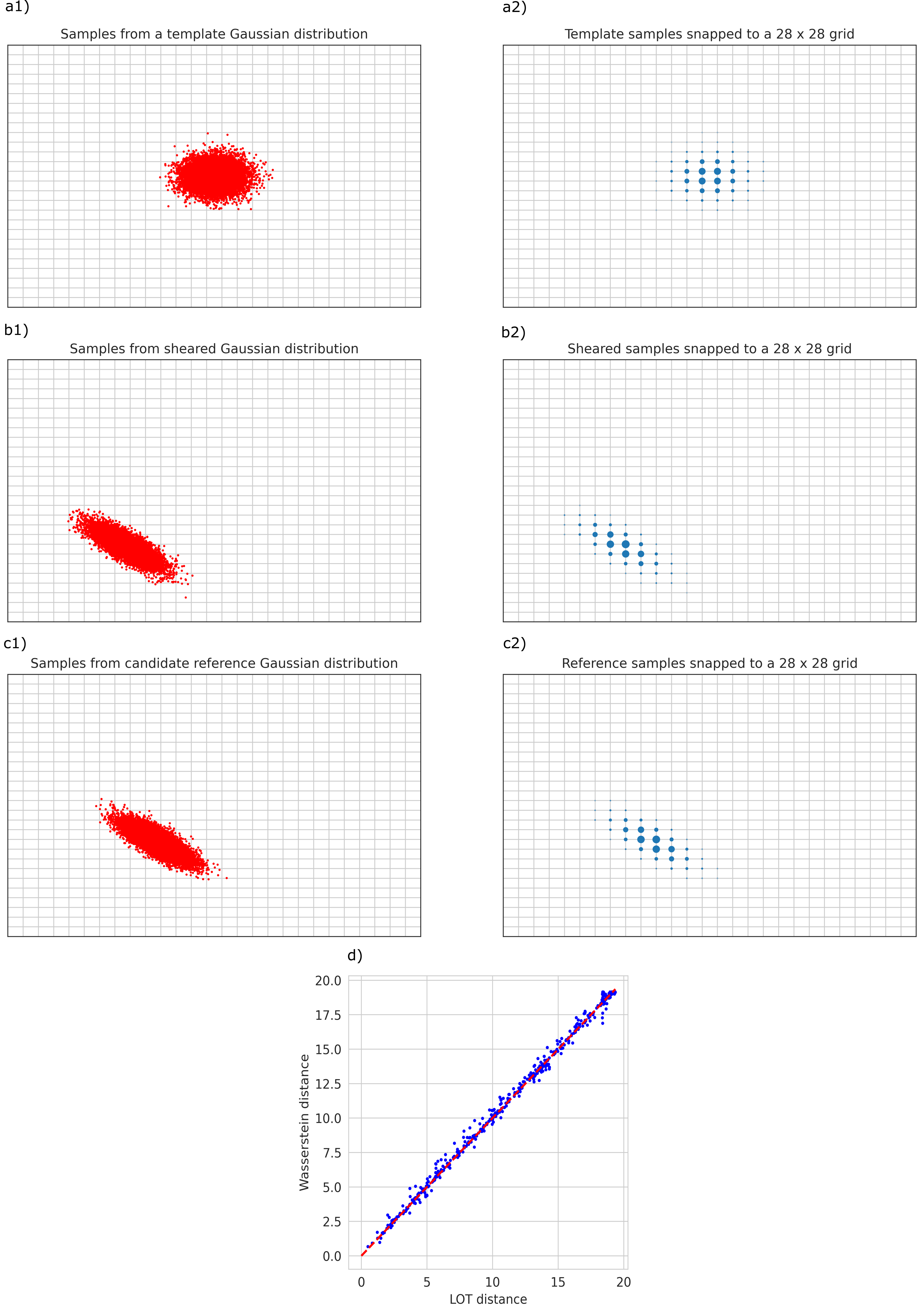
σ=𝒩⁡(C​m1+d,C​C⊤)=𝒩⁡(C​m1+d,P⊤​D2​P).\displaystyle\sigma=\mathcal{N}(Cm_{1}+d,CC^{\top})=\mathcal{N}(Cm_{1}+d,P^{\top}D^{2}P).
Refer to caption
Figure 10: a1) Samples from a Gaussian distribution that serves as the template μ\mu. a2) Approximation of the template distribution as a discrete distribution on a grid. b1) Samples from sheared distribution S♯​μS_{\sharp}\mu. b2) Approximation of the sheared distribution as a discrete distribution on a grid. c1) Samples from a candidate referencec distribution f♯​μ∈ℱaffine​(P)f_{\sharp}\mu\in\mathcal{F}_{\text{affine}}(P) (equation 11). c2) Approximation of the reference distribution as a discrete distribution on a grid. d) Numerical validation of the equivalence of LOT distance W2,f♯​μL​O​T​(μ,S♯​μ)W_{2,f_{\sharp\mu}}^{LOT}(\mu,S_{\sharp}\mu) and the Wasserstein distance W2​(μ,S♯​μ)W_{2}(\mu,S_{\sharp}\mu) under compatibility as in example 11 using the LOT framework for different choices of shear SS.

Appendix G Comparison with Convolutional Neural Networks (CNNs)
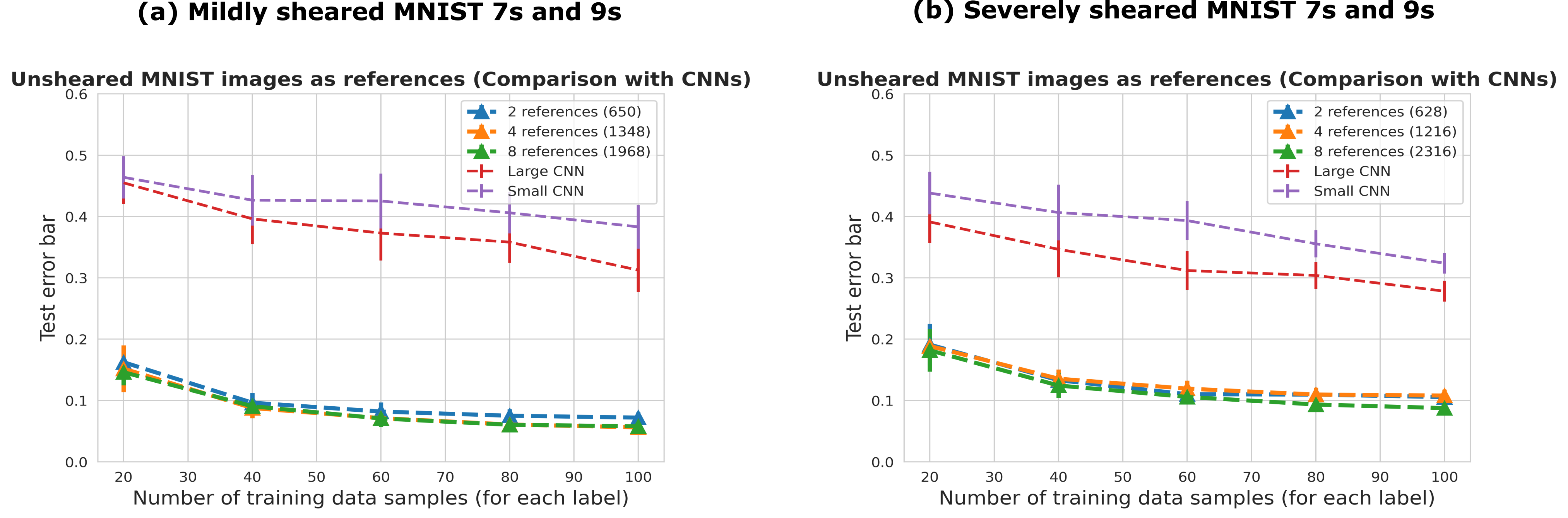
Refer to caption
Figure 11: Comparison of discrete LOT classification of (a) mildly sheared MNIST 7s and 9s (b) severely sheared MNIST 7s and 9s with convolutional neural network with 1586 training parameters (labelled small CNN) and 3650 training parameters (labelled large CNN) under identical training and testing conditions.