跳到论文正文
W Papers独立论文阅读器 arXiv:2201.10509 论文正文 计算阅读时间 · 0%
引用这篇论文根据当前论文元数据生成,正式投稿前建议核对。


License: arXiv.org perpetual non-exclusive license
arXiv:2201.10509v1 [cs.RO] 25 Jan 2022

Real-Time Deployment of a Large-Scale Multi-Quadcopter System (MQS)

Hossein Rastgoftar Thanks: H. Rastgoftar is with the Department of Aerospace and Mechanical Engineering at the University of Arizona, Tucson, AZ 85721, USA Email: hrastgoftar@arizona.edu
Abstract

This paper presents a continuum mechanics-based approach for real-time deployment (RTD) of a multi-quadcopter system between moving initial and final configurations arbitrarily distributed in a 33-D motion space. The proposed RTD problem is decomposed into spatial planning, temporal planning and acquisition sub-problems. For the spatial planning, the RTD desired coordination is defined by integrating (i) rigid-body rotation, (ii) one-dimensional homogeneous deformation, and (ii) one-dimensional heterogeneous coordination such that necessary conditions for inter-agent collision avoidance between every two quadcopter UAVs are satisfied. By the RTD temporal planning, this paper suffices the inter-agent collision avoidance between every two individual quadcopters, and assures the boundedness of the rotor angular speeds for every individual quadcopter. For the RTD acquisition, each quadcopter modeled by a nonlinear dynamics applies a nonlinear control to stably and safely track the desired RTD trajectory such that the angular speeds of each quadcopter remain bounded and do not exceed a certain upper limit.

Index Terms:
Real-Time Deployment, Nonlinear Control Design, Multi-Quadcopter System, and Multi-Agent Coordination.

I Introduction

Over the past few decades, multi-agent coordination problems have been extensively studied and found numerous applications in surveillance [1], search and rescue [2], agricultural scouting [3], structural health monitoring [4], and air traffic management [5]. Early work on multi-agent coordination commonly treats a group of vehicles (agents) as particles of a single rigid or deformable body acquiring the desired coordination in a centralized fashion through leader-less [6, 7, 8] or leader-follower communication-based [9, 10, 11, 12] approaches. More recently, researchers have studied real-time deployment (RTD) of multi-agent systems which is also called optimal mass transport (OMT) in the literature. In the OMT problem, agent coordination is governed by the continuity PDE and assigned by finding the optimal transformation between two arbitrary distributions with an equal mass [13, 14]. The existing OMT work assures convergence of agent deployment from an initial distribution to a target configuration. However, inter-agent collision avoidance may not be necessarily avoided when each individual agent represents an actual vehicle with finite size and nonlinear dynamics. This paper develops a novel continuum-mechanics-based approach for collision-free real-time deployment of multi-vehicle system coordinating between two moving formations in a three-dimensional coordination space, where each vehicle represents a quadcopter modeled by a nonlinear dynamics.

I-A Related Work

Early work on OMT was inspired by Schrodinger bridge problem [15, 16, 17] which was presented as transformation of the state density function from a reference configuration to a target configuration. Refs. [16, 15, 17] study the relation between the Schrodinger bridge problem and OMT problems. Mass transport of linear systems from an initial configuration to an arbitrary target configuration is presented as an energy minimization optimization problem in Ref. [18]. Furthermore, optimal transport of discrete-time linear systems are studied in Refs. [17, 19] where [19] uses linear quadratic Gaussian (LQG) regulation to formulate the OMT problem. This paper offers a continuum-mechanics-based solution to the OMT (RTD) problem which is inspired by the existing work on homogeneous transformation coordination of multi-agent systems presented in the author’s previous work [20, 21]. Because homogeneous transformation is an affine transformation, an nn-D homogeneous transformation coordination can be defined as a decentralized leader-follower problem with n+1n+1 that move independently and for and nn-D simplex at any time tt and followers acquiring the desired coordination through local communication.

I-B Contributions

This paper applies the principles of kinematics of continuum mechanics to define RTD problem between arbitrary moving configurations by combining (i) rigid-body rotation, (ii) 11-D homogeneous transformation, and (iii) 22-D heterogeneous coordination. This decomposition is advantageous since we can formally specify safety conditions, assure inter-agent collision avoidance, and impose the input constraints of individual vehicles in a large-scale RTD problem. In this paper, we consider RTD of a multi-quadcopter system (MQS) and define it as spatial planning, temporal planning, and acquisition sub-problems. For the spatial planning, the RTD paths are determined between two moving configurations such that necessary conditions for inter-agent collision avoidance are provided. The RTD temporal planning determines the reference trajectories of individual quadcopters verifying all safety requirements. For the RTD acquisition, a low-level feedback linearization control is designed for each quadcopter such that the desired RTD trajectories are stably tracked and rotor angular speeds of all quadcopters remain bounded.

I-C Outline

This paper is organized as follows: Preliminary notions are presented in Section II and followed by Problem Statement in Section III. The RTD is decomposed into planning and acquisition problems presented in Sections IV and V, respectively. The simulation results are presented in Section VI and followed by Conclusion in Section VII.

II Preliminaries

II-A Rigid-Body Rotation

To realize position, we define a global (an inertial) coordinate system, with base vectors 𝐞^1\hat{\mathbf{e}}_{1}, 𝐞^2\hat{\mathbf{e}}_{2}, and 𝐞^3\hat{\mathbf{e}}_{3}, and a local coordinate system with base vectors 𝐜^1\hat{\mathbf{c}}_{1}, 𝐜^2\hat{\mathbf{c}}_{2}, and 𝐜^3\hat{\mathbf{c}}_{3} that can rotate with respect to the inertial coordinate system. To characterize the rotation of the local coordinate system with respect to the global coordinate system, we first use the 3−2−13-2-1 Euler angles standard to characterize a rigid-body rotation by

𝐋Euler​(x1,x2,x3)=[Cx2​Cx3Cx2​Sx3−Sx2Sx1​Sx2​Cx3−Cx1​Sx3Sx1​Sx2​Sx3+Cx1​Cx3Sx1​Cx2Cx1​Sx2​Cx3+Sx1​Sx3Cx1​Sx2​Sx3−Sx1​Cx3Cx1​Cx2],\mathbf{L}_{\mathrm{Euler}}\left(x_{1},x_{2},x_{3}\right)=\begin{bmatrix}C_{x_{2}}C_{x_{3}}&C_{x_{2}}S_{x_{3}}&-S_{x_{2}}\\ S_{x_{1}}S_{x_{2}}C_{x_{3}}-C_{x_{1}}S_{x_{3}}&S_{x_{1}}S_{x_{2}}S_{x_{3}}+C_{x_{1}}C_{x_{3}}&S_{x_{1}}C_{x_{2}}\\ C_{x_{1}}S_{x_{2}}C_{x_{3}}+S_{x_{1}}S_{x_{3}}&C_{x_{1}}S_{x_{2}}S_{x_{3}}-S_{x_{1}}C_{x_{3}}&C_{x_{1}}C_{x_{2}}\end{bmatrix},

(1)

where x1x_{1}, x2x_{2}, and x3x_{3} are the first, second, and third Euler angles, respectively. Then, (𝐜^1,𝐜^2,𝐜^3)\left(\hat{\mathbf{c}}_{1},\hat{\mathbf{c}}_{2},\hat{\mathbf{c}}_{3}\right) are related to (𝐞^1,𝐞^2,𝐞^3)\left(\hat{\mathbf{e}}_{1},\hat{\mathbf{e}}_{2},\hat{\mathbf{e}}_{3}\right) by

𝐜^h(γ(t),μ(t))=𝐑D(t)𝐞^h,h=1,2,3,\hat{\mathbf{c}}_{h}(\gamma(t),\mu(t))=\mathbf{R}_{D}(t)\hat{\mathbf{e}}_{h},\qquad\penalty\ h=1,2,3, (2)

where rotation matrix 𝐑DT​(t)=𝐋Euler​(0,γ⁡(t),μ⁡(t))\mathbf{R}_{D}^{T}(t)=\mathbf{L}_{\mathrm{Euler}}\left(0,\gamma(t),\mu(t)\right) is given by

𝐑D​(t)=[cos⁡γ​cos⁡μcos⁡γ​sin⁡μ−sin⁡γ−sin⁡μcos⁡μ0sin⁡γ​cos⁡μsin⁡γ​sin⁡μcos⁡γ].\mathbf{R}_{D}(t)=\begin{bmatrix}\cos\gamma\cos\mu&\cos\gamma\sin\mu&-\sin\gamma\\ -\sin\mu&\cos\mu&0\\ \sin\gamma\cos\mu&\sin\gamma\sin\mu&\cos\gamma\\ \end{bmatrix}. (3)

Note that the rotation matrix 𝐑D​(t)\mathbf{R}_{D}(t) is defined based on the second and third Euler angles, where the first Euler angle is zero at any time tt.

II-B Position Notation

In this paper, we consider real-time deployment of an MQS consisting of NN quadcopters, where quadcopters’ identification numbers are defined by 𝒱={1,⋯,N}\mathcal{V}=\left\{1,\cdots,N\right\}. For every quadcopter i∈𝒱i\in\mathcal{V}, we define the global desired position denoted by 𝐩i=xi,g​𝐞^1+yi,g​𝐞^2+zi,g​𝐞^3\mathbf{p}_{i}=x_{i,g}\hat{\mathbf{e}}_{1}+y_{i,g}\hat{\mathbf{e}}_{2}+z_{i,g}\hat{\mathbf{e}}_{3} and the local desired position denoted by 𝐚i=ui​𝐜^1+vi​𝐞^2+wi​𝐞^3\mathbf{a}_{i}=u_{i}\hat{\mathbf{c}}_{1}+v_{i}\hat{\mathbf{e}}_{2}+w_{i}\hat{\mathbf{e}}_{3}, where 𝐩i​(t)\mathbf{p}_{i}(t) and 𝐚i​(t)\mathbf{a}_{i}(t) are related by

𝐩i​(t)=𝐝⁡(t)+𝐚i​(t),∀i∈𝒱,\mathbf{p}_{i}(t)=\mathbf{d}(t)+\mathbf{a}_{i}(t),\qquad\forall i\in\mathcal{V}, (4)

at time tt, where 𝐝⁡(t)=dx​(t)​𝐞^1+dy​(t)​𝐞^2+dz​(t)​𝐞^3\mathbf{d}(t)=d_{x}(t)\hat{\mathbf{e}}_{1}+d_{y}(t)\hat{\mathbf{e}}_{2}+d_{z}(t)\hat{\mathbf{e}}_{3} is the rigid-body displacement vector assigning position of the origin of the local coordinate system. The actual position of quadcopter i∈𝒱i\in\mathcal{V} is denoted by 𝐫i​(t)\mathbf{r}_{i}(t) and expressed with respect to the inertial coordinate system by 𝐫i​(t)=xi​(t)​𝐞^1+yi​(t)​𝐞^2+zi​(t)​𝐞^3\mathbf{r}_{i}(t)=x_{i}(t)\hat{\mathbf{e}}_{1}+y_{i}(t)\hat{\mathbf{e}}_{2}+z_{i}(t)\hat{\mathbf{e}}_{3}. This paper considers real-time deployment over the finite time interval [ts,tf][t_{s},t_{f}] where the initial and final local positions of every quadcopter i∈𝒱i\in\mathcal{V}, denoted by 𝐚i,s=𝐚i​(ts)\mathbf{a}_{i,s}=\mathbf{a}_{i}(t_{s}) and 𝐚i,f=𝐚i​(tf)\mathbf{a}_{i,f}=\mathbf{a}_{i}(t_{f}), are known.

Assumption 1.

We define unit vectors 𝐞^1\hat{\mathbf{e}}_{1}, 𝐞^2\hat{\mathbf{e}}_{2}, and 𝐞^3\hat{\mathbf{e}}_{3} as 𝐞^1=[100]T\hat{\mathbf{e}}_{1}=\begin{bmatrix}1&0&0\end{bmatrix}^{T}, 𝐞^2=[010]T\hat{\mathbf{e}}_{2}=\begin{bmatrix}0&1&0\end{bmatrix}^{T}, and 𝐞^3=[001]T\hat{\mathbf{e}}_{3}=\begin{bmatrix}0&0&1\end{bmatrix}^{T}. Therefore, rigid-body displacement, actual position, and global desired positions can be expressed in vector forms by 𝐝=[dxdydz]T\mathbf{d}=\begin{bmatrix}d_{x}&d_{y}&d_{z}\end{bmatrix}^{T}, 𝐫i=[xiyizi]T\mathbf{r}_{i}=\begin{bmatrix}x_{i}&y_{i}&z_{i}\end{bmatrix}^{T}, and 𝐩i=[xi,gyi,gzi,g]T\mathbf{p}_{i}=\begin{bmatrix}x_{i,g}&y_{i,g}&z_{i,g}\end{bmatrix}^{T}, respectively.

III Problem Statement

We consider an MQS consisting of NN quadcopters where dynamics of quadcopter i∈𝒱i\in\mathcal{V} is given by

{𝐱˙i=𝐟⁡(𝐱i)+𝐠⁡(𝐱i)​𝐮i𝐲i=𝐂𝐱i,∀i∈𝒱.\begin{cases}\dot{\mathbf{x}}_{i}=\mathbf{f}\left(\mathbf{x}_{i}\right)+\mathbf{g}\left(\mathbf{x}_{i}\right)\mathbf{u}_{i}\\ \mathbf{y}_{i}=\mathbf{C}\mathbf{x}_{i}\end{cases},\qquad\forall i\in\mathcal{V}. (5)

In (5), 𝐱i∈ℝ14\mathbf{x}_{i}\in\mathbb{R}^{14} is the state vector; actual position 𝐲i∈ℝ4\mathbf{y}_{i}\in\mathbb{R}^{4} is the output vector; 𝐮i∈ℝ4\mathbf{u}_{i}\in\mathbb{R}^{4} is the input vector; 𝐂∈ℝ4×14\mathbf{C}\in\mathbb{R}^{4\times 14} is constant; 𝐟:ℝ14→ℝ14\mathbf{f}:\mathbb{R}^{14}\rightarrow\mathbb{R}^{14} and 𝐠:ℝ14→ℝ14×4\mathbf{g}:\mathbb{R}^{14}\rightarrow\mathbb{R}^{14\times 4} are smooth functions; 𝐱i\mathbf{x}_{i}, 𝐮i\mathbf{u}_{i}, 𝐟\mathbf{f}, 𝐠\mathbf{g}, and 𝐂\mathbf{C} are specified in Section V. For every quadcopter i∈𝒱i\in\mathcal{V}, we define the following properties and characteristics:

  1. 1.

    Agent size ϵ\epsilon: Every quadcopter i∈𝒱i\in\mathcal{V} can be enclosed by a ball of radius ϵ\epsilon.

  2. 2.

    Deviation upper bound δ\delta: This paper assumes that each quadcopter can execute a proper trajectory tracking control such that the norm of tracking error is less than δ\delta for every quadcopter i∈𝒱i\in\mathcal{V} at any time tt.

  3. 3.

    Quadcopter rotor speed: Angular speed of rotor j∈{1,2,3,4}j\in\left\{1,2,3,4\right\} of quadcopter i∈𝒱i\in\mathcal{V} is denoted by ϖi​j\varpi_{ij}. The rotor angular speeds cannot exceed the upper bound ϖmax\varpi_{\mathrm{max}} for every quadcopter i∈𝒱i\in\mathcal{V}.

  4. 4.

    Admissible control set 𝒰\mathcal{U}: Control input 𝐮i\mathbf{u}_{i}, executed by quadcopter i∈𝒱i\in\mathcal{V}, must belong to compact set 𝒰\mathcal{U}, i.e. ui∈𝒰,∀i∈𝒱u_{i}\in\mathcal{U},\penalty\ \forall i\in\mathcal{V}.

We assume that the initial and final configurations of the quadcopter team are arbitrarily distributed in the motion space and defined by sets

Ωs={𝐚i,s=ui,s𝐜^1,s+vi,s𝐜^2,s+wi,s𝐜^3,s,∀i∈𝒱},\Omega_{s}=\left\{\mathbf{a}_{i,s}=u_{i,s}\hat{\mathbf{c}}_{1,s}+v_{i,s}\hat{\mathbf{c}}_{2,s}+w_{i,s}\hat{\mathbf{c}}_{3,s},\penalty\ \forall i\in\mathcal{V}\right\}, (6a)
Ωf={𝐚i,f=ui,f𝐜^1,f+vi,f𝐜^2,f+wi,f𝐜^3,f,∀i∈𝒱},\Omega_{f}=\left\{\mathbf{a}_{i,f}=u_{i,f}\hat{\mathbf{c}}_{1,f}+v_{i,f}\hat{\mathbf{c}}_{2,f}+w_{i,f}\hat{\mathbf{c}}_{3,f},\penalty\ \forall i\in\mathcal{V}\right\}, (6b)

where

𝐚i,s=𝐚i​(ts),∀i∈𝒱,\mathbf{a}_{i,s}=\mathbf{a}_{i}(t_{s}),\qquad\forall i\in\mathcal{V}, (7a)
𝐚i,f=𝐚i​(tf),∀i∈𝒱,\mathbf{a}_{i,f}=\mathbf{a}_{i}(t_{f}),\qquad\forall i\in\mathcal{V}, (7b)
𝐜^h,s=𝐜^h(γs,μs),h=1,2,3,\hat{\mathbf{c}}_{h,s}=\hat{\mathbf{c}}_{h}\left(\gamma_{s},\mu_{s}\right),\qquad h=1,2,3, (7c)
𝐜^h,f=𝐜^h(γf,μf),h=1,2,3.\hat{\mathbf{c}}_{h,f}=\hat{\mathbf{c}}_{h}\left(\gamma_{f},\mu_{f}\right),\qquad h=1,2,3. (7d)

Note that Ωs\Omega_{s} and Ωf\Omega_{f} are expressed with respect to the local coordinate system at times tst_{s} and tft_{f}, respectively. However, γs=γ⁡(ts)\gamma_{s}=\gamma\left(t_{s}\right), μs=μ⁡(ts)\mu_{s}=\mu\left(t_{s}\right), γf=γ⁡(tf)\gamma_{f}=\gamma\left(t_{f}\right), and μf=μ⁡(tf)\mu_{f}=\mu\left(t_{f}\right) are assigned based on initial and target positions of the MQS, expressed with respect to the inertial coordinate system, by solving the following optimization problem:

(γs,μs)=arg⁡maxγ,μ∈[0,π)⁡(mini,h∈𝒱,i≠h⁡|(𝐩i,s−𝐩h,s)⋅𝐜^1​(γ,μ)|),\left(\gamma_{s},\mu_{s}\right)=\argmax\limits_{\gamma,\mu\in\left[0,\pi\right)}\left(\min\limits_{i,h\in\mathcal{V},\penalty\ i\neq h}\left|\left(\mathbf{p}_{i,s}-\mathbf{p}_{h,s}\right)\cdot\hat{\mathbf{c}}_{1}\left(\gamma,\mu\right)\right|\right), (8a)
(γf,μf)=arg⁡maxγ,μ∈[0,π)⁡(mini,h∈𝒱,i≠h⁡|(𝐩i,f−𝐩h,f)⋅𝐜^1​(γ,μ)|),\left(\gamma_{f},\mu_{f}\right)=\argmax\limits_{\gamma,\mu\in\left[0,\pi\right)}\left(\min\limits_{i,h\in\mathcal{V},\penalty\ i\neq h}\left|\left(\mathbf{p}_{i,f}-\mathbf{p}_{h,f}\right)\cdot\hat{\mathbf{c}}_{1}\left(\gamma,\mu\right)\right|\right), (8b)

where “⋅\cdot” is the dot product symbol. Eqs. (8a) and (8b) assign (γs,μs)\left(\gamma_{s},\mu_{s}\right) and (γf,μf)\left(\gamma_{f},\mu_{f}\right) such that the minimum separation distance along unit vector 𝐜^1\hat{\mathbf{c}}_{1} is maximized.

Given above problem setting, the main objective of this paper is to define desired deployment trajectory 𝐩i​(t)\mathbf{p}_{i}(t) and choose 𝐮i​(t)\mathbf{u}_{i}(t), for every quadcopter i∈𝒱i\in\mathcal{V}, such that initial condition (7a), final condition (7b), and the following safety conditions are all satisfied:

⋀i∈𝒱⋀j=14(|ϖi​j​(t)|≤ϖmax),∀t∈[ts,tf],\bigwedge_{i\in\mathcal{V}}\bigwedge_{j=1}^{4}\left(\left|\varpi_{ij}(t)\right|\leq\varpi_{\mathrm{max}}\right),\qquad\forall t\in\left[t_{s},t_{f}\right], (9a)
⋀i=1N−1⋀j=i+1N(‖𝐫i​(t)−𝐫j​(t)‖≥2​ϵ),∀t∈[ts,tf],\bigwedge_{i=1}^{N-1}\bigwedge_{j=i+1}^{N}\left(\|\mathbf{r}_{i}(t)-\mathbf{r}_{j}(t)\|\geq 2\epsilon\right),\qquad\forall t\in\left[t_{s},t_{f}\right], (9b)
⋀i∈𝒱(‖𝐫i​(t)−𝐩i​(t)‖≤δ),∀t∈[ts,tf].\bigwedge_{i\in\mathcal{V}}\left(\|\mathbf{r}_{i}(t)-\mathbf{p}_{i}(t)\|\leq\delta\right),\qquad\forall t\in\left[t_{s},t_{f}\right]. (9c)

Condition (9a) assures that the angular speed of no rotor exceeds ϖmax\varpi_{\mathrm{max}}. Eq. (9b) specifies the inter-agent avoidance collision between every two quadcopters. Stable tracking condition is formally specified by Eq. (9c).

To assign 𝐩i​(t)\mathbf{p}_{i}(t), for every quadcopter i∈𝒱i\in\mathcal{V}, deployment of the MQS–from arbitrary initial Ωs{\Omega}_{s} to target configuration Ωf{\Omega}_{f}–is defined by integrating three collective motion modes: (i) rigid-body rotation, (ii) homogeneous ccordination, and (iii) heterogeneous coordination. Assuming every quadcopter can satisfy safety condition (9c), Section IV provides guarantee conditions for inter-agent collision avoidance in a large-scale RTD. The RTD planning is complemented with the RTD acquisition in Section V where we apply a feedback linearization approach to design control 𝐮i\mathbf{u}_{i}, for every quadcopter i∈𝒱i\in\mathcal{V}, such that: (i) quadcopter i∈𝒱i\in\mathcal{V} stably tracks the desired trajectory 𝐩i​(t)\mathbf{p}_{i}(t) and safety conditions (9a) and (9c) are both satisfied.

IV RTD Planning

Given the initial and final condition (7a) and (7b), the desired position of quadcopter i∈𝒱i\in\mathcal{V}, denoted by

𝐚i​(t)=ui​(t)​𝐜^1​(γ⁡(t),μ⁡(t))+vi​(t)​𝐜^2​(γ⁡(t),μ⁡(t))+wi​(t)​𝐜^3​(γ⁡(t),μ⁡(t)),\begin{split}\mathbf{a}_{i}(t)=&u_{i}(t)\hat{\mathbf{c}}_{1}\left(\gamma(t),\mu(t)\right)+v_{i}(t)\hat{\mathbf{c}}_{2}\left(\gamma(t),\mu(t)\right)\\ +&w_{i}(t)\hat{\mathbf{c}}_{3}\left(\gamma(t),\mu(t)\right),\end{split} (10)

is planned under the assumption that the the desired formation of the MQS translates rigidly with constant velocities at the initial time tst_{s} and final time tft_{f}. This assumption can be satisfied, if:

𝐚˙i​(ts)=𝐚˙i​(tf)=0,∀i∈𝒱,\dot{\mathbf{a}}_{i}\left(t_{s}\right)=\dot{\mathbf{a}}_{i}\left(t_{f}\right)=0,\qquad\forall i\in\mathcal{V}, (11a)
𝐚¨i​(ts)=𝐚¨i​(tf)=0,∀i∈𝒱.\ddot{\mathbf{a}}_{i}\left(t_{s}\right)=\ddot{\mathbf{a}}_{i}\left(t_{f}\right)=0,\qquad\forall i\in\mathcal{V}. (11b)

Therefore, the global desired velocities of the quadcopters satisfy the following initial and final conditions:

𝐩˙i​(t)=𝐝˙​(ts)=constant,∀i∈𝒱,t≤ts,\dot{\mathbf{p}}_{i}\left(t\right)=\dot{\mathbf{d}}\left(t_{s}\right)=\mathrm{constant},\qquad\forall i\in\mathcal{V},\penalty\ t\leq t_{s}, (12a)
𝐩˙i​(tf)=𝐝˙​(tf)=constant,∀i∈𝒱,t≥tf.\dot{\mathbf{p}}_{i}\left(t_{f}\right)=\dot{\mathbf{d}}\left(t_{f}\right)=\mathrm{constant},\qquad\forall i\in\mathcal{V},\penalty\ t\geq t_{f}. (12b)

The RTD problem is spatially planned by combining three collective motion modes: (i) rigid-body rotation, (ii) homogeneous motion along 𝐜^1\hat{\mathbf{c}}_{1}, and (iii) heterogeneous motion in 𝐜^2−𝐜^3\hat{\mathbf{c}}_{2}-\hat{\mathbf{c}}_{3} plane.

In Sections IV-A, IV-B, and IV-C, we use the quintic polynomial function

σ⁡(t,ts,tf)=15​(t−tstf−ts)5−16​(t−tstf−ts)4+10​(t−tstf−ts)3,\sigma(t,t_{s},t_{f})=15\left({t-t_{s}\over t_{f}-t_{s}}\right)^{5}-16\left({t-t_{s}\over t_{f}-t_{s}}\right)^{4}+10\left({t-t_{s}\over t_{f}-t_{s}}\right)^{3}, (13)

for t∈[ts,tf]t\in\left[t_{s},t_{f}\right], to define the collective motion modes in an RTD problem. Note that σ⁡(ts,ts,tf)=0\sigma(t_{s},t_{s},t_{f})=0, σ⁡(tf,ts,tf)=1\sigma(t_{f},t_{s},t_{f})=1, σ˙​(ts,ts,tf)=σ˙​(tf,ts,tf)=0\dot{\sigma}(t_{s},t_{s},t_{f})=\dot{\sigma}(t_{f},t_{s},t_{f})=0, and σ¨​(ts,ts,tf)=σ¨​(tf,ts,tf)=0\ddot{\sigma}(t_{s},t_{s},t_{f})=\ddot{\sigma}(t_{f},t_{s},t_{f})=0. Note that σ⁡(t,ts,tf)\sigma(t,t_{s},t_{f}) is strictly increasing with respect to tt.

IV-A Rigid-Body Rotation

The orientation of the local coordinate system are assigned by using (2), where rotation matrix 𝐑D​(t)\mathbf{R}_{D}(t), defined based on γ⁡(t)\gamma(t) and μ⁡(t)\mu(t) at any time t∈[ts,tf]t\in\left[t_{s},t_{f}\right], is given in (3). Therefore, rigid-body rotation of the MQS is specified by angles γ⁡(t)\gamma(t) and μ⁡(t)\mu(t) at any time t∈[ts,tf]t\in\left[t_{s},t_{f}\right]. Given (γs,μs)\left(\gamma_{s},\mu_{s}\right) and (γf,μf)\left(\gamma_{f},\mu_{f}\right), we define

γ⁡(t)=γs​(1−σ⁡(t,ts,tf))+γf​σ​(t,ts,tf),\gamma(t)=\gamma_{s}\left(1-\sigma(t,t_{s},t_{f})\right)+\gamma_{f}\sigma(t,t_{s},t_{f}), (14a)
μ⁡(t)=μs​(1−σ⁡(t,ts,tf))+μf​σ​(t,ts,tf),\mu(t)=\mu_{s}\left(1-\sigma(t,t_{s},t_{f})\right)+\mu_{f}\sigma(t,t_{s},t_{f}), (14b)

for t∈[ts,tf]t\in\left[t_{s},t_{f}\right].

Refer to caption
Refer to caption
Refer to caption
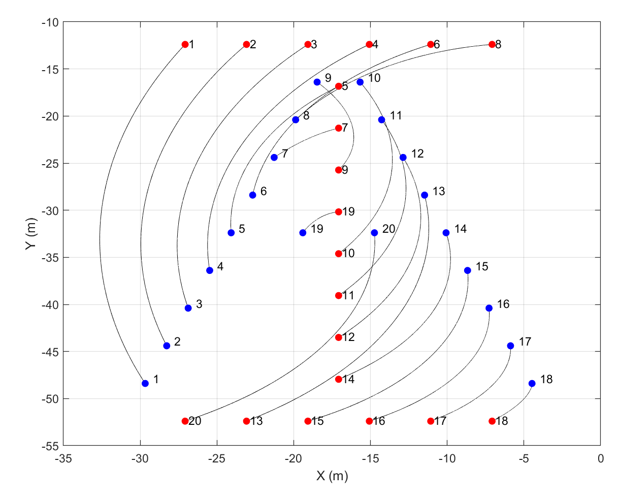
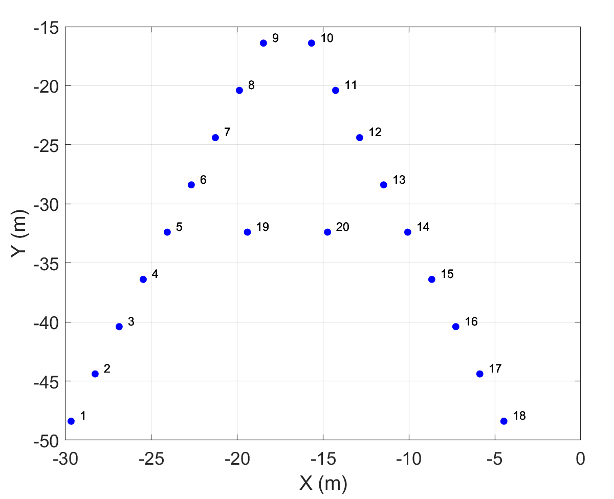
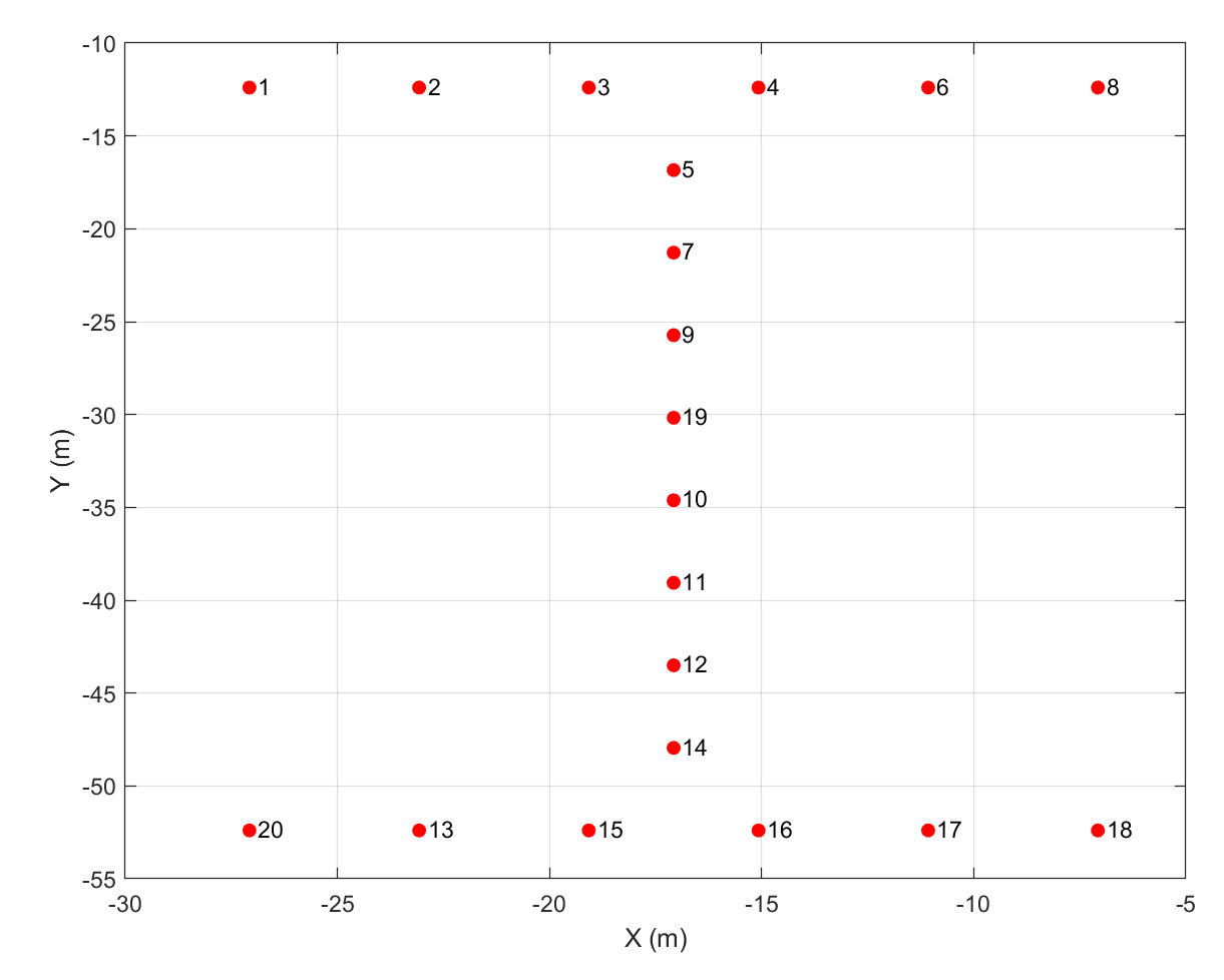
Figure 1: (a) RTD paths from “A” to “I” by 20 quadcopters distributed in the x−yx-y plane, i.e γ⁡(t)=0\gamma(t)=0 at any time t∈[ts,tf]t\in\left[t_{s},t_{f}\right]. (b) Initial formation (Letter “A”): μs=μ⁡(ts)=172.8​deg\mu_{s}=\mu\left(t_{s}\right)=172.8\deg, b1=18b_{1}=18, b2=17b_{2}=17, b3=16b_{3}=16, b4=15b_{4}=15, b5=14b_{5}=14, b6=13b_{6}=13, b7=12b_{7}=12, b8=20b_{8}=20, b9=11b_{9}=11, b10=10b_{10}=10, b11=19b_{11}=19, b12=9b_{12}=9, b13=8b_{13}=8, b14=7b_{14}=7, b15=6b_{15}=6, b16=5b_{16}=5, b17=4b_{17}=4, b18=3b_{18}=3, b19=2b_{19}=2, b20=1b_{20}=1. (c) Final formation (Letter “I”): μf=μ⁡(tf)=28.8​deg\mu_{f}=\mu\left(t_{f}\right)=28.8\deg.

IV-B Homogeneous Transformation Coordination along 𝐜^1\hat{\mathbf{c}}_{1}

Given angles (γs,μs)\left(\gamma_{s},\mu_{s}\right) and (γf,μf)\left(\gamma_{f},\mu_{f}\right), assigned by solving (8a) and (8b), the initial and final configurations of the UAVs, denoted by Ωs\Omega_{s} and Ωf\Omega_{f}, are given by (6a) and (6b), respectively. UAVs can be sorted based on their ui,su_{i,s} coordinates, along the unit vector 𝐜^1,s\hat{\mathbf{c}}_{1,s}, and set 𝒱\mathcal{V} be expressed by

𝒱={b1,⋯,bN:ubk,s<ubk+1,s,k=1,⋯,N−1}.\mathcal{V}=\left\{b_{1},\cdots,b_{N}:u_{b_{k},s}<u_{b_{k+1},s},\penalty\ k=1,\cdots,N-1\right\}. (15)

where bk∈𝒱b_{k}\in\mathcal{V} represents a quadcopter whose order number is kk in the initial formation Ωs{\Omega}_{s}. To assure inter-agent collision avoidance, we require that the order numbers of the quadcopters do not change when they are transforming from Ωs{\Omega}_{s} to Ωf{\Omega}_{f}. Therefore, the RTD planning satisfies the following requirement:

⋀k=1N−1(ubk​(t)<ubk+1​(t)),∀t∈[ts,tf],𝒱={b1,⋯,bN}.\bigwedge_{k=1}^{N-1}\left(u_{b_{k}}(t)<u_{b_{k+1}}(t)\right),\qquad\forall t\in\left[t_{s},t_{f}\right],\penalty\ \mathcal{V}=\left\{b_{1},\cdots,b_{N}\right\}. (16)

Per this requirement, the order numbers of the quadcopters in final configuration are the same as the order numbers of quadcopters in the initial configuration. Therefore, set 𝒱\mathcal{V} can be also defined as follows:

𝒱={b1,⋯,bN:ubk,f<ubk+1,f,k=1,⋯,N−1},\mathcal{V}=\left\{b_{1},\cdots,b_{N}:u_{b_{k},f}<u_{b_{k+1},f},\penalty\ k=1,\cdots,N-1\right\}, (17)

where ubk,f=ubk​(tf)u_{b_{k},f}=u_{b_{k}}(t_{f}).

Definition 1.

Set 𝒱\mathcal{V} can be expressed as 𝒱=ℒ​⋃ℱ\mathcal{V}=\mathcal{L}\bigcup\mathcal{F} where disjoint subsets

ℒ={b1,bN},\mathcal{L}=\left\{b_{1},b_{N}\right\}, (18a)
ℱ={b2,⋯,bN−1},\mathcal{F}=\left\{b_{2},\cdots,b_{N-1}\right\}, (18b)

define the leader quadcopters and follower quadcopters, respectively.

For better clarification, consider the RTD example shown in Fig. 1 that illustrates safe coordination of 2020 quadcopters from “A” (initial formation) to “I” (final formation) in the x−yx-y plane. Because the MQS is restricted to move in the x−yx-y plane, γ⁡(t)=0\gamma(t)=0 at any time t∈[ts,tf]t\in\left[t_{s},t_{f}\right]. Given initial formation of the MQS, we obtain μs=172.8​deg\mu_{s}=172.8\deg, ℒ={18,1}\mathcal{L}=\left\{18,1\right\} (b1=18b_{1}=18, b20=1b_{20}=1) and ℱ={1,⋯,20}∖ℒ\mathcal{F}=\left\{1,\cdots,20\right\}\setminus\mathcal{L}. Given the MQS final formation (“I”), μf=28.8​deg\mu_{f}=28.8\deg is obtained.

Definition 2.

Given initial and final configurations of the MQS, we define initial reference weight βi,s\beta_{i,s} and final reference weight βi,f\beta_{i,f} for every quadcopter i∈𝒱i\in\mathcal{V} by

βi,s=ubN,s−ui,subN,s−ub1,s∈[0,1],\beta_{i,s}={u_{b_{N},s}-u_{i,s}\over u_{b_{N},s}-u_{b_{1},s}}\in\left[0,1\right], (19a)
βi,f=ubN,f−ui,subN,f−ub1,f∈[0,1].\beta_{i,f}={u_{b_{N},f}-u_{i,s}\over u_{b_{N},f}-u_{b_{1},f}}\in\left[0,1\right]. (19b)

Per definitions of set ℱ\mathcal{F}, ub1,s<ui,s<ubN,su_{b_{1},s}<u_{i,s}<u_{b_{N},s} and ub1,f<ui,f<ubN,fu_{b_{1},f}<u_{i,f}<u_{b_{N},f}. Therefore, βi,s>0\beta_{i,s}>0 and βi,f>0\beta_{i,f}>0 for every quadcopter i∈ℱi\in\mathcal{F}. Theorem 1 provides guarantee conditions for satisfaction of (16) through specifying initial and final MQS arrangements.

Theorem 1.

Define

dmin=min⁡{ubN,s−ub1,s,ubN,f−ub1,s}d_{\mathrm{min}}=\min\left\{u_{b_{N},s}-u_{b_{1},s},u_{b_{N},f}-u_{b_{1},s}\right\} (20a)
β∗=mini,j∈𝒱,i≠j⁡min⁡{|βi​j,s|,|βi​j,f|},\beta^{*}=\min\limits_{i,j\in\mathcal{V},\penalty\ i\neq j}\min\left\{\left|\beta_{ij,s}\right|,\left|\beta_{ij,f}\right|\right\}, (20b)

where

βi​j,s=βi,s−βj,s,\beta_{ij,s}=\beta_{i,s}-\beta_{j,s}, (21a)
βi​j,f=βi,f−βj,f.\beta_{ij,f}=\beta_{i,f}-\beta_{j,f}. (21b)

Assume every quadcopter i∈𝒱i\in\mathcal{V} can execute a proper control input 𝐮i\mathbf{u}_{i} such that safety condition (9c) is satisfied when every quadcopter is enclosed by a ball of radius ϵ\epsilon. Then, inter-agent collision avoidance between every two quadcopters are avoided, if

dmin​β∗≥2​(δ+ϵ),d_{\mathrm{min}}\beta^{*}\geq 2\left(\delta+\epsilon\right), (22)

and the uiu_{i} component of local desired position of every quadcopter i∈𝒱i\in\mathcal{V} is defined by

ui​(t)={(1−σ⁡(t,ts,tf))​ui,s+σ⁡(t,ts,tf)​ui,fi∈ℒ(1−βi​(t))​ub1​(t)+βi​(t)​ubN​(t)i∈ℱu_{i}(t)=\begin{cases}\left(1-\sigma\left(t,t_{s},t_{f}\right)\right)u_{i,s}+\sigma\left(t,t_{s},t_{f}\right)u_{i,f}&i\in\mathcal{L}\\ \left(1-\beta_{i}\left(t\right)\right)u_{b_{1}}\left(t\right)+\beta_{i}\left(t\right)u_{b_{N}}\left(t\right)&i\in\mathcal{F}\\ \end{cases} (23)

at any time t∈[ts,tf]t\in\left[t_{s},t_{f}\right], where

βi​(t)=(1−σ⁡(t,ts,tf))​βi,s+σ⁡(t,ts,tf)​βi,f,∀i∈𝒱.\beta_{i}(t)=\left(1-\sigma\left(t,t_{s},t_{f}\right)\right)\beta_{i,s}+\sigma\left(t,t_{s},t_{f}\right)\beta_{i,f},\qquad\forall i\in\mathcal{V}. (24)
Proof.

Quadcopters ii and jj can both be enclosed by two balls with the same radius ϵ\epsilon but different centers located at 𝐫i​(t)\mathbf{r}_{i}(t) and 𝐫j​(t)\mathbf{r}_{j}(t) (𝐫i​(t)\mathbf{r}_{i}(t) and 𝐫j​(t)\mathbf{r}_{j}(t) are the actual position of quadcopters ii and jj at time tt). If safety conditions (9c), inter-agent collision avoidance can be assured by satisfying the following condition:

⋀i=1N−1⋀j=i+1N(|ui​(t)−uj​(t)|≤2​(δ+ϵ)),∀t∈[ts,tf].\bigwedge_{i=1}^{N-1}\bigwedge_{j=i+1}^{N}\left(\left|u_{i}(t)-u_{j}(t)\right|\leq 2\left(\delta+\epsilon\right)\right),\qquad\forall t\in\left[t_{s},t_{f}\right]. (25)

When uiu_{i} and uju_{j} coordinates of different quadcopters ii and jj are defined by (23), the following relation holds:

ui​(t)−uj​(t)=(βi​(t)−βj​(t))​(ubN​(t)−ub1​(t)).u_{i}(t)-u_{j}(t)=\left(\beta_{i}(t)-\beta_{j}(t)\right)\left(u_{b_{N}}(t)-u_{b_{1}}(t)\right). (26)

Per Eq. (24), βi=(1−σ)​βi,s+σ​βi,f\beta_{i}=\left(1-\sigma\right)\beta_{i,s}+\sigma\beta_{i,f} and βj=(1−σ)​βj,s+σ​βj,f\beta_{j}=\left(1-\sigma\right)\beta_{j,s}+\sigma\beta_{j,f} can be substituted into Eq. (26); Eq. (24) can be rewritten as follows:

ui​(t)−uj​(t)=(βi​j,s+σ⁡(t,ts,tf)​(βi​j,f−βi​j,s))​(ubN​(t)−ub1​(t)).u_{i}(t)-u_{j}(t)=\left(\beta_{ij,s}+\sigma\left(t,t_{s},t_{f}\right)\left(\beta_{ij,f}-\beta_{ij,s}\right)\right)\left(u_{b_{N}}(t)-u_{b_{1}}(t)\right).

(27)

Because σ⁡(t,ts,tf)\sigma\left(t,t_{s},t_{f}\right) is strictly increasing over [ts,tf]\left[t_{s},t_{f}\right], the right-hand side of Eq. (27) reaches its minimum value, over [ts,tf]\left[t_{s},t_{f}\right], either t=tst=t_{s}, when σ=0\sigma=0, or t=tft=t_{f}, when σ=1\sigma=1:

mint∈[ts,tf]⁡|βi​j,s+σ⁡(t,ts,tf)​(βi​j,f−βi​j,s)|=min⁡{|βi​j,s|,|βi​j,f|}=β∗,\min\limits_{t\in\left[t_{s},t_{f}\right]}\left|\beta_{ij,s}+\sigma\left(t,t_{s},t_{f}\right)\left(\beta_{ij,f}-\beta_{ij,s}\right)\right|=\min\left\{\left|\beta_{ij,s}\right|,\left|\beta_{ij,f}\right|\right\}=\beta^{*},

mint∈[ts,tf]⁡(ubN​(t)−ub1​(t))=min⁡{ubN,f−ub1,f,ubN,s−ub1,s}=dmin.\min\limits_{t\in\left[t_{s},t_{f}\right]}\left(u_{b_{N}}(t)-u_{b_{1}}(t)\right)=\min\left\{u_{b_{N},f}-u_{b_{1},f},u_{b_{N},s}-u_{b_{1},s}\right\}=d_{\mathrm{min}}.

This implies that

mint∈[ts,tf](ui(t)−uj(t))≥dminβ∗,i≠j,i,j∈𝒱.\min\limits_{t\in\left[t_{s},t_{f}\right]}\left(u_{i}(t)-u_{j}(t)\right)\geq d_{\mathrm{\min}}\beta^{*},\qquad i\neq j,\penalty\ i,j\in\mathcal{V}.

Therefore, inter-agent collision avoidance (25) is satisfied, if condition (22) holds.

∎

IV-C Heterogeneous Transformation Coordination in the 𝐜^2−𝐜^3\hat{\mathbf{c}}_{2}-\hat{\mathbf{c}}_{3}

Evolution of the UAVs in the plane made by 𝐜^2\hat{\mathbf{c}}_{2} and 𝐜^2\hat{\mathbf{c}}_{2} are defined by

[vi​(t)wi​(t)]=(1−σ⁡(t,ts,tf))​[vi,swi,s]+σ⁡(t,ts,tf)​[vi,fwi,f],∀t∈[ts,tf].\begin{bmatrix}v_{i}(t)\\ w_{i}(t)\\ \end{bmatrix}=\left(1-\sigma(t,t_{s},t_{f})\right)\begin{bmatrix}v_{i,s}\\ w_{i,s}\\ \end{bmatrix}+\sigma(t,t_{s},t_{f})\begin{bmatrix}v_{i,f}\\ w_{i,f}\\ \end{bmatrix},\qquad\forall t\in\left[t_{s},t_{f}\right].

(28)

V RTD Acquisition

We first present the quadcopter dynamics in Section (V-A). Then, we design a feedback linearization control in Section V-C so that every quadcopter ii can stably track the desired RTD trajectory 𝐩i​(t)\mathbf{p}_{i}(t) and safety conditions (9a)-(9c) are all satisfied.

V-A Quadcopter Dynamics

This paper models quadcopter i∈𝒱i\in\mathcal{V} by dynamics (5) with the state vector 𝐱i\mathbf{x}_{i} and input vector 𝐮i\mathbf{u}_{i}, and smooth functions 𝐟\mathbf{f} and 𝐠\mathbf{g} defined as follows:

𝐱i=[xiyizix˙iy˙iz˙iϕiθiψiϕ˙iθ˙iψ˙ipip˙i]T,\mathbf{x}_{i}=\begin{bmatrix}x_{i}&y_{i}&z_{i}&\dot{x}_{i}&\dot{y}_{i}&\dot{z}_{i}&\phi_{i}&\theta_{i}&\psi_{i}&\dot{\phi}_{i}&\dot{\theta}_{i}&\dot{\psi}_{i}&p_{i}&\dot{p}_{i}\end{bmatrix}^{T},

(29a)
𝐮i=[up,iuϕ,iuθ,iuψ,i]T,\mathbf{u}_{i}=\begin{bmatrix}u_{p,i}&u_{\phi,i}&u_{\theta,i}&u_{\psi,i}\end{bmatrix}^{T}, (29b)
𝐟⁡(𝐱i)=[𝐫˙iT(pimi​𝐤^b,i−g​𝐞^3)Tϕ˙iθ˙iψ˙i𝟎1×3p˙i0]T,\mathbf{f}\left(\mathbf{x}_{i}\right)=\begin{bmatrix}\dot{\mathbf{r}}_{i}^{T}&\left({p_{i}\over m_{i}}\hat{\mathbf{k}}_{b,i}-g\hat{\mathbf{e}}_{3}\right)^{T}&\dot{\phi}_{i}&\dot{\theta}_{i}&\dot{\psi}_{i}&\mathbf{0}_{1\times 3}&\dot{p}_{i}&0\end{bmatrix}^{T}, (29c)
𝐠⁡(𝐱i)=[𝟎9×1𝟎9×3𝟎3×1𝐈30𝟎1×31𝟎1×3],{\mathbf{g}}\left({\mathbf{x}}_{i}\right)=\begin{bmatrix}\mathbf{0}_{9\times 1}&\mathbf{0}_{9\times 3}\\ \mathbf{0}_{3\times 1}&\mathbf{I}_{3}\\ 0&\mathbf{0}_{1\times 3}\\ 1&\mathbf{0}_{1\times 3}\\ \end{bmatrix}, (29d)
𝐂=[𝐈3𝟎3×5𝟎3×1𝟎3×5𝟎1×3𝟎1×51𝟎1×5],\mathbf{C}=\begin{bmatrix}\mathbf{I}_{3}&\mathbf{0}_{3\times 5}&\mathbf{0}_{3\times 1}&\mathbf{0}_{3\times 5}\\ \mathbf{0}_{1\times 3}&\mathbf{0}_{1\times 5}&1&\mathbf{0}_{1\times 5}\end{bmatrix}, (29e)

where 𝐫i=[xiyizi]T\mathbf{r}_{i}=\begin{bmatrix}x_{i}&y_{i}&z_{i}\end{bmatrix}^{T} is the actual position of quadcopter i∈𝒱i\in\mathcal{V}; ϕi\phi_{i}, θi\theta_{i}, and ψi\psi_{i} are the roll, pitch, and yaw angles of quadcopter i∈𝒱i\in\mathcal{V}; pip_{i} is the magnitude of the thrust force of quadcopter i∈𝒱i\in\mathcal{V}; mim_{i} is the mass of quadcopter i∈𝒱i\in\mathcal{V}, and g=9.81​m/s2g=9.81m/s^{2} is the gravity acceleration. Also, unit 𝐤^b,i\hat{\mathbf{k}}_{b,i} is the unit vector assigning the direction of the thrust force of quadcopter i∈𝒱i\in\mathcal{V}.

Refer to caption
Figure 2: Determination of rotation of quadcopter i∈𝒱i\in\mathcal{V} using the 3−2−13-2-1 standard with roll angle ϕi\phi_{i}, pitch angle θi\theta_{i}, and yaw angle ψi\psi_{i}.

V-A1 Quadcopters’ Angular Velocities and Accelerations

We use 3-2-1 standard to determine orientation of quadcopter i∈𝒱i\in\mathcal{V} at time tt with the three rotations shown in Fig. 2. Given roll angle ϕi​(t)\phi_{i}(t), pitch angle θi​(t)\theta_{i}(t), and yaw angle ψi​(t)\psi_{i}(t) and the base vectors of the inertial coordinate system (𝐞^1\hat{\mathbf{e}}_{1}, 𝐞^2\hat{\mathbf{e}}_{2}, and 𝐞^3\hat{\mathbf{e}}_{3}), we obtain (𝐢^1,i,𝐣^1,i,𝐤^1,i)\left(\hat{\mathbf{i}}_{1,i},\hat{\mathbf{j}}_{1,i},\hat{\mathbf{k}}_{1,i}\right), (𝐢^2,i,𝐣^2,i,𝐤^2,i)\left(\hat{\mathbf{i}}_{2,i},\hat{\mathbf{j}}_{2,i},\hat{\mathbf{k}}_{2,i}\right), and (𝐢^b,i,𝐣^b,i,𝐤^b,i)\left(\hat{\mathbf{i}}_{b,i},\hat{\mathbf{j}}_{b,i},\hat{\mathbf{k}}_{b,i}\right) as follows:

𝐢^1,i=𝐋EulerT​(0,0,ψi)​𝐞^1=[CΨiSψi0]T,\hat{\mathbf{i}}_{1,i}=\mathbf{L}_{\mathrm{Euler}}^{T}\left(0,0,\psi_{i}\right)\hat{\mathbf{e}}_{1}=\begin{bmatrix}C_{\Psi_{i}}&S_{\psi_{i}}&0\end{bmatrix}^{T}, (30a)
𝐣^1,i=𝐋EulerT​(0,0,ψi)​𝐞^2=[−SΨiCψi0]T,\hat{\mathbf{j}}_{1,i}=\mathbf{L}_{\mathrm{Euler}}^{T}\left(0,0,\psi_{i}\right)\hat{\mathbf{e}}_{2}=\begin{bmatrix}-S_{\Psi_{i}}&C_{\psi_{i}}&0\end{bmatrix}^{T}, (30b)
𝐤^1,i=𝐋EulerT​(0,0,ψi)​𝐞^3=[001]T,\hat{\mathbf{k}}_{1,i}=\mathbf{L}_{\mathrm{Euler}}^{T}\left(0,0,\psi_{i}\right)\hat{\mathbf{e}}_{3}=\begin{bmatrix}0&0&1\end{bmatrix}^{T}, (30c)
𝐢^2,i=𝐋EulerT​(0,θi,ψi)​𝐞^1=[Cθi​CψiCθi​Sψi−Sθi]T,\begin{split}\hat{\mathbf{i}}_{2,i}&=\mathbf{L}_{\mathrm{Euler}}^{T}\left(0,\theta_{i},\psi_{i}\right)\hat{\mathbf{e}}_{1}=\begin{bmatrix}C_{\theta_{i}}C_{\psi_{i}}&C_{\theta_{i}}S_{\psi_{i}}&-S_{\theta_{i}}\end{bmatrix}^{T},\end{split} (31a)
𝐣^2,i=𝐋EulerT​(0,θi,ψi)​𝐞^2=[−SψiCψi0]T,\begin{split}\hat{\mathbf{j}}_{2,i}&=\mathbf{L}_{\mathrm{Euler}}^{T}\left(0,\theta_{i},\psi_{i}\right)\hat{\mathbf{e}}_{2}=\begin{bmatrix}-S_{\psi_{i}}&C_{\psi_{i}}&0\end{bmatrix}^{T},\end{split} (31b)
𝐤^2,i=𝐋EulerT​(0,θi,ψi)​𝐞^3=[Sθi​CψiSθi​SψiCθi]T,\begin{split}\hat{\mathbf{k}}_{2,i}&=\mathbf{L}_{\mathrm{Euler}}^{T}\left(0,\theta_{i},\psi_{i}\right)\hat{\mathbf{e}}_{3}=\begin{bmatrix}S_{\theta_{i}}C_{\psi_{i}}&S_{\theta_{i}}S_{\psi_{i}}&C_{\theta_{i}}\end{bmatrix}^{T},\end{split} (31c)
𝐢^b,i=𝐋EulerT​(ϕi,θi,ψi)​𝐞^1=[Cθi​CψiCθi​Sψi−Sθi]T,\hat{\mathbf{i}}_{b,i}=\mathbf{L}_{\mathrm{Euler}}^{T}\left(\phi_{i},\theta_{i},\psi_{i}\right)\hat{\mathbf{e}}_{1}=\begin{bmatrix}C_{\theta_{i}}C_{\psi_{i}}&C_{\theta_{i}}S_{\psi_{i}}&-S_{\theta_{i}}\end{bmatrix}^{T}, (32a)
𝐣^b,i=𝐋EulerT​(ϕi,θi,ψi)​𝐞^2=[Cψi​Sϕi​Sθi−Cϕi​SψiCϕi​Cψi+Sϕi​Sψi​SθiCθi​Sϕi]T,\begin{split}\hat{\mathbf{j}}_{b,i}=&\mathbf{L}_{\mathrm{Euler}}^{T}\left(\phi_{i},\theta_{i},\psi_{i}\right)\hat{\mathbf{e}}_{2}\\ =&\begin{bmatrix}C_{\psi_{i}}S_{\phi_{i}}S_{\theta_{i}}-C_{\phi_{i}}S_{\psi_{i}}&C_{\phi_{i}}C_{\psi_{i}}+S_{\phi_{i}}S_{\psi_{i}}S_{\theta_{i}}&C_{\theta_{i}}S_{\phi_{i}}\end{bmatrix}^{T},\end{split} (32b)
𝐤^b,i=𝐋EulerT​(ϕi,θi,ψi)​𝐞^3=[Sϕi​Sψi+Cϕi​Cψi​SθiCϕi​Sψi​Sθi−Sϕi​CψiCϕi​Cθi]T.\begin{split}\hat{\mathbf{k}}_{b,i}=&\mathbf{L}_{\mathrm{Euler}}^{T}\left(\phi_{i},\theta_{i},\psi_{i}\right)\hat{\mathbf{e}}_{3}\\ =&\begin{bmatrix}S_{\phi_{i}}S_{\psi_{i}}+C_{\phi_{i}}C_{\psi_{i}}S_{\theta_{i}}&C_{\phi_{i}}S_{\psi_{i}}S_{\theta_{i}}-S_{\phi_{i}}C_{\psi_{i}}&C_{\phi_{i}}C_{\theta_{i}}\end{bmatrix}^{T}.\end{split} (32c)

The angular velocity of quadcopter i∈𝒱i\in\mathcal{V} is then given by

ωi=ψ˙i​𝐤^1,i+θ˙i​𝐣^2,i+ϕ˙i​𝐢^b,i.{\color[rgb]{0,0,0}\bf{\omega}}_{i}=\dot{\psi}_{i}\hat{\mathbf{k}}_{1,i}+\dot{\theta}_{i}\hat{\mathbf{j}}_{2,i}+\dot{\phi}_{i}\hat{\mathbf{i}}_{b,i}. (33)

Substituting 𝐤^1,i\hat{\mathbf{k}}_{1,i}, 𝐣^2,i\hat{\mathbf{j}}_{2,i}, and 𝐢^b,i\hat{\mathbf{i}}_{b,i} into Eq. (33), ωi=[ωx,i​ωy,i​ωz,i]T{\color[rgb]{0,0,0}{\omega}}_{i}=\left[\omega_{x,i}\penalty\ \omega_{y,i}\penalty\ \omega_{z,i}\right]^{T} is related by ϕ˙i\dot{\phi}_{i}, θ˙i\dot{\theta}_{i}, and ψ˙i\dot{\psi}_{i} by

[ωx,iωy,iωz,i]T=𝚪⁡(ϕi,θi,ψi)​[ϕ˙iθ˙iψ˙i]T,\begin{bmatrix}\omega_{x,i}&\omega_{y,i}&\omega_{z,i}\end{bmatrix}^{T}=\mathbf{\Gamma}\left(\phi_{i},\theta_{i},\psi_{i}\right)\begin{bmatrix}\dot{\phi}_{i}&\dot{\theta}_{i}&\dot{\psi}_{i}\end{bmatrix}^{T}, (34)

where

𝚪⁡(ϕi,θi,ψi)=[10−sin⁡θi0cos⁡ϕicosθisinϕi0−sin⁡ϕicosϕicosθi].\mathbf{\Gamma}\left(\phi_{i},\theta_{i},\psi_{i}\right)=\begin{bmatrix}1&0&-\sin\theta_{i}\\ 0&\cos\phi_{i}&\cos\theta_{i}\sin\phi_{i}\\ 0&-\sin\phi_{i}&\cos\phi_{i}\cos\theta_{i}\end{bmatrix}. (35)

Angular acceleration of quadcopter i∈𝒱i\in\mathcal{V} is obtained by taking the time derivative of the angular velocity vector ωi{\color[rgb]{0,0,0}\bf{\omega}}_{i} and related to control vector 𝐮i\mathbf{u}_{i} by [20]:

ω˙i=𝐁~1,i​[𝟎3×1𝐈3]​𝐮i+𝐁~2,i.\begin{split}\dot{{\color[rgb]{0,0,0}\bf{\omega}}}_{i}=\tilde{\mathbf{B}}_{1,i}\begin{bmatrix}\mathbf{0}_{3\times 1}&\mathbf{I}_{3}\end{bmatrix}\mathbf{u}_{i}+\tilde{\mathbf{B}}_{2,i}.\end{split} (36)

where

𝐁~1,i=[𝐢^b,i𝐣^2,i𝐤^1,i]\tilde{\mathbf{B}}_{1,i}=\begin{bmatrix}\hat{\mathbf{i}}_{b,i}&\hat{\mathbf{j}}_{2,i}&\hat{\mathbf{k}}_{1,i}\end{bmatrix} (37a)
𝐁~2,i=θ˙i​ψ˙i​(𝐤^1,i×𝐣^1,i)+ϕ˙i​(ψ˙i​𝐤^1,i+θ˙i​𝐣^2,i)×𝐢^2,i\tilde{\mathbf{B}}_{2,i}=\dot{\theta}_{i}\dot{\psi}_{i}\left(\hat{\mathbf{k}}_{1,i}\times\hat{\mathbf{j}}_{1,i}\right)+\dot{\phi}_{i}\left(\dot{\psi}_{i}\hat{\mathbf{k}}_{1,i}+\dot{\theta}_{i}\hat{\mathbf{j}}_{2,i}\right)\times\hat{\mathbf{i}}_{2,i} (37b)

The rotational dynamics of quadcopter i∈𝒱i\in\mathcal{V} is given by [22]

𝐉iω˙i=−ωi×(𝐉iωi)−Jr,iωi×ϖi,r𝐤^b,i+𝐓i\mathbf{J}_{i}\dot{\bf{\omega}}_{i}=-{\omega}_{i}\times\left(\mathbf{J}_{i}{\omega}_{i}\right)-{J}_{r,i}{\omega}_{i}\times\varpi_{i,r}\hat{\mathbf{k}}_{b,i}+\mathbf{T}_{i} (38)

where

𝐓i=τϕ,i​𝐢^b,i+τθ,i​𝐣^b,i+τψ,i​𝐤^b,i=𝐁~1,i​[τϕ,iτθ,iτψ,i]T\begin{split}\mathbf{T}_{i}=&\tau_{\phi,i}\hat{\mathbf{i}}_{b,i}+\tau_{\theta,i}\hat{\mathbf{j}}_{b,i}+\tau_{\psi,i}\hat{\mathbf{k}}_{b,i}=\tilde{\mathbf{B}}_{1,i}\begin{bmatrix}\tau_{\phi,i}&\tau_{\theta,i}&\tau_{\psi,i}\end{bmatrix}^{T}\end{split} (39)

is the quadcopter torque exerted on quadcopter i∈𝒱i\in\mathcal{V}.

Refer to caption
Figure 3: Schematic of the plane of quadcopter i∈𝒱i\in\mathcal{V} defined by base vectors 𝐢^b,i\hat{\mathbf{i}}_{b,i} and 𝐣^b,i\hat{\mathbf{j}}_{b,i}.

V-B Rotors’ Angular Speeds

The thrust force generated by rotor j∈{1,2,3,4}j\in\left\{1,2,3,4\right\} of quadcopter i∈𝒱i\in\mathcal{V} is denoted by pi​jp_{ij} and defined as follows:

pi​j=b​ϖi​j2,∀i∈𝒱,j∈{1,2,3,4},p_{ij}=b\varpi_{ij}^{2},\qquad\forall i\in\mathcal{V},\penalty\ j\in\left\{1,2,3,4\right\}, (40)

where b>0b>0 is the aerodynamic constant. The standard shown in Fig. 3 is used to situate motors of quadcopter i∈𝒱i\in\mathcal{V}, thus, components of torque 𝐓i\mathbf{T}_{i}, exerted on quadcopter i∈𝒱i\in\mathcal{V}, are obtained as follows:

τϕ,i=l⁡(pi​4−pi​2)=b​l​(ϖi​42−ϖi​22),∀i∈𝒱,\tau_{\phi,i}=l\left(p_{i4}-p_{i2}\right)=bl\left(\varpi_{i4}^{2}-\varpi_{i2}^{2}\right),\qquad\forall i\in\mathcal{V}, (41a)
τθ,i=l⁡(pi​3−pi​1)=b​l​(ϖi​32−ϖi​12),∀i∈𝒱,\tau_{\theta,i}=l\left(p_{i3}-p_{i1}\right)=bl\left(\varpi_{i3}^{2}-\varpi_{i1}^{2}\right),\qquad\forall i\in\mathcal{V}, (41b)
τψ,i=k​∑j=14(−1)j​ϖi​j2,∀i∈𝒱,\tau_{\psi,i}=k\sum_{j=1}^{4}(-1)^{j}\varpi_{ij}^{2},\qquad\forall i\in\mathcal{V}, (41c)

where kk is the aerodynamic constant in Eq. (41c). Therefore, the rotors’ angular speeds can be uniquely determined based on the thrust force (pip_{i}) and control torque components (τϕ,i\tau_{\phi,i}, τθ,i\tau_{\theta,i}, and τψ,i\tau_{\psi,i}) by

[piτϕ,iτθ,iτψ,i]=[bibibibi0−bi​li0bi​li−bi​li0bi​li0−kiki−kiki]​[ϖi​12ϖi​22ϖi​32ϖi​42],∀i∈𝒱.\begin{bmatrix}p_{i}\\ \tau_{\phi,i}\\ \tau_{\theta,i}\\ \tau_{\psi,i}\end{bmatrix}=\begin{bmatrix}b_{i}&b_{i}&b_{i}&b_{i}\\ 0&-b_{i}l_{i}&0&b_{i}l_{i}\\ -b_{i}l_{i}&0&b_{i}l_{i}&0\\ -k_{i}&k_{i}&-k_{i}&k_{i}\end{bmatrix}\begin{bmatrix}\varpi_{i1}^{2}\\ \varpi_{i2}^{2}\\ \varpi_{i3}^{2}\\ \varpi_{i4}^{2}\\ \end{bmatrix},\qquad\forall i\in\mathcal{V}. (42)
Proposition 1.

Given pip_{i}, ϕi\phi_{i}, θi\theta_{i}, ψi\psi_{i}, p˙i\dot{p}_{i}, ϕ˙i\dot{\phi}_{i}, θ˙i\dot{\theta}_{i}, ψ˙i\dot{\psi}_{i}, and 𝐮i=[up,iuϕ,iuθ,iuψ,i]T\mathbf{u}_{i}=\begin{bmatrix}u_{p,i}&u_{\phi,i}&u_{\theta,i}&u_{\psi,i}\end{bmatrix}^{T} at time t∈[ts,tf]t\in\left[t_{s},t_{f}\right], the angular speeds of rotors of quadcopter ii are determined by solving the following set of quadratic algebraic equations:

𝐇1,i​[ϖi​12ϖi​22ϖi​32ϖi​42]+𝐇2,i​[ϖi​1ϖi​2ϖi​3ϖi​4]+𝐇3,i=𝟎4×1,∀i∈𝒱,\mathbf{H}_{1,i}\begin{bmatrix}\varpi_{i1}^{2}\\ \varpi_{i2}^{2}\\ \varpi_{i3}^{2}\\ \varpi_{i4}^{2}\end{bmatrix}+\mathbf{H}_{2,i}\begin{bmatrix}\varpi_{i1}\\ \varpi_{i2}\\ \varpi_{i3}\\ \varpi_{i4}\\ \end{bmatrix}+\mathbf{H}_{3,i}=\mathbf{0}_{4\times 1},\qquad\forall i\in\mathcal{V}, (43)

where

𝐇1,i=[1𝟎1×3𝟎3×1𝐁~1,i]​[bibibibi0−bi​li0bi​li−bi​li0bi​li0−kiki−kiki]\mathbf{H}_{1,i}=\begin{bmatrix}1&\mathbf{0}_{1\times 3}\\ \mathbf{0}_{3\times 1}&\tilde{\mathbf{B}}_{1,i}\end{bmatrix}\begin{bmatrix}b_{i}&b_{i}&b_{i}&b_{i}\\ 0&-b_{i}l_{i}&0&b_{i}l_{i}\\ -b_{i}l_{i}&0&b_{i}l_{i}&0\\ -k_{i}&k_{i}&-k_{i}&k_{i}\end{bmatrix} (44a)
𝐇2,i=Jr,i​[0000ωi×𝐤^b,i−ωi×𝐤^b,iωi×𝐤^b,i−ωi×𝐤^b,i]\mathbf{H}_{2,i}=J_{r,i}\begin{bmatrix}0&0&0&0\\ \omega_{i}\times\hat{\mathbf{k}}_{b,i}&-\omega_{i}\times\hat{\mathbf{k}}_{b,i}&\omega_{i}\times\hat{\mathbf{k}}_{b,i}&-\omega_{i}\times\hat{\mathbf{k}}_{b,i}\\ \end{bmatrix} (44b)
𝐇3,i=[−1𝟎1×3𝟎3×1−𝐁1,i]​𝐮i−[0𝐉i​𝐁~2,i+ωi×(𝐉i​ωi)].\mathbf{H}_{3,i}=\begin{bmatrix}-1&\mathbf{0}_{1\times 3}\\ \mathbf{0}_{3\times 1}&-\mathbf{B}_{1,i}\end{bmatrix}\mathbf{u}_{i}-\begin{bmatrix}0\\ \mathbf{J}_{i}\tilde{\mathbf{B}}_{2,i}+{\omega}_{i}\times\left(\mathbf{J}_{i}{\omega}_{i}\right)\end{bmatrix}. (44c)
Proof.

By considering Eqs. (39) and (42), Eq. (42) can be rewritten as

[ϖi​12⋯ϖi​12]T=𝐇1,i​[pi𝐓iT]T,∀i∈𝒱.\begin{bmatrix}\varpi_{i1}^{2}&\cdots&\varpi_{i1}^{2}\end{bmatrix}^{T}=\mathbf{H}_{1,i}\begin{bmatrix}p_{i}&\mathbf{T}_{i}^{T}\end{bmatrix}^{T},\qquad\forall i\in\mathcal{V}.

By substituting ω˙i\dot{\omega}_{i} from Eq. (36), 𝐓i\mathbf{T}_{i} is obtained as follows:

𝐓i=𝐁1,i​[𝟎3×1𝐈3]​𝐮i+𝐁2,i,∀i∈𝒱,\mathbf{T}_{i}=\mathbf{B}_{1,i}\begin{bmatrix}\mathbf{0}_{3\times 1}&\mathbf{I}_{3}\end{bmatrix}\mathbf{u}_{i}+\mathbf{B}_{2,i},\qquad\forall i\in\mathcal{V}, (45)

where

𝐁1,i=𝐉i​𝐁~1,i,\mathbf{B}_{1,i}=\mathbf{J}_{i}\tilde{\mathbf{B}}_{1,i}, (46a)
𝐁2,i=𝐉i​𝐁~2,i+ωi×(𝐉i​ωi)+Jr,i​ωi×ϖi,r​𝐤^b,i=𝐉i​𝐁~2,i+ωi×(𝐉i​ωi)−𝐇2,i​[ϖi​1⋯ϖi​1]T.\begin{split}\mathbf{B}_{2,i}=&\mathbf{J}_{i}\tilde{\mathbf{B}}_{2,i}+{\omega}_{i}\times\left(\mathbf{J}_{i}{\omega}_{i}\right)+{J}_{r,i}{\omega}_{i}\times\varpi_{i,r}\hat{{\mathbf{k}}}_{b,i}\\ =&\mathbf{J}_{i}\tilde{\mathbf{B}}_{2,i}+{\omega}_{i}\times\left(\mathbf{J}_{i}{\omega}_{i}\right)-\mathbf{H}_{2,i}\begin{bmatrix}\varpi_{i1}&\cdots&\varpi_{i1}\end{bmatrix}^{T}.\end{split} (46b)

By substituting 𝐓i\mathbf{T}_{i} obtained in Eq. (45), the angular speeds of the rotors of quadcopter i∈𝒱i\in\mathcal{V} are assigned by Eq. (43). ∎

V-C Quadcopter Trajectory Control

In this section, we use the feedback linization control method to design trajectory control 𝐮i\mathbf{u}_{i} for every quadcopter i∈𝒱i\in\mathcal{V}. To this end, we provide Definition 3 to formally define Lie derivative before proceeding.

Definition 3.

Let y:ℝp→ℝy:\mathbb{R}^{p}\rightarrow\mathbb{R} and 𝐟:ℝp→ℝp\mathbf{f}:\mathbb{R}^{p}\rightarrow\mathbb{R}^{p} be smooth functions. The Lie derivative yy with respect to 𝐟\mathbf{f} is defined as follows:

L𝐟​y=▽y​𝐟.L_{\mathbf{f}}y=\bigtriangledown y\mathbf{f}.

We define state transformation 𝐳i=→(𝐳i,𝐲i)\mathbf{z}_{i}=\rightarrow\left(\mathbf{z}_{i},\mathbf{y}_{i}\right) given by

𝐳i=[𝐫iT𝐫˙iT𝐫¨iT𝐫˙˙˙iTψiψ˙i]T∈ℝ14×1,∀i∈𝒱,\mathbf{z}_{i}=\begin{bmatrix}\mathbf{r}_{i}^{T}&\dot{\mathbf{r}}_{i}^{T}&\ddot{\mathbf{r}}_{i}^{T}&\dddot{\mathbf{r}}_{i}^{T}&\psi_{i}&\dot{\psi}_{i}\end{bmatrix}^{T}\in\mathbb{R}^{14\times 1},\qquad\forall i\in\mathcal{V}, (47)

where 𝐳i\mathbf{z}_{i} is updated by the following linear-time-invariant dynamics:

𝐳˙i=𝐀SF​𝐳i+𝐁SF​𝐯i,∀i∈𝒱,\dot{\mathbf{z}}_{i}=\mathbf{A}_{\mathrm{SF}}\mathbf{z}_{i}+\mathbf{B}_{\mathrm{SF}}\mathbf{v}_{i},\qquad\forall i\in\mathcal{V}, (48)

and

𝐀SF=[𝟎9×3𝐈3𝟎9×1𝟎9×1𝟎3×3𝟎3×9𝟎3×1𝟎3×1𝟎1×3𝟎1×901𝟎1×3𝟎1×900],\mathbf{A}_{\mathrm{SF}}=\begin{bmatrix}\mathbf{0}_{9\times 3}&\mathbf{I}_{3}&\mathbf{0}_{9\times 1}&\mathbf{0}_{9\times 1}\\ \mathbf{0}_{3\times 3}&\mathbf{0}_{3\times 9}&\mathbf{0}_{3\times 1}&\mathbf{0}_{3\times 1}\\ \mathbf{0}_{1\times 3}&\mathbf{0}_{1\times 9}&0&1\\ \mathbf{0}_{1\times 3}&\mathbf{0}_{1\times 9}&0&0\\ \end{bmatrix}, (49a)
𝐁SF=[𝟎9×3𝟎9×1𝐈3𝟎3×1𝟎1×30𝟎1×31].\mathbf{B}_{\mathrm{SF}}=\begin{bmatrix}\mathbf{0}_{9\times 3}&\mathbf{0}_{9\times 1}\\ \mathbf{I}_{3}&\mathbf{0}_{3\times 1}\\ \mathbf{0}_{1\times 3}&0\\ \mathbf{0}_{1\times 3}&1\\ \end{bmatrix}. (49b)

Here, 𝐯i\mathbf{v}_{i} is related to the control input of quadcopter i∈𝒱i\in\mathcal{V}, denoted by 𝐮i\mathbf{u}_{i}, by

𝐯i=𝐌1,i​𝐮i+𝐌2,i,\mathbf{v}_{i}=\mathbf{M}_{1,i}\mathbf{u}_{i}+\mathbf{M}_{2,i}, (50)

where

𝐌1,i=[L𝐠1L𝐟3xiL𝐠2L𝐟3xiL𝐠3L𝐟3xiL𝐠4L𝐟3xiL𝐠1L𝐟3yiL𝐠2L𝐟3yiL𝐠3L𝐟3yiL𝐠4L𝐟3yiL𝐠1L𝐟3ziL𝐠2L𝐟3ziL𝐠3L𝐟3ziL𝐠4L𝐟3ziL𝐠1L𝐟ψiL𝐠2L𝐟ψiL𝐠3L𝐟ψiL𝐠4L𝐟ψi]∈ℝ14×14,\mathbf{M}_{1,i}=\begin{bmatrix}L_{{\mathbf{g}}_{{}_{1}}}L_{{\mathbf{f}}}^{3}x_{i}&L_{{\mathbf{g}}_{{}_{2}}}L_{{\mathbf{f}}}^{3}x_{i}&L_{{\mathbf{g}}_{{}_{3}}}L_{{\mathbf{f}}}^{3}x_{i}&L_{{\mathbf{g}}_{{}_{4}}}L_{{\mathbf{f}}}^{3}x_{i}\\ L_{{\mathbf{g}}_{{}_{1}}}L_{{\mathbf{f}}}^{3}y_{i}&L_{{\mathbf{g}}_{{}_{2}}}L_{{\mathbf{f}}}^{3}y_{i}&L_{{\mathbf{g}}_{{}_{3}}}L_{{\mathbf{f}}}^{3}y_{i}&L_{{\mathbf{g}}_{{}_{4}}}L_{{\mathbf{f}}}^{3}y_{i}\\ L_{{\mathbf{g}}_{{}_{1}}}L_{{\mathbf{f}}}^{3}z_{i}&L_{{\mathbf{g}}_{{}_{2}}}L_{{\mathbf{f}}}^{3}z_{i}&L_{{\mathbf{g}}_{{}_{3}}}L_{{\mathbf{f}}}^{3}z_{i}&L_{{\mathbf{g}}_{{}_{4}}}L_{{\mathbf{f}}}^{3}z_{i}\\ L_{{\mathbf{g}}_{{}_{1}}}L_{{\mathbf{f}}}\psi_{i}&L_{{\mathbf{g}}_{{}_{2}}}L_{{\mathbf{f}}}\psi_{i}&L_{{\mathbf{g}}_{{}_{3}}}L_{{\mathbf{f}}}\psi_{i}&L_{{\mathbf{g}}_{{}_{4}}}L_{{\mathbf{f}}}\psi_{i}\\ \end{bmatrix}\in\mathbb{R}^{14\times 14}, (51a)
𝐌2,i=[L𝐟4​xiL𝐟4​yiL𝐟4​ziL𝐟2​ψi]T∈ℝ14×1.\mathbf{M}_{2,i}=\begin{bmatrix}L_{{\mathbf{f}}}^{4}x_{i}&L_{{\mathbf{f}}}^{4}y_{i}&L_{{\mathbf{f}}}^{4}z_{i}&L_{{\mathbf{f}}}^{2}\psi_{i}\end{bmatrix}^{T}\in\mathbb{R}^{14\times 1}. (51b)

The control design objective is to choose 𝐮i\mathbf{u}_{i} such that 𝐲i\mathbf{y}_{i} stably tracks desired output 𝐲i,d=[𝐩iTψi,d]\mathbf{y}_{i,d}=\begin{bmatrix}\mathbf{p}_{i}^{T}&\psi_{i,d}\end{bmatrix} where 𝐩i\mathbf{p}_{i} and ψi,d\psi_{i,d} are the global desired trajectory and desired yaw angle of quadcopter i∈𝒱i\in\mathcal{V}. Without loss of generality, this paper assumes that ψi,d​(t)=0\psi_{i,d}(t)=0 at any time tt. To achieve the control objective, we define desired state vector

𝐳i,d=[𝐫i,dT𝐫˙i,dT𝐫¨i,dT𝐫˙˙˙i,dTψi,dψ˙i,d],∀i∈𝒱,\mathbf{z}_{i,d}=\begin{bmatrix}\mathbf{r}_{i,d}^{T}&\dot{\mathbf{r}}_{i,d}^{T}&\ddot{\mathbf{r}}_{i,d}^{T}&\dddot{\mathbf{r}}_{i,d}^{T}&\psi_{i,d}&\dot{\psi}_{i,d}\end{bmatrix},\qquad\forall i\in\mathcal{V}, (52)

and choose

𝐯i=𝐊i​(𝐳i,d−𝐳i),∀i∈𝒱,\mathbf{v}_{i}=\mathbf{K}_{i}\left(\mathbf{z}_{i,d}-\mathbf{z}_{i}\right),\qquad\forall i\in\mathcal{V}, (53)

such that 𝐀SF−𝐁SF​𝐊i\mathbf{A}_{\mathrm{SF}}-\mathbf{B}_{\mathrm{SF}}\mathbf{K}_{i} is Hurwitz. Then, the control input of quadcopter i∈𝒱i\in\mathcal{V} is obtained by

𝐮i=𝐌1,i−1​(𝐯i−𝐌2,i).\mathbf{u}_{i}=\mathbf{M}_{1,i}^{-1}\left(\mathbf{v}_{i}-\mathbf{M}_{2,i}\right). (54)
Theorem 2.

Assume 𝐳i,d\mathbf{z}_{i,d}, defined by (52), is a bounded input, 𝐯i\mathbf{v}_{i} is selected by (53), and control gain matrix 𝐊i\mathbf{K}_{i} is selected such that 𝐀SF−𝐁SF​𝐊i\mathbf{A}_{\mathrm{SF}}-\mathbf{B}_{\mathrm{SF}}\mathbf{K}_{i} is Hurwitz. Then, there exists a unique tf∗>tst_{f}^{*}>t_{s} such that safety conditions (9a) and (9c) are satisfied by choosing any tf≥tf∗t_{f}\geq t_{f}^{*}.

Proof.

By substituting 𝐯i\mathbf{v}_{i} from Eq. (53), Eq. (48) simplifies to

𝐳˙i=(𝐀SF−𝐁SF​𝐊i)​𝐳i+𝐁SF​𝐊i​𝐳i,d,∀i∈𝒱.\dot{\mathbf{z}}_{i}=\left(\mathbf{A}_{\mathrm{SF}}-\mathbf{B}_{\mathrm{SF}}\mathbf{K}_{i}\right){\mathbf{z}}_{i}+\mathbf{B}_{\mathrm{SF}}\mathbf{K}_{i}{\mathbf{z}}_{i,d},\qquad\forall i\in\mathcal{V}. (55)

If 𝐀SF−𝐁SF​𝐊i\mathbf{A}_{\mathrm{SF}}-\mathbf{B}_{\mathrm{SF}}\mathbf{K}_{i} is Hurwitz and 𝐳i,d{\mathbf{z}}_{i,d} is bounded, then, dynamics is Bounded Input Bounded Output (BIBO) stable which in turn implies that 𝐳i​(t)\mathbf{z}_{i}(t) remains bounded at any time tt. Now, we define 𝐄i=[(𝐳i−𝐳d,i)Tψiψ˙i]T\mathbf{E}_{i}=\begin{bmatrix}\left(\mathbf{z}_{i}-\mathbf{z}_{d,i}\right)^{T}&\psi_{i}&\dot{\psi}_{i}\end{bmatrix}^{T} as the error, and obtain the following error dynamics:

𝐄˙i=(𝐀SF−𝐁SF​𝐊i)​𝐄i+[𝟎3×9𝐈3𝟎3×2]​𝐩˙˙˙˙i\dot{\mathbf{E}}_{i}=\left(\mathbf{A}_{\mathrm{SF}}-\mathbf{B}_{\mathrm{SF}}\mathbf{K}_{i}\right){\mathbf{E}}_{i}+\begin{bmatrix}\mathbf{0}_{3\times 9}\\ \mathbf{I}_{3}\\ \mathbf{0}_{3\times 2}\end{bmatrix}\ddddot{\mathbf{p}}_{i} (56)

We say that 𝐩˙˙˙˙i​(t)→𝟎\ddddot{\mathbf{p}}_{i}(t)\rightarrow\mathbf{0}, if (tf−ts)→∞\left(t_{f}-t_{s}\right)\rightarrow\infty. Therefore, there exists a final time tf′t_{f}^{\prime} such that safery condition (9c) is satisfied for every quadcopter i∈𝒱i\in\mathcal{V}. Also, 𝐩˙i​(t)\dot{\mathbf{p}}_{i}(t), 𝐩¨i​(t)\ddot{\mathbf{p}}_{i}(t), 𝐩˙˙˙i​(t)\dddot{\mathbf{p}}_{i}(t), and 𝐩˙˙˙˙i​(t)\ddddot{\mathbf{p}}_{i}(t) are decreased at any time t∈[ts,tf]t\in\left[t_{s},t_{f}\right], if (tf−ts)→∞\left(t_{f}-t_{s}\right)\rightarrow\infty. Therefore, there exists a final time tf′′t_{f}^{{}^{\prime\prime}} such that the angular speeds of rotors of every quadcopter i∈𝒱i\in\mathcal{V} satisfy safety condition (9a). Therefore, safety conditions (9a) and (9c) are both satisfied if we choose a final time tf≥tf∗t_{f}\geq t_{f}^{*}, where tf∗=max{tf′,tf′′}t_{f}^{*}=\max\left\{t_{f}^{{}^{\prime}},t_{f}^{{}^{\prime\prime}}\right\}. ∎

Table I: Parameters of quadcopter models used for simulation. The quadcopter paramters are selected from (29).
Parameter (∀i∈𝒱\forall i\in\mathcal{V}) Value Unit
mi=mm_{i}=m 0.50.5 k​gkg
gg 9.819.81 m/s2m/s^{2}
li=ll_{i}=l 0.250.25 mm
Jr,i=JrJ_{r,i}=J_{r} 3.357×10−53.357\times 10^{-5} k​g​m2kg\penalty\ m^{2}
Jx,i=JxJ_{x,i}=J_{x} 0.01960.0196 k​g​m2kg\penalty\ m^{2}
Jy,i=JyJ_{y,i}=J_{y} 0.01960.0196 k​g​m2kg\penalty\ m^{2}
Jz,i=JzJ_{z,i}=J_{z} 0.02640.0264 k​g​m2kg\penalty\ m^{2}
bi=bb_{i}=b 3×10−53\times 10^{-5} N​s2/r​a​d2N\penalty\ s^{2}/rad^{2}
ki=kk_{i}=k 1.1×10−61.1\times 10^{-6} N​s2/r​a​d2N\penalty\ s^{2}/rad^{2}
Refer to caption
Figure 4: Initial configuration of the quadcopter team forming a cuboid in the motion space.
Refer to caption
Figure 5: Final configuration of the quadcopter team forming a disk in the x−yx-y plane.
Refer to caption
(a) ϖi,1​∀i∈𝒱\varpi_{i,1}\penalty\ \forall i\in\mathcal{V}
Refer to caption
(b) ϖi,2​∀i∈𝒱\varpi_{i,2}\penalty\ \forall i\in\mathcal{V}
Refer to caption
(c) ϖi,3​∀i∈𝒱\varpi_{i,3}\penalty\ \forall i\in\mathcal{V}
Refer to caption
(d) ϖi,3​∀i∈𝒱\varpi_{i,3}\penalty\ \forall i\in\mathcal{V}
Figure 6: Angular speeds of rotors 11 through four of all quadcopters. It is seen that the safety constraint (9a) of every quadcopter i∈𝒱i\in\mathcal{V} is satisfied where ϖmax=220​r​a​d/s\varpi_{\mathrm{max}}=220\penalty\ rad/s.
Refer to caption
(a) xx components of all quadcopters
Refer to caption
(b) yy components of all quadcopters
Refer to caption
(c) zz components of all quadcopters
Figure 7: Position components of all quadcopters versus time for t∈[0,50]​st\in\left[0,50\right]s.

VI Simulation Results

We consider evolution of an MQS consisting of 6060 quadcopters where quadcopters have the same characteristics and are all modeled by dynamics (5) with 𝐱i\mathbf{x}_{i}, 𝐮i\mathbf{u}_{i}, 𝐟⁡(𝐱i)\mathbf{f}\left(\mathbf{x}_{i}\right), and 𝐠⁡(𝐱i)\mathbf{g}\left(\mathbf{x}_{i}\right) given in (29). We use the quadcopter parameters presented in Ref. [23] and listed in Table I to simulate the real-time deployment coordination of the MQS from an initial formation shown in Fig. 4 to the final configuration shown in Fig. 5. Given the initial and final configurations of the MQS, dmin​β∗=1.1889d_{\mathrm{min}}\beta^{*}=1.1889. Therefore, δ=0.19\delta=0.19 assign the upper-bound for the RTD tracking error. For simulation, we assume that every quadcopter can be enclosed by a ball of radius ϵ=0.40\epsilon=0.40, ϖmax=215​r​a​d/s\varpi_{\mathrm{max}}=215\penalty\ rad/s is the upper limit for the quadcopters’ angular speeds.

We further assume that the MQS moves with velocity 10​𝐞^1​m/s10\hat{\mathbf{e}}_{1}m/s before and after RTD is activated, i.e 𝐝˙​(0)=𝐝˙​(tf)=10​m/s\dot{\mathbf{d}}(0)=\dot{\mathbf{d}}\left(t_{f}\right)=10m/s. Fig. 6 plots angular speeds of all quadcopter rotors. As it is seen safety condition (9a) is satisfied for every quadcopter i∈𝒱i\in\mathcal{V}. Fig. 7 plots xx, yy, and zz components of actual positions of all quadcopters versus time for t∈[0,50]​st\in\left[0,50\right]s.

VII Conclusion

This paper developed a novel physics-based solution for the real-time deployment of multi-agent systems between arbitrary moving configurations. The proposed approach decomposes the RTD into rigid-boday rotation, 11-D homogeneous transformation, and 22-D heterogeneous motion. Without loss of generality, we assumed that each agent is a quadcopter modeled by a 1414-th order nonlinear dynamics, and applied the feedback linearization control for each quadcopter to stably and safely track the desired RTD trajectory. By choosing a sufficiently-large RTD travel time, we assured that the safety constraints, including bounded rotor speeds conditions and inter-agent collision avoidance, are assured.

References

  • [1] U. Thales, “Single-agent policies for the multi-agent persistent surveillance problem via artificial heterogeneity,” in Multi-Agent Systems and Agreement Technologies: 17th European Conference, EUMAS 2020, and 7th International Conference, AT 2020, Thessaloniki, Greece, September 14-15, 2020, Revised Selected Papers, vol. 12520. Springer Nature, 2020, p. 243.
  • [2] J. R. Cooper, “Optimal multi-agent search and rescue using potential field theory,” in AIAA Scitech 2020 Forum, 2020, p. 0879.
  • [3] P. Skobelev, D. Budaev, N. Gusev, and G. Voschuk, “Designing multi-agent swarm of uav for precise agriculture,” in International Conference on Practical Applications of Agents and Multi-Agent Systems. Springer, 2018, pp. 47–59.
  • [4] X. Zhang, S. Yang, B. Zhang, and H. Li, “Participant selection strategy for collaboration in multi-agent intelligent health monitoring systems,” in Second Target Recognition and Artificial Intelligence Summit Forum, vol. 11427. International Society for Optics and Photonics, 2020, p. 114271B.
  • [5] H. Idris, K. Bilimoria, D. Wing, S. Harrison, and B. Baxley, “Air traffic management technology demonstration–3 (atd-3) multi-agent air/ground integrated coordination (maagic) concept of operations,” NASA/TM-2018-219931, NASA, Washington DC, Tech. Rep., 2018.
  • [6] W. Ren, “Distributed leaderless consensus algorithms for networked euler–lagrange systems,” International Journal of Control, vol. 82, no. 11, pp. 2137–2149, 2009.
  • [7] X. Li, Y. Tang, and H. R. Karimi, “Consensus of multi-agent systems via fully distributed event-triggered control,” Automatica, vol. 116, p. 108898, 2020.
  • [8] Y. Sun, Z. Ji, Q. Qi, and H. Ma, “Bipartite consensus of multi-agent systems with intermittent interaction,” IEEE Access, vol. 7, pp. 130 300–130 311, 2019.
  • [9] G. Notarstefano, M. Egerstedt, and M. Haque, “Containment in leader–follower networks with switching communication topologies,” Automatica, vol. 47, no. 5, pp. 1035–1040, 2011.
  • [10] P. Li, F. Jabbari, and X.-M. Sun, “Containment control of multi-agent systems with input saturation and unknown leader inputs,” Automatica, vol. 130, p. 109677, 2021.
  • [11] D. Wang and W. Wang, “Necessary and sufficient conditions for containment control of multi-agent systems with time delay,” Automatica, vol. 103, pp. 418–423, 2019.
  • [12] C. Xu, Y. Zheng, H. Su, C. Zhang, and M. Z. Chen, “Necessary and sufficient conditions for distributed containment control of multi-agent systems without velocity measurement,” IET Control Theory & Applications, vol. 8, no. 16, pp. 1752–1759, 2014.
  • [13] C. Villani, Topics in optimal transportation. American Mathematical Soc., 2021, vol. 58.
  • [14] M. H. De Badyn, U. Eren, B. Açikmeşe, and M. Mesbahi, “Optimal mass transport and kernel density estimation for state-dependent networked dynamic systems,” in 2018 IEEE Conference on Decision and Control (CDC). IEEE, 2018, pp. 1225–1230.
  • [15] S. Di Marino and A. Gerolin, “An optimal transport approach for the schrödinger bridge problem and convergence of sinkhorn algorithm,” Journal of Scientific Computing, vol. 85, no. 2, pp. 1–28, 2020.
  • [16] Y. Chen, T. T. Georgiou, and M. Pavon, “On the relation between optimal transport and schrödinger bridges: A stochastic control viewpoint,” Journal of Optimization Theory and Applications, vol. 169, no. 2, pp. 671–691, 2016.
  • [17] I. Haasler, A. Ringh, Y. Chen, and J. Karlsson, “Multimarginal optimal transport with a tree-structured cost and the schrodinger bridge problem,” SIAM Journal on Control and Optimization, vol. 59, no. 4, pp. 2428–2453, 2021.
  • [18] Y. Chen, T. T. Georgiou, and M. Pavon, “Optimal transport over a linear dynamical system,” IEEE Transactions on Automatic Control, vol. 62, no. 5, pp. 2137–2152, 2016.
  • [19] M. Hudoba de Badyn, E. Miehling, D. Janak, B. Açıkmeşe, M. Mesbahi, T. Başar, J. Lygeros, and R. S. Smith, “Discrete-time linear-quadratic regulation via optimal transport,” arXiv e-prints, pp. arXiv–2109, 2021.
  • [20] H. Rastgoftar and I. V. Kolmanovsky, “Safe affine transformation-based guidance of a large-scale multi-quadcopter system (mqs),” IEEE Transactions on Control of Network Systems, 2021.
  • [21] H. Rastgoftar, E. M. Atkins, and I. V. Kolmanovsky, “Scalable vehicle team continuum deformation coordination with eigen decomposition,” IEEE Transactions on Automatic Control, 2021.
  • [22] Z. Zuo, “Trajectory tracking control design with command-filtered compensation for a quadrotor,” IET control theory & applications, vol. 4, no. 11, pp. 2343–2355, 2010.
  • [23] E. Gopalakrishnan, “Quadcopter flight mechanics model and control algorithms,” Czech Technical University, vol. 69, 2017.
[Uncaptioned image] Hossein Rastgoftar is an Assistant Professor in the Department of Aerospace and Mechanical Engineering at the University of Arizona and an Adjunct Assistant Professor at the Department of Aerospace Engineering at the University of Michigan Ann Arbor. He received the B.Sc. degree in mechanical engineering-thermo-fluids from Shiraz University, Shiraz, Iran, the M.S. degrees in mechanical systems and solid mechanics from Shiraz University and the University of Central Florida, Orlando, FL, USA, and the Ph.D. degree in mechanical engineering from Drexel University, Philadelphia, in 2015.