Atomistic simulations of magnetoelastic effects on sound velocity

P. Nieves¹ Email: Corresponding author: pablo.nieves.cordones@vsb.cz Affiliation: ¹ IT4Innovations, VŠB - Technical University of Ostrava, 17. listopadu 2172/15, 70800 Ostrava-Poruba, Czech Republic J. Tranchida² Affiliation: ¹ IT4Innovations, VŠB - Technical University of Ostrava, 17. listopadu 2172/15, 70800 Ostrava-Poruba, Czech Republic S. Nikolov³ Affiliation: ¹ IT4Innovations, VŠB - Technical University of Ostrava, 17. listopadu 2172/15, 70800 Ostrava-Poruba, Czech Republic A. Fraile⁴ Affiliation: ¹ IT4Innovations, VŠB - Technical University of Ostrava, 17. listopadu 2172/15, 70800 Ostrava-Poruba, Czech Republic D. Legut¹ Affiliation: ¹ IT4Innovations, VŠB - Technical University of Ostrava, 17. listopadu 2172/15, 70800 Ostrava-Poruba, Czech Republic Affiliation: ² CEA, DES/IRESNE/DEC, 13018 Saint Paul Lès Durance, France Affiliation: ³ Computational Multiscale Department, Sandia National Laboratories, P.O. Box 5800, MS 1322, 87185 Albuquerque, NM, United States Affiliation: ⁴ Nuclear Futures Institute, Bangor University, Bangor, LL57 1UT, United Kingdom of Great Britain and Northern Ireland

August 11, 2026

Abstract

In this work, we leverage atomistic spin-lattice simulations to examine how magnetic interactions impact the propagation of sound waves through a ferromagnetic material. To achieve this, we characterize the sound wave velocity in BCC iron, a prototypical ferromagnetic material, using three different approaches that are based on the oscillations of kinetic energy, finite-displacement derived forces, and corrections to the elastic constants, respectively. Successfully applying these methods within the spin-lattice framework, we find good agreement with the Simon effect including high order terms. In analogy to experiments, morphic coefficients associated with the transverse and longitudinal waves propagating along the [001] direction are extracted from fits to the fractional change in velocity data. The present efforts represent an advancement in magnetoelastic modelling capabilities which can expedite the design of future magneto-acoustic devices.

I Introduction

Magnetoelastic (MEL) interactions are responsible for many interesting phenomena in magnetic materialsde Lacheisserie 1993 such as Joule magnetostrictionJoule 1842, the Wiedemann effectMalyugin 1991, the Villari effectde Lacheisserie 1993, the Matteucci effectMateucci 1858, anomalous thermal expansionWasserman 1990, and many othersde Lacheisserie 1993; Benito et al. 2007; Adroja et al. 2012. MEL coupling also leads to complex effects on sound velocity that took about four decades, from the first works by FuchsFuchs and Tyndall 1936 in 1936 and MuellerMueller 1940 in 1940 until the comprehensive study by Rouchy et al.Rouchy and du Tremolet de Lacheisserie 1979 in 1979, to fully understand Rouchy et al. 1980; de Lacheisserie 1993. Four main magnetic effects on sound velocity have been identified: (i) isotropic exchange effectsFuchs and Tyndall 1936; Isenberg 1951, (ii) anisotropic morphic effectsMason 1951; Eastman 1966; Rouchy and du Tremolet de Lacheisserie 1979, (iii) field dependent effects (the Simon effect) Simon 1958; Sato 1958; Sakurai 1964 and (iv) rotational-magnetostrictive effects Rouchy and du Tremolet de Lacheisserie 1979; Rouchy et al. 1980. J. Rouchy and E. du Tremolet de Lacheisserie provided a detailed theoretical derivation of these four effects for cubic crystals by expanding the internal energy as a series of the Lagrangian tensor components, as well as symmetrical and antisymmetrical components of the homogeneous strains Rouchy and du Tremolet de Lacheisserie 1979. S. Rinaldi and G. Turilli showed that MEL effects on sound velocity can be equivalently taken into account as corrections to the elastic constants Rinaldi and Turilli 1985. These MEL effects can be large, and have been experimentally observed in many materials through the dependency of ultrasonic sound wave velocity on the intensity and direction of an applied magnetic fieldRouchy et al. 1980; du Tremolet de Lacheisserie and Rouchy 1982; Rouchy et al. 1981; Sakurai 1964; Alers et al. 1959; Dietz and Wielpütz 1976; de Lacheisserie 1993; Kingner et al. 1981; Seavey 1972. Novel magneto-acoustic phenomena have been discovered in recent years, like acoustic spin pumpingUchida et al. 2011 and magnetization switching induced by sound wavesCamara et al. 2019; Kovalenko et al. 2013; Thevenard et al. 2013; Thevenard et al. 2016, with potential technological applications in spintronics and magnetic recordingLi et al. 2014.

Until recently, atomistic simulations of magnetic effects on sound waves were quite challenging. This phenomenon involves a coupled dynamics of magnetic moments and atoms, so that it is not possible to use only standard atomistic spin dynamics (SD) or molecular dynamics (MD) since the motion of atoms or spins are neglected, respectively Evans et al. 2014; Eriksson et al. 2017; Thompson et al. 2022. An alternative approach could be to combine spin-polarized ab-inito molecular dynamics and SD Stockem et al. 2018. This strategy is very accurate but unfortunately is quite demanding computationally, so that it might not a be a convenient method due to the large atomic supercells required to study sound waves. To overcome this limitation, one could use classical “spin-lattice dynamics”Ma et al. 2008; Beaujouan et al. 2012; Ma et al. 2016; Wu et al. 2018; Perera et al. 2017; Tranchida et al. 2018 (SD-MD) that combines SD and MD, and enables the simulation of both large system sizes and time scalesTranchida et al. 2018; Ma et al. 2016. Recent advances in atomistic models based on spin-lattice simulations offer the possibility of studying MEL phenomena computationally Tranchida et al. 2018; Nikolov et al. 2021. In our previous work, we presented a methodology based on the Néel model to build a classical spin-lattice Hamiltonian for cubic crystals capable of describing magnetic properties induced by the spin-orbit coupling (SOC) like magnetocrystalline anisotropy (MCA) and anisotropic magnetostriction, as well as exchange magnetostriction Nieves et al. 2021a. Here, we probe the range of applicability of these models by simulating the MEL effects on sound velocity. Such kind of atomistic simulations may be useful to clarify and further understand the physics of this complex phenomenon, as well as speed-up the design of possible novel technological applications based on these effects.

II Methodology

II.1 Spin-Lattice Hamiltonian

For the atomistic spin-lattice simulations we consider the following Hamiltonian

\displaystyle\mathcal{H}_{sl}(\bm{r},\bm{p},\bm{s})

\displaystyle=\mathcal{H}_{mag}(\bm{r},\bm{s})+\sum_{i=1}^{N}\frac{\bm{p}_{i}}{2m_{i}}+\sum_{i,j=1}^{N}\mathcal{V}(r_{ij}),

(1)

where $\bm{r}_{i}$ , $\bm{p}_{i}$ , $\bm{s}_{i}$ , and $m_{i}$ stand for the position, momentum, normalized magnetic moment and mass for each atom $i$ in the system, respectively, $\mathcal{V}(r_{ij})=\mathcal{V}(|\bm{r}_{i}-\bm{r}_{j}|)$ is the interatomic potential energy and $N$ is the total number of atoms in the system with total volume $V$ . Here, we include the following interactions in the magnetic energy

	$\displaystyle\mathcal{H}_{mag}(\bm{r},\bm{s})$	$\displaystyle=-\mu_{0}\sum_{i=1}^{N}\mu_{i}\bm{H}\cdot\bm{s}_{i}-\frac{1}{2}\sum_{i,j=1,i\neq j}^{N}J(r_{ij})\bm{s}_{i}\cdot\bm{s}_{j}$		(2)
		$\displaystyle+\mathcal{H}_{N\acute{e}el}(\bm{r},\bm{s}),$		(2)

where $\mu_{i}$ is the atomic magnetic moment, $\mu_{0}$ is the vacuum permeability, $\bm{H}$ is the external magnetic field, $J(r_{ij})$ is the exchange parameter. The term $\mathcal{H}_{N\acute{e}el}$ is the Néel interaction

$\displaystyle\mathcal{H}_{N\acute{e}el}$	$\displaystyle=-\frac{1}{2}\sum_{i,j=1}^{N}\{g(r_{ij})+l_{1}(r_{ij})\left[(\bm{e}_{ij}\cdot\bm{s}_{i})(\bm{e}_{ij}\cdot\bm{s}_{j})-\frac{\bm{s}_{i}\cdot\bm{s}_{j}}{3}\right]$	(3)
	$\displaystyle+q_{1}(r_{ij})\left[(\bm{e}_{ij}\cdot\bm{s}_{i})^{2}-\frac{\bm{s}_{i}\cdot\bm{s}_{j}}{3}\right]\left[(\bm{e}_{ij}\cdot\bm{s}_{j})^{2}-\frac{\bm{s}_{i}\cdot\bm{s}_{j}}{3}\right]$
	$\displaystyle+q_{2}(r_{ij})\left[(\bm{e}_{ij}\cdot\bm{s}_{i})(\bm{e}_{ij}\cdot\bm{s}_{j})^{3}+(\bm{e}_{ij}\cdot\bm{s}_{j})(\bm{e}_{ij}\cdot\bm{s}_{i})^{3}\right]\},$

where $\bm{e}_{ij}=\bm{r}_{ij}/r_{ij}$ , and

$\displaystyle l_{1}(r_{ij})$	$\displaystyle=l(r_{ij})+\frac{12}{35}q(r_{ij}),$	(4)
$\displaystyle q_{1}(r_{ij})$	$\displaystyle=\frac{9}{5}q(r_{ij}),$
$\displaystyle q_{2}(r_{ij})$	$\displaystyle=-\frac{2}{5}q(r_{ij}).$

In the case of a collinear state ( $\bm{s}_{i}\parallel\bm{s}_{j}$ ), the Eq. 3 is reduced to

	$\displaystyle\mathcal{H}_{N\acute{e}el}$	$\displaystyle=-\frac{1}{2}\sum_{i,j=1}^{N}\{g(r_{ij})+l(r_{ij})\left(\cos^{2}\psi_{ij}-\frac{1}{3}\right)$		(5)
		$\displaystyle+q(r_{ij})\left(\cos^{4}\psi_{ij}-\frac{6}{7}\cos^{2}\psi_{ij}+\frac{3}{35}\right)\}$		(5)

where $\cos\psi_{ij}=\bm{e}_{ij}\cdot\bm{s}_{i}$ . The Néel energy reproduces the correct symmetry of MCA and MEL energySkomski 2008. The quantity $g(r_{ij})$ is set to

\displaystyle g(r_{ij})=J(r_{ij}),

(6)

in order to offset the exchange interaction, as detailed in Ma et al. Ma et al. 2008. This offset of the exchange energy does not affect the precession dynamics of the spins. However, it allows to offset the corresponding mechanical forces. Without this additional term, the forces and the pressure generated by the magnetic Hamiltonian are not zero at its energy ground state (corresponding to the ferromagnetic state). By doing so, the function $g(r_{ij})$ can also be related to the volume magnetostriction $\omega_{s}$ induced by the exchange interactionsChikazumi 2009; Nieves et al. 2021a. On the other hand, the dipole ( $l(r_{ij})$ ) and quadrupole ( $q(r_{ij})$ ) terms can describe the effects induced by SOC like the anisotropic magnetostriction and MCA, respectively Chikazumi 2009; Nieves et al. 2021a. In this work, the spatial dependence of $J(r_{ij})$ , $l(r_{ij})$ and $q(r_{ij})$ is described using the Bethe-Slater curve, as implemented in the SPIN package of LAMMPS Tranchida et al. 2018

$\displaystyle J(r_{ij})$	$\displaystyle=4\alpha_{J}\left(\frac{r_{ij}}{\delta_{J}}\right)^{2}\left[1-\gamma_{J}\left(\frac{r_{ij}}{\delta_{J}}\right)^{2}e^{-\left(\frac{r_{ij}}{\delta_{J}}\right)^{2}}\right]\Theta(R_{c,J}-r_{ij}),$	(7)
$\displaystyle l(r_{ij})$	$\displaystyle=4\alpha_{l}\left(\frac{r_{ij}}{\delta_{l}}\right)^{2}\left[1-\gamma_{l}\left(\frac{r_{ij}}{\delta_{l}}\right)^{2}e^{-\left(\frac{r_{ij}}{\delta_{l}}\right)^{2}}\right]\Theta(R_{c,l}-r_{ij}),$
$\displaystyle q(r_{ij})$	$\displaystyle=4\alpha_{q}\left(\frac{r_{ij}}{\delta_{q}}\right)^{2}\left[1-\gamma_{q}\left(\frac{r_{ij}}{\delta_{q}}\right)^{2}e^{-\left(\frac{r_{ij}}{\delta_{q}}\right)^{2}}\right]\Theta(R_{c,q}-r_{ij}),$

where $\Theta(R_{c,n}-r_{ij})$ is the Heaviside step function and $R_{c,n}$ ( $n=J,l,q$ ) are the cut-off radii. The parameters $\alpha_{n}$ , $\gamma_{n}$ , and $\delta_{n}$ ( $n=J,l,q$ ) must be determined in order to reproduce the Curie temperature ( $T_{C}$ ), magnetostriction and MCA, as described in Section II.2.

The dynamics of spins and atoms is achieved by integrating the following equations of motion:Yang and Hirschfelder 1980

$\displaystyle\frac{d\bm{r}_{i}}{dt}$	$\displaystyle=\{\bm{r}_{i},\mathcal{H}_{sl}\},$	(8)
$\displaystyle\frac{d\bm{p}_{i}}{dt}$	$\displaystyle=\{\bm{p}_{i},\mathcal{H}_{sl}\},$
$\displaystyle\frac{d\bm{s}_{i}}{dt}$	$\displaystyle=\{\bm{s}_{i},\mathcal{H}_{sl}\},$

where

\displaystyle\{F,G\}=\sum_{i=1}^{N}\left(\frac{dF}{d\bm{r}_{i}}\cdot\frac{dG}{d\bm{p}_{i}}-\frac{dG}{d\bm{r}_{i}}\cdot\frac{dF}{d\bm{p}_{i}}-\frac{\bm{s}_{i}}{\hbar}\left[\frac{dF}{d\bm{s}_{i}}\times\frac{dG}{d\bm{s}_{i}}\right]\right).

(9)

In this work, we focus on MEL effects at zero-temperature, so that Langevin thermostats are not included in Eqs.8Tranchida et al. 2018.

II.2 Spin-Lattice model for BCC Fe

We study the MEL effects on sound velocity for BCC Fe at zero-temperature. To build the spin-lattice model for this material, we follow the procedure described in Ref.Nieves et al. 2021a. For the classical interatomic potential $\mathcal{V}(r_{ij})$ , we use the spectral neighbor analysis potential (SNAP) Thompson et al. 2015 for BCC Fe developed by Nikolov et al.Nikolov et al. 2021, that yields very good agreement with first-principles calculations. The magneto-elastic contribution to this potential is modified in order to improve its predictions of magnetostrictive properties. The calculated parameters of the Bethe-Slater curve for $J(r_{ij})$ and the Néel dipole and quadrupole terms are given in Table 1. We use an effective short range parameterization of the Bethe-Slater curveNieves et al. 2021a for $J(r_{ij})$ in order to reproduce experimental Curie temperature $T_{C}=1043$ KO’Handley 2000 and theoretical volume magnetostriction $\omega_{s}=(V_{0}^{c}-V_{0}^{r})/V_{0}^{r}$ (where $V_{0}^{c}$ and $V_{0}^{r}$ are the equilibrium volumes at the collinear state and paramagnetic-like state, respectively) calculated by Shimizu using the itinerant electron modelShimizu 1978, that is $\omega_{s}=1.16\times 10^{-2}$ . From the analysis of the equation of state (EOS) we obtain that the equilibrium lattice parameter for the collinear state without SOC of BCC Fe is $a_{0}^{c}=2.83023$ Å, and for the state with randomly oriented magnetic moments (paramagnetic-like state) is $a_{0}^{r}=2.81937$ Å. The elastic constants ( $C_{ij}$ ), anisotropic magnetostrictive coefficients and MCA given by this model are shown in Table 2, which are calculated combining the AELASZhang and Zhang 2017 and MAELASNieves et al. 2021b packages, both interfaced with LAMMPSNieves et al. 2021a. The elastic constants for the state with randomly oriented magnetic moments are calculated using a supercell size of $30\times 30\times 30$ unit cells ( $54000$ atoms). For the magnetic moment we use the experimental values at zero pressure and zero temperature $\mu_{Fe}=2.2\mu_{B}$ O’Handley 2000, while for the mass we use $55.85$ g/mole.

Table 1: Parameters of the SD-MD model for BCC Fe.

SD-MD model

parameters

BCC Fe

\alpha_{l}

(

\mu

eV/atom)

377.32

\gamma_{l}

0.78979

\delta_{l}

(Å)

2.45105

R_{c,l}

(Å)

2.6

\alpha_{q}

(

\mu

eV/atom)

29.965

\gamma_{q}

1.0496

\delta_{q}

(Å)

2.45105

R_{c,q}

(Å)

2.6

\alpha_{J}

(meV/atom)

-14.2048

\gamma_{J}

2.6125

\delta_{J}

(Å)

2.45105

R_{c,J}

(Å)

2.6

Table 2: Calculated and experimental elastic constants, MEL constants (

b_{i}

), magnetostrictive coefficients (

\lambda

), MCA (

K_{1}

), saturation magnetization (

M_{s}

) and density (

\rho

) for BCC Fe at zero-temperature. The elastic constants are calculated assuming collinear (

C^{c}_{ij}

) and randomly (

C^{r}_{ij}

) oriented atomic magnetic moments without SOC, as explained in the main text.

Elastic

constants

C^{c}_{ij}

SD-MD

(GPa)

C^{r}_{ij}

SD-MD

(GPa)

Expt.

(GPa)

b

SD-MD

(MPa)

Expt.

(MPa)

\lambda

SD-MD

(

\times 10^{-6}

)

Expt.

(

\times 10^{-6}

)

K_{1}

SD-MD

(kJ/m³)

K_{1}

Expt.

(kJ/m³)

\mu_{0}M_{s}

SD-MD

(T)

\mu_{0}M_{s}

Expt.

(T)

\rho^{c}

SD-MD

(g/cm³)

\rho^{r}

SD-MD

(g/cm³)

C_{11}

252.56

256.60

243^a

b_{1}

-4.41

-3.3^e

\lambda_{001}

26.08

26^c

55.001

55^d

2.26

2.19^c

8.18

8.28

C_{12}

139.87

143.84

138^a

b_{2}

9.73

10.5^e

\lambda_{111}

-30.33

-30^c

C_{44}

106.95

119.99

122^a

^aRef.Rayne and Chandrasekhar 1961,

^bRef.Lee et al. 2003,

^cRef.O’Handley 2000,

^dRef.Getzlaff 2008

^eRef.Burkert et al. 2004

II.3 Computational calculation of sound velocity

To calculate the sound velocity, we use three different approaches based on: i) the oscillation of the kinetic energyKia et al. 2004, (ii) the finite displacement methodTogo and Tanaka 2015 (FDM) and (iii) corrections to elastic constantsRinaldi and Turilli 1985. Below we provide some details about these methods.

II.3.1 Oscillation of the kinetic energy

The first method makes use of the oscillation of the kinetic energy to derive the sound velocityKia et al. 2004. Namely, as initial condition for spin-lattice dynamics, one displaces the atoms to generate a standing plane wave with sufficiently large wavelength (isolated phonon with low momentum $\bm{k}_{ph}$ )

\displaystyle\bm{u}(\bm{r},t)=\bm{u}_{0}\cos(\bm{k}_{ph}\cdot\bm{r})\cos(2\pi f_{ph}t),

(10)

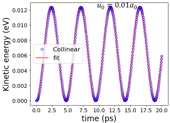
where $\bm{u}$ is the displacement vector, $\bm{u}_{0}$ is the displacement amplitude, $f_{ph}$ is the frequency of the phonon, $\bm{r}$ is the position and $t$ is the time. Here, periodic boundary conditions are used, and $k_{ph}=2\pi n/L$ , where $n$ is an integer and $L$ is the length of the simulated system along $\bm{k}_{ph}$ . Next, one runs spin-lattice dynamics (with initial velocities of atoms equal to zero to simulate sound velocity at zero-temperature) using the microcanonical ensemble NVE for at least few periods of the kinetic energy. In our simulation we set the time step $dt=1$ fs, and we verify that the total energy is preserved. Last, the phonon frequency $f_{ph}$ is extracted from the fitting of the kinetic energy ( $E_{K}$ ) versus timeKia et al. 2004

\displaystyle E_{K}(t)=A\left[1-\cos(4\pi f_{ph}t)\right].

(11)

where $A$ is a fitting parameter that does not depend on time since no attenuation of the sound wave takes place due to the lack of energy dissipation for these particular simulation conditions. Here, in the limit of low momentum ( $k_{ph}\xrightarrow{}0$ ), the phonon’s velocity (group velocity) $v_{ph}$ approaches the sound velocity $v$ in the solid (continuum theory) that can be expressed in terms of the elastic constants. For example, in the case of a sound wave propagating in the direction $[001]$ , one can approximately compute the sound velocity in the solid from the phonon’s frequency and momentum as

\displaystyle v\Bigg|_{\bm{u}}^{\bm{k}\parallel[001]}=\lim_{k_{ph}\rightarrow 0}v_{ph}\Bigg|_{\bm{u}}^{\bm{k}_{ph}\parallel[001]}=\frac{2\pi f_{ph}}{k_{ph}}\Bigg|_{\bm{u}}^{\bm{k}_{ph}\parallel[001]}.

(12)

In our calculations, we use a system size $10\times 10\times 120$ unit cells ( $24000$ atoms, $L=120a_{0}$ ) with lattice parameter $a_{0}^{c}$ and low phonon momentum $n=1$ ( $k_{ph}=2\pi/(120a_{0})$ ) for BCC Fe at collinear state, see Fig.1. In the case of paramagnetic-like state, we increase the system size up to $30\times 30\times 120$ unit cells ( $216000$ atoms) with lattice parameter $a_{0}^{r}$ , as discussed in Section IV.1. The simulations are performed using the SPIN packageTranchida et al. 2018 of LAMMPSThompson et al. 2022. As first benchmark of this method, we study the influence of the displacement amplitude $\bm{u}_{0}$ on the calculated frequency for a transverse phonon propagating in the direction $\bm{k}_{ph}\parallel[001]$ with polarization $\bm{u}\parallel[100]$ . The results are shown in Fig.2. We see that below $u_{0}=0.01a_{0}$ the frequency is not significantly affected by this parameter, so we use this value for our calculations. The fitting to extract the frequency for this case (collinear state without SOC) is shown in Fig.3. The calculated velocity using Eq.12 with the fitted frequency $f_{ph}^{c}$ and the value of $k_{ph}^{c}=2\pi/(120a_{0}^{c})$ is $v_{ph}^{c}=3602.2$ m/s. Note that in this method to further reduce the phonon’s momentum ( $k_{ph}\xrightarrow{}0$ ) one needs to increase the system size ( $L$ ) making the simulations more demanding computationally. On the other hand, one advantage of this method is that could be used to study the MEL effects on the attenuation of sound wavesKia et al. 2004; Simon 1958; Sakurai 1964; de Lacheisserie 1993 through the time dependence of the fitting parameter $A(t)$ in Eq.11 within a simulation that allows energy dissipation. The study of MEL effects on the attenuation of sound waves is not performed in the present work.

Refer to caption — Figure 1: Initial atomic displacement of a transverse phonon mode propagating in the direction $\bm{k}_{ph}\parallel[001]$ with polarization $\bm{u}\parallel[100]$ for BCC Fe. The system size is $10\times 10\times 120$ unit cells, while the displacement amplitude is $u_{0}=0.01a_{0}$ . The phonon momentum is $k_{ph}=2\pi/(120a_{0})$ .

II.3.2 Finite displacement method

To overcome the size limitations of the method based on the oscillation of the kinetic energy, one can use the FDMTogo and Tanaka 2015. In the FDM, the phonon’s frequency is derived from the forces associated with a systematic set of displacements. Here, we use this method, as implemented in the program PHONOPYTogo and Tanaka 2015; pho, also leveraging the PHONOLAMMPSCarreras interface between PHONOPY and LAMMPS. The group velocity of the phonon is computed aspho

\displaystyle v_{ph}(\bm{k},j)=\frac{1}{4\pi f_{ph}(\bm{k},j)}\Big\langle\bm{e}(\bm{k},j)\Big|\frac{\partial D(\bm{k})}{\partial\bm{k}}\Big|\bm{e}(\bm{k},j)\Big\rangle,

(13)

where $j$ is the phonon’s band index, $D$ is the dynamical matrix and $\bm{e}$ is the phonon polarization vector. For the collinear calculations we generate a supercell with size $4\times 4\times 4$ with lattice parameter $a_{0}^{c}$ , while for the paramagnetic states we use $16\times 16\times 16$ with lattice parameter $a_{0}^{r}$ . The atomic displacement distance is set to its default value $0.01$ Å. Since in this method we do not have size limitations for studying phonons with very low momentum ( $k_{ph}\xrightarrow{}0$ ), we compute the frequency and group velocity for a phonon with momentum $k_{ph}=2\pi/(12000a_{0})$ . For example, in the case of a transverse phonon at a collinear state propagating in the direction $\bm{k}_{ph}\parallel[001]$ with very low momentum $\bm{k}=(0,0,2\pi/(12000a_{0}^{c}))$ , the calculated group velocity with the FDM is $v_{ph}^{c}=3601.2$ m/s, which is quite close to the value obtained with the oscillation of the kinetic energy ( $v_{ph}^{c}=3602.2$ m/s).

II.3.3 Corrections to elastic constants

As third method, we consider the MEL effects as corrections to elastic constants. A detailed description of this approach is given in Appendix A. For example, in the case of a transverse sound wave propagating in the direction $\bm{k}_{ph}\parallel[001]$ with polarization $\bm{u}\parallel[100]$ at a collinear state without SOC, we have

\displaystyle v^{c}\Bigg|_{\bm{u}\parallel[100]}^{\bm{k}\parallel[001]}=\sqrt{\frac{C^{c}_{44}}{\rho^{c}}},

(14)

where $\rho^{c}$ is the density of the material at the collinear state. Using the elastic constant $C^{c}_{44}$ and density $\rho^{c}$ (see Table 2) at the collinear state in Eq.14, we find $v^{c}=3615.7$ m/s. Although slightly larger than the previously simulated phonon’s velocity with the oscillation of the kinetic energy and FDM, this remains within a close agreement.

III Theory of magnetoelastic effects on sound velocity

In this section we provide a brief overview of the main theoretical isotropic and anisotropic MEL effects on sound velocity. To facilitate the analysis of the simulations, it is convenient to decompose the isotropic and anisotropic MEL effects on the fractional change in velocity as follows

		$\displaystyle\frac{v^{SOC}-v^{r}}{v^{r}}=\frac{v^{c}-v^{r}}{v^{r}}+\frac{v^{SOC}-v^{c}}{v^{r}}$		(15)
		$\displaystyle=\frac{v^{c}-v^{r}}{v^{r}}+\frac{v^{SOC}-v^{c}}{v^{c}}\cdot\frac{1}{1-\left(\frac{v^{c}-v^{r}}{v^{c}}\right)}$
		$\displaystyle=\frac{v^{c}-v^{r}}{v^{r}}+\frac{v^{SOC}-v^{c}}{v^{c}}\cdot\left[1+\left(\frac{v^{c}-v^{r}}{v^{c}}\right)+...\right]$
		$\displaystyle\simeq\frac{v^{c}-v^{r}}{v^{r}}+\frac{v^{SOC}-v^{c}}{v^{c}}+O\left[\left(\frac{v^{SOC}-v^{r}}{v^{c}}\right)\cdot\left(\frac{v^{c}-v^{r}}{v^{c}}\right)\right],$

where $v^{SOC}$ is the sound velocity at a collinear state including isotropic exchange and SOC interactions, $v^{r}$ is the sound velocity assuming randomly oriented atomic magnetic moments (paramagnetic-like state) including only isotropic exchange interaction, and $v^{c}$ is the sound velocity at a collinear state including only isotropic exchange interaction. In the last step, we assumed that the change in the sound velocity due to MEL effects is small in comparison to the sound velocity ( $|v^{SOC}-v^{c}|/v^{c}\ll 1$ , $|v^{c}-v^{r}|/v^{r}\ll 1$ ), which is a reasonable approximation for the material studied here.

In experiment, the sound velocity is typically measured through the pulse echo methodTRUELL et al. 1969. The measured frequency with this technique $F$ is related to the sound velocity $v$ and sample length $l$ along the direction of the wave propagation through the following equationTRUELL et al. 1969; Thurston and Brugger 1964; Rouchy et al. 1981

\displaystyle v(F,l)=2Fl.

(16)

Performing a Taylor expansion of sound velocity yields

	$\displaystyle v(F,l)$	$\displaystyle=v(F_{0},l_{0})+\left(\frac{\partial v}{\partial F}\right)_{l=l_{0}}(F-F_{0})+\left(\frac{\partial v}{\partial l}\right)_{F=F_{0}}(l-l_{0})$		(17)
		$\displaystyle=v_{0}+2l_{0}(F-F_{0})+2F_{0}(l-l_{0}),$		(17)

where $v(F_{0},l_{0})=v_{0}=2F_{0}l_{0}$ . If we subtract $v_{0}$ from both sides of Eq.17 and divide both sides by $v_{0}$ , then we obtainRouchy and du Tremolet de Lacheisserie 1979; de Lacheisserie 1993

\displaystyle\frac{v-v_{0}}{v_{0}}=\frac{F-F_{0}}{F_{0}}+\frac{l-l_{0}}{l_{0}}.

(18)

The theoretical expressions for the fractional change in pulse echo frequency $F$ have been derived by Rouchy et al.Rouchy and du Tremolet de Lacheisserie 1979; Rouchy et al. 1980; de Lacheisserie 1993. In addition to this contribution, in Eq.18 we see that the fractional change in length along the direction of wave propagation must be also calculated in order to compute the fractional change in velocity. This fractional change in length arises from the magnetostriction induced by MEL interactions, and its general form for an arbitrary measuring length direction $\bm{\beta}$ is given by Eq.63.

The first term in the right-hand side of Eq.15 corresponds to the fractional change in sound velocity due to the isotropic exchange interaction (isotropic MEL effects)de Lacheisserie 1993; Rouchy and du Tremolet de Lacheisserie 1979

	$\displaystyle\frac{v^{c}-v^{r}}{v^{r}}\Bigg\|_{\bm{u}}^{\bm{k}}$	$\displaystyle=\frac{F^{c}-F^{r}}{F^{r}}\Bigg\|_{\bm{u}}^{\bm{k}}+\frac{l^{c}-l^{r}}{l^{r}}\Bigg\|^{\bm{k}},$		(19)
	$\displaystyle\frac{F^{c}-F^{r}}{F^{r}}\Bigg\|_{\bm{u}}^{\bm{k}}$	$\displaystyle=Y(m^{\alpha,2}_{i})\Bigg\|_{\bm{u}}^{\bm{k}},$		(19)

where $Y(m^{\alpha,2}_{i})$ is a function that depends on the isotropic morphic coefficients $m^{\alpha,2}_{i}$ . The form of this function also depends on the propagation direction of the wave $\bm{k}$ and polarization $\bm{u}$ but not on the magnetization direction $\bm{M}$ , since this MEL effect is isotropic. In this isotropic case, the fractional change in length depends only on the propagation direction of the wave. The second term in the right hand side of Eq.15 gives the anisotropic MEL effects due to the SOC, and may be splitted into the following termsde Lacheisserie 1993; Rouchy and du Tremolet de Lacheisserie 1979; Rouchy et al. 1980

$\displaystyle\frac{v^{SOC}-v^{c}}{v^{c}}\Bigg\|_{\bm{u}}^{\bm{k},\bm{M}}$	$\displaystyle=\frac{F^{SOC}-F^{c}}{F^{c}}\Bigg\|_{\bm{u}}^{\bm{k},\bm{M}}+\frac{l^{SOC}-l^{c}}{l^{c}}\Bigg\|^{\bm{k},\bm{M}},$	(20)
$\displaystyle\frac{F^{SOC}-F^{c}}{F^{c}}\Bigg\|_{\bm{u}}^{\bm{k},\bm{M}}$	$\displaystyle=G(m^{\gamma,2}_{i},m^{\epsilon,2}_{i})\Bigg\|_{\bm{u}}^{\bm{k},\bm{M}}+R(\lambda^{\gamma,2},\lambda^{\epsilon,2})\Bigg\|_{\bm{u}}^{\bm{k},\bm{M}}$
	$\displaystyle+S(H)\Bigg\|_{\bm{u}}^{\bm{k},\bm{M}},$

where $G(m^{\gamma,2}_{i},m^{\epsilon,2}_{i})$ is a function that depends on anisotropic morphic coefficients $m^{\gamma,2}_{i}$ and $m^{\epsilon,2}_{i}$ which are linear combinations of second order in strain MEL constants and third order in strain elastic constants, $R(\lambda^{\gamma,2},\lambda^{\epsilon,2})$ is a function that comes from rotational and magnetostrictive effectsRouchy et al. 1980 and depends on anisotropic magnetostrictive coefficients $\lambda^{\gamma,2}$ and $\lambda^{\epsilon,2}$ , and $S(H)$ is a field-dependent term derived by Simon Simon 1958. The form of these functions also depends on $\bm{k}$ , $\bm{u}$ and $\bm{M}$ . The fractional change in length depends on $\bm{k}$ and $\bm{M}$ but not on the polarization $\bm{u}$ . The relationship between the morphic coefficients and higher order elastic and MEL constants are given in Eq.65, where we use the same definitions as in Ref.Rouchy et al. 1980. Eqs.19 and 20 are derived from the free energy by solving the coupled elastic and magnetic equations of motion Simon 1958; Rouchy and du Tremolet de Lacheisserie 1979; Rouchy et al. 1980; Ikeda 1982; de Lacheisserie 1993. A theoretical description of all these effects can also be provided by expanding the internal energy as a series of the Lagrangian tensor components, as well as symmetrical and antisymmetrical components of the homogeneous strains Rouchy and du Tremolet de Lacheisserie 1979. The explicit form of these equations for the simulated cases is shown in Section IV. Alternatively, one can also take into account MEL effects on sound velocity as corrections to the elastic constants Rinaldi and Turilli 1985; de Lacheisserie 1993. We describe this approach in Appendix A.

IV Results

IV.1 Isotropic magnetoelastic effects

In the case of a transverse wave propagating along $\bm{k}\parallel[001]$ with polarization $\bm{u}\parallel[100]$ , Eq.19 readsRouchy and du Tremolet de Lacheisserie 1979

$\displaystyle\frac{v^{c}-v^{r}}{v^{r}}\Bigg\|_{\bm{u}\parallel[100]}^{\bm{k}\parallel[001]}$	$\displaystyle=\frac{F^{c}-F^{r}}{F^{r}}\Bigg\|_{\bm{u}\parallel[100]}^{\bm{k}\parallel[001]}+\frac{l^{c}-l^{r}}{l^{r}}\Bigg\|^{\bm{k}\parallel[001]},$	(21)
$\displaystyle\frac{F^{c}-F^{r}}{F^{r}}\Bigg\|_{\bm{u}\parallel[100]}^{\bm{k}\parallel[001]}$	$\displaystyle=Y(m_{i}^{\alpha,2})\Bigg\|_{\bm{u}\parallel[100]}^{\bm{k}\parallel[001]}=\frac{m_{3}^{\alpha,2}}{12C^{c}_{44}},$
$\displaystyle\frac{l^{c}-l^{r}}{l^{r}}\Bigg\|^{\bm{k}\parallel[001]}$	$\displaystyle=\frac{a_{0}^{c}-a_{0}^{r}}{a_{0}^{r}},$

where $m_{3}^{\alpha,2}$ is an isotropic morphic coefficient defined in Eq.65. The form of function $Y$ is the same as in Ref.Rouchy and du Tremolet de Lacheisserie 1979, but note that it is not the same as in Ref.de Lacheisserie 1993 due to a different definition of morphic coeffcients and high order MEL constants. The fractional change in length along $[001]$ arises from volume magnetostriction $\omega_{s}$ due to the exchange interaction. Here, to calculate $v^{r}$ we consider two types of paramagnetic-like state: (i) with randomly oriented magnetic moments along 3D directions, and (ii) random up-down orientationsAlling et al. 2010. To simulate the purely isotropic MEL effects, we do not include SOC interaction (dipole and quadrupole Néel’s terms) in the spin-lattice model. In Fig.4 we show the calculated EOS of BCC Fe at these paramagnetic-like states using system sizes $10\times 10\times 120$ and $30\times 30\times 120$ unit cells. We observe that increasing the system size up to $30\times 30\times 120$ gives similar EOS for both types of paramagnetic-like states, so that we use this size to calculate $v^{r}$ through the method based on the oscillation of the kinetic energy. Moreover, since this system size is sufficiently large, we do not need to compute $v^{r}$ for several random configurations and average them, or use special quasi-random structure (SQS) methodAlling et al. 2010. Note that for the collinear state we do not need such a large size, so that we use a system size $10\times 10\times 120$ unit cells to compute $v^{c}$ . In Fig.5 we show the calculated kinetic energy versus time for BCC Fe at these two considered paramagnetic-like states. Here, we simulated three cases using an initial displacement amplitude $u_{0}=0.01a_{0}$ , $u_{0}=0.05a_{0}$ and $u_{0}=0.1a_{0}$ . We see that the paramagnetic-like state with randomly oriented magnetic moments along 3D directions increases the kinetic energy rapidly, so that it is not possible to fit this behaviour to Eq. 11. This is due to the fact that this spin configuration corresponds to a thermal equilibrium state with spin temperature $T_{spin}$ above $T_{C}=1043K$ ( $T_{spin}>T_{C}$ ), hence the spin system interchanges energy with the phonon system, which is initially at zero-temperature ( $T_{ph}=0$ K), trying to equilibrate their temperaturesTranchida et al. 2018. Consequently, the lattice temperature increases rapidly, as seen in the dynamics of the kinetic energy. On the other hand, the configuration with random up-down spins is a paramagnetic-like state in terms of the total energy but it does not correspond to a thermally equilibrated state above $T_{C}$ . For example, the spin temperature for this state using the definition of Nurdin et al.Nurdin and Schotte 2000; Tranchida et al. 2018 is $T_{spin}=0$ K. Hence, it can mechanically stabilize the oscillation of the kinetic energy by introducing a small energy shift ( $\sim 65$ eV $=0.3$ meV/atom) on the kinetic energy (Eq.11). In this case, we can extract the frequency of the sound wave $f^{r}$ (do not confuse with the measured frequency $F$ in the pulse echo method) if the initial displacement amplitude $u_{0}$ is sufficiently large ( $u_{0}>0.01a_{0}$ ) to overcome the noise fluctuations of the kinetic energy. From the fitting we obtain the frequency $f^{r}=0.111619$ THz. We can estimate the sound velocity at the paramagnetic state by inserting the calculated $f^{r}$ and $k^{r}=2\pi/(120a_{0}^{r})$ in Eq.12, finding $v^{r}=3776.4$ m/s. At the collinear state, we obtain the frequency $f^{c}=0.106063$ THz. Hence, the estimated sound velocity using Eq.12 is $v^{c}=3602.2$ m/s. Consequently, using Eq.12 leads to a fractional change in velocity $(v^{c}-v^{r})/v^{r}=-0.0435$ .

The FDM is a more rigorous and accurate approach to compute $v^{r}$ than the oscillation of the kinetic energy since it has no problems associated with the spin-phonon stability for the paramagnetic-like states at zero-temperature. Applying the methodology described in Section II.3.2, the FDM gives $(v^{c}-v^{r})/v^{r}=-0.048$ and $-0.0408$ for paramagnetic-like state with randomly oriented magnetic moments in 3D and randomly up-down orientations, respectively. Alternatively, we can also estimate it by using the corrections to elastic constants, as explained in Section II.3.3 and Appendix A. For example, using the elastic constant $C^{r}_{44}$ and density $\rho^{r}$ at the paramagnetic state (see Table 2) in Eq.14 gives $v^{r}=3807.9$ m/s, while for the collinear state we get $v^{c}=3615.7$ m/s. This gives $(v^{c}-v^{r})/v^{r}=-0.0505$ . Therefore, we see that the fractional change in velocity obtained with the three approaches (from the oscillation of the kinetic energy, FDM and corrections to elastic constants) are consistent with each other. Last, we can also estimate the isotropic morphic coefficient $m_{3}^{\alpha,2}$ by inserting the calculated sound velocities ( $v^{r}$ and $v^{c}$ ), equilibrium lattice parameters ( $a^{r}_{0}$ and $a^{c}_{0}$ ) and elastic constant $C^{c}_{44}$ in Eq.21. This procedure gives $m_{3}^{\alpha,2}=-60.8$ GPa using the velocities derived from the oscillation of the kinetic energy, and $m_{3}^{\alpha,2}=-66.5$ GPa and $-57.4$ GPa with the FDM for paramagnetic-like state with randomly oriented magnetic moments in 3D and randomly up-down orientations, respectively, while using the velocities given by the corrections to the elastic constants we find $m_{3}^{\alpha,2}=-69.7$ GPa.

In the case of a longitudinal wave propagating along $\bm{k}\parallel[001]$ with polarization $\bm{u}\parallel[001]$ , Eq.19 readsRouchy and du Tremolet de Lacheisserie 1979

$\displaystyle\frac{v^{c}-v^{r}}{v^{r}}\Bigg\|_{\bm{u}\parallel[001]}^{\bm{k}\parallel[001]}$	$\displaystyle=\frac{F^{c}-F^{r}}{F^{r}}\Bigg\|_{\bm{u}\parallel[001]}^{\bm{k}\parallel[001]}+\frac{l^{c}-l^{r}}{l^{r}}\Bigg\|^{\bm{k}\parallel[001]},$	(22)
$\displaystyle\frac{F^{c}-F^{r}}{F^{r}}\Bigg\|_{\bm{u}\parallel[001]}^{\bm{k}\parallel[001]}$	$\displaystyle=Y(m_{i}^{\alpha,2})\Bigg\|_{\bm{u}\parallel[001]}^{\bm{k}\parallel[001]}=\frac{m_{1}^{\alpha,2}}{3C^{c}_{11}},$
$\displaystyle\frac{l^{c}-l^{r}}{l^{r}}\Bigg\|^{\bm{k}\parallel[001]}$	$\displaystyle=\frac{a_{0}^{c}-a_{0}^{r}}{a_{0}^{r}},$

where $m_{1}^{\alpha,2}$ is an isotropic morphic coefficient defined in Eq.65. Following the same procedure as before and using Eq.22, we find $m_{1}^{\alpha,2}=-10.6$ GPa and $-8.0$ GPa through the FDM for paramagnetic-like state with randomly oriented magnetic moments in 3D and randomly up-down orientations, respectively, and $m_{1}^{\alpha,2}=-4.6$ GPa via the corrections to the elastic constants. Unfortunately, for the simulated cases of the longitudinal mode, the oscillation of the kinetic energy was not sufficiently stable to extract the frequency at the paramagnetic-like state ( $f^{r}$ ), so that we could not estimate $m_{1}^{\alpha,2}$ with this approach. In Table 3, we present a summary of the results obtained for the two isotropic morphic coefficients of BCC Fe calculated in this work. We point out that the elastic constants at the paramagnetic state ( $C^{r}_{ij}$ ) and the isotropic morphic coefficients ( $m^{\alpha}$ ) are sensitive to the volume magnetostriction $\omega_{S}$ of the spin-lattice model.

Table 3: Calculated isotropic morphic coefficients of a wave propagating along

\bm{k}\parallel[001]

using the spin-lattice model of BCC Fe without SOC.

Method

\bm{u}

Paramagnetic

State

Morphic

coefficient

GPa

Kinetic energy

\bm{u}\parallel[100]

Random in 3D

m_{3}^{\alpha,2}

Random up-down

-60.8

FDM

Random in 3D

-66.5

Random up-down

-57.4

Elastic constants

Random in 3D

-69.7

Kinetic energy

\bm{u}\parallel[001]

Random in 3D

m_{1}^{\alpha,2}

Random up-down

FDM

Random in 3D

-10.6

Random up-down

-8.0

Elastic constants

Random in 3D

-4.6

IV.2 Anisotropic magnetoelastic effects

For the analysis of anisotropic effects we follow the same procedure, but now we switch on the SOC (dipole and quadrupole Néel’s terms) in order to compute the velocity $v^{SOC}$ . We first consider a transverse wave propagating along $\bm{k}\parallel[001]$ with polarization $\bm{u}\parallel[100]$ and magnetization $\bm{M}\bot[001]$ . In this case, the functions in Eq. 20 readRouchy et al. 1980

		$\displaystyle G\Bigg\|_{\bm{u}\parallel[100]}^{\bm{k}\parallel[001]\bot\bm{M}}=\frac{m_{3}^{\gamma,2}}{8C^{c}_{44}}\left(\frac{1}{3}-\cos 2\phi\right),$		(23)
		$\displaystyle R\Bigg\|_{\bm{u}\parallel[100]}^{\bm{k}\parallel[001]\bot\bm{M}}=\frac{1}{2}(\lambda^{\gamma,2}-\lambda^{\epsilon,2})\left[1+\cos 2\phi\right]$
		$\displaystyle=\frac{3}{4}(\lambda_{001}-\lambda_{111})\left[1+\cos 2\phi\right],$
		$\displaystyle S\Bigg\|_{\bm{u}\parallel[100]}^{\bm{k}\parallel[001]\bot\bm{M}}=-\frac{(B^{\epsilon,2})^{2}(1+\cos 2\phi)}{4C^{c}_{44}\mu_{0}M_{s}\left(H+M_{s}+H_{D}+\frac{K_{1}[3+\cos 4\phi]}{2\mu_{0}M_{s}}\right)},$
		$\displaystyle H\gg\frac{2K_{1}}{\mu_{0}M_{s}},$
		$\displaystyle\frac{l^{SOC}-l^{c}}{l^{c}}\Bigg\|^{\bm{k}\parallel[001]\bot\bm{M}}=-\frac{1}{3}\lambda^{\gamma,2}=-\frac{1}{2}\lambda_{001},$

where $\phi$ is the angle between $\bm{M}$ and crystallographic direction $[100]$ and $H_{D}$ is the demagnetizing field. In our simulations $H_{D}=0$ since we do not include dipole-dipole interactions. The MEL constant $B^{\epsilon,2}=b_{2}$ and magnetostrictive coefficients $\lambda^{\gamma,2}=3\lambda_{001}/2$ and $\lambda^{\epsilon,2}=3\lambda_{111}/2$ are defined in Appendix B. The form of function $G$ is the same as in Ref.Rouchy and du Tremolet de Lacheisserie 1979, but note that it is not the same as in Ref.de Lacheisserie 1993 due to a different definition of morphic coeffcients and high order MEL constants. The fractional change in length along $[001]$ is obtained from the anisotropic part of Eq.63. The fractional change in velocity obtained from the oscillation of the kinetic energy and the FDM for the spin-lattice model of BCC Fe is shown in Fig.6. It is performed at high applied magnetic field $\mu_{0}H=40$ T where $\bm{H}\parallel\bm{M}$ . In analogy to experiment, we extract the morphic coeffcient $m_{3}^{\gamma,2}$ by fitting the results given by the spin-lattice simulations to the summation of functions $G$ , $R$ , $S$ and $(l^{SOC}-l^{c})/l^{c}$ in Eq.23. Here, all materials parameters in these functions are constrained to corresponding values of the spin-lattice model (see Table 2), except $m_{3}^{\gamma,2}$ which is a fitting parameter. This procedure gives $m_{3}^{\gamma,2}=-14.3$ MPa for method based on the oscillation of the kinetic energy, and $m_{3}^{\gamma,2}=-15.3$ MPa using the FDM. In Fig.6 we also calculated the fractional change in velocity using the corrections to the elastic constants given by Eq.49. We see that this approach gives similar results to the field-dependent function $S(H)$ , since the linear MEL theory (which does not include high order MEL terms) was used both by SimonSimon 1958 to derive function $S(H)$ and Rinaldi et al.Rinaldi and Turilli 1985 to obtain the SOC corrections ( $\triangle C^{SOC}$ ) to the elastic constantsde Lacheisserie 1993.

The case of a transverse wave propagating along $\bm{k}\parallel[001]$ with polarization $\bm{u}\parallel[100]$ and magnetization $\bm{M}\parallel[100]$ is a particular case of Eq.24 when $\phi=0$ . This case is calculated using the spin-lattice model for different values of the applied field in Fig.7. Here, we also plot the case when the magnetization is $\bm{M}\parallel[001]$ , where the functions in Eq. 20 now readRouchy et al. 1980

		$\displaystyle G\Bigg\|_{\bm{u}\parallel[100]}^{\bm{k}\parallel\bm{M}\parallel[001]}=-\frac{m_{3}^{\gamma,2}}{12C^{c}_{44}},$		(24)
		$\displaystyle R\Bigg\|_{\bm{u}\parallel[100]}^{\bm{k}\parallel\bm{M}\parallel[001]}=\lambda^{\epsilon,2}-\lambda^{\gamma,2}=\frac{3}{2}(\lambda_{111}-\lambda_{001}),$
		$\displaystyle S\Bigg\|_{\bm{u}\parallel[100]}^{\bm{k}\parallel\bm{M}\parallel[001]}=-\frac{(B^{\epsilon,2})^{2}}{2C^{c}_{44}\mu_{0}M_{s}\left(H+H_{D}+\frac{2K_{1}}{\mu_{0}M_{s}}\right)},\quad H\gg\frac{2K_{1}}{\mu_{0}M_{s}},$
		$\displaystyle\frac{l^{SOC}-l^{c}}{l^{c}}\Bigg\|^{\bm{k}\parallel\bm{M}\parallel[001]}=\frac{2}{3}\lambda^{\gamma,2}=\lambda_{001},$

In Fig. 7, we see that both calculated cases ( $\bm{M}\parallel[100]$ and $\bm{M}\parallel[001]$ ) are in good agreement with the theory at high applied magnetic fields ( $\mu_{0}H>5$ T). In this figure, we used the previously calculated value $m_{3}^{\gamma,2}=-14.3$ MPa derived from the oscillation of the kinetic energy in order to plot the theoretical function $G$ , while for the other parameters in Eqs.23 and 24 we set the values of the spin-lattice model (see Table 2). We also see that the spin-lattice model can correctly reproduce the rotational-magnetostrictive effect at high applied magnetic fields predicted by Eqs.23 and 24, that is

		$\displaystyle\lim_{H\to\infty}\left[\frac{v^{SOC}-v^{c}}{v^{c}}\Bigg\|_{\bm{u}\parallel\bm{M}\parallel[100]}^{\bm{k}\parallel[001]}-\frac{v^{SOC}-v^{c}}{v^{c}}\Bigg\|_{\bm{u}\parallel[100]}^{\bm{k}\parallel\bm{M}\parallel[001]}\right]$		(25)
		$\displaystyle=\left[R\Bigg\|_{\bm{u}\parallel\bm{M}\parallel[100]}^{\bm{k}\parallel[001]}+\frac{l^{SOC}-l^{c}}{l^{c}}\Bigg\|^{\bm{k}\parallel[001]}_{\bm{M}\parallel[100]}\right]$
		$\displaystyle-\left[R\Bigg\|_{\bm{u}\parallel[100]}^{\bm{k}\parallel\bm{M}\parallel[001]}+\frac{l^{SOC}-l^{c}}{l^{c}}\Bigg\|^{\bm{k}\parallel\bm{M}\parallel[001]}\right]$
		$\displaystyle=2(\lambda^{\gamma,2}-\lambda^{\epsilon,2})-\frac{3}{2}\lambda_{001}=\frac{3}{2}\lambda_{001}-3\lambda_{111}.$

The factor $2(\lambda^{\gamma,2}-\lambda^{\epsilon,2})$ arises from the rotational-magnetostrictive effect in the fractional change in pulse echo frequency $F$ , as shown in Refs.Rouchy and du Tremolet de Lacheisserie 1979; Rouchy et al. 1980; de Lacheisserie 1993, while the additional factor $-3\lambda_{001}/2$ comes from the fractional change in length. The fractional change in velocity derived from the corrections to elastic constants (Eq. 49) approaches the field-dependent function $S(H)$ at high fields along $\bm{H}\parallel[001]$ , but it does not reproduce the high order effects since the used corrections to the elastic constants are based on the linear MEL theoryRinaldi and Turilli 1985. The results from the spin-lattice simulations exhibit a non-monotonic behaviour at low applied magnetic fields ( $\mu_{0}H<5$ T). Similar pattern has been experimentally observed in single cubic crystals of disordered Co-Pt alloyRouchy et al. 1980. Note that the low-field regime can not be described by the current theory since the field-dependent term $S(H)$ was derived by Simon only under the assumption of high applied magnetic fieldsSimon 1958 ( $H\gg 2K_{1}/[\mu_{0}M_{s}]$ ). Hence, we see that the spin-lattice simulations could be a useful tool to explore and understand the physics of MEL effects on sound velocity in this regime.

Let us now consider a longitudinal wave propagating along $\bm{k}\parallel[001]$ with polarization $\bm{u}\parallel[001]$ . If the magnetization is along $\bm{M}\parallel[001]$ , then functions in Eq. 20 readRouchy et al. 1980

		$\displaystyle G\Bigg\|_{\bm{u}\parallel[001]}^{\bm{k}\parallel[001]\parallel\bm{M}}=\frac{2m_{1}^{\gamma,2}}{3C^{c}_{11}},$		(26)
		$\displaystyle R\Bigg\|_{\bm{u}\parallel[001]}^{\bm{k}\parallel[001]\parallel\bm{M}}=0,$
		$\displaystyle S\Bigg\|_{\bm{u}\parallel[001]}^{\bm{k}\parallel[001]\parallel\bm{M}}=0,$
		$\displaystyle\frac{l^{SOC}-l^{c}}{l^{c}}\Bigg\|^{\bm{k}\parallel[001]\parallel\bm{M}}=\frac{2}{3}\lambda^{\gamma,2}=\lambda_{001},$

while if the magnetization is along $\bm{M}\parallel[100]$ , then we haveRouchy et al. 1980

\displaystyle\frac{v^{SOC}-v^{c}}{v^{c}}\Bigg|_{\bm{u}\parallel[001]}^{\bm{k}\parallel[001],\bm{M}\parallel[100]}=-\frac{1}{2}\frac{v^{SOC}-v^{c}}{v^{c}}\Bigg|_{\bm{u}\parallel[001]}^{\bm{k}\parallel\bm{M}\parallel[001]}.

(27)

We simulated these two cases for different values of the applied magnetic field in Fig.8. The spin-lattice simulations give a constant fractional change in velocity as a function of the applied field, which is consistent with the lack of field dependency ( $S(H)=0$ ) in Eqs. 26 and 27. We also see that it correctly reproduces the relationship provided by Eq. 27, which comes from a high order effect induced by the anisotropic morphic coefficient $m_{1}^{\gamma,2}$ via the function $G$ and fractional change in length. We can derive the morphic coefficient $m_{1}^{\gamma,2}$ by fitting the summation of the functions in Eq. 26, where the values for $C^{c}_{11}$ and $\lambda_{001}$ are taken from Table 2, to the fractional change in velocity given by the spin-lattice simulations in Fig.8. This procedure gives $m_{1}^{\gamma,2}=2.4$ MPa using both the FDM and the oscillation of the kinetic energy. The fractional change in velocity derived from the corrections to elastic constants (Eq. 51) is zero for both cases ( $\bm{M}\parallel[001]$ and $\bm{M}\parallel[100]$ ) because $\triangle S^{SOC}_{33}(H)=0$ , as expected from the fact that $S(H)=0$ in Eq.26.

Table 4: Calculated anisotropic morphic coefficients of the spin-lattice model for BCC Fe.

Method

Morphic

coefficient

MPa

Kinetic energy

m_{3}^{\gamma,2}

-14.3

FDM

-15.3

Kinetic energy

m_{1}^{\gamma,2}

2.4

FDM

2.4

In Table 4, we present a summary of the two anisotropic morphic coefficients derived for the spin-lattice model of BCC Fe in this work. There are in total 9 morphic coefficients $m^{\mu,2}_{i}$ (where $\mu=\alpha,\beta,\gamma$ and $i=1,2,3$ ) up to second order in the direction cosine of magnetization, see Appendix BRouchy and du Tremolet de Lacheisserie 1979; Rouchy et al. 1980; de Lacheisserie 1993. Although some of these morphic coefficients were not computed in this study, they can be evaluated in a similar way by choosing other propagating directions of the waveRouchy et al. 1980. In Tables 3 and 4 we see that the isotropic morphic coefficient $m_{3}^{\alpha,2}$ (induced by the exchange interaction) is about four orders of magnitude larger than the anisotropic ones. This result is in good agreement with morphic coefficients reported for FCC Ni, where similar differences were observed de Lacheisserie 1993; du Tremolet de Lacheisserie and Rouchy 1982. Note that the extrapolation of the calculated morphic coefficients with this spin-lattice model to experiment is not obvious because they are linear combinations of third order in strain elastic constants ( $\tilde{C}_{ijk}$ ) and second order in strain MEL constants ( $\tilde{M}^{\mu,2}_{i}$ ) Rouchy and du Tremolet de Lacheisserie 1979; Rouchy et al. 1980; de Lacheisserie 1993. The SNAP interatomic potential used in the model might describe, at least to some extent, experimental high order elastic constants thanks to its quantum mechanical derivation and complex functional form Nikolov et al. 2021; Thompson et al. 2015. However, it is not clear that the Néel model used in this work could be sufficiently accurate to describe correctly experimental high order MEL constants $\tilde{M}^{\mu,2}_{i}$ since it was originally designed to reproduce the experimental MEL constants $B^{\mu,2}$ only up to first order in strainNieves et al. 2021a. Possible deviations due to the Néel model might not be relevant in the calculation of those morphic coefficients where the contribution of high order elastic constants is much greater than the high order MEL constants ( $\tilde{M}^{\mu,2}_{i}\ll\tilde{C}_{ljk}\lambda^{\mu,2}$ , see Eq.65)Rouchy et al. 1980.

IV.3 Magnetoelastic effects on phonon dispersion

In previous sections, we studied the MEL effects on phonons with low momentum ( $k_{ph}\rightarrow 0$ ) in order to compare the atomistic simulations with the continuum theory of sound velocity in a solid. Here, we extend our study by calculating the MEL effects on the frequency of phonons with larger momentum. In particular, we compute the phonon dispersion along the $\Gamma-$ H line of k-points, see Fig.9. In general, we observe small changes in phonon’s frequency due to MEL effects. For comparison, we also plot in Fig.9 the Density-Functional Theory (DFT) calculations performed by Ikeda et al.Ikeda et al. 2014 using SQS with size $2\times 2\times 2$ . Close to the $\Gamma$ point ( $k_{ph}\rightarrow 0$ ), our calculations with the spin-lattice model are very similar to the DFT results reported in Ref.Ikeda et al. 2014. However, at higher values of $k$ , we obtain that the phonon frequencies of the paramagnetic state are slightly larger than in the ferromagnetic state, while the opposite behaviour was found by Ikeda et al.Ikeda et al. 2014 with also a higher shift in the frequencies. Similar results as in Ref.Ikeda et al. 2014 have been reported by Novikov et al.Novikov et al. 2021 using DFT and magnetic moment tensor potentials. Finally, in Fig.10 we analyze how the fractional change in phonon group velocity is influenced by the magnitude of phonon momentum $k_{ph}$ . We observe a significant modification of $(v^{c}-v^{r})/v^{r}$ as we increase $k_{ph}$ , where the sign is changed in the middle of $\Gamma$ -H line. This result suggests that the theoretical equation derived for sound waves Eq.21 might only hold for phonon with low momentum ( $k_{ph}\rightarrow 0$ ). On the other hand, $(v^{SOC}-v^{c})/v^{c}$ is not so strongly affected by the magnitude of phonon momentum, which means that in some cases the theoretical fractional change in velocity derived for sound waves might still provide at least a reasonable qualitative description for phonons with larger momentum.

V Conclusions

In summary, through the analysis of the kinetic energy and forces, we found that the spin-lattice model for BCC Fe is capable to describe the four main MEL effects on sound velocity (isotropic exchange effects, anisotropic morphic effects, field dependent effects and rotational-magnetostrictive effects). We also showed that the alternative approach based on corrections to the elastic constants can correctly account for isotropic exchange effects and anisotropic field dependent effects, but not for high order anisotropic effects (like anisotropic morphic effects and rotational-magnetostrictive effects) because the used SOC corrections were derived from the linear MEL theoryRinaldi and Turilli 1985. In analogy to experiment, some morphic coefficients of this spin-lattice model were extracted from the analysis of the fractional change in frequency, exhibiting a similar order of magnitude as in FCC Nidu Tremolet de Lacheisserie and Rouchy 1982; de Lacheisserie 1993. In the low magnetic field regime, our simulations reveal an interesting non-monotonic dependence on the applied field of the fractional change in sound velocity, which cannot be described by the current theory since it is valid only at high applied fieldsSimon 1958. Hence, the presented computational framework could be a useful tool to explore and understand the field regimes still uncovered by the theory. Similarly, this approach could also be helpful to study the combination of magnetic and atomistic scale effects (like vacancies, impurities or complex defects) on sound velocity, as well as design novel technological magneto-acoustic applications.

Acknowledgement

This work was supported by the ERDF in the IT4Innovations national supercomputing center - path to exascale project (CZ.02.1.01/0.0/0.0/16-013/0001791) within the OPRDE and projects “e-INFRA CZ (ID:90140)” and Donau No. 8X20050 by The Ministry of Education, Youth and Sports of the Czech Republic. In addition, P.N. and D.L. acknowledge support from the H2020-FETOPEN no. 863155 s-NEBULA project. S. Nikolov is an employee of Sandia National Laboratories, a multimission laboratory managed and operated by National Technology and Engineering Solutions of Sandia, LLC, a wholly owned subsidiary of Honeywell International Inc., for the U.S. Department of Energy’s National Nuclear Security Administration under Contract DE-NA0003525. This paper describes objective technical results and analysis. Any subjective views or opinions that might be expressed in the paper do not necessarily represent the views of the U.S. Department of Energy or the United States Government.

Appendix A Magnetoelastic effects on sound velocity as corrections to the elastic constants

MEL effects on sound velocity can be described in terms of effective elastic constants. In this appendix, we present a brief review of this approach. Let us start by deriving the general expression of sound velocity in terms of the elastic constants. The equation of motion of an elastic wave is given byLandau and Lifshitz 1959

\displaystyle\rho\frac{\partial^{2}u_{i}}{\partial t^{2}}=\sum_{j=x,y,z}\frac{\partial\sigma_{ij}}{\partial r_{j}},\quad\quad i=x,y,z

(28)

where $\rho$ is the mass density, $\bm{u}$ is the displacement vector and $\sigma_{ij}$ is the stress tensor that is related to the fourth-order elastic stiffness tensor $c_{ijkl}$ and the second-order strain tensor $\epsilon_{ij}$ through the generalized Hooke’s law

\sigma_{ij}=\sum_{k,l=x,y,z}c_{ijkl}\epsilon_{kl},\quad i,j=x,y,z.

(29)

Using the symmetry of the stress and strain tensors, the Hooke’s law can be written in matrix notation as

\displaystyle\begin{pmatrix}\sigma_{xx}\\ \sigma_{yy}\\ \sigma_{zz}\\ \sigma_{yz}\\ \sigma_{zx}\\ \sigma_{xy}\\ \end{pmatrix}

\displaystyle=\begin{pmatrix}c_{xxxx}&c_{xxyy}&c_{xxzz}&c_{xxyz}&c_{xxzx}&c_{xxxy}\\ c_{yyxx}&c_{yyyy}&c_{yyzz}&c_{yyyz}&c_{yyzx}&c_{yyxy}\\ c_{zzxx}&c_{zzyy}&c_{zzzz}&c_{zzyz}&c_{zzzx}&c_{zzxy}\\ c_{yzxx}&c_{yzyy}&c_{yzzz}&c_{yzyz}&c_{yzzx}&c_{yzxy}\\ c_{zxxx}&c_{zxyy}&c_{zxzz}&c_{zxyz}&c_{zxzx}&c_{zxxy}\\ c_{xyxx}&c_{xyyy}&c_{xyzz}&c_{xyyz}&c_{xyzx}&c_{xyxy}\\ \end{pmatrix}\begin{pmatrix}\epsilon_{xx}\\ \epsilon_{yy}\\ \epsilon_{zz}\\ 2\epsilon_{yz}\\ 2\epsilon_{zx}\\ 2\epsilon_{xy}\\ \end{pmatrix}

(30)

To facilitate the manipulation of this equation it is convenient to define the following six-dimensional vectors (Voigt notation)

\displaystyle\bm{\tilde{\sigma}}=\begin{pmatrix}\tilde{\sigma}_{1}\\ \tilde{\sigma}_{2}\\ \tilde{\sigma}_{3}\\ \tilde{\sigma}_{4}\\ \tilde{\sigma}_{5}\\ \tilde{\sigma}_{6}\\ \end{pmatrix}=\begin{pmatrix}\sigma_{xx}\\ \sigma_{yy}\\ \sigma_{zz}\\ \sigma_{yz}\\ \sigma_{zx}\\ \sigma_{xy}\\ \end{pmatrix},\quad\quad\bm{\tilde{\epsilon}}=\begin{pmatrix}\tilde{\epsilon}_{1}\\ \tilde{\epsilon}_{2}\\ \tilde{\epsilon}_{3}\\ \tilde{\epsilon}_{4}\\ \tilde{\epsilon}_{5}\\ \tilde{\epsilon}_{6}\\ \end{pmatrix}=\begin{pmatrix}\epsilon_{xx}\\ \epsilon_{yy}\\ \epsilon_{zz}\\ 2\epsilon_{yz}\\ 2\epsilon_{zx}\\ 2\epsilon_{xy}\\ \end{pmatrix},

(31)

and replace $c_{ijkl}$ by $C_{nm}$ contracting a pair of cartesian indices into a single integer: $xx\rightarrow 1$ , $yy\rightarrow 2$ , $zz\rightarrow 3$ , $yz\rightarrow 4$ , $zx\rightarrow 5$ and $xy\rightarrow 6$ . Using these conversion rules the Hooke’s law is simplified to

\tilde{\sigma}_{i}=\sum_{j=1}^{6}C_{ij}\tilde{\epsilon}_{j},\quad i=1,...,6

(32)

where in matrix form reads

\displaystyle\begin{pmatrix}\tilde{\sigma}_{1}\\ \tilde{\sigma}_{2}\\ \tilde{\sigma}_{3}\\ \tilde{\sigma}_{4}\\ \tilde{\sigma}_{5}\\ \tilde{\sigma}_{6}\\ \end{pmatrix}

\displaystyle=\begin{pmatrix}C_{11}&C_{12}&C_{13}&C_{14}&C_{15}&C_{16}\\ C_{21}&C_{22}&C_{23}&C_{24}&C_{25}&C_{26}\\ C_{31}&C_{32}&C_{33}&C_{34}&C_{35}&C_{36}\\ C_{41}&C_{42}&C_{43}&C_{44}&C_{45}&C_{46}\\ C_{51}&C_{52}&C_{53}&C_{54}&C_{55}&C_{56}\\ C_{61}&C_{62}&C_{63}&C_{64}&C_{65}&C_{66}\\ \end{pmatrix}\begin{pmatrix}\tilde{\epsilon}_{1}\\ \tilde{\epsilon}_{2}\\ \tilde{\epsilon}_{3}\\ \tilde{\epsilon}_{4}\\ \tilde{\epsilon}_{5}\\ \tilde{\epsilon}_{6}\\ \end{pmatrix}.

(33)

We additionally assume that our material is hyperelastic (there exists an elastic energy function) what implies that $C_{ij}=C_{ji}$ . Next, using Eqs.31 and 32 in the equation of motion Eq.28 gives

	$\displaystyle\frac{\partial^{2}u_{x}}{\partial t^{2}}=\sum_{i=1}^{6}\left(C_{1i}\frac{\partial}{\partial r_{x}}+C_{6i}\frac{\partial}{\partial r_{y}}+C_{5i}\frac{\partial}{\partial r_{z}}\right)\tilde{\epsilon}_{i},$		(34)
	$\displaystyle\frac{\partial^{2}u_{y}}{\partial t^{2}}=\sum_{i=1}^{6}\left(C_{6i}\frac{\partial}{\partial r_{x}}+C_{2i}\frac{\partial}{\partial r_{y}}+C_{4i}\frac{\partial}{\partial r_{z}}\right)\tilde{\epsilon}_{i},$
	$\displaystyle\frac{\partial^{2}u_{z}}{\partial t^{2}}=\sum_{i=1}^{6}\left(C_{5i}\frac{\partial}{\partial r_{x}}+C_{4i}\frac{\partial}{\partial r_{y}}+C_{3i}\frac{\partial}{\partial r_{z}}\right)\tilde{\epsilon}_{i}.$

For small deformations (infinitesimal strain theory), the strain tensor can be expressed in terms of the displacement vector $\bm{u}$ asLandau and Lifshitz 1959

\displaystyle\epsilon_{ij}=\frac{1}{2}\left(\frac{\partial u_{i}}{\partial r_{j}}+\frac{\partial u_{j}}{\partial r_{i}}\right),\quad\quad i,j=x,y,z

(35)

Hence, combining this equation with Eq.31, the six-dimensional vector $\tilde{\epsilon}_{i}$ can be expressed in terms of the displacement vector as

\displaystyle\bm{\tilde{\epsilon}}=\begin{pmatrix}\tilde{\epsilon}_{1}\\ \tilde{\epsilon}_{2}\\ \tilde{\epsilon}_{3}\\ \tilde{\epsilon}_{4}\\ \tilde{\epsilon}_{5}\\ \tilde{\epsilon}_{6}\\ \end{pmatrix}=\begin{pmatrix}\epsilon_{xx}\\ \epsilon_{yy}\\ \epsilon_{zz}\\ 2\epsilon_{yz}\\ 2\epsilon_{zx}\\ 2\epsilon_{xy}\\ \end{pmatrix}=\begin{pmatrix}\frac{\partial u_{x}}{\partial r_{x}}\\ \frac{\partial u_{y}}{\partial r_{y}}\\ \frac{\partial u_{z}}{\partial r_{z}}\\ \frac{\partial u_{y}}{\partial r_{z}}+\frac{\partial u_{z}}{\partial r_{y}}\\ \frac{\partial u_{x}}{\partial r_{z}}+\frac{\partial u_{z}}{\partial r_{x}}\\ \frac{\partial u_{x}}{\partial r_{y}}+\frac{\partial u_{y}}{\partial r_{x}}\\ \end{pmatrix}.

(36)

Last, replacing Eq.36 in Eq.34 and considering a monochromatic elastic wave $u_{i}=u_{0,i}e^{i(\bm{k}\cdot\bm{r}+2\pi ft)}$ , we findLandau and Lifshitz 1959

\displaystyle\begin{pmatrix}A_{xx}&A_{xy}&A_{xz}\\ A_{yx}&A_{yy}&A_{yz}\\ A_{zx}&A_{zy}&A_{zz}\\ \end{pmatrix}\cdot\begin{pmatrix}u_{x}\\ u_{y}\\ u_{z}\\ \end{pmatrix}=\begin{pmatrix}0\\ 0\\ 0\\ \end{pmatrix}

(37)

where

$\displaystyle A_{xx}$	$\displaystyle=-\rho(2\pi f)^{2}+(k_{x}C_{11}+k_{y}C_{61}+k_{z}C_{51})k_{x}$	(38)
	$\displaystyle+(C_{15}k_{x}+C_{65}k_{y}+C_{55}k_{z})k_{z}+(k_{x}C_{16}+k_{y}C_{66}+k_{z}C_{56})k_{y},$
$\displaystyle A_{xy}$	$\displaystyle=(C_{14}k_{x}+C_{64}k_{y}+C_{54}k_{z})k_{z}+(k_{x}C_{12}+k_{y}C_{62}+k_{z}C_{52})k_{y}$
	$\displaystyle+(C_{16}k_{x}+C_{66}k_{y}+C_{56}k_{z})k_{x},$
$\displaystyle A_{xz}$	$\displaystyle=(C_{14}k_{x}+C_{64}k_{y}+C_{54}k_{z})k_{y}+(C_{15}k_{x}+C_{65}k_{y}+C_{55}k_{z})k_{x}$
	$\displaystyle+(C_{13}k_{x}+C_{63}k_{y}+C_{53}k_{z})k_{z},$
$\displaystyle A_{yx}$	$\displaystyle=(k_{x}C_{61}+k_{y}C_{21}+k_{z}C_{41})k_{x}+(C_{65}k_{x}+C_{25}k_{y}+C_{45}k_{z})k_{z}$
	$\displaystyle+(k_{x}C_{66}+k_{y}C_{26}+k_{z}C_{46})k_{y},$
$\displaystyle A_{yy}$	$\displaystyle=-\rho(2\pi f)^{2}+(C_{64}k_{x}+C_{24}k_{y}+C_{44}k_{z})k_{z}$
	$\displaystyle+(k_{x}C_{62}+k_{y}C_{22}+k_{z}C_{42})k_{y}+(C_{66}k_{x}+C_{26}k_{y}+C_{46}k_{z})k_{x},$
$\displaystyle A_{yz}$	$\displaystyle=(C_{64}k_{x}+C_{24}k_{y}+C_{44}k_{z})k_{y}+(C_{65}k_{x}+C_{25}k_{y}+C_{45}k_{z})k_{x}$
	$\displaystyle+(C_{63}k_{x}+C_{23}k_{y}+C_{43}k_{z})k_{z},$
$\displaystyle A_{zx}$	$\displaystyle=(k_{x}C_{51}+k_{y}C_{41}+k_{z}C_{31})k_{x}+(C_{55}k_{x}+C_{45}k_{y}+C_{35}k_{z})k_{z}$
	$\displaystyle+(k_{x}C_{56}+k_{y}C_{46}+k_{z}C_{36})k_{y},$
$\displaystyle A_{zy}$	$\displaystyle=(C_{54}k_{x}+C_{44}k_{y}+C_{34}k_{z})k_{z}+(k_{x}C_{52}+k_{y}C_{42}+k_{z}C_{32})k_{y}$
	$\displaystyle+(C_{56}k_{x}+C_{46}k_{y}+C_{36}k_{z})k_{x},$
$\displaystyle A_{zz}$	$\displaystyle=-\rho(2\pi f)^{2}+(C_{54}k_{x}+C_{44}k_{y}+C_{34}k_{z})k_{y}$
	$\displaystyle+(C_{55}k_{x}+C_{45}k_{y}+C_{35}k_{z})k_{x}+(C_{53}k_{x}+C_{43}k_{y}+C_{33}k_{z})k_{z}.$

From Eq.37 one can straightforwardly derive the sound velocity. For example, in the case of a transverse wave propagating along $\bm{k}\parallel[001]$ ( $k_{x}=0$ and $k_{y}=0$ ) with polarization $\bm{u}\parallel[100]$ ( $u_{y}=0$ and $u_{z}=0$ ) we obtain the following relation from Eq.37

\displaystyle\left[-\rho(2\pi f)^{2}+C_{55}k_{z}^{2}\right]u_{x}=0,

(39)

hence in this case the frequency $f$ is related to the wave vector $\bm{k}$ as

\displaystyle 2\pi f(\bm{k})\Bigg|_{\bm{u}\parallel[100]}^{\bm{k}\parallel[001]}=k_{z}\sqrt{\frac{C_{55}}{\rho}}.

(40)

The velocity of propagation of the wave (group velocity) $\bm{v}$ is given by the derivative of the frequency $2\pi f$ with respect to the wave vector $\bm{k}$ Landau and Lifshitz 1959

\displaystyle\bm{v}=\frac{\partial(2\pi f)}{\partial\bm{k}}=\left(\frac{\partial(2\pi f)}{\partial k_{x}},\frac{\partial(2\pi f)}{\partial k_{y}},\frac{\partial(2\pi f)}{\partial k_{z}}\right).

(41)

Applying Eq.41 to Eq. 40 yields

\displaystyle\bm{v}\Bigg|_{\bm{u}\parallel[100]}^{\bm{k}\parallel[001]}=\frac{\partial(2\pi f)}{\partial\bm{k}}\Bigg|_{\bm{u}\parallel[100]}^{\bm{k}\parallel[001]}=\left(0,0,\sqrt{\frac{C_{55}}{\rho}}\right),

(42)

thus the magnitude of sound velocity is

\displaystyle v\Bigg|_{\bm{u}\parallel[100]}^{\bm{k}\parallel[001]}=\sqrt{\frac{C_{55}}{\rho}}.

(43)

Similarly, for the longitudinal mode $\bm{u}\parallel[001]$ ( $u_{x}=0$ and $u_{y}=0$ ) we obtain

\displaystyle v\Bigg|_{\bm{u}\parallel[001]}^{\bm{k}\parallel[001]}=\sqrt{\frac{C_{33}}{\rho}}.

(44)

Note that for these particular cases the sound velocity is parallel to the wave vector ( $\bm{v}\parallel\bm{k}$ ), however this relationship do not generally hold in crystalsLandau and Lifshitz 1959. It is generally true in an isotropic bodyLandau and Lifshitz 1959.

Next, for cubic crystals we may write the effective elastic tensor that includes all MEL effects as

\displaystyle C_{ij}=C_{ij}^{r}+\triangle C_{ij}^{J}+\triangle C_{ij}^{SOC},

(45)

where

		$\displaystyle C^{r}=\begin{pmatrix}C^{r}_{11}&C^{r}_{12}&C^{r}_{12}&0&0&0\\ C^{r}_{12}&C^{r}_{11}&C^{r}_{12}&0&0&0\\ C^{r}_{12}&C^{r}_{12}&C^{r}_{11}&0&0&0\\ 0&0&0&C^{r}_{44}&0&0\\ 0&0&0&0&C^{r}_{44}&0\\ 0&0&0&0&0&C^{r}_{44}\\ \end{pmatrix},$		(46)
		$\displaystyle\triangle C^{J}=\begin{pmatrix}\triangle C^{J}_{11}&\triangle C^{J}_{12}&\triangle C^{J}_{12}&0&0&0\\ \triangle C^{J}_{12}&\triangle C^{J}_{11}&\triangle C^{J}_{12}&0&0&0\\ \triangle C^{J}_{12}&\triangle C^{J}_{12}&\triangle C^{J}_{11}&0&0&0\\ 0&0&0&\triangle C^{J}_{44}&0&0\\ 0&0&0&0&\triangle C^{J}_{44}&0\\ 0&0&0&0&0&\triangle C^{J}_{44}\\ \end{pmatrix},$
		$\displaystyle\triangle C^{SOC}=$
		$\displaystyle\begin{pmatrix}\triangle C^{SOC}_{11}&\triangle C^{SOC}_{12}&\triangle C^{SOC}_{13}&\triangle C^{SOC}_{14}&\triangle C^{SOC}_{15}&\triangle C^{SOC}_{16}\\ \triangle C^{SOC}_{12}&\triangle C^{SOC}_{22}&\triangle C^{SOC}_{23}&\triangle C^{SOC}_{24}&\triangle C^{SOC}_{25}&\triangle C^{SOC}_{26}\\ \triangle C^{SOC}_{13}&\triangle C^{SOC}_{23}&\triangle C^{SOC}_{33}&\triangle C^{SOC}_{34}&\triangle C^{SOC}_{35}&\triangle C^{SOC}_{36}\\ \triangle C^{SOC}_{14}&\triangle C^{SOC}_{24}&\triangle C^{SOC}_{34}&\triangle C^{SOC}_{44}&\triangle C^{SOC}_{45}&\triangle C^{SOC}_{46}\\ \triangle C^{SOC}_{15}&\triangle C^{SOC}_{25}&\triangle C^{SOC}_{35}&\triangle C^{SOC}_{45}&\triangle C^{SOC}_{55}&\triangle C^{SOC}_{56}\\ \triangle C^{SOC}_{16}&\triangle C^{SOC}_{26}&\triangle C^{SOC}_{36}&\triangle C^{SOC}_{46}&\triangle C^{SOC}_{56}&\triangle C^{SOC}_{66}\\ \end{pmatrix}.$

The term $C^{r}$ corresponds to elastic tensor at the paramagnetic-like state (i.e. with randomly oriented atomic magnetic moments). The term $\triangle C^{J}$ gives the correction to the elastic tensor when the isotropic exchange interaction is included and the system is at the collinear state. Hence, we have

$\displaystyle\triangle C_{11}^{J}$	$\displaystyle=C^{c}_{11}-C^{r}_{11},$	(47)
$\displaystyle\triangle C_{12}^{J}$	$\displaystyle=C^{c}_{12}-C^{r}_{12},$
$\displaystyle\triangle C_{44}^{J}$	$\displaystyle=C^{c}_{44}-C^{r}_{44},$

where $C^{c}_{ij}$ is the elastic tensor when the isotropic exchange interaction is included and the system is at the collinear state. Note that including the isotropic exchange interaction does not change the cubic crystal symmetry, so that $\triangle C^{J}$ has the same symmetry as $C^{r}$ . The term $\triangle C^{SOC}$ provides the correction to the elastic tensor when SOC is includedRinaldi and Turilli 1985, and depends on the applied magnetic field $\triangle C^{SOC}(\bm{H})$ . The correction due to SOC can lower the crystal symmetry, so that the symmetries of $\triangle C^{SOC}$ could be different to $C^{c}$ and $\triangle C^{J}$ .

In the case of a transverse wave propagating along $\bm{k}\parallel[001]$ with polarization $\bm{u}\parallel[100]$ , combining Eqs.43 and 45, we find that the fractional change in velocity when the system changes from a paramagnetic state ( $C_{55}=C^{r}_{44}$ ) to a collinear state including only the isotropic exchange ( $C_{55}=C^{r}_{44}+\triangle C^{J}_{44}=C^{c}_{44}$ ) is

\displaystyle\frac{v^{c}-v^{r}}{v^{r}}\Bigg|_{\bm{u}\parallel[100]}^{\bm{k}\parallel[001]}=\frac{\sqrt{\frac{C^{c}_{44}}{\rho^{c}}}-\sqrt{\frac{C^{r}_{44}}{\rho^{r}}}}{\sqrt{\frac{C^{r}_{44}}{\rho^{r}}}}.

(48)

Similarly, if we include both the isotropic exchange and SOC ( $C_{55}=C^{r}_{44}+\triangle C^{J}_{44}+\triangle C^{SOC}_{55}=C^{c}_{44}+\triangle C^{SOC}_{55}$ ), then the fractional change in velocity with respect to the collinear state with only isotropic exchange reads

\displaystyle\frac{v^{SOC}-v^{c}}{v^{c}}\Bigg|_{\bm{u}\parallel[100]}^{\bm{k}\parallel[001]}=\frac{\sqrt{\frac{C^{c}_{44}+\triangle C_{55}^{SOC}}{\rho^{SOC}}}-\sqrt{\frac{C^{c}_{44}}{\rho^{c}}}}{\sqrt{\frac{C^{c}_{44}}{\rho^{c}}}}.

(49)

In the case of the longitudinal mode, using Eq.44, we obtain

	$\displaystyle\frac{v^{c}-v^{r}}{v^{r}}\Bigg\|_{\bm{u}\parallel[001]}^{\bm{k}\parallel[001]}$	$\displaystyle=$	$\displaystyle\frac{\sqrt{\frac{C^{c}_{11}}{\rho^{c}}}-\sqrt{\frac{C^{r}_{11}}{\rho^{r}}}}{\sqrt{\frac{C^{r}_{11}}{\rho^{r}}}},$		(50)
	$\displaystyle\frac{v^{SOC}-v^{c}}{v^{c}}\Bigg\|_{\bm{u}\parallel[001]}^{\bm{k}\parallel[001]}$	$\displaystyle=$	$\displaystyle\frac{\sqrt{\frac{C^{c}_{11}+\triangle C_{33}^{SOC}}{\rho^{SOC}}}-\sqrt{\frac{C^{c}_{11}}{\rho^{c}}}}{\sqrt{\frac{C^{c}_{11}}{\rho^{c}}}}.$		(51)

In this work, we use the elements of the tensor $\triangle C^{SOC}_{ij}$ calculated by Rinaldi and TurilliRinaldi and Turilli 1985 for cubic crystals based on the linear MEL theory. Hence, these elements can not describe the high order effect coming from morphic coefficients (function $G(m)$ in Eq.20)). Similarly, they can not account for the rotational-magnetostrictive effect (function $R(\lambda)$ in Eq.20)) because it requires the finite strain theoryRouchy and du Tremolet de Lacheisserie 1979. Consequently, the tensor $\triangle C^{SOC}_{ij}$ calculated by Rinaldi and TurilliRinaldi and Turilli 1985 can only describe the Simon effectSimon 1958, that is, the field dependent term $S(H)$ in Eq.20 de Lacheisserie 1993. The elements $\triangle C^{SOC}_{55}$ and $\triangle C^{SOC}_{33}$ in Eqs.49 and 51 calculated by Rinaldi and Turilli readRinaldi and Turilli 1985

	$\displaystyle\triangle C^{SOC}_{55}$	$\displaystyle=-\frac{b_{2}^{2}}{M_{S}^{2}}\left[(\alpha^{0}_{z})^{2}\chi_{xx}+(\alpha_{x}^{0})^{2}\chi_{zz}+2\alpha_{x}^{0}\alpha_{z}^{0}\chi_{xz}\right],$		(52)
	$\displaystyle\triangle C^{SOC}_{33}$	$\displaystyle=-\frac{4b_{1}^{2}(\alpha^{0}_{z})^{2}\chi_{zz}}{M_{S}^{2}},$		(52)

where

$\displaystyle\chi_{xx}$	$\displaystyle=M_{S}^{2}\left[\frac{\cos^{2}\theta_{0}\cos^{2}\varphi_{0}}{E_{\theta\theta}}+\frac{\sin^{2}\theta_{0}\sin^{2}\varphi_{0}}{E_{\varphi\varphi}}\right],$	(53)
$\displaystyle\chi_{xz}$	$\displaystyle=-M_{S}^{2}\frac{\sin\theta_{0}\cos\theta_{0}\cos\varphi_{0}}{E_{\theta\theta}},$
$\displaystyle\chi_{zz}$	$\displaystyle=M_{S}^{2}\frac{\sin^{2}\theta_{0}}{E_{\theta\theta}}.$

The quantities $\alpha_{x}^{0}=\sin\theta_{0}\cos\varphi_{0}$ , $\alpha_{y}^{0}=\sin\theta_{0}\sin\varphi_{0}$ and $\alpha_{z}^{0}=\cos\theta_{0}$ are the equilibrium direction cosine of magnetization that minimizes the magnetic energy $E$ given by

$\displaystyle E(\theta,\varphi)$	$\displaystyle=\left(K_{1}+\frac{b_{1}^{2}}{C^{c}_{11}-C^{c}_{12}}-\frac{b_{2}^{2}}{2C^{c}_{44}}\right)(\sin^{2}\theta\cos^{2}\varphi\sin^{2}\theta\sin^{2}\varphi$	(54)
	$\displaystyle+\sin^{2}\theta\cos^{2}\varphi\cos^{2}\theta+\sin^{2}\theta\sin^{2}\varphi\cos^{2}\theta)$
	$\displaystyle-\mu_{0}M_{s}(H_{x}\sin\theta\cos\varphi+H_{y}\sin\theta\sin\varphi+H_{z}\cos\theta),$

where

	$\displaystyle E_{\theta\theta}$	$\displaystyle=\frac{1}{2}\frac{\partial^{2}E}{\partial\theta^{2}}\Bigg\|_{\theta=\theta_{0},\varphi=\varphi_{0}},$		(55)
	$\displaystyle E_{\varphi\varphi}$	$\displaystyle=\frac{1}{2}\frac{\partial^{2}E}{\partial\varphi^{2}}\Bigg\|_{\theta=\theta_{0},\varphi=\varphi_{0}}.$		(55)

Appendix B Internal energy in the Lagrangian description

It is convenient to work out the internal energy including high order terms to facilitate the interpretation of the morphic coefficients calculated with atomistic simulations. In this appendix, we write the explicit form of the internal energy in the Lagrangian description, as defined by Rouchy et al. in Ref.Rouchy and du Tremolet de Lacheisserie 1979. The internal energy it is expanded in series of the Lagrangian strain tensor $\eta_{ij}$ which is defined asRouchy and du Tremolet de Lacheisserie 1979

\displaystyle\eta_{ij}=\epsilon_{ij}+\frac{1}{2}\sum_{k}\left(\epsilon_{ki}+\omega_{ki}\right)\left(\epsilon_{kj}+\omega_{kj}\right),

(56)

where $\epsilon_{ij}$ is given by Eq.35 and

\displaystyle\omega_{ij}=\frac{1}{2}\left(\frac{\partial u_{i}}{\partial r_{j}}-\frac{\partial u_{j}}{\partial r_{i}}\right),\quad\quad i,j=x,y,z

(57)

The use of the Lagrangian tensor (finite strain theory) is required to theoretically describe some MEL effects on sound velocity, like the rotational-magnetostrictive effect (function $R(\lambda)$ in Eq.20)Rouchy and du Tremolet de Lacheisserie 1979; Rouchy et al. 1980; de Lacheisserie 1993. For the analysis of the results given by the atomistic simulations in this work, it may be enough to consider the following terms in the internal energy per volumeRouchy and du Tremolet de Lacheisserie 1979

\displaystyle E=E_{el}^{I}+E_{el}^{II}+E_{me}^{I}+E_{me}^{II}+E_{a},

(58)

where $E_{el}^{I}$ and $E_{el}^{II}$ are the elastic energy terms up to second and third order in the Lagrangian strain, respectively, $E_{me}^{I}$ and $E_{me}^{II}$ are the magentoelastic energy terms up to first and second order in the Lagrangian strain, respectively, while $E_{a}$ is the unstrained MCA energy. These terms are given by (cubic crystals, point groups $432$ , $\bar{4}3m$ , $m\bar{3}m$ )Rouchy and du Tremolet de Lacheisserie 1979

$\displaystyle E_{el}^{I}$	$\displaystyle=\frac{C_{11}}{2}(\eta_{xx}^{2}+\eta_{yy}^{2}+\eta_{zz}^{2})+C_{12}(\eta_{xx}\eta_{yy}+\eta_{xx}\eta_{zz}+\eta_{yy}\eta_{zz})$	(59)
	$\displaystyle+2C_{44}(\eta_{xy}^{2}+\eta_{yz}^{2}+\eta_{zx}^{2}),$
$\displaystyle E_{el}^{II}$	$\displaystyle=\frac{\tilde{C}_{112}}{2}(\eta_{xx}^{2}[\eta_{yy}+\eta_{zz}]+\eta_{yy}^{2}[\eta_{xx}+\eta_{zz}]+\eta_{zz}^{2}[\eta_{yy}+\eta_{xx}])$
	$\displaystyle+\tilde{C}_{123}\eta_{xx}\eta_{yy}\eta_{zz}+2\tilde{C}_{144}(\eta_{xx}\eta_{yz}^{2}+\eta_{yy}\eta_{zx}^{2}+\eta_{zz}\eta_{xy}^{2})$
	$\displaystyle+2\tilde{C}_{155}(\eta_{yz}^{2}[\eta_{yy}+\eta_{zz}]+\eta_{zx}^{2}[\eta_{zz}+\eta_{xx}]+\eta_{xy}^{2}[\eta_{xx}+\eta_{yy}])$
	$\displaystyle+8\tilde{C}_{456}\eta_{xy}\eta_{yz}\eta_{zx},$
$\displaystyle E_{me}^{I}$	$\displaystyle=B^{\alpha,2}U^{\alpha}\tilde{K}^{\alpha,2}+B^{\gamma,2}[U^{\gamma}_{1}\tilde{K}_{1}^{\gamma,2}+U^{\gamma}_{2}\tilde{K}_{2}^{\gamma,2}]$
	$\displaystyle+B^{\epsilon,2}[U^{\epsilon}_{1}\tilde{K}_{1}^{\epsilon,2}+U^{\epsilon}_{2}\tilde{K}_{2}^{\epsilon,2}+U^{\epsilon}_{3}\tilde{K}_{3}^{\epsilon,2}]$
	$\displaystyle=\frac{1}{3}B^{\alpha,2}(\eta_{xx}+\eta_{yy}+\eta_{zz})$
	$\displaystyle+B^{\gamma,2}\left(\left[\alpha_{x}^{2}-\frac{1}{3}\right]\eta_{xx}+\left[\alpha_{y}^{2}-\frac{1}{3}\right]\eta_{yy}+\left[\alpha_{z}^{2}-\frac{1}{3}\right]\eta_{zz}\right)$
	$\displaystyle+2B^{\epsilon,2}(\alpha_{y}\alpha_{z}\eta_{yz}+\alpha_{z}\alpha_{x}\eta_{zx}+\alpha_{x}\alpha_{y}\eta_{xy}),$
$\displaystyle E_{me}^{II}$	$\displaystyle=\tilde{M}_{1}^{\alpha,2}\Pi_{1}^{\alpha}\tilde{K}^{\alpha,2}+\tilde{M}_{2}^{\alpha,2}\Pi_{2}^{\alpha}\tilde{K}^{\alpha,2}+\tilde{M}_{3}^{\alpha,2}\Pi_{3}^{\alpha}\tilde{K}^{\alpha,2}$
	$\displaystyle+\tilde{M}_{1}^{\gamma,2}[\Pi^{\gamma}_{1,1}\tilde{K}_{1}^{\gamma,2}+\Pi^{\gamma}_{1,2}\tilde{K}_{2}^{\gamma,2}]+\tilde{M}_{2}^{\gamma,2}[\Pi^{\gamma}_{2,1}\tilde{K}_{1}^{\gamma,2}+\Pi^{\gamma}_{2,2}\tilde{K}_{2}^{\gamma,2}]$
	$\displaystyle+\tilde{M}_{3}^{\gamma,2}[\Pi^{\gamma}_{3,1}\tilde{K}_{1}^{\gamma,2}+\Pi^{\gamma}_{3,2}\tilde{K}_{2}^{\gamma,2}]$
	$\displaystyle+\tilde{M}_{1}^{\epsilon,2}[\Pi^{\epsilon}_{1,1}\tilde{K}_{1}^{\epsilon,2}+\Pi^{\epsilon}_{1,2}\tilde{K}_{2}^{\epsilon,2}+\Pi^{\epsilon}_{1,3}\tilde{K}_{3}^{\epsilon,2}]$
	$\displaystyle+\tilde{M}_{2}^{\epsilon,2}[\Pi^{\epsilon}_{2,1}\tilde{K}_{1}^{\epsilon,2}+\Pi^{\epsilon}_{2,2}\tilde{K}_{2}^{\epsilon,2}+\Pi^{\epsilon}_{2,3}\tilde{K}_{3}^{\epsilon,2}]$
	$\displaystyle+\tilde{M}_{3}^{\epsilon,2}[\Pi^{\epsilon}_{3,1}\tilde{K}_{1}^{\epsilon,2}+\Pi^{\epsilon}_{3,2}\tilde{K}_{2}^{\epsilon,2}+\Pi^{\epsilon}_{3,3}\tilde{K}_{3}^{\epsilon,2}],$
$\displaystyle E_{a}$	$\displaystyle=\tilde{K}^{\alpha,0}\tilde{K}^{\alpha,2}\tilde{V}^{2}+\tilde{K}^{\alpha,0}\tilde{K}^{\alpha,4}\tilde{V}^{4},$

where $C_{ij}$ and $\tilde{C}_{ijk}$ are the second and third order in the Lagrangian strain elastic constants, respectively, $B^{\mu}$ and $\tilde{M}_{i}^{\mu,2}$ ( $\mu=\alpha,\beta,\epsilon$ ) are the first and second order in the Lagrangian strain MEL constants (up to second order in the direction cosine of magnetization $\bm{\alpha}$ ), respectively, while $\tilde{V}^{i}$ are the MCA constants. The quantities $\tilde{K}^{\mu}_{i}$ are the cubic harmonic polynomials in terms of $\bm{\alpha}$ , that isRouchy and du Tremolet de Lacheisserie 1979

$\displaystyle\tilde{K}^{\alpha,0}(\bm{\alpha})$	$\displaystyle=\sqrt{3},\quad\tilde{K}^{\alpha,2}(\bm{\alpha})=\frac{1}{\sqrt{3}},$	(60)
$\displaystyle\tilde{K}^{\alpha,4}(\bm{\alpha})$	$\displaystyle=\frac{1}{\sqrt{3}}\left(\alpha_{x}^{4}+\alpha_{y}^{4}+\alpha_{z}^{4}-\frac{3}{5}\right),$
$\displaystyle\tilde{K}^{\gamma,2}_{1}(\bm{\alpha})$	$\displaystyle=\sqrt{\frac{2}{3}}\left(\alpha_{z}^{2}-\frac{\alpha_{x}^{2}+\alpha_{y}^{2}}{2}\right),\>\tilde{K}^{\gamma,2}_{2}(\bm{\alpha})=\frac{1}{\sqrt{2}}\left(\alpha_{x}^{2}-\alpha_{y}^{2}\right),$
$\displaystyle\tilde{K}^{\epsilon,2}_{1}(\bm{\alpha})$	$\displaystyle=\sqrt{2}\alpha_{y}\alpha_{z},\>\tilde{K}^{\epsilon,2}_{2}(\bm{\alpha})=\sqrt{2}\alpha_{z}\alpha_{x},\>\tilde{K}^{\epsilon,2}_{3}(\bm{\alpha})=\sqrt{2}\alpha_{x}\alpha_{y}.$

The quantities $U^{\mu}_{i}$ are linear strain operators for cubic crystalsRouchy and du Tremolet de Lacheisserie 1979

$\displaystyle U^{\alpha}$	$\displaystyle=\frac{1}{\sqrt{3}}\left(\eta_{xx}+\eta_{yy}+\eta_{zz}\right),$	(61)
$\displaystyle U^{\gamma}_{1}$	$\displaystyle=\sqrt{\frac{2}{3}}\left(\eta_{zz}-\frac{\eta_{xx}+\eta_{yy}}{2}\right),\quad U^{\gamma}_{2}=\frac{1}{\sqrt{2}}\left(\eta_{xx}-\eta_{yy}\right)$
$\displaystyle U^{\epsilon}_{1}$	$\displaystyle=\sqrt{2}\eta_{yz},\quad U^{\epsilon}_{2}=\sqrt{2}\eta_{zx},\quad U^{\epsilon}_{3}=\sqrt{2}\eta_{xy},$

while $\Pi^{\mu}_{i,j}$ are quadratic strain operators for cubic crystalsRouchy and du Tremolet de Lacheisserie 1979

$\displaystyle\Pi^{\alpha}_{1}$	$\displaystyle=\frac{1}{\sqrt{3}}\left(\eta_{xx}^{2}+\eta_{yy}^{2}+\eta_{zz}^{2}\right),$	(62)
$\displaystyle\Pi^{\alpha}_{2}$	$\displaystyle=\frac{1}{\sqrt{3}}\left(\eta_{xx}\eta_{yy}+\eta_{yy}\eta_{zz}+\eta_{xx}\eta_{zz}\right),$
$\displaystyle\Pi^{\alpha}_{3}$	$\displaystyle=\frac{1}{\sqrt{3}}\left(\eta_{yz}^{2}+\eta_{zx}^{2}+\eta_{xy}^{2}\right),$
$\displaystyle\Pi^{\gamma}_{1,1}$	$\displaystyle=\sqrt{\frac{2}{3}}\left(\eta_{zz}^{2}-\frac{\eta_{xx}^{2}+\eta_{yy}^{2}}{2}\right),\quad\Pi^{\gamma}_{1,2}=\frac{1}{\sqrt{2}}\left(\eta_{xx}^{2}-\eta_{yy}^{2}\right)$
$\displaystyle\Pi^{\gamma}_{2,1}$	$\displaystyle=\sqrt{\frac{2}{3}}\left(\eta_{xx}\eta_{yy}-\frac{\eta_{yy}\eta_{zz}+\eta_{zz}\eta_{xx}}{2}\right),$
$\displaystyle\Pi^{\gamma}_{2,2}$	$\displaystyle=\frac{1}{\sqrt{2}}\left(\eta_{yy}\eta_{zz}-\eta_{zz}\eta_{xx}\right),$
$\displaystyle\Pi^{\gamma}_{3,1}$	$\displaystyle=\sqrt{\frac{2}{3}}\left(\eta_{xy}^{2}-\frac{\eta_{yz}^{2}+\eta_{zx}^{2}}{2}\right),\quad\Pi^{\gamma}_{3,2}=\frac{1}{\sqrt{2}}\left(\eta_{yz}^{2}-\eta_{zx}^{2}\right),$
$\displaystyle\Pi^{\epsilon}_{1,1}$	$\displaystyle=\sqrt{2}\eta_{xx}\eta_{yz},\quad\Pi^{\epsilon}_{1,2}=\sqrt{2}\eta_{yy}\eta_{zx},\quad\Pi^{\epsilon}_{1,3}=\sqrt{2}\eta_{zz}\eta_{xy},$
$\displaystyle\Pi^{\epsilon}_{2,1}$	$\displaystyle=\sqrt{2}(\eta_{yy}+\eta_{zz})\eta_{yz},\quad\Pi^{\epsilon}_{2,2}=\sqrt{2}(\eta_{zz}+\eta_{xx})\eta_{zx},$
$\displaystyle\Pi^{\epsilon}_{2,3}$	$\displaystyle=\sqrt{2}(\eta_{xx}+\eta_{yy})\eta_{xy},$
$\displaystyle\Pi^{\epsilon}_{3,1}$	$\displaystyle=\sqrt{2}\eta_{zx}\eta_{xy},\quad\Pi^{\epsilon}_{3,2}=\sqrt{2}\eta_{xy}\eta_{yz},\quad\Pi^{\epsilon}_{3,3}=\sqrt{2}\eta_{yz}\eta_{zx}.$

The fractional change in length can be obtained from the minimization of the elastic and MEL energyClark 1980. It can also be written as an expansion of cubic harmonic polynomials with respect to $\bm{\alpha}$ and measuring length direction $\bm{\beta}$ , that isRouchy and du Tremolet de Lacheisserie 1979

		$\displaystyle\frac{l-l_{0}}{l_{0}}\Bigg\|_{\bm{\beta}}^{\bm{\alpha}}=\lambda^{\alpha,2}\tilde{K}^{\alpha,2}(\bm{\alpha})\tilde{K}^{\alpha,2}(\bm{\beta})$		(63)
		$\displaystyle+\lambda^{\gamma,2}[\tilde{K}_{1}^{\gamma,2}(\bm{\alpha})\tilde{K}_{1}^{\gamma,2}(\bm{\beta})+\tilde{K}_{2}^{\gamma,2}(\bm{\alpha})\tilde{K}_{2}^{\gamma,2}(\bm{\beta})]$
		$\displaystyle+\lambda^{\epsilon,2}[\tilde{K}_{1}^{\epsilon,2}(\bm{\alpha})\tilde{K}_{1}^{\epsilon,2}(\bm{\beta})+\tilde{K}_{2}^{\epsilon,2}(\bm{\alpha})\tilde{K}_{2}^{\epsilon,2}(\bm{\beta})+\tilde{K}_{3}^{\epsilon,2}(\bm{\alpha})\tilde{K}_{3}^{\epsilon,2}(\bm{\beta})]$
		$\displaystyle=\frac{1}{3}\lambda^{\alpha,2}+\lambda^{\gamma,2}\left(\alpha_{x}^{2}\beta_{x}^{2}+\alpha_{y}^{2}\beta_{y}^{2}+\alpha_{z}^{2}\beta_{z}^{2}-\frac{1}{3}\right)$
		$\displaystyle+2\lambda^{\epsilon,2}(\alpha_{x}\alpha_{y}\beta_{x}\beta_{y}+\alpha_{y}\alpha_{z}\beta_{y}\beta_{z}+\alpha_{x}\alpha_{z}\beta_{x}\beta_{z}).$

where

$\displaystyle\lambda^{\alpha,2}$	$\displaystyle=-\frac{B^{\alpha,2}}{C_{11}+2C_{12}},$	(64)
$\displaystyle\lambda^{\gamma,2}$	$\displaystyle=-\frac{B^{\gamma,2}}{C_{11}-C_{12}},$
$\displaystyle\lambda^{\epsilon,2}$	$\displaystyle=-\frac{B^{\epsilon,2}}{C_{44}}.$

The morphic coefficients $m^{\mu,2}_{i}$ are linear combinations of $\tilde{C}_{ijk}$ and $\tilde{M}_{i}^{\mu,2}$ , and are given byRouchy and du Tremolet de Lacheisserie 1979

$\displaystyle m^{\alpha,2}_{1}$	$\displaystyle=\tilde{M}_{1}^{\alpha,2}+\frac{1}{2}(\tilde{C}_{111}+2\tilde{C}_{112})\lambda^{\alpha,2},$	(65)
$\displaystyle m^{\alpha,2}_{3}$	$\displaystyle=\tilde{M}_{2}^{\alpha,2}+(\tilde{C}_{123}+2\tilde{C}_{112})\lambda^{\alpha,2},$
$\displaystyle m^{\alpha,2}_{3}$	$\displaystyle=\tilde{M}_{3}^{\alpha,2}+2(\tilde{C}_{144}+2\tilde{C}_{155})\lambda^{\alpha,2},$
$\displaystyle m^{\gamma,2}_{1}$	$\displaystyle=\tilde{M}_{1}^{\gamma,2}+\frac{1}{2}(\tilde{C}_{111}-\tilde{C}_{112})\lambda^{\gamma,2},$
$\displaystyle m^{\gamma,2}_{3}$	$\displaystyle=\tilde{M}_{2}^{\gamma,2}+(\tilde{C}_{123}-\tilde{C}_{112})\lambda^{\gamma,2},$
$\displaystyle m^{\gamma,2}_{3}$	$\displaystyle=\tilde{M}_{3}^{\gamma,2}+2(\tilde{C}_{144}-\tilde{C}_{155})\lambda^{\gamma,2},$
$\displaystyle m^{\epsilon,2}_{1}$	$\displaystyle=\tilde{M}_{1}^{\epsilon,2}+2\tilde{C}_{144}\lambda^{\epsilon,2},$
$\displaystyle m^{\epsilon,2}_{3}$	$\displaystyle=\tilde{M}_{2}^{\epsilon,2}+2\tilde{C}_{155}\lambda^{\epsilon,2},$
$\displaystyle m^{\epsilon,2}_{3}$	$\displaystyle=\tilde{M}_{3}^{\epsilon,2}+4\tilde{C}_{456}\lambda^{\epsilon,2}.$

The definitions for $m_{i}^{\mu,2}$ and $\tilde{M}_{i}^{\mu,2}$ are the same as in Ref.Rouchy and du Tremolet de Lacheisserie 1979, but note that they are different to the expressions used in Ref.de Lacheisserie 1993. The MEL constants $B^{\mu,2}$ , magnetostrictive coefficients $\lambda^{\mu,2}$ and MCA constant $\tilde{V}^{4}$ are related to the corresponding properties of the spin-lattice model given in Table 2 throughNieves et al. 2021a

	$\displaystyle\lambda^{\gamma,2}$	$\displaystyle=\frac{3}{2}\lambda_{001},\quad\lambda^{\epsilon,2}=\frac{3}{2}\lambda_{111},$		(66)
	$\displaystyle B^{\gamma,2}$	$\displaystyle=b_{1},\quad B^{\epsilon,2}=b_{2},\quad\tilde{V}^{4}=-\frac{K_{1}}{2}.$		(66)

One final remark about the definition of the MEL constants. By restricting the following analysis to the infinitesimal strain theory, where the Lagrangian tensor $\eta_{ij}$ is replaced by the strain tensor $\epsilon_{ij}$ , the MEL energy $E_{me}^{I}$ in Eq.59 becomes

$\displaystyle E_{me}^{I}$	$\displaystyle=\frac{1}{3}B^{\alpha,2}(\epsilon_{xx}+\epsilon_{yy}+\epsilon_{zz})$	(67)
	$\displaystyle+B^{\gamma,2}\left(\left[\alpha_{x}^{2}-\frac{1}{3}\right]\epsilon_{xx}+\left[\alpha_{y}^{2}-\frac{1}{3}\right]\epsilon_{yy}+\left[\alpha_{z}^{2}-\frac{1}{3}\right]\epsilon_{zz}\right)$
	$\displaystyle+2B^{\epsilon,2}(\alpha_{y}\alpha_{z}\epsilon_{yz}+\alpha_{z}\alpha_{x}\epsilon_{zx}+\alpha_{x}\alpha_{y}\epsilon_{xy}).$

This term is typically rewritten using other definition of the MEL constants asClark 1980

	$\displaystyle E_{me}^{I}$	$\displaystyle=b_{0}(\epsilon_{xx}+\epsilon_{yy}+\epsilon_{zz})+b_{1}(\alpha_{x}^{2}\epsilon_{xx}+\alpha_{y}^{2}\epsilon_{yy}+\alpha_{z}^{2}\epsilon_{zz})$		(68)
		$\displaystyle+2b_{2}(\alpha_{x}\alpha_{y}\epsilon_{xy}+\alpha_{x}\alpha_{z}\epsilon_{xz}+\alpha_{y}\alpha_{z}\epsilon_{yz}),$		(68)

where

\displaystyle b_{0}=\frac{1}{3}(B^{\alpha,2}-B^{\gamma,2}),\quad B^{\alpha,2}=3b_{0}+b_{1}.

(69)

From a mathematical point of view, both forms of the MEL energy are equivalent. However, the definition of MEL constants in Eq.67 has the advantage that fully decouples the isotropic and anisotropic magnetic interactions, which might be helpful in a systematic theoretical analysis of the effects of magnetic interactions on MEL phenomena. Namely, $B^{\alpha,2}$ contains all contribution to the MEL energy from isotropic magnetic interactions like the isotropic exchange, while $B^{\gamma,2}$ and $B^{\epsilon,2}$ contain all contribution to the MEL energy provided by anisotropic magnetic interactions like SOC and crystal field interactionsde Lacheisserie 1993. This means that $b_{0}$ has contributions from both the isotropic and anisotropic magnetic interactions, as shown by Eq.69. For example, we can also see this fact in the relationship between volume magnetostriction (induced by the isotropic exchange) and MEL constants

\displaystyle\omega_{s}\simeq\lambda^{\alpha,2}=-\frac{B^{\alpha,2}}{C_{11}+2C_{12}}=-\frac{3b_{0}+b_{1}}{C_{11}+2C_{12}},

(70)

where $b_{0}$ cannot account for the entire contribution of isotropic exchange interaction to $\omega_{s}$ by itself.

References

de Lacheisserie (1993) E. D. T. de Lacheisserie, Magnetostriction: Theory and Application of Magnetoelasticity (CRC Press, Boca Raton, FL, 1993).
Joule (1842) J. Joule, Annals of Electricity, Magnetism, and Chemistry 8, 219 (1842).
Malyugin (1991) D. Malyugin, Journal of Magnetism and Magnetic Materials 97, 193 (1991), ISSN 0304-8853, URL https://www.sciencedirect.com/science/article/pii/030488539190180I.
Mateucci (1858) C. Mateucci, Annales de Chimie et de Physique (1858).
Wasserman (1990) E. Wasserman (Elsevier, 1990), vol. 5 of Handbook of Ferromagnetic Materials, pp. 237 – 322, URL http://www.sciencedirect.com/science/article/pii/S157493040580063X.
Benito et al. (2007) L. Benito, M. Ciria, A. Fraile, D. Fort, J. S. Abell, and J. I. Arnaudas, Phys. Rev. Lett. 98, 267201 (2007), URL https://link.aps.org/doi/10.1103/PhysRevLett.98.267201.
Adroja et al. (2012) D. T. Adroja, A. del Moral, C. de la Fuente, A. Fraile, E. A. Goremychkin, J. W. Taylor, A. D. Hillier, and F. Fernandez-Alonso, Phys. Rev. Lett. 108, 216402 (2012), URL https://link.aps.org/doi/10.1103/PhysRevLett.108.216402.
Fuchs and Tyndall (1936) K. Fuchs and A. M. Tyndall, Proceedings of the Royal Society of London. Series A - Mathematical and Physical Sciences 153, 622 (1936), eprint https://royalsocietypublishing.org/doi/pdf/10.1098/rspa.1936.0027, URL https://royalsocietypublishing.org/doi/abs/10.1098/rspa.1936.0027.
Mueller (1940) H. Mueller, Phys. Rev. 58, 805 (1940), URL https://link.aps.org/doi/10.1103/PhysRev.58.805.
Rouchy and du Tremolet de Lacheisserie (1979) J. Rouchy and E. du Tremolet de Lacheisserie, Zeitschrift für Physik B Condensed Matter 36, 67 (1979), ISSN 1431-584X, URL https://doi.org/10.1007/BF01333955.
Rouchy et al. (1980) J. Rouchy, E. T. de Lacheisserie, J. Genna, and A. Waintal, Journal of Magnetism and Magnetic Materials 21, 69 (1980), ISSN 0304-8853, URL https://www.sciencedirect.com/science/article/pii/0304885380904898.
Isenberg (1951) I. Isenberg, Phys. Rev. 83, 637 (1951), URL https://link.aps.org/doi/10.1103/PhysRev.83.637.
Mason (1951) W. P. Mason, Phys. Rev. 82, 715 (1951), URL https://link.aps.org/doi/10.1103/PhysRev.82.715.
Eastman (1966) D. E. Eastman, Phys. Rev. 148, 530 (1966), URL https://link.aps.org/doi/10.1103/PhysRev.148.530.
Simon (1958) G. Simon, Zeitschrift für Naturforschung A 13, 84 (1958), URL https://doi.org/10.1515/zna-1958-0204.
Sato (1958) H. Sato, Journal of Applied Physics 29, 456 (1958), eprint https://doi.org/10.1063/1.1723180, URL https://doi.org/10.1063/1.1723180.
Sakurai (1964) J. Sakurai, Journal of the Physical Society of Japan 19, 311 (1964), eprint https://doi.org/10.1143/JPSJ.19.311, URL https://doi.org/10.1143/JPSJ.19.311.
Rinaldi and Turilli (1985) S. Rinaldi and G. Turilli, Phys. Rev. B 31, 3051 (1985), URL https://link.aps.org/doi/10.1103/PhysRevB.31.3051.
du Tremolet de Lacheisserie and Rouchy (1982) E. du Tremolet de Lacheisserie and J. Rouchy, Journal of Magnetism and Magnetic Materials 28, 77 (1982), ISSN 0304-8853, URL https://www.sciencedirect.com/science/article/pii/0304885382900312.
Rouchy et al. (1981) J. Rouchy, P. Morin, and E. T. de Lacheisserie, Journal of Magnetism and Magnetic Materials 23, 59 (1981), ISSN 0304-8853, URL https://www.sciencedirect.com/science/article/pii/0304885381900688.
Alers et al. (1959) G. Alers, J. Neighbours, and H. Sato, Journal of Physics and Chemistry of Solids 9, 21 (1959), ISSN 0022-3697, URL https://www.sciencedirect.com/science/article/pii/002236975990085X.
Dietz and Wielpütz (1976) G. Dietz and G. Wielpütz, Applied physics 11, 131 (1976), ISSN 1432-0630, URL https://doi.org/10.1007/BF00920591.
Kingner et al. (1981) C. Kingner, J. Heil, and B. Lüthi, Journal of Applied Physics 52, 2270 (1981), eprint https://doi.org/10.1063/1.328902, URL https://doi.org/10.1063/1.328902.
Seavey (1972) M. Seavey, Solid State Communications 10, 219 (1972), ISSN 0038-1098, URL https://www.sciencedirect.com/science/article/pii/0038109872903857.
Uchida et al. (2011) K. Uchida, H. Adachi, T. An, T. Ota, M. Toda, B. Hillebrands, S. Maekawa, and E. Saitoh, Nature Materials 10, 737 (2011), ISSN 1476-4660, URL https://doi.org/10.1038/nmat3099.
Camara et al. (2019) I. Camara, J.-Y. Duquesne, A. Lemaître, C. Gourdon, and L. Thevenard, Phys. Rev. Applied 11, 014045 (2019), URL https://link.aps.org/doi/10.1103/PhysRevApplied.11.014045.
Kovalenko et al. (2013) O. Kovalenko, T. Pezeril, and V. V. Temnov, Phys. Rev. Lett. 110, 266602 (2013), URL https://link.aps.org/doi/10.1103/PhysRevLett.110.266602.
Thevenard et al. (2013) L. Thevenard, J.-Y. Duquesne, E. Peronne, H. J. von Bardeleben, H. Jaffres, S. Ruttala, J.-M. George, A. Lemaître, and C. Gourdon, Phys. Rev. B 87, 144402 (2013), URL https://link.aps.org/doi/10.1103/PhysRevB.87.144402.
Thevenard et al. (2016) L. Thevenard, I. S. Camara, S. Majrab, M. Bernard, P. Rovillain, A. Lemaître, C. Gourdon, and J.-Y. Duquesne, Phys. Rev. B 93, 134430 (2016), URL https://link.aps.org/doi/10.1103/PhysRevB.93.134430.
Li et al. (2014) W. Li, B. Buford, A. Jander, and P. Dhagat, IEEE Transactions on Magnetics 50, 37 (2014).
Evans et al. (2014) R. F. L. Evans, W. J. Fan, P. Chureemart, T. A. Ostler, M. O. A. Ellis, and R. W. Chantrell, Journal of Physics: Condensed Matter 26, 103202 (2014), URL https://doi.org/10.1088%2F0953-8984%2F26%2F10%2F103202.
Eriksson et al. (2017) O. Eriksson, A. Bergman, L. Bergqvist, and J. Hellsvik, Atomistic Spin Dynamics (Oxford University Press, 2017), URL https://doi.org/10.1093%2Foso%2F9780198788669.001.0001.
Thompson et al. (2022) A. P. Thompson, H. M. Aktulga, R. Berger, D. S. Bolintineanu, W. M. Brown, P. S. Crozier, P. J. in’t Veld, A. Kohlmeyer, S. G. Moore, T. D. Nguyen, et al., Computer Physics Communications 271, 108171 (2022).
Stockem et al. (2018) I. Stockem, A. Bergman, A. Glensk, T. Hickel, F. Körmann, B. Grabowski, J. Neugebauer, and B. Alling, Phys. Rev. Lett. 121, 125902 (2018), URL https://link.aps.org/doi/10.1103/PhysRevLett.121.125902.
Ma et al. (2008) P.-W. Ma, C. H. Woo, and S. L. Dudarev, Phys. Rev. B 78, 024434 (2008), URL https://link.aps.org/doi/10.1103/PhysRevB.78.024434.
Beaujouan et al. (2012) D. Beaujouan, P. Thibaudeau, and C. Barreteau, Phys. Rev. B 86, 174409 (2012), URL https://link.aps.org/doi/10.1103/PhysRevB.86.174409.
Ma et al. (2016) P.-W. Ma, S. Dudarev, and C. Woo, Computer Physics Communications 207, 350 (2016), ISSN 0010-4655, URL http://www.sciencedirect.com/science/article/pii/S0010465516301412.
Wu et al. (2018) X. Wu, Z. Liu, and T. Luo, Journal of Applied Physics 123, 085109 (2018), eprint https://doi.org/10.1063/1.5020611, URL https://doi.org/10.1063/1.5020611.
Perera et al. (2017) D. Perera, D. M. Nicholson, M. Eisenbach, G. M. Stocks, and D. P. Landau, Phys. Rev. B 95, 014431 (2017), URL https://link.aps.org/doi/10.1103/PhysRevB.95.014431.
Tranchida et al. (2018) J. Tranchida, S. Plimpton, P. Thibaudeau, and A. Thompson, Journal of Computational Physics 372, 406 (2018), ISSN 0021-9991, URL http://www.sciencedirect.com/science/article/pii/S0021999118304200.
Nikolov et al. (2021) S. Nikolov, M. A. Wood, A. Cangi, J.-B. Maillet, M.-C. Marinica, A. P. Thompson, M. P. Desjarlais, and J. Tranchida, npj Computational Materials 7, 153 (2021), ISSN 2057-3960, URL https://doi.org/10.1038/s41524-021-00617-2.
Nieves et al. (2021a) P. Nieves, J. Tranchida, S. Arapan, and D. Legut, Phys. Rev. B 103, 094437 (2021a), URL https://link.aps.org/doi/10.1103/PhysRevB.103.094437.
Skomski (2008) R. Skomski, Simple Models of Magnetism (Oxford University Press, USA, 2008).
Chikazumi (2009) S. Chikazumi, Physics of Ferromagnetism (Oxford University Press, 2009).
Yang and Hirschfelder (1980) K.-H. Yang and J. O. Hirschfelder, Physical Review A 22, 1814 (1980).
Thompson et al. (2015) A. P. Thompson, L. P. Swiler, C. R. Trott, S. M. Foiles, and G. J. Tucker, Journal of Computational Physics 285, 316 (2015).
O’Handley (2000) R. C. O’Handley (Wiley, 2000).
Shimizu (1978) M. Shimizu, Journal of the Physical Society of Japan 44, 792 (1978), eprint https://doi.org/10.1143/JPSJ.44.792, URL https://doi.org/10.1143/JPSJ.44.792.
Zhang and Zhang (2017) S. Zhang and R. Zhang, Computer Physics Communications 220, 403 (2017), ISSN 0010-4655, URL http://www.sciencedirect.com/science/article/pii/S0010465517302400.
Nieves et al. (2021b) P. Nieves, S. Arapan, S. Zhang, A. Kadzielawa, R. Zhang, and D. Legut, Computer Physics Communications 264, 107964 (2021b), ISSN 0010-4655, URL https://www.sciencedirect.com/science/article/pii/S0010465521000801.
Rayne and Chandrasekhar (1961) J. A. Rayne and B. S. Chandrasekhar, Phys. Rev. 122, 1714 (1961), URL https://link.aps.org/doi/10.1103/PhysRev.122.1714.
Lee et al. (2003) B.-J. Lee, J.-H. Shim, and M. I. Baskes, Phys. Rev. B 68, 144112 (2003), URL https://link.aps.org/doi/10.1103/PhysRevB.68.144112.
Getzlaff (2008) M. Getzlaff (Springer, Berlin, Heidelberg, 2008).
Burkert et al. (2004) T. Burkert, O. Eriksson, P. James, S. I. Simak, B. Johansson, and L. Nordström, Phys. Rev. B 69, 104426 (2004), URL https://link.aps.org/doi/10.1103/PhysRevB.69.104426.
Kia et al. (2004) A. Kia, A. Mitra, C. Weinberger, and W. Cai, Term Project Report (2004), URL http://micro.stanford.edu/~caiwei/me346/oldfiles/Projects2004/Reports/ME346Report_Kia-Mitra-Weinberger.pdf.
Togo and Tanaka (2015) A. Togo and I. Tanaka, Scripta Materialia 108, 1 (2015), ISSN 1359-6462, URL https://www.sciencedirect.com/science/article/pii/S1359646215003127.
(57) Phonopy, URL https://phonopy.github.io/phonopy.
(58) A. Carreras, Phonolammps, URL https://github.com/abelcarreras/phonolammps.
TRUELL et al. (1969) R. TRUELL, C. ELBAUM, and B. B. CHICK, in Ultrasonic Methods in Solid State Physics, edited by R. TRUELL, C. ELBAUM, and B. B. CHICK (Academic Press, 1969), pp. 53–158, ISBN 978-1-4832-3318-5, URL https://www.sciencedirect.com/science/article/pii/B9781483233185500079.
Thurston and Brugger (1964) R. N. Thurston and K. Brugger, Phys. Rev. 133, A1604 (1964), URL https://link.aps.org/doi/10.1103/PhysRev.133.A1604.
Ikeda (1982) T. Ikeda, Japanese Journal of Applied Physics 21, 1249 (1982), URL https://doi.org/10.1143/jjap.21.1249.
Alling et al. (2010) B. Alling, T. Marten, and I. A. Abrikosov, Phys. Rev. B 82, 184430 (2010), URL https://link.aps.org/doi/10.1103/PhysRevB.82.184430.
Nurdin and Schotte (2000) W. B. Nurdin and K.-D. Schotte, Phys. Rev. E 61, 3579 (2000), URL https://link.aps.org/doi/10.1103/PhysRevE.61.3579.
Ikeda et al. (2014) Y. Ikeda, A. Seko, A. Togo, and I. Tanaka, Phys. Rev. B 90, 134106 (2014), URL https://link.aps.org/doi/10.1103/PhysRevB.90.134106.
Novikov et al. (2021) I. Novikov, B. Grabowski, F. Kormann, and A. Shapeev, Magnetic moment tensor potentials for collinear spin-polarized materials reproduce different magnetic states of bcc fe (2021), eprint 2012.12763.
Landau and Lifshitz (1959) L. D. Landau and E. M. Lifshitz, Theory of elasticity / by L. D. Landau and E. M. Lifshitz ; translated from the Russian by J. B. Sykes and W. H. Reid (Pergamon London, 1959).
Clark (1980) A. Clark (Elsevier, 1980), vol. 1 of Handbook of Ferromagnetic Materials, pp. 531 – 589, URL http://www.sciencedirect.com/science/article/pii/S1574930405801221.

	$\displaystyle\frac{v^{c}-v^{r}}{v^{r}}\Bigg\|_{\bm{u}}^{\bm{k}}$	$\displaystyle=\frac{F^{c}-F^{r}}{F^{r}}\Bigg\|_{\bm{u}}^{\bm{k}}+\frac{l^{c}-l^{r}}{l^{r}}\Bigg\|^{\bm{k}},$		(19)
	$\displaystyle\frac{F^{c}-F^{r}}{F^{r}}\Bigg\|_{\bm{u}}^{\bm{k}}$	$\displaystyle=Y(m^{\alpha,2}_{i})\Bigg\|_{\bm{u}}^{\bm{k}},$		(19)

$\displaystyle\frac{v^{SOC}-v^{c}}{v^{c}}\Bigg\|_{\bm{u}}^{\bm{k},\bm{M}}$	$\displaystyle=\frac{F^{SOC}-F^{c}}{F^{c}}\Bigg\|_{\bm{u}}^{\bm{k},\bm{M}}+\frac{l^{SOC}-l^{c}}{l^{c}}\Bigg\|^{\bm{k},\bm{M}},$	(20)
$\displaystyle\frac{F^{SOC}-F^{c}}{F^{c}}\Bigg\|_{\bm{u}}^{\bm{k},\bm{M}}$	$\displaystyle=G(m^{\gamma,2}_{i},m^{\epsilon,2}_{i})\Bigg\|_{\bm{u}}^{\bm{k},\bm{M}}+R(\lambda^{\gamma,2},\lambda^{\epsilon,2})\Bigg\|_{\bm{u}}^{\bm{k},\bm{M}}$
	$\displaystyle+S(H)\Bigg\|_{\bm{u}}^{\bm{k},\bm{M}},$

$\displaystyle\frac{v^{c}-v^{r}}{v^{r}}\Bigg\|_{\bm{u}\parallel[100]}^{\bm{k}\parallel[001]}$	$\displaystyle=\frac{F^{c}-F^{r}}{F^{r}}\Bigg\|_{\bm{u}\parallel[100]}^{\bm{k}\parallel[001]}+\frac{l^{c}-l^{r}}{l^{r}}\Bigg\|^{\bm{k}\parallel[001]},$	(21)
$\displaystyle\frac{F^{c}-F^{r}}{F^{r}}\Bigg\|_{\bm{u}\parallel[100]}^{\bm{k}\parallel[001]}$	$\displaystyle=Y(m_{i}^{\alpha,2})\Bigg\|_{\bm{u}\parallel[100]}^{\bm{k}\parallel[001]}=\frac{m_{3}^{\alpha,2}}{12C^{c}_{44}},$
$\displaystyle\frac{l^{c}-l^{r}}{l^{r}}\Bigg\|^{\bm{k}\parallel[001]}$	$\displaystyle=\frac{a_{0}^{c}-a_{0}^{r}}{a_{0}^{r}},$

$\displaystyle\frac{v^{c}-v^{r}}{v^{r}}\Bigg\|_{\bm{u}\parallel[001]}^{\bm{k}\parallel[001]}$	$\displaystyle=\frac{F^{c}-F^{r}}{F^{r}}\Bigg\|_{\bm{u}\parallel[001]}^{\bm{k}\parallel[001]}+\frac{l^{c}-l^{r}}{l^{r}}\Bigg\|^{\bm{k}\parallel[001]},$	(22)
$\displaystyle\frac{F^{c}-F^{r}}{F^{r}}\Bigg\|_{\bm{u}\parallel[001]}^{\bm{k}\parallel[001]}$	$\displaystyle=Y(m_{i}^{\alpha,2})\Bigg\|_{\bm{u}\parallel[001]}^{\bm{k}\parallel[001]}=\frac{m_{1}^{\alpha,2}}{3C^{c}_{11}},$
$\displaystyle\frac{l^{c}-l^{r}}{l^{r}}\Bigg\|^{\bm{k}\parallel[001]}$	$\displaystyle=\frac{a_{0}^{c}-a_{0}^{r}}{a_{0}^{r}},$

		$\displaystyle G\Bigg\|_{\bm{u}\parallel[100]}^{\bm{k}\parallel[001]\bot\bm{M}}=\frac{m_{3}^{\gamma,2}}{8C^{c}_{44}}\left(\frac{1}{3}-\cos 2\phi\right),$		(23)
		$\displaystyle R\Bigg\|_{\bm{u}\parallel[100]}^{\bm{k}\parallel[001]\bot\bm{M}}=\frac{1}{2}(\lambda^{\gamma,2}-\lambda^{\epsilon,2})\left[1+\cos 2\phi\right]$
		$\displaystyle=\frac{3}{4}(\lambda_{001}-\lambda_{111})\left[1+\cos 2\phi\right],$
		$\displaystyle S\Bigg\|_{\bm{u}\parallel[100]}^{\bm{k}\parallel[001]\bot\bm{M}}=-\frac{(B^{\epsilon,2})^{2}(1+\cos 2\phi)}{4C^{c}_{44}\mu_{0}M_{s}\left(H+M_{s}+H_{D}+\frac{K_{1}[3+\cos 4\phi]}{2\mu_{0}M_{s}}\right)},$
		$\displaystyle H\gg\frac{2K_{1}}{\mu_{0}M_{s}},$
		$\displaystyle\frac{l^{SOC}-l^{c}}{l^{c}}\Bigg\|^{\bm{k}\parallel[001]\bot\bm{M}}=-\frac{1}{3}\lambda^{\gamma,2}=-\frac{1}{2}\lambda_{001},$