Topological Molecules and Topological Localization of a Rydberg Electron on a Classical Orbit
Abstract
It is common knowledge that atoms can form molecules if they attract each other. Here, we show that it is possible to create molecules where bound states of the atoms are not the result of attractive interactions but have the topological origin. That is, the bound states of the atoms correspond to the topologically protected edge states of a topological model. Such topological molecules can be realized if the interaction strength between ultra-cold atoms is properly modulated in time. A similar mechanism allows one to realize topologically protected localization of an electron on a classical orbit if a Rydberg atom is perturbed by a properly modulated microwave field.
Experiments often suffer from imperfections and external perturbations that are difficult to eliminate. The situation can change if the state which has to be realized in the laboratory is protected by topology. The phenomena determined by topological invariants are robust unless a perturbation is so strong that it changes the topology. For example, we may dramatically deform a torus, but it is still the same topological object unless we cut it. The range of topologically protected phenomena is broad, from the quantum Hall effect to ideas of topological quantum computation Nayak et al. 2008; Hasan and Kane 2010.
In this Letter, we address the question of whether bound states of atoms or localization of a Rydberg electron on a classical orbit can be protected by topology. It would be vital to experimentalists because these objects would be robust and resistant to external perturbations. To accomplish our objectives, we employ time engineering developed in the field of time crystals and phase space crystals, which allows realization of condensed matter physics in the time domain Guo et al. 2013; Sacha 2015a; Sacha 2015b (for reviews, see Sacha and Zakrzewski 2018; Guo and Liang 2020; Sacha 2020; Guo 2021). Basically it relies on resonant periodic perturbation of, e.g., ultra-cold atoms, which effectively behave like a solid-state system.
Localization of a Rydberg electron. Let us begin with a highly excited hydrogen atom. Even if the electron is highly excited and prepared in a localized wavepacket, the classical picture of a particle moving on a Kepler orbit is quickly lost due to the spreading of the wavepacket over the entire classical orbit Buchleitner et al. 2002. Spreading can be suppressed if the atom is driven resonantly by an electromagnetic field Delande and Buchleitner 1994; Bialynicki-Birula et al. 1994; Buchleitner et al. 2002. Then, in the frame moving along a Kepler orbit, a potential well is created that supports the wavepacket, and the classical picture of the electron circulating around the nucleus can be experimentally demonstrated Maeda and Gallagher 2004; Maeda and Gallagher 2007; Maeda et al. 2009; Wyker et al. 2012. There is also an idea to prevent the electron from spreading by employing a fluctuating microwave field Giergiel and Sacha 2017. That is, a fluctuating microwave field induces destructive interference phenomena that are responsible for Anderson localization of an electronic wavepacket on a classical orbit. Signatures of Anderson localization of a Rydberg electron can also be observed if ground-state atoms are immersed within a Rydberg wavefunction Eiles et al. 2021.
To show that the electron in a hydrogen atom can be represented by a wavepacket whose localization is protected by topology, let us consider a H atom in the presence of a static electric field and two linearly polarized microwave fields with frequencies and and a certain superposition of their subharmonics and harmonics where is integer. The Hamiltonian of the system in the atomic units reads
| (1) |
where , and are the strength of the electric field and the amplitudes of the microwave fields, respectively. Before we present quantum results, we derive a classical effective Hamiltonian that allows us to understand how the phenomenon, in which we are interested, emerges.
The natural variables for the classical description of an H atom are the action angle variables, where is the principal action (the classical analogue of the principal quantum number ), is the total angular momentum, and and are the corresponding conjugate canonical variables that describe the position of the electron in a Kepler orbit and the angle between the major axis of the elliptical orbit and the axis, respectively Buchleitner et al. 2002. We assume that the projection of the angular momentum of the electron on the axis, which is a constant of motion, is zero. We also assume that the microwaves are resonant with unperturbed electronic motion, i.e. the ratio of the frequency and the frequency of the electronic motion is an integer number where is the resonant value of the principal action [ is the same as in the expression of ]. In the frame moving along the orbit, , all dynamical variables are slowly varying if we are close to the resonant trajectory, i.e., if . By averaging the Hamiltonian over time , we obtain the effective (secular) Hamiltonian Lichtenberg and Lieberman 1992; SM,
| (2) |
where a constant term is omitted, the effective mass , , and , where ’s are derivatives of the ordinary Bessel functions. The effective Hamiltonian (2) describes the motion of the electron around the elongated Kepler ellipse with the total angular mometum . This orbit is aligned along the axis () and is stable, provided that the static electric field is sufficiently strong Sacha, K. et al. 1998; SM.
If and , the Hamiltonian (2) shows that the electron in an H atom, in the frame moving along the elongated resonant orbit, behaves the same way as an electron in a crystalline structure with a two-point basis. Actually, if we quantize the classical Hamiltonian (2) and restrict ourselves to its first two energy bands, we arrive at the SSH model Su et al. 1979, which is topologically non-trivial if , i.e., it is characterized by the non-zero winding number Asbóth et al. 2016; Cooper et al. 2019. This is a simple model of a topological insulator that has been investigated theoretically and experimentally in many different systems Atala et al. 2013; Meier Eric J. et al. 2016; St-Jean et al. 2017; Giergiel et al. 2019; Asbóth et al. 2016. Striking property of topological insulators with edges is the presence of topologically protected states that are localized at the edges Asbóth et al. 2016. To introduce an edge in the potential in (2), we turn on the subharmonics and harmonics of the microwave field () prepared so that the additional potential describes a barrier located at a certain . Then, the spectrum of the quantized version of reveals a pair of energy levels in the gap between two bands and the corresponding eigenstates are localized close to the edge; see Fig. 1.
So far we have described a H atom by means of the classical effective Hamiltonian which at the end is quantized. However, the entire description can be performed fully quantum mechanically starting with (1). When we switch to the moving frame by means of the unitary transformation , where is the principal quantum number operator, and average the Hamiltonian over , we obtain the matrix of the quantum effective Hamiltonian
| (5) | |||||
where is a hydrogenic eigenstate with the principal quantum number , total angular momentum , and the projection of the angular momentum on the z axis equal to zero. The spectra of the quantized classical Hamiltonian (2) and the quantum Hamiltonian () are compared in Fig. 1. In Fig. 2 we present the time evolution, in the laboratory frame, of an eigenstate of () corresponding to one of the edge states identified with the help of the Hamiltonian (2). One can see that the electron is represented by a wavepacket that periodically propagates on the elongated ellipse and does not spread because its localization is protected by topology. This behavior is resistant to a perturbation of the effective Hamiltonian, unless the perturbation is so strong that the gap between the bands is closed SM.
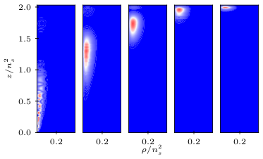
In Ref. Buchleitner et al. 2002 non-spreading wavepackets of a Rydberg electron are described. However, their formation has nothing to do with topological protection. They are related to the trapping of a Rydberg electron in a single well of an effective potential that is created by the resonant driving of the H atom. The mechanism of the formation of the localized states considered in this Letter is completely different. The localized states are edge states with localization length , where and are tunneling rates of an electron through the higher and lower barriers, respectively, of the effective potential in (2) Asbóth et al. 2016. The localization length can be much larger than the size of a single well of the effective potential in (2). Topological protection means that if we change the parameters of the effective model (2), can change but the localization phenomenon itself will not be broken, provided that the energy gap is not closed.
Topological molecules. Attractive interactions between charge particles allow atoms to form molecules. It is also possible to create bound states of atoms if the interaction potential between them changes in a disordered way as a function of their relative distances. Then, they can form the so-called Anderson molecules that are created due to destructive interference and the resulting Anderson localization Giergiel et al. 2018; Sacha 2020; Matus et al. 2021. Here we show that it is possible to realize bound states of atoms which have a topological origin. We will see that the description of two atoms with the interaction strength modulated in time can be reduced to the effective Hamiltonian where we can identify a center of mass degree of freedom described by the free particle-like Hamiltonian and the relative position degree of freedom described by the Hamiltonian (2). The edge states of the Hamitlonian (2) will correspond to the molecular bound states protected by topology.
Let us consider two atoms which are moving in the one-dimensional (1D) infinite well potential. For simplicity, we assume that they are the same atomic species but in different hyperfine states. The infinite well potential in 1D can be created experimentally if, in a 3D trap, with strong transverse confinement, two barriers are implemented that limit the motion of the atoms along the longitudinal direction Gaunt et al. 2013. At low kinetic energies, the interaction between atoms can be modeled by means of the contact Dirac delta potential with the strength proportional to the s-wave scattering length of the atoms. We assume that is modulated periodically in time by means of Feshbach resonance Chin et al. 2010 or confinement-induced resonance Olshanii 1998 so that the Hamiltonian of the system reads
| (7) |
where . We have used and as units of energy and length, respectively, where is the size of the potential well and is the mass of the atoms. For simplicity, we have used the same notation for the parameters of as in the case of a H atom, cf. (1), but now and are quantities proportional to the s-wave scattering length of the atoms. As previously, . In the units that we use, the motion of the atoms is limited between and due to the presence of the potential walls. Thus, the wavefunction vanishes if or equals 0 or .
To describe the system, it is sufficient to restrict to the subspace of symmetric combinations of the eigenstates of the noninteracting atoms, i.e. for and , where , because there is no interaction between the atoms in the antisymmetric subspace SM. We are interested in the resonant behavior of the system where and . Switching to the moving frame by means of the unitary transformation and averaging the resulting Hamiltonian over time, we arrive at the matrix of the quantum effective Hamiltonian that consists of independent blocks labeled with different values of . That is, in a given block the matrix elements of the read SM
| (9) | |||||
| (10) |
where . The position operators conjugate to the quantum numbers and are and , respectively. This effective description is valid in the subspace .
Apart from the last term, the matrix (10) is identical to the matrix of the quantized version of the classical effective Hamiltonian (2) calculated in the plane wave basis, , if the effective mass , and . Thus, the two-atom system behaves like a two-particle system whose center of mass position (conjugate to the momentum quantum number ) moves like a free particle [cf. the term in (10)] while the relative position can possess topologically protected edge states corresponding to the bound states of the particles. Particles prepared in an edge state form a topological molecule in which their relative position is described by a localized state that is protected by topology.
Our secular approximation approach allows us to identify parameters suitable for the realization of a topological molecule, but we are also able to describe the system exactly by numerical diagonalization of the Floquet Hamiltonian where is given in (7) Shirley 1965; Buchleitner et al. 2002; SM. The eigenstates of are called Floquet states which evolve with the same period as the period of and the corresponding eigenvalues are quasienergies of the system. The eigenstates of the effective Hamiltonian (10) also evolve periodically in time when we return to the laboratory frame, and they constitute a very good approximation of the exact Floquet eigenstates of .
In Fig. 3(a) we show the exact Floquet states, in the moving frame, that correspond to the edge states described above. The probability densities describing the position , which is conjugate to the quantum number , perfectly match the edge state probability densities obtained with the help of the effective Hamiltonian (10). It confirms that the atoms can form topologically protected bound states. When the system is observed in the laboratory frame, the signatures of the formation of the topological molecule are illustrated in Fig. 3(b). That is, the probability density for the atoms to be observed at reveals a periodic appearance of the localized edge state.
Conclusions. We have shown that topology is capable of protecting the states of the atomic constituents. A Rydberg electron can be represented by a localized wavepacket moving along a classical orbit, and such a localization is protected by topology. A similar mechanism is responsible for the formation of topological molecules — bound states of particles protected by topology.
We have considered the localization of a Rydberg electron on a Kepler orbit aligned along the static electric field direction. However, one may expect that the topological localization can also be observed on Kepler orbits with different shapes. That is, the static electric field allows one to control the shape of a stable Kepler ellipse Sacha, K. et al. 1998, and similar microwave fields as we have used here should lead to the topological localization of the electron on the ellipse. The experimental setup for realization of the phenomenon we predict can be very similar to the procedure used in Refs. Maeda and Gallagher 2004; Maeda and Gallagher 2007; Maeda et al. 2009; Wyker et al. 2012 where nonspreading Rydberg wavepackets were demonstrated.
Ultra-cold atoms in a quasi-1D squared well potential Gaunt et al. 2013 seem to be a suitable system for the realization of topological molecules. Two localized clouds of atoms can be pushed to motion, and if it is done at proper phase of the time periodic modulation of the strength of interactions between atoms, the clouds will be locked to a localized edge state of an effective topological model that describes the system SM. Modulation of the interaction strength can be done by means of the Feshbach resonance Chin et al. 2010 or the confinement-induced resonance in quasi–1D potentials Olshanii 1998; Haller et al. 2010.
Acknowlegement. This work was supported by the National Science Centre, Poland, through Projects: No. 2018/31/B/ST2/00349 (AEK), No. 2016/20/W/ST4/00314 and No. 2019/32/T/ST2/00413 (KG), QuantERA Programme No. 2017/25/Z/ST2/03027 (KS). KG acknowledges the support of the Foundation for Polish Science (FNP) and the support of the Polish National Agency for Academic Exchange Bekker Programme (BPN/BEK/2021/1/00339). XT acknowledges the support of the Foundation (Yucai project) from Guangxi Normal University. Some parts of our numerical schemes are based on the PETSc Balay et al. 2019; Balay et al. 1997 and SLEPc Hernandez et al. 2005 libraries. Numerical computations in this work were supported in part by PL-Grid Infrastructure.
References
- Nayak et al. (2008) C. Nayak, S. H. Simon, A. Stern, M. Freedman, and S. Das Sarma, Rev. Mod. Phys. 80, 1083 (2008), URL https://link.aps.org/doi/10.1103/RevModPhys.80.1083.
- Hasan and Kane (2010) M. Z. Hasan and C. L. Kane, Rev. Mod. Phys. 82, 3045 (2010), URL https://link.aps.org/doi/10.1103/RevModPhys.82.3045.
- Guo et al. (2013) L. Guo, M. Marthaler, and G. Schön, Phys. Rev. Lett. 111, 205303 (2013), URL https://link.aps.org/doi/10.1103/PhysRevLett.111.205303.
- Sacha (2015a) K. Sacha, Phys. Rev. A 91, 033617 (2015a), URL http://link.aps.org/doi/10.1103/PhysRevA.91.033617.
- Sacha (2015b) K. Sacha, Sci. Rep. 5, 10787 (2015b), URL https://www.nature.com/articles/srep10787.
- Sacha and Zakrzewski (2018) K. Sacha and J. Zakrzewski, Rep. Prog. Phys. 81, 016401 (2018), URL https://doi.org/10.1088/1361-6633/aa8b38.
- Guo and Liang (2020) L. Guo and P. Liang, New Journal of Physics 22, 075003 (2020), URL https://doi.org/10.1088/1367-2630/ab9d54.
- Sacha (2020) K. Sacha, Time Crystals (Springer International Publishing, Switzerland, Cham, 2020), ISBN 978-3-030-52523-1, URL https://doi.org/10.1007/978-3-030-52523-1.
- Guo (2021) L. Guo, Phase Space Crystals, 2053-2563 (IOP Publishing, 2021), ISBN 978-0-7503-3563-8, URL https://dx.doi.org/10.1088/978-0-7503-3563-8.
- Buchleitner et al. (2002) A. Buchleitner, D. Delande, and J. Zakrzewski, Physics reports 368, 409 (2002), URL http://www.sciencedirect.com/science/article/pii/S0370157302002703.
- Delande and Buchleitner (1994) D. Delande and A. Buchleitner, in , edited by B. Bederson and H. Walther (Academic Press, 1994), vol. 34 of Advances In Atomic, Molecular, and Optical Physics, pp. 85–123, URL http://www.sciencedirect.com/science/article/pii/S1049250X08600750.
- Bialynicki-Birula et al. (1994) I. Bialynicki-Birula, M. Kaliński, and J. H. Eberly, Phys. Rev. Lett. 73, 1777 (1994), URL https://link.aps.org/doi/10.1103/PhysRevLett.73.1777.
- Maeda and Gallagher (2004) H. Maeda and T. F. Gallagher, Phys. Rev. Lett. 92, 133004 (2004), URL http://link.aps.org/doi/10.1103/PhysRevLett.92.133004.
- Maeda and Gallagher (2007) H. Maeda and T. F. Gallagher, Phys. Rev. A 75, 033410 (2007), URL https://link.aps.org/doi/10.1103/PhysRevA.75.033410.
- Maeda et al. (2009) H. Maeda, J. H. Gurian, and T. F. Gallagher, Phys. Rev. Lett. 102, 103001 (2009), URL https://link.aps.org/doi/10.1103/PhysRevLett.102.103001.
- Wyker et al. (2012) B. Wyker, S. Ye, F. B. Dunning, S. Yoshida, C. O. Reinhold, and J. Burgdörfer, Phys. Rev. Lett. 108, 043001 (2012), URL https://link.aps.org/doi/10.1103/PhysRevLett.108.043001.
- Giergiel and Sacha (2017) K. Giergiel and K. Sacha, Phys. Rev. A 95, 063402 (2017), URL https://link.aps.org/doi/10.1103/PhysRevA.95.063402.
- Eiles et al. (2021) M. T. Eiles, A. Eisfeld, and J. M. Rost, arXiv e-prints arXiv:2111.10345 (2021), eprint 2111.10345.
- Lichtenberg and Lieberman (1992) A. Lichtenberg and M. Lieberman, Regular and chaotic dynamics, Applied mathematical sciences (Springer-Verlag, 1992), ISBN 9783540977452, URL https://books.google.pl/books?id=2ssPAQAAMAAJ.
- (20) See Supplemental Material where the details of the deriviation of the classical and quantum effective Hamiltonians and the discussion of robustness of the realization of the effective models are presented.
- Sacha, K. et al. (1998) Sacha, K., Zakrzewski, J., and Delande, D., Eur. Phys. J. D 1, 231 (1998), URL https://doi.org/10.1007/s100530050086.
- Su et al. (1979) W. P. Su, J. R. Schrieffer, and A. J. Heeger, Phys. Rev. Lett. 42, 1698 (1979), URL https://link.aps.org/doi/10.1103/PhysRevLett.42.1698.
- Asbóth et al. (2016) J. Asbóth, L. Oroszlány, and A. Pályi, A Short Course on Topological Insulators: Band Structure and Edge States in One and Two Dimensions, Lecture Notes in Physics (Springer International Publishing, 2016), ISBN 9783319256078, URL https://books.google.pl/books?id=RWKhCwAAQBAJ.
- Cooper et al. (2019) N. R. Cooper, J. Dalibard, and I. B. Spielman, Rev. Mod. Phys. 91, 015005 (2019), URL https://link.aps.org/doi/10.1103/RevModPhys.91.015005.
- Atala et al. (2013) M. Atala, M. Aidelsburger, J. T. Barreiro, D. Abanin, T. Kitagawa, E. Demler, and I. Bloch, Nature Physics 9, 795 (2013), ISSN 1745-2481, URL https://doi.org/10.1038/nphys2790.
- Meier Eric J. et al. (2016) Meier Eric J., An Fangzhao Alex, and Gadway Bryce, Nature Communications 7, 13986 (2016), URL https://www.nature.com/articles/ncomms13986#supplementary-information.
- St-Jean et al. (2017) P. St-Jean, V. Goblot, E. Galopin, A. Lemaître, T. Ozawa, L. Le Gratiet, I. Sagnes, J. Bloch, and A. Amo, Nature Photonics 11, 651 (2017), ISSN 1749-4893, URL https://doi.org/10.1038/s41566-017-0006-2.
- Giergiel et al. (2019) K. Giergiel, A. Dauphin, M. Lewenstein, J. Zakrzewski, and K. Sacha, New Journal of Physics 21, 052003 (2019), URL https://doi.org/10.1088/1367-2630/ab1e5f.
- (29) The chosen Fourier components allow one to realize a barrier in the effective model (2). This barrier can be realized in many different ways, see SM. The small parameter breaks the reflection symmetry of the potential in the effective SSH model — if such a symmetry was present, the edge states would be superpositions of the localized wavepackets presented in Fig. 1(b).
- Giergiel et al. (2018) K. Giergiel, A. Miroszewski, and K. Sacha, Phys. Rev. Lett. 120, 140401 (2018), URL https://link.aps.org/doi/10.1103/PhysRevLett.120.140401.
- Matus et al. (2021) P. Matus, K. Giergiel, and K. Sacha, Phys. Rev. A 103, 023320 (2021), URL https://link.aps.org/doi/10.1103/PhysRevA.103.023320.
- Gaunt et al. (2013) A. L. Gaunt, T. F. Schmidutz, I. Gotlibovych, R. P. Smith, and Z. Hadzibabic, Phys. Rev. Lett. 110, 200406 (2013), URL https://link.aps.org/doi/10.1103/PhysRevLett.110.200406.
- Chin et al. (2010) C. Chin, R. Grimm, P. Julienne, and E. Tiesinga, Rev. Mod. Phys. 82, 1225 (2010), URL https://link.aps.org/doi/10.1103/RevModPhys.82.1225.
- Olshanii (1998) M. Olshanii, Phys. Rev. Lett. 81, 938 (1998), URL https://link.aps.org/doi/10.1103/PhysRevLett.81.938.
- Shirley (1965) J. H. Shirley, Phys. Rev. 138, B979 (1965), URL https://link.aps.org/doi/10.1103/PhysRev.138.B979.
- Haller et al. (2010) E. Haller, M. J. Mark, R. Hart, J. G. Danzl, L. Reichsöllner, V. Melezhik, P. Schmelcher, and H.-C. Nägerl, Phys. Rev. Lett. 104, 153203 (2010), URL https://link.aps.org/doi/10.1103/PhysRevLett.104.153203.
- Balay et al. (2019) S. Balay, S. Abhyankar, M. F. Adams, J. Brown, P. Brune, K. Buschelman, L. Dalcin, A. Dener, V. Eijkhout, W. D. Gropp, et al., Tech. Rep. ANL-95/11 - Revision 3.12, Argonne National Laboratory (2019), URL https://www.mcs.anl.gov/petsc.
- Balay et al. (1997) S. Balay, W. D. Gropp, L. C. McInnes, and B. F. Smith, in Modern Software Tools in Scientific Computing, edited by E. Arge, A. M. Bruaset, and H. P. Langtangen (Birkhäuser Press, 1997), pp. 163–202.
- Hernandez et al. (2005) V. Hernandez, J. E. Roman, and V. Vidal, ACM Trans. Math. Softw. 31, 351 (2005), ISSN 0098-3500, URL http://doi.acm.org/10.1145/1089014.1089019.
- Guo and Marthaler (2016) L. Guo and M. Marthaler, New Journal of Physics 18, 023006 (2016), URL http://stacks.iop.org/1367-2630/18/i=2/a=023006.
- Tanzi et al. (2018) L. Tanzi, C. R. Cabrera, J. Sanz, P. Cheiney, M. Tomza, and L. Tarruell, Phys. Rev. A 98, 062712 (2018), URL https://link.aps.org/doi/10.1103/PhysRevA.98.062712.
I Supplemental Materials
In this Supplemental Material, we derive the classical and quantum effective Hamiltonians and discuss robustness of the realization of the effective models.
II Hydrogen atom
We consider a H atom in the presence of static electric and linearly polarized microwave fields which in the atomic units is descrbed by the Hamiltonian
| (S1) |
where
| (S2) |
, and are the strength of the electric field and the amplitudes of the microwaves, respectively, and is an integer number.
Let us begin with the classical description. In terms of the so-called action-angle variables Lichtenberg and Lieberman 1992; Buchleitner et al. 2002, the Hamiltonian (S1) reads
| (S4) | |||||
where
| (S5) | |||||
| (S6) | |||||
| (S7) |
is the eccentricity of a Kepler orbit of the Rydberg electron, and , denote the Bessel functions and their derivatives, respectively. We have assumed that the projection of the angular momentum of the electron on the axis (which is a constant of motion) is zero. The principal action is the classical analogue of the principal quantum number and the conjugate angle describes the position of the electron in a Kepler orbit. The angular momentum is conjugate to which is the angle between the major axis of a Kepler ellipse and the axis. We are going to describe the electron close to the resonant orbit where the microwave frequency is times higher than the frequency of the unperturbed electronic motion given by [ is the same as in (S2)]. If we switch to the moving frame,
| (S8) |
then for , where , all dynamical variables are slowly varying in the limit of the weak perturbation and we may average the Hamiltonian over time keeping , , and fixed which results in the secular effective Hamiltonian Lichtenberg and Lieberman 1992
| (S14) | |||||
The static electric field controls the shape of stable resonant orbits Sacha, K. et al. 1998. If the static field dominates over the microwave fields, the stable orbit is the Kepler ellipse degenerate into a line where the resonantly driven electron is moving with the period along the direction of the electric field vector with and , see Fig. S1. Then electronic motion close to such a resonant orbit can be described by a simplified version of ()
| (S16) |
where we set and and expanded the first two terms of () in the Taylor series up to the second order in , which is small if we choose initial conditions of the electron close to the resonant orbit. The effective mass , , and . The effective Hamiltonian (S16) is the basis of the description of the topological behavior we analyze in the Letter, and its validity can be tested with the help of the exact numerical integration of the classical equations of motion. In Fig. S2 we show the phase space portrait generated by (S16) and the corresponding stroboscopic map obtained by numerically solving the equations of motion generated by the exact Hamiltonian (S1) for and . The agreement is perfect, therefore we may be sure that the exact dynamics reveals the topological behavior we are after.


Quantum description of the electron moving resonantly on the Kepler orbit aligned along the electric field direction can be performed either by quantizing the classical effective Hamiltonian (S16) or by deriving an effective Hamiltonian fully quantum mechanically. The latter is done by switching to the moving frame with the help of the unitary transformation [which is the quantum analogue of the classical canonical transformation to the moving frame (S8)], and averaging the resulting Hamiltonian over time which leads to
| (S19) | |||||
where is the hydrogenic eigenstate with the principal quantum number (), the total angular momentum and the projection of the angular momentum on the axis equaled zero. Comparison of the resonant spectra obtained by diagonalization of () and (S16) is presented in Fig. 1 in the Letter. The results match each other very well, which, together with the agreement between the exact and secular classical descriptions (cf. Fig. S2), proves the consistency of the approach we use.
At the end of this section let us discuss robustness of the topologically protected localization of a Rydberg electron.
The role of the driving function is to create a localized barrier in the effective potential in Eq. (S16). Without , there is no edge in the system and no topologically protected localized edge states can be observed. There are basically two requirements that must meet: (i) the resulting barrier must be localized on a length scale much shorter than the size of the entire crystalline structure and (ii) the barrier height must be larger than the width of the energy bands of the effective model (S16). The latter condition ensures that the presence of the barrier results in open boundary conditions in our crystalline structure, which implies that there is an edge in the system.
The topological localization of a Rydberg electron is stable with respect to different choices of provided the conditions described above are satisfied. From the experimental point of view, it is important to use with the smallest possible number of Fourier components . The function used in Fig. 1 in the Letter consists of with up to , but even if we choose , the shape of the edge states does not change noticeably, see Fig. S3. In addition, the precise functional form of is not important. In Fig. S3 we present different choices of , the resulting and the probability densities of one of the edge states.
In the experiment, to realize the effective model (S16) one has to apply a time-periodic driving with frequencies and . This is a critical requirement which, however, can be easily fulfilled in the experiment because having the driving with the frequency its second harmonic with the frequency can be generated.
The frequency satisfies the resonant condition but does not necessarily have to be exactly equal to . If is different from , then the tunneling amplitudes in the resulting Su-Shrieffer-Heeger (SSH Su et al. 1979; Asbóth et al. 2016) model acquire complex phases Guo and Marthaler 2016. However, these phases can be eliminated by proper redefinition of the phases of the basis states if the barrier potential is present and the open boundary conditions are realized.
It is not necessary to realize the effective model (S16) with exactly the same parameters as presented in the Letter. The localization of a Rydberg electron is robust, provided that one realizes the effective model in the topologically non-trivial regime. The localization length of the edge states can change with a change in the parameters of the system, but the localization phenomenon itself is robust if the gap between the bands is not closed.
III Topological molecules
In the Letter we introduce the Hamiltonian
| (S21) |
which describes motion of two different atoms (the same atomic species but in different hyperfine states) in the squared potential well whose size is . We use
| (S22) |
as units of energy and length, respectively, where is the size of the potential well and is the mass of the atoms. The strength of contact interactions between atoms is periodically modulated in time
| (S23) |
where is given in (S2). We are interested in the motion of the atoms that is resonant with the time-periodic modulation of the interaction strength .
A suitable basis for the quantum description of the atoms is formed by the eigenstates of the non-interacting atoms,
| (S24) |
For antisymmetric combinations of these states, we obtain
| (S25) |
It means that the interaction between the atoms can only take place if they are prepared in the symmetric combinations of (S24), i.e.
| (S26) | |||||
| (S27) |
and thus we may restrict to such a subspace only.
The eigenstates of the effective Hamiltonian () are a secular approximation of the exact Floquet states. The resonant motion of the atoms means that and where is an integer and the same as in (S2). In order to derive an effective quantum Hamiltonian that can describe the resonant behavior of the atoms we switch to the moving frame by means of the unitary transformation and average the resulting Hamiltonian over time. Introducing the quantum numbers and , the matrix elements of the obtained effective Hamiltonian read
| (S30) | |||||
This effective Hamiltonian, which is valid for , describes a two-particle system whose center of mass degree of freedom behaves like a free particle, i.e. there is only kinetic energy given by . The relative position degree of freedom of the particles (corresponding to the momentum quantum numbers ) behaves in the same way as the Rydberg electron described in the previous section. Indeed, the matrix elements () are identical to the matrix elements of the quantized version of the classical effective Hamiltonian (S16) calculated in the plane wave basis, , if , and . Thus, the two-particle system can be prepared in a state where the relative position degree of freedom forms a bound state corresponding to a localized edge state, i.e. a molecule which is protected by topology.
Eigenstates of the effective Hamiltonian () are secular approximation of the exact Floquet states of the system in the moving frame. The latter are eigenstates of the Floquet Hamiltonian which, in the moving frame, reads
| (S32) |
where is given in (S21) Shirley 1965. In order to obtain the exact Floquet states we diagonalize the Floquet Hamiltonian in the Hilbert space extended by the Fourier states where , i.e. diagonalize the matrix
| (S33) | |||||
| (S34) |
In Fig. S4 a comparison of the spectra obtained by diagonalization of the exact Floquet Hamiltonian () and the effective Hamiltonian () is presented. If is sufficiently large, we obtain perfect agreement. It means that the phenomena that we can predict with the help of are reproduced in the exact description of the system.
Topological molecules can be realized in ultra-cold atoms. To give a flavor of the experimental parameters, let us consider the following example. Assume that two 39K atoms in the two different hyperfine states, and , are trapped in the quasi-1D box potential Gaunt et al. 2013 of longitudinal size of m. The strong transverse confinement is realized by means of the harmonic potential with the frequency kHz. The atoms are initially prepared in the Gaussian wavepackets of the width m located on the opposite sides of the quasi-1D box potential (i.e., at m and m) and with the average velocities mm/s. To observe one of the edge states corresponding to in Fig. S4, the frequency and the maximal amplitude of the inter-species s-wave scattering length modulation [cf. Eq. (S23)] have to be Hz and nm, respectively. This modulation can be achieved by periodic changes of an external magnetic field in time in the vicinity of the Feshbach Resonance at 113.76 G Tanzi et al. 2018. If the Gaussian wavepackets are prepared at , then their squared overlap with one of the edge states is 0.4 and in the course of time evolution of the system one will observe signatures of the formation of the topological molecule, see Fig. S5. Note that the intial product of the Gaussian states (which is the easiest to prepare experimentally) belongs both to the symmetric and antisymmetric subspaces, cf. Eqs. (S25)-(S27). Consequently, its maximal possible squared overlap with the edge state is 0.5 and the squared overlap of 0.4 in our example is close to this maximal value. The part of the initial state that belongs to the antisymmetric subspace evolves like for non-interacting particles and consequently it spreads over the entire box and forms a background of the probability density shown in Fig. S5. On this background, a localized peak is clearly visible which is the signature of the topological molecule.