Unitary-Precoded Single-Carrier Waveforms for High Mobility: Detection and Channel Estimation

Let ${\bf X}\in\mathbb{C}^{M\times N}$ be the 2-D information symbol matrix. Let ${\bf X}_{\rm FT}\in\mathbb{C}^{M\times N}$ be the frequency-time samples generated by precoding the information symbols in ${\bf X}$. ${\bf X}_{\rm FT}(m,n)$ represents the precoded data sample transmitted in the $m$-th sub-carrier of the $n$-th time slot, where $m=0,\ldots,M-1$ and $n=0,\ldots,N-1$. Let $\mathbf{\widetilde{\text{$\bf X$}}}\in\mathbb{C}^{M\times N}$ be the delay-time samples generated from the time-frequency samples using the Heisenberg transform as

where ${\bf G}_{\rm TX}$ is the pulse shaping waveform at the transmitter. We assume the rectangular pulse shaping waveform in this paper, i.e., ${\bf G}_{\rm TX}={\bf I}_{M}$. The operation is (1) is the conventional OFDM modulator. The $NM\times 1$ time domain samples are generated by vectorizing the delay-time domain samples as

The time-domain signal are divided into $N$ blocks ${\bf s}_{n}$ of size $M$ as ${\bf s}=[{\bf s}_{0}^{\rm T},\ldots,{\bf s}_{N-1}^{\rm T}]^{\rm T}$ and finally a guard interval of length $L_{\rm G}$ is added to each time domain block in ${\bf s}$ to avoid inter-block interference. The guard intervals can either be filled with a cyclic prefix (CP) or zero-padding (ZP).

The generalized 2-D unitary precoding can be written in matrix form as

where ${\bf U}_{\rm F}\in\mathbb{C}^{M\times M}$ and ${\bf U}_{\rm T}\in\mathbb{C}^{N\times N}$ are the precoding matrices along the frequency and time domain, respectively.

In [3], it was proved that any orthogonal 2-D transformation with constant modulus basis functions operating on the entire frequency-time domain allows the receiver to exploit maximum frequency-time diversity in doubly-selective channels. This implies that, in terms of error performance, the best choice for ${\bf U}_{\rm F}$ and ${\bf U}_{\rm T}$ are unitary transforms, such as DFT and WHT. The precoding matrices ${\bf U}_{\rm F}$ and ${\bf U}_{\rm T}$ for different modulation schemes are listed in Table I.

A 2-D unitary precoding in the frequency-time domain may increase the complexity of transceiver modulation and demodulation. One way to mitigate this complexity is by restricting the unitary transformation along the frequency domain to the FFT, i.e., ${\bf U}_{\rm F}={\bf F}_{M}$,

This simplifies the Heisenberg transform in (1) as (assuming practical rectangular pulse shaping waveforms):

Now, (5) can be considered as a precoding along the time dimension of the delay-time domain, i.e., the rows of $\mathbf{\widetilde{\text{$\bf X$}}}$. The time-domain signal is then generated as

The operations in (5) and (6) can be combined as

for $m=0,\ldots M-1$ and $k=0,\ldots,N-1$. This 1-D unitary precoding can still achieve maximum time-frequency diversity similar to a 2-D unitary precoding in the frequency-time domain, but with much lower modulation/demodulation complexity. For ${\bf U}_{\rm T}={\bf F}_{N}^{{\dagger}}$, the operation in (7) is known in the literature as the inverse discrete Zak transform (IDZT) and is equivalent to the OTFS transmitter for rectangular pulse shaping waveforms, [8, 9].

Let ${\bf X}\in\mathbb{C}^{M\times N}$ be the 2-D information symbols. The transmitted information symbol matrix ${\bf X}$ and the delay-time samples are vectorized as

Let ${\bf P}$ be the row-column interleaver matrix which writes the $NM$ samples column-wise into a $N\times M$ matrix and reads the elements out row-wise. The time-domain samples can then be generated using (7) as

where ${\bf U}_{\rm T}$ is the precoding matrix along the time-domain given for different waveforms in the literature as given in Table I. The time domain samples are then pulse shaped, digital to analog converted and transmitted into the wireless medium as $s(t)$ at a carrier frequency $f_{c}$.

Consider a channel with $P$ paths, where $h_{i}$, $\tau_{i}$ and $\nu_{i}$ are the propagation gain, delay and Doppler-shift associated with $i$-th path. We assume that the delay-Doppler channel response is given by

The delay-time channel in terms of the delay-Doppler response is given as

The received time-domain signal can then be written as

where $w(t)$ is the AWGN noise signal. The equivalent discrete-time channel is obtained by sampling the received time-domain waveform at $M\Delta f$ Hz, is given as

where $\tau=l/M\Delta f$, $t=q/M\Delta f$ and $\mathcal{L}$ denotes the set of discrete integer delay taps. The entries of $\mathbf{\bar{\text{$g$}}}[l,q]$ is given as

where $z=e^{\frac{j2\pi}{NM}}$, $l_{i}=\frac{\tau_{i}}{M\Delta f}$ and $\kappa_{i}=\frac{\nu_{i}}{NT}$ are the normalized delay and normalized Doppler-shift associated with the $i$-th path. We assume that the normalized delays $l_{i}$ are integers.

The transmitter operations are then reversed at the receiver. The delay-time received samples are obtained by folding the received signal ${\bf r}$ into a $M\times N$ matrix by filling it column-wise.

The received information symbols can then be obtained as

The operations in (15) and (16) can be combined as

Note that for ${\bf U}_{\rm T}={\bf F}_{N}^{{\dagger}}$, the operation in (17) is known in the literature as the discrete Zak transform (DZT) and is equivalent to the OTFS receiver for rectangular pulse shaping waveform, [8, 9]. Let the received 2-D symbol matrices ${\bf Y}$ and $\mathbf{\widetilde{\text{$\bf Y$}}}$ be vectorized as

The received vector can then be written in terms of the transmitted vector as

The input-output relation in (14) can be written in the matrix form as

where ${\bf G}$ is the time-domain channel matrix with a band width of $l_{\rm max}+1$ with entries: ${\bf G}[q,q-l]=\bar{g}[l,q]\text{ for }q\geq l$. Substituting (9) and (19) in (20), we get the input-output relation between the transmitted and received information symbols:

where ${\bf z}=({\bf I}_{M}\otimes{\bf U}_{T}^{{\dagger}})\cdot({\bf P}^{\rm T}\cdot{\bf w})$ is the AWGN noise and the channel matrix

For fair comparison with the traditional OFDM modulation scheme, we use the single tap frequency domain equalizer for USC waveforms. The received time-frequency samples can be obtained by the $M$-point FFT operation on the received time domain blocks

as in a standard OFDM receiver. We can then equalize each block in parallel as

for $n=0,\ldots,N-1$ and the frequency domain channel coefficients for each time-domain block are given by

where ${\rm diag}[{\bf A}]$ denotes the column vector containing the diagonal elements of the square matrix ${\bf A}$. The information symbol estimates in the delay-sequency domain can then be obtained by the $M$-point IFFT operation on the time-frequency domain estimates $\mathbf{\bar{\text{$\bf s$}}}_{n}$ followed by the $N$-point WHT as

Fig. 1 shows the QPSK BER performance of USC schemes compared with SC and OFDM modulation at a SNR of 20 dB for different speeds. We consider three different USC waveforms with DFT (OTFS). WHT (OTSM) and DCT. It can be observed that all the USC waveforms offer better performance as compared to OFDM and SC. However, as expected, the time-frequency single tap equalizer performance degrades in the presence of significant Doppler due to significant inter-carrier interference.

The frequency-domain equalizer performance, similar to OFDM, degrades in the presence of high Doppler spread channels (see Fig. 1). In this section we present a block-wise time-domain MMSE equalizer that can provide better performance in the case of time-varying channels. The MMSE equalizer will act as a baseline to compare the performance of the iterative detection methods we present later.

For the input-output relation in (28), the MMSE estimate of the time-domain samples,

The information symbols can then be estimated from the delay-time samples as

The time-domain MMSE equalizer offers good performance, but at the cost of high complexity. To reduce the complexity, we present an iterative detector based on the well known Gauss Seidel (GS) method, [10]. However, different from the traditional method, the GS iteration in this case is done on the matched filtered channel matrix blocks ${\bf R}_{n}={\bf G}^{{\dagger}}_{n}\cdot{\bf G}_{n}$. The matrix input-output relation in (28) after the matched filtering operation can be written as

where ${\bf R}_{n}={\bf G}^{{\dagger}}_{n}\cdot{\bf G}_{n}$, ${\bf z}_{n}={\bf G}^{{\dagger}}_{n}\cdot{\bf r}_{n}$ and $\mathbf{\bar{\text{$\bf w$}}}_{n}={\bf G}^{{\dagger}}_{n}\cdot{\bf w}_{n}$. The GS method is used to iteratively find the least squares solution

of the $M$-dimensional linear system of equations in (35).

Let ${\bf D}_{n}$ and ${\bf L}_{n}$ be the matrix containing the diagonal elements and the strictly lower triangular elements of the matched filter matrix ${\bf R}_{n}$. From [10], the GS iterative method for finding the estimate of ${\bf s}_{n}$ in each iteration is given as

where ${\bf T}_{n}\in\mathbb{C}^{M\times M}$ is the GS iteration matrix. The vector $\hat{\bf s}_{n}^{(i)}\in\mathbb{C}^{M\times 1}$ represents the estimate of the transmitted time-domain samples of the $n$-th block in the $i$-th iteration. The information symbols in the $i$-th iteration is then given as

where $\mathcal{D}(.)$ denotes the decision function replacing all the elements of the input with the nearest QAM symbol. The hard decision estimates are transformed back to the time domain to update the time domain estimate to be used in the next iteration.

where $\delta$ is the relaxation parameter to improve the detector convergence for higher modulation schemes like 64-QAM, [10, 8]. As initial estimate to the iterative detection, we can chose either ${\bf X}^{(0)}={\bf 0}$ or the single-tap solution in (32) yielding faster convergence. Note that the complexity of this algorithm can be significantly reduced by taking advantage of the sparsity of the matrices ${\bf G}_{n}$ and ${\bf T}_{n}$. It is shown in [8], that a delay-time version of this algorithm for OTFS has complexity $O(NML)$, where $L$ is the number of distinct channel delays. The same implementation can be straightforward extended to other USC waveforms.

The hardware platform is based on National Instruments universal radio software peripheral (USRP) software defined radio reconfigurable device (NI-USRP-2954R) designed by Ettus Research [12]. A Tx or Rx terminal is implemented with an USRP-2954R connected to a host PC running the National Instruments LabView using PCIe Express x4. The software is based on LabView 2020. We follow the OTFS SDR modem experimental setup described in [11] with the USC experiment parameters listed in Table II.

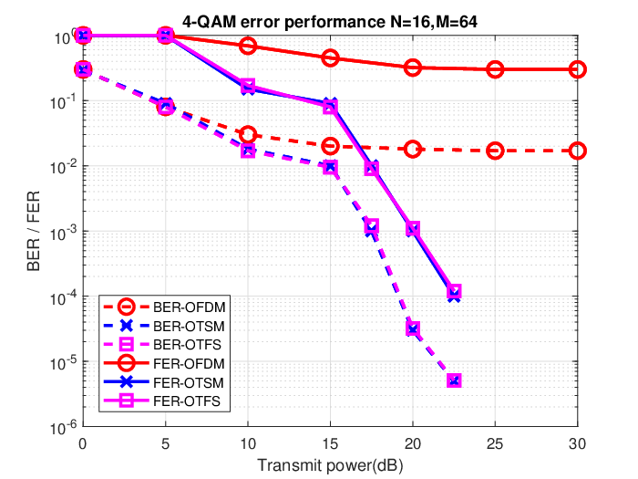
Fig. 6 presents the BER and FER performance of USC with DFT (OTFS) and WHT (OTSM) unitary matrices compared with OFDM in a real-time indoor channel using the NI USRP-2954 SDR platform. The OFDM frame of bandwidth $B=2$ MHz is generated according to the IEEE 802.11ac standard for WiFi using 48 out of 64 sub-carriers for data transmission and the rest for pilot and null symbols. The pilot overhead in USC waveforms is generated with a ZP of $L_{\rm G}=16$ samples to match the spectral efficiency of above OFDM. The information bits are encoded using a convolutional code of rate $R=1/2$. At the Rx the single-tap equalizer in Section IV-A is used for low-complexity detection and, the channel estimation method is given in Section III.

An instance of the received 2-D pilot magnitude in the indoor channel measured using the SDR is shown in Figs. 4 and 5 for OTFS and OTSM for a pilot transmitted at $(m_{\rm p},n_{\rm p})=(3,0)$. It can be observed that the delay-Doppler domain channel is more localized than the delay-sequency channel. However, the pilot energy is still leaked to all the Doppler bins due to fractional Doppler. Therefore, the entire Doppler axis needs to be reserved for the guard symbols to avoid interference with data. From Fig. 6, both both OTFS and OTSM offer better performance than OFDM in the indoor channel.

One reason for a high error floor in OFDM is due to the lack of CFO compensation at the receiver. OTSM, similar to OTFS, is more robust to CFO as compared to OFDM. Due to the significantly lower complexity of the WHT compared to the DFT and other unitary matrices, Moreover, if the information symbols are integers, the time domain samples after applying the WHT resulting in the least quantization error at the transmitter for the same DAC resolution. Due to above reasons, OTSM can be considered a more energy-efficient waveform than OFDM and OTFS for next-generation wireless channels.

References

- [1] R. Hadani, S. Rakib, M. Tsatsanis, A. Monk, A. J. Goldsmith, A. F. Molisch, and R. Calderbank, “Orthogonal time frequency space modulation,” in Proc. IEEE Wireless Commun. Netw. Conf. (WCNC), San Francisco, CA, USA, Mar. 2017.
- [2] Y. Hong, T. Thaj and E. Viterbo, Delay-Doppler Communications: Principles and Applications, Academic Press, 2022, ISBN:9780323850285
- [3] T. Zemen, M. Hofer, D. Löschenbrand and C. Pacher, “Iterative Detection for Orthogonal Precoding in Doubly Selective Channels,” in Proc. 2018 IEEE 29th Annu. Int. Symp. Personal Indoor and Mobile Radio Commun. (PIMRC), Bologna, 2018.
- [4] T. Thaj and E. Viterbo, “Orthogonal Time Sequency Multiplexing Modulation” in Proc. IEEE Wireless Commun. Netw. Conf., pp. 1-7, 2021
- [5] T. Thaj, E. Viterbo and Y. Hong, “Orthogonal Time Sequency Multiplexing Modulation: Analysis and Low-Complexity Receiver Design” in IEEE Trans. on Wireless Commun., 2021, doi: 10.1109/TWC.2021.3088479.
- [6] D. S. Stoffer, “Walsh-Fourier Analysis and Its Statistical Applications,” J. American Statistical Association, vol. 86, no. 414, pp. 461–479.
- [7] P. Raviteja, K. T. Phan, and Y. Hong, “Embedded Pilot-Aided Channel Estimation for OTFS in Delay–Doppler Channels,” IEEE Trans. Veh. Technol., vol. 68, no. 5, pp. 4906-4917, May 2019.
- [8] T. Thaj and E. Viterbo, “Low Complexity Iterative Rake Decision Feedback Equalizer for Zero Padded OTFS Systems,” IEEE Trans. on Veh. Tech., Dec 2020. doi: 10.1109/TVT.2020.3044276
- [9] S. K. Mohammed,“Derivation of OTFS Modulation From First Principles.” in IEEE Trans. on Veh. Tech., vol. 70, no. 8, pp. 7619-7636, Aug. 2021, doi: 10.1109/TVT.2021.3069913.
- [10] A. Björck, Numerical Methods for Least Squares Problems, SIAM, 1996. doi: 10.1137/1.9781611971484
- [11] T. Thaj and E. Viterbo, “OTFS Modem SDR Implementation and Experimental Study of Receiver Impairment Effects,” in 2019 IEEE Int. Conf. on Commun. Workshops, pp. 1-6, 2019, doi: 10.1109/ICCW.2019.8757167.
- [12] USRP-2954 Specifications - National Instruments, Available online: https://www.ni.com/pdf/manuals/375725c.pdf
- [13] “LTE Evolved Universal Terrestrial Radio Access (E-UTRA); Base Station (BS) radio transmission and reception,” 3GPP TS 36.104 version 8.6.0 Release 8, Jul. 2009, ETSI TS. doi: 10.1109/MCOM.2009.4752682