A New Algebraic Approach for String Reconstruction from Substring Compositions
An earlier version of this paper was presented in part at the 2022 IEEE International Symposium on Information Theory [DOI: 10.1109/ISIT50566.2022.9834531]. This work was supported by the National Science Foundation under grant CCF–1941633.
Abstract
In this paper, we propose a new algorithm for the problem of string reconstruction from its substring composition multiset. Motivated by applications in polymer-based data storage for recovering strings from tandem mass-spectrometry sequencing, the algorithm exploits the equivalent polynomial formulation of the problem. We characterize sufficient conditions for a length binary string that guarantee the string’s reconstruction time complexity to be bounded polynomially as . This improves the time complexity of the reconstruction process compared to the complexity of the algorithm by Acharya et al. for this problem [1]. Moreover, the sufficient conditions on binary strings that guarantee reconstruction in polynomial time are more general than the conditions for the algorithm by Acharya et al. This is used to construct new codebooks of reconstruction codes that have efficient encoding procedures, and are larger, by at least a linear factor in size, compared to the previously best known construction by Pattabiraman et al. [2].
I Introduction
Recent years have seen an explosion in the amount of data created globally [3]. The volume of data generated, consumed, copied, and stored is projected to reach more than 180 zettabytes by 2025. In 2020, the total amount of data generated and consumed was 64.2 zettabytes [4]. But traditional digital data storage technologies such as SSDs, hard drives, and magnetic tapes are approaching their fundamental density limits and would not be able to keep up with the increasing memory needs [5].
Several molecular paradigms with significantly higher storage densities have been proposed recently [6, 7, 8, 9, 10, 11, 12, 13, 14, 15, 16, 17]. Molecules with a structure consisting of different smaller molecules (monomers) joined together in sequences are called polymers. If different types of molecules denote different alphabets, then a polymer with a linear arrangement of these molecules, i.e., a polymer string, can be treated as a sequence of alphabets. DNA is one promising data storage medium which has generated significant interest in the data storage research community. However, DNA has several scalability constraints including an expensive synthesis and sequencing process which prevent large-scale commercialization. Furthermore, DNA is prone to a diverse type of errors such as mutations within strands, or loss of strands due to breakage or degradation that could lead to potential decoding errors or even complete loss of information [10].
This has led researchers to search for alternatives in other synthetic polymers. For example, synthetic proteins (which are polymers of amino acids) are emerging as a potential alternative with data being stored using peptide sequences for the first time in 2021 [6]. Compared to DNA and other types of polymers, proteins offer several advantages for data storage, including higher stability of some proteins than DNA [18], and availability of a larger set of possible monomers ( amino acids are observed in natural proteins).
In synthetic polymer strings, monomer units of different masses, which represent the two bits and , are assembled into user-determined readable sequences. A common family of technological methods for reading amino-acid sequences (and other bio-polymers) is mass spectrometry [19]. Mass spectrometers take a large number of identical polymer strings, randomly break the polymer into substrings, and analyze the resulting mixture. The mass sequencing spectrum obtained gives us the mass and frequency of each contiguous molecular substring. The process of recovering a molecular string from its mass sequencing spectrum is modeled into the problem of reconstructing a string from the multiset of the compositions of its contiguous substrings.
The class of problems of reconstructing a string from substring information usually falls under the general framework of the string reconstruction problems. Due to their relevance in modelling molecular storage frameworks, the list of recent work in string reconstruction problems has grown rapidly [20, 21, 22, 23, 24, 25, 26, 27, 1, 28]. The problem of string reconstruction from its substring compositions was first introduced in [29] and [1]. The main results from [1] assert that binary strings of length , one less than a prime, and one less than twice a prime are uniquely reconstructable, from their substring composition multiset, up to reversal. The authors of [1] also introduced a backtracking algorithm for reconstructing a binary string from its substring composition multiset, and provide sufficient conditions for reconstructability of a binary string using the proposed algorithm in [1] without the need for backtracking (lemma 3). In the case of no backtracking, this algorithm has a time complexity of . Note that in the case of backtracking, there is no guarantee that the time complexity will remain bounded polynomially with . Relying on this reconstruction algorithm, the works of [2], [30] and [31] viewed the problem from a coding theoretic perspective. They proposed coding schemes that are capable of correcting a single mass error and multiple mass errors, respectively, and can be reconstructed by the reconstruction algorithm without backtracking.
The problem formulation in [1], and subsequently in[2], relies on the two following assumptions: a) One can uniquely infer the composition (number of monomers of each type) of a polymer from its mass; and b) The masses of all the substrings of a polynomial are observed with identical frequencies. In this work, we also rely on these assumptions.
In the context of combinatorics, the problem is closely related to the turnpike problem, also known as the partial digest problem, where the locations of highway exits need to be recovered from the multiset of their interexit distances. In [1], the authors showed that the problem of string reconstruction from its composition multiset can be reduced to an instance of the turnpike problem.
In this paper, we propose a new algorithm to reconstruct the set of binary strings with a given multiset of substring compositions. The proposed algorithm relies on on the algebraic properties of the equivalent bivariate polynomial formulation [1] of the problem. The algorithm finds the coefficients of the corresponding polynomial in a manner that reconstructs the binary string from both ends progressing towards the center. We show that the time complexity of the reconstruction process is reduced with our proposed algorithm compared to the combinatorial algorithm proposed in [1]. However, in general, a drawback of such algorithms is that they may need backtracking which can lead to reconstruction complexity that grows exponentially with the length , in a worst case scenario. Therefore, we provide algebraic conditions on binary strings that are sufficient to guarantee unique reconstruction by the proposed algorithm without backtracking, that is in time complexity. The algorithm naturally allows parallel implementation and has an reconstruction latency. Furthermore, the no backtracking condition of our algorithm is more general than that of the algorithm in [1]. This in particular implies that the reconstruction code introduced in [2] is reconstructable by our reconstruction algorithm without backtracking. We also improve the time complexity in the case of backtracking. These results are specifically discussed in remark 9, remark 12, and remark 13.
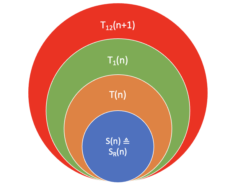
In section IV, properties of one-dimensional random walks are leveraged to explicitly characterize the set of binary strings that can be reconstructed by the algorithm in [1] without backtracking. In particular, we define this reconstruction code to be and show a bijection between ; and -dimensional positive -step walks starting from the origin. Using this bijection we propose efficient encoding and decoding procedures for and show an equivalence between and the reconstruction code introduced in [2] . We further extend this codebook to propose a new reconstruction code by expanding codebooks of different sizes in certain specified ways followed by taking a union of them. The size of is shown to be linearly larger than , and equivalently . Furthermore, it is shown that both, the codebook (and equivalently ), and the codebook are reconstructable by our proposed reconstruction algorithm in time. Finally, exploiting the more general sufficient conditions, we slightly modify the proposed algorithm, to introduce larger codebooks , and . A comparison of the rates and redundancies of the different coding schemes is presented in figures 3 and 3.
The rest of this paper is organized as follows. We describe the problem setting, preliminaries, and relevant previous work in Section II. Then, we describe the new reconstruction algorithm in Section III. In Section IV, we present the new reconstruction code. Finally, we discuss concluding remarks and future research directions in Section V.
II Preliminaries
In this section, we first establish some useful terminology and thereupon formally describe the problem being addressed in this paper. We then recap the results of [1], and [2] which give the relevant background and provide a simple polynomial characterizing of the problem.
II-A Problem Formulation
Let be a binary string of length and let denote the contiguous substring of , where . We will say that a substring has the composition where and denote the number of and in the substring respectively. The composition multiset of a sequence is the multiset of compositions of all contiguous substrings of . For example, if , then .
Definition 1.
For a binary string of length and weight , let be the number of zeros between the and . Define as the integer string .
Lemma 1.
is a bijection between binary strings of length , weight and non-negative integer strings of length , weight (sum of values) .
Proof: Consider the mapping that maps the non-negative integer strings of length and weight to binary strings of length by constructing the corresponding binary string from an as evident in definition 1.That is
Now consider two such distinct non-negative integer strings and . If the first position they differ in is , that is and for , then the corresponding binary strings differ in the positions of their 1s. Therefore, each such non-negative integer string corresponds to a unique binary string; implying that the mapping is injective. It is easy to see that both sets have the same size , therefore implying the bijection.
A set of binary strings of fixed length is called a reconstruction code if the composition multisets corresponding to the strings are distinct [2]. Note that a string , and its reverse string () share the same composition multiset and therefore cannot simultaneously belong to a reconstruction code. We restrict the analysis of reconstruction codes to the subsets of strings of length beginning with and ending at . This restriction only adds a constant redundancy to the code while ensuring that a string and its reversal are not simultaneously part of the code.
In this paper, the following two problems are addressed (1) Does there exist an efficient algorithm to reconstruct a binary string given its composition multiset?, and (2) Do their exist reconstruction codes of small redundancy and consequently, large rate that can be efficiently encoded and decoded, and can be reconstructed from their composition multiset efficiently? In section III, we propose a new backtracking algorithm that reconstructs a string by recovering the integer string from the corresponding composition multiset . We will use the bijection in lemma 1 to design our reconstruction algorithm, and subsequently in section IV give different families of reconstruction codes that satisfy the aforementioned properties. We will also use the following notations in our subsequent proofs: for a string and the corresponding integer string , we use to denote the substring of and to denote the sum , where . Whenever clear from the context, we omit the argument . Observe that for any string with weight , . For instance, if , then and .
II-B Previous Work
In this section, we first review the results of [1] that describe the equivalent polynomial formulation of binary strings and their composition multisets. This formulation is central to the design of our 1Reconstruction Algorithm which we present in the next section. Thereafter, to construct our reconstruction code, we review some elementary results from random walks, and revisit the design of the reconstruction code introduced in [2].
Definition 2.
For a binary string , a bivariate polynomial of degree is defined such that , where and is defined recursively as
| (1) |
contains exactly one term of total degree where and the coefficient of each term is . The term of the polynomial with degree is of the form where the substring of has composition . For example, if we consider the string , then .
Similar to the bivariate polynomial for a binary string, we describe a bivariate polynomial corresponding to every composition multiset. We associate each element of the multiset with the monomial . This is equivalent to saying that an corresponds to a and a corresponds to a in every monomial of . As an example, for , and .
We use the following identity from [1]:
| (2) |
Definition 3.
For a polynomial , let be the polynomial (also known as reciprocal polynomial) defined as:
| (3) |
It is easy to see that is indeed a polynomial.
Remark 1.
If is the bivariate polynomial for the string , then ; that is is the bivariate polynomial corresponding to the reverse string .
Definition 4.
For a binary string of length , and the corresponding polynomial , we define a polynomial as:
| (4) |
Remark 2.
This result shows that that the polynomial can be evaluated directly from or equivalently, the composition multiset.
Lemma 2.
For a binary string , the polynomial uniquely determines the composition multiset.
Proof: Note that coefficient of in is less than the number of contiguous substrings of length , which is less than . Therefore from equation 5, and can be uniquely recovered as the degrees of the only monomial with coefficient . . Since the polynomial has no constant term, the coefficients of can be obtained by comparing the coefficients of each degree on both sides of the equality, thereby proving the lemma.
Remark 3.
Now, we discuss the preliminaries required for the design of reconstruction code introduced in Section IV. Lemma 3 gives sufficient conditions for a binary string to be uniquely reconstructed in polynomial time complexity by the algorithm in [1].
Definition 5.
If a binary string of length , is such that for all prefix-suffix pairs of length , one has , then will be called an imbalanced string.
Lemma 3 ([1], Lemma 37).
An imbalanced string of length is uniquely reconstructable in time by the reconstruction algorithm of [1].
In section IV, we show a bijection between imbalanced strings of length that begin with and end with , and positive -step walks on a line. Using this bijection, we explicitly characterize the set of binary strings reconstructable by the algorithm in [1].
Definition 6.
A -dimensional positive -step walk is defined as an assignment of variables for , such that is positive for .
Lemma 4 ([32], Lemma 3.1).
The number of -dimensional positive -step walks is .
The reconstruction code in [2] uses Catalan-type strings to construct a codebook. The codebook is designed so that for any given codeword and any same-length prefix-suffix substring pair of that codeword, the two substrings have distinct weights.
Definition 7 ([2]).
For reconstruction code of even length ( even):
For reconstruction code of odd length ( odd):
The authors in [2] extend this coding scheme to correct single and multiple mass errors. These code extensions relied only upon the fact that all strings in are imbalanced strings. In [21], the authors show an equivalence between the set of imbalanced strings beginning with , and ending with , and the codebook .
Lemma 5 ([21], Lemma IV.2).
is the set of all imbalanced binary strings of length beginning with , and ending in .
Finally, we give well known bounds on the central binomial coefficient which we will use to show the rate of our reconstruction code.
Lemma 6.
The central binomial coefficient may be bounded as:
| (6) |
III Reconstruction Algorithm
As discussed in Section II-A, we only work with binary strings beginning with and ending with . In other words, only strings with are considered. In this section, we introduce a new reconstruction algorithm to recover such strings from a given composition multiset. Given a composition multiset, our reconstruction algorithm successively reconstructs , starting from both ends and progressing towards the center. In other words, and are covered first, followed by and , etc.; and the algorithm backtracks when there is an error in recovering a pair. The algorithm takes as input the polynomial (definition 4). Note that the polynomial can be derived from (remark 2) which in turn is equivalent to the corresponding composition multiset. The algorithm will return the set of strings which have the given composition multiset. We will use the fact that for a string with the given composition multiset, we must have . The lemma 2 guarantees that strings recovered in this way indeed have the desired composition multiset.
Before the algorithm is discussed, we first show how certain parameters of a string with the given composition multiset can be readily recovered from the polynomial . These parameters will be subsequently used as inputs to the algorithm.
For a string with , the corresponding non-negative integer string (definition 1) is such that and . Using definitions 2 and 3,
| (7) | ||||
| (8) |
Since a string with the given composition multiset must have , from definition 4: . Therefore, using equations (7) and (8), the weight of the string and (where ) can be recovered from as follows:
| (9) |
The algorithm will utilize the polynomial formulation of the problem by mapping them to elements of a polynomial ring by considering the coefficients as elements of a sufficiently large finite field, i.e., with being a prime number greater than . Let be a primitive element of this field. We will discuss several properties of the polynomials and (which lie in the ring ) which we use in the algorithm.
Definition 8.
Given and in ; define the polynomials and as follows:
| (10) | ||||
| (11) |
where denotes the sum (defined in section II-A).
In particular,
| (12) | ||||
| (13) |
Remark 4.
The reconstruction algorithm will find and together at step . Note that in equation 10 is defined using and , and therefore, can be obtained by knowing the elements . Similarly, can be obtained from . Hence, for a string , if by the end of step , the algorithm recovers the pairs ; the polynomials and are well defined.
Definition 9.
Let denote the coefficient of in . Then can be treated as a polynomial in . At the end of step , for polynomials and , define the polynomial as follows:
| (14) |
By the end of step , since we know the polynomials and , we can compute . At step , the algorithm wants to find the pair . If the pairs are identified correctly, then for the correct pair , the coefficient of in is . Since , we must have . As discussed above, we already know and by step ; therefore a correct pair must satisfy
| (15) |
By noting that the degrees of both sides should be equal, we have
| (16) | ||||
Furthermore, observe that and hence, . From this we obtain:
| (17) |
We will use these equations to compute the possible values for the pairs . Note that equations (16) and (17) give us two possible values for the pair at step . This procedure is captured in the algorithm presented below. The correctness of the algorithm is guaranteed by the lemma 2 which showed the strings which share the same indeed share the same composition multiset.
Remark 5.
Reconstruction(, , )
Reconstruction(, , )
Remark 6.
From equations (10), and (11), we see that and are of the form , where . Assuming addition as an operation, pre-storing corresponding to ; can be evaluated in as a power of and consequently, can be calculated in time and space. If the coefficient of of the polynomial are stored in a matrix, then can be calculated in time, and the row values can be summed in time. Thus can be calculated in time.
Remark 7.
Asymptotically addition is an process, but for practically relevant values of , addition can be considered an process. For example, on a -bit system, two bit numbers can be added in one cycle, and therefore for , addition can be assumed to be an process, and therefore for practical values of , calculating is an process.
Remark 8.
Since the degree and the coefficients of the polynomial (Definition 9) are always non-negative integers less than , .
Remark 9.
Assuming no back-tracking, time complexity of the algorithm is . This is better than the time complexity of the backtracking algorithm proposed by Acharya et. al. in [1]. Furthermore, the reconstruction algorithm can be implemented over latency by executing additions in parallel while calculating etc.
The reconstruction algorithm has at most two valid choices for the pair at step , and therefore can have at most two branches at any step. If both the conditions are satisfied i.e. both choices are valid according to the algorithm; then our algorithm must choose one direction to proceed. If an error is encountered later, the algorithm comes back to the last branch (not taken yet) where both conditions were satisfied and takes the alternate path. If exactly one condition is satisfied, then our algorithm takes the corresponding path. If neither of the two conditions are satisfied, then assuming the input composition multiset to be valid, our algorithm must have taken the wrong branch in the past (when it had a choice). In such a scenario, our algorithm goes back to the last valid branch where both conditions were satisfied, and takes the alternate branch and proceeds as described.
We say that a string stops at step if the algorithm fails to uniquely determine at step . As explained above, this is possible if either both or neither of the two conditions are satisfied. In both cases, the algorithm had a step where both of the two conditions were satisfied. Therefore, we will say a string pauses at step if there are two acceptable branches for . In the following lemma, we give algebraic conditions 18 and 19, characterizing the strings that pause at some step .
Proposition 7.
Let the bi-variate polynomial corresponding to a string be . Then the reconstruction algorithm pauses at step if and only if the string satisfies either of the following two relations:
| (18) | ||||
| (19) |
Moreover, when the reconstruction algorithm pauses at step , both the choices for the tuple satisfy equation 15.
Proof: The algorithm pauses at step , if there exist two pairs of 2-tuples, say and such that both of them satisfy equation (15) for and . That is, for both these pairs, the corresponding polynomials and respectively satisfy
| (20) |
| (21) |
By the step , we know and . Using equation (16),
| (22) |
Using equation (17),
| (23) | ||||
From equation (III),
Since is a primitive element, equating the two expressions and multiplying by ,
| (24) | |||
Similarly using equation (III), and equating the expressions after multiplying by ;
Simplifying, we get
Now using relation (24) and equating power of (which can be done since is primitive root in a field of size )
| (25) |
For simplicity, we write . Solving the four equations obtained from (22), (23), and (25); we get
| (26) | ||||
| (27) |
where .
The tuple corresponds to the condition (18) and the tuple corresponds to the condition (19). It is easy to verify that both these tuples indeed give the same polynomial therefore satisfying equation 15. Furthermore, this relation implies that is unique and if the reconstruction algorithm pauses at step , then there are exactly two choices for the tuple.
Remark 10.
Definition 10.
Remark 11.
A string can be a type-1 string, a type-2 string, both a type-1 and a type-2 string, or be of neither type. Since our algorithm can only confuse a type-1 string with a type-2 string, if our algorithm knows the type of string, it can know which branch to choose thereby avoiding backtraking. In section IV, we will use this fact to design reconstruction codes by avoiding all strings as a single type to be given as input.
Corollary 8.
If an imbalanced string (definition 5) of length is such that it begins in and ends at , then can be uniquely reconstructed in time.
Proof:
We will show that an imbalanced string cannot be a type-1 string. As discussed in the previous remark, telling our algorithm to always choose condition 19 in case of a pause, any such string can be reconstructed without backtracking and hence in time.
Let if possible, also be a type-1 string. Let step be the first time the string pauses and satisfies condition 18. If condition 18 is satisfied, then the one in is at position , and the last one in is at position from the end of the string. Therefore,
| (28) |
But note that . Consider the function . This function is such that . Therefore, the function must have been zero at some point, contradicting the fact that is imbalanced.
Remark 12.
Corollary 8 implies that our algorithm uniquely reconstructs the codewords of the reconstruction code described in [2] (revisited in section II-B) without backtracking. In remark 9 we showed the reconstruction algorithm presented in this paper has a worst-case time complexity of when there is no backtracking compared to the reconstruction algorithm in [1] which has a time complexity of .
Remark 13.
If we define and as defined in [1], that is
by proof of corollary 8, each time the string s pauses at some step , we have with . Therefore the number of branches in case of backtracking in our algorithm is less than or equal to which is the number of branches of the backtracking algorithm in [1]. Thus our algorithm is able to find before depth and therefore for practical values of , the time complexity of our algorithm is compared to the algorithm in [1] whose time complexity is .
IV Reconstruction Code
In this section, we explicitly describe the reconstruction code (definition 11) which will consist of all imbalanced strings (definition 5) of length , beginning with , and ending at . The design of our reconstruction code is such that we avoid all strings satisfying condition 18 in our codebook. This will ensure that in case of a pause, the reconstruction algorithm will know which branch to take. For a string to not be uniquely reconstructable, it must pause at some step; therefore, avoiding pauses ensures that the string is uniquely reconstructed from its composition multiset. Note that lemma 5 implies that the reconstruction code (definition 7) is the reverse of the reconstruction code . We show a bijection between and positive -step walks (defintion 6) thereby explicitly describing the code size and propose efficient procedures for mapping information message into this code and then retrieving them. The bounds on the redundancy are provided in corollary 10. Corollary 8 ensures that the elements of are uniquely reconstructable by our 1Reconstruction Algorithm in time. Recall that the elements of this codebook are also reconstructable by the algorithm in [1] without backtracking (lemma 3). The relevant background for this section is discussed in section II-B.
Later, we extend by expanding codebooks of different sizes in certain specified ways followed by taking a union of them, in order to arrive at a new codebook . This codebook contains , but also has strings that are not imbalanced. The more general sufficient conditions for reconstruction in polynomial time of our algorithm (proposition 7) ensure that elements of the codebook can be reconstructed in time. Finally, using the ideas discussed in remark 11, we propose codebooks , and , through which we give computational bounds on the size of reconstruction codebooks uniquely reconstructable by the reconstruction algorithm in time.
Definition 11.
Define to be the set of all imbalanced binary strings of length beginning with , and ending at ; that is for all prefix-suffix pairs of length , one has .
Theorem 9.
There is a bijection between and positive -step walks (definition 6).
Proof: Given a binary string , assign ’s in the following way:
This assignment is uniquely invertible. That is, for each such , there is a unique assignment of variables and vice versa. Now note that, . Therefore, implying the required bijection.
The above result along with lemma 4 gives us the following corollary.
Corollary 10.
The size of is given by . Therefore, redundancy of the reconstruction code is at most .
Remark 14.
From the above proof, it is easy to see that for a string , for .
The bijection in theorem 9 also gives us a way of explicitly constructing the reconstruction code i.e. mapping and retrieving information messages from the codebook elements. In the book [32], a -dimensional random walk is interpreted as a "mountain range" with upstrokes, and downstrokes. Formally, for an assignment of variables for , the -dimensional random walk is mapped to a lattice path beginning from origin, with the step size as . Note that this construction maps a positive random walk to a lattice path that always stays above the -axis. The book then provides a recipe to geometrically map a path from to into length paths from with all vertices strictly above or on the axis. That is, the positive step walks are explicitly mapped to the size of code which is as stated in corollary 10. This mapping when merged with the bijection in the proof of theorem 9 can be adapted to give us a procedure to explicitly bijectively map imbalanced strings beginning with and ending at to the process of selection of some objects from objects.
In [33], the author uses a coding trellis to give an efficient way of encoding/decoding combinatorial indices for a selection of items from a given set of items. Therefore, a combination of the procedures described in [32], and [33] can be used to define a map from integers in to the set of imbalanced strings beginning with , and ending at .
Remark 15.
Remark 16.
In [21], the authors show that the elements of the codebook are also uniquely reconstructable from the multiset of their prefix-suffix compositions.
Now, we finally extend our reconstruction code by expanding codebooks of different sizes in certain specified ways followed by taking a union of them, in order to arrive at a new codebook . We define the following kinds of sets whose construction uses this . The reconstruction code will be defined as the union of these sets.
Definition 12.
Given a positive integer , and , define as a set of binary strings of length which begin at , end at , as follows:
| , | (29) |
where denotes the reverse of the string .
Proposition 11.
Given a binary string of length , with ; is uniquely reconstructable by our algorithm.
Proof: We will show that any is not a type-1 string, and therefore the result will from remark 11. This proof will be similar to the proof of corollary 8. Consider the function . Note that,
The first two results follow from the construction of in definition 12, and the last inequality follows from remark 14. As seen in the equation 28, in the proof of corollary 8; for every type-1 string, there exists a , such that , implying that cannot be a type-1 string.
Definition 13.
Define .
Remark 17.
The extended codebook presented in the ISIT 2022 version of this paper [34] avoided type-2 strings and was shown to be larger than by a linear factor . The codebook defined here avoids type-1 strings and is shown to be larger than be a linear factor of .
Theorem 12.
Given , there exists an such that for all integers we have
| (30) |
Proof: Let , and with . Then
This means that . Now note that,
Setting , we see that,
As we discuss in remark 11, our algorithm can only confuse a type-1 string with a type-2 string. Therefore, let be the set of all binary strings of length beginning with , and ending with with no type-1 strings; that is all strings satisfying condition 18 for any are removed from the set of strings being considered. This means that the set contains strings which are either only type-2, or neither of the types. Then, for each element in , our algorithm even in case of a pause knows exactly which branch to take (the branch satisfying condition 19). Therefore, it uniquely reconstructs the string without backtracking, that is in time complexity.
Extending this argument further, we define to be the set of all binary strings of length beginning with , and ending with with no strings that are both type-1 and type-2. That is, all strings satisfying condition 18 for some , and satisfying condition 19 for some are removed from the set of strings being considered. This means that the set contains strings which are either only type-1, only type-2, or neither of the types. Note that, for our algorithm to know which branch to take, we will need to add an extra bit of redundancy, an indicator bit, to the elements of . This bit will indicate if the string being considered is type-2 or not. If the added bit is , in case of a pause, our algorithm will know that the string is type-2, and take the branch corresponding to condition 19. If the added bit is , in case of a pause, our algorithm will know that the string is type-1, and take the branch corresponding to condition 18, or continue without backtracking in the case of no pauses. We define to be the codebook of length where the codebook is formed by adding this indicator bit to the elements of . Note that, by construction we have the following relationship between the proposed codebooks, also represented in figure 1:
| (31) |

V Conclusion.
Motivated by the problem of recovering polymer strings from their fragmented ions during mass spectrometry, we introduce a new algorithm to reconstruct a binary string from the multiset of its substring compositions. This algorithm takes a new algebraic approach, thereby improving the time complexity of reconstruction in the case of no backtracking to , as well as in cases where backtracking is needed. We further characterize algebraic properties of binary strings that guarantee reconstruction without backtracking thereby enlarging the space of binary strings uniquely reconstructable without backtracking compared with previously known algorithms. Additionally, we modify and extend the reconstruction code proposed in [30] to produce a new reconstruction code which is linearly larger in size, and is uniquely reconstructable by our algorithm without backtracking.
There are several combinatorial and coding-theoretic problems related to string reconstruction from substring composition that remain open. The problems of bounding the size of reconstruction codes as well as constructing explicit schemes with minimum redundancy remain open. Our algorithm expands the conditions for strings to be uniquely reconstructed without backtracking, and therefore characterizing the set of strings uniquely reconstructable by the algorithm in this paper is a possible step in that direction. As seen from results in figure 3, we believe that there exist reconstruction codes with constant redundancy that can be reconstructed efficiently. Furthermore, deriving bounds on time complexity of algorithms for reconstructing strings from their substring multiset is another problem of interest.
References
- [1] J. Acharya, H. Das, O. Milenkovic, A. Orlitsky, and S. Pan, “String reconstruction from substring compositions,” SIAM Journal on Discrete Mathematics, vol. 29, no. 3, pp. 1340–1371, 2015.
- [2] S. Pattabiraman, R. Gabrys, and O. Milenkovic, “Coding for polymer-based data storage,” IEEE Transactions on Information Theory, 2023.
- [3] D. R.-J. G.-J. Rydning, “The digitization of the world from edge to core,” Framingham: International Data Corporation, p. 16, 2018.
- [4] Statista, “Volume of data/information created, captured, copied, and consumed worldwide from 2010 to 2020, with forecasts from 2021 to 2025,” 2022. [Online]. Available: https://www.https://www.statista.com/statistics/871513/worldwide-data-created/
- [5] M. Hilbert and P. López, “The world’s technological capacity to store, communicate, and compute information,” science, vol. 332, no. 6025, pp. 60–65, 2011.
- [6] C. C. A. Ng, W. M. Tam, H. Yin, Q. Wu, P.-K. So, M. Y.-M. Wong, F. Lau, and Z.-P. Yao, “Data storage using peptide sequences,” Nature Communications, vol. 12, no. 1, pp. 1–10, 2021.
- [7] K. Launay, J.-A. Amalian, E. Laurent, L. Oswald, A. Al Ouahabi, A. Burel, F. Dufour, C. Carapito, J.-L. Clément, J.-F. Lutz et al., “Precise alkoxyamine design to enable automated tandem mass spectrometry sequencing of digital poly (phosphodiester) s,” Angewandte Chemie, vol. 133, no. 2, pp. 930–939, 2021.
- [8] G. D. Dickinson, G. M. Mortuza, W. Clay, L. Piantanida, C. M. Green, C. Watson, E. J. Hayden, T. Andersen, W. Kuang, E. Graugnard et al., “An alternative approach to nucleic acid memory,” Nature communications, vol. 12, no. 1, p. 2371, 2021.
- [9] S. D. Dahlhauser, S. R. Moor, M. S. Vera, J. T. York, P. Ngo, A. J. Boley, J. N. Coronado, Z. B. Simpson, and E. V. Anslyn, “Efficient molecular encoding in multifunctional self-immolative urethanes,” Cell Reports Physical Science, vol. 2, no. 4, p. 100393, 2021.
- [10] K. Matange, J. M. Tuck, and A. J. Keung, “DNA stability: a central design consideration for DNA data storage systems,” Nature communications, vol. 12, no. 1, pp. 1–9, 2021.
- [11] M. G. Rutten, F. W. Vaandrager, J. A. Elemans, and R. J. Nolte, “Encoding information into polymers,” Nature Reviews Chemistry, vol. 2, no. 11, pp. 365–381, 2018.
- [12] A. Al Ouahabi, J.-A. Amalian, L. Charles, and J.-F. Lutz, “Mass spectrometry sequencing of long digital polymers facilitated by programmed inter-byte fragmentation,” Nature communications, vol. 8, no. 1, pp. 1–8, 2017.
- [13] Y. Erlich and D. Zielinski, “Dna fountain enables a robust and efficient storage architecture,” science, vol. 355, no. 6328, pp. 950–954, 2017.
- [14] V. Zhirnov, R. M. Zadegan, G. S. Sandhu, G. M. Church, and W. L. Hughes, “Nucleic acid memory,” Nature materials, vol. 15, no. 4, pp. 366–370, 2016.
- [15] R. N. Grass, R. Heckel, M. Puddu, D. Paunescu, and W. J. Stark, “Robust chemical preservation of digital information on DNA in silica with error-correcting codes,” Angewandte Chemie International Edition, vol. 54, no. 8, pp. 2552–2555, 2015.
- [16] S. H. T. Yazdi, Y. Yuan, J. Ma, H. Zhao, and O. Milenkovic, “A rewritable, random-access DNA-based storage system,” Scientific reports, vol. 5, no. 1, pp. 1–10, 2015.
- [17] N. Goldman, P. Bertone, S. Chen, C. Dessimoz, E. M. LeProust, B. Sipos, and E. Birney, “Towards practical, high-capacity, low-maintenance information storage in synthesized DNA,” Nature, vol. 494, no. 7435, pp. 77–80, 2013.
- [18] M. Warren, “Move over, dna: ancient proteins are starting to reveal humanity’s history,” Nature, vol. 570, no. 7762, pp. 433–437, 2019.
- [19] T. E. Creighton, Proteins: structures and molecular properties. Macmillan, 1993.
- [20] R. Gabrys, S. Pattabiraman, and O. Milenkovic, “Reconstruction of sets of strings from prefix/suffix compositions,” IEEE Transactions on Communications, vol. 71, no. 1, pp. 3–12, 2023.
- [21] Z. Ye and O. Elishco, “Reconstruction of a single string from a part of its composition multiset,” arXiv preprint arXiv:2208.14963, 2022.
- [22] S. Marcovich and E. Yaakobi, “Reconstruction of strings from their substrings spectrum,” IEEE Transactions on Information Theory, 2021.
- [23] R. Gabrys, S. Pattabiraman, and O. Milenkovic, “Reconstructing mixtures of coded strings from prefix and suffix compositions,” in 2020 IEEE Information Theory Workshop (ITW). IEEE, 2021, pp. 1–5.
- [24] M. Cheraghchi, R. Gabrys, O. Milenkovic, and J. Ribeiro, “Coded trace reconstruction,” IEEE Transactions on Information Theory, vol. 66, no. 10, pp. 6084–6103, 2020.
- [25] M. Abroshan, R. Venkataramanan, L. Dolecek, and A. G. i Fabregas, “Coding for deletion channels with multiple traces,” in 2019 IEEE International Symposium on Information Theory (ISIT). IEEE, 2019, pp. 1372–1376.
- [26] R. Gabrys and O. Milenkovic, “Unique reconstruction of coded sequences from multiset substring spectra,” in 2018 IEEE International Symposium on Information Theory (ISIT). IEEE, 2018, pp. 2540–2544.
- [27] H. M. Kiah, G. J. Puleo, and O. Milenkovic, “Codes for dna sequence profiles,” IEEE Transactions on Information Theory, vol. 62, no. 6, pp. 3125–3146, 2016.
- [28] A. S. Motahari, G. Bresler, and N. David, “Information theory of dna shotgun sequencing,” IEEE Transactions on Information Theory, vol. 59, no. 10, pp. 6273–6289, 2013.
- [29] J. Acharya, H. Das, O. Milenkovic, A. Orlitsky, and S. Pan, “On reconstructing a string from its substring compositions,” in 2010 IEEE International Symposium on Information Theory, 2010, pp. 1238–1242.
- [30] S. Pattabiraman, R. Gabrys, and O. Milenkovic, “Reconstruction and error-correction codes for polymer-based data storage,” in 2019 IEEE Information Theory Workshop (ITW). IEEE, 2019, pp. 1–5.
- [31] R. Gabrys, S. Pattabiraman, and O. Milenkovic, “Mass error-correction codes for polymer-based data storage,” in 2020 IEEE International Symposium on Information Theory (ISIT). IEEE, 2020, pp. 25–30.
- [32] W. Feller, “An introduction to probability theory and its applications,” 1, 2nd, 1967.
- [33] P. Kabal, “Combinatorial coding and lexicographic ordering,” 2018.
- [34] U. Gupta and H. Mahdavifar, “A new algebraic approach for string reconstruction from substring compositions,” arXiv preprint arXiv:2201.09955, 2022.