A Generalized Quantum Inner Product and Applications to Financial Engineering
Abstract
In this paper we present a canonical quantum computing method to estimate the weighted sum of the values taken by a discrete function for positive integers and weights for . The canonical aspect of the method comes from relying on a single linear function encoded in the amplitudes of a quantum state, and using register entangling to encode the function .
We further expand this framework by mapping function values to hashes in order to estimate weighted sums of hashed function values , with for . This generalization allows the computation of restricted weighted sums such as value at risk, comparators, as well as Lebesgue integrals and partial moments of statistical distributions.
We also introduce essential building blocks such as efficient encodings of standardized linear quantum states and normal distributions.
1 Introduction
Key areas of Financial Engineering such as Risk Management, Portfolios Optimization, Financial Data Analysis, and Machine Learning use methods of Linear Algebra and Fourier Analysis. A key operation in these areas is the inner product of two vectors - the sum of the products of their ’inner’ corresponding components. Since the financial analysis is usually performed in very large vector spaces the efficient implementation of the inner product is critical for the feasibility of the Quantitative Financial Technology.
If a financial problem is modeled through the state space of a quantum system, then the inner product leverages quantum parallelism of quantum transformations. Quantum parallelism, together with interference, allows quantum algorithms such as Grover’s search [1] and quantum Fourier transform [2] to achieve proven speedup compared to their classical counterparts.
In this paper we make the following contributions:
- 1.
A generalized inner product that uses both quantum state and amplitude encoding
- 2.
Standardized building blocks as a unifying framework for calculating weighted sums
- 3.
Applications to weighted sum computations that occur in financial engineering, e.g. expected values, value at risk (VaR), derivative pricing, etc.
- 4.
A canonical method for computing the expected value of discrete functions
- 5.
Efficient methods for approximate and exact encodings of normal distributions
- 6.
Efficient methods for approximate and exact encodings of linear functions, including a canonical identity function used in expected value computations
The canonical approach for computing quantum inner products leverages our prior work on encoding a binary polynomial representing a discrete function [3, 4], by adding weights to both its inputs and outputs. In this paper we will refer to polynomials of binary variables as binary polynomials.
In some of the inner product applications, we use circuits that efficiently encode linear and rational functions, and normal distributions for a given number of qubits.
The paper is organized as follows:
Section 2 introduces mathematical concepts and notation used throughout the paper, including details about encoding binary polynomials representing discrete functions.
Section 3 presents the methods we propose for computing inner products.
Section 4 discusses the preparation of quantum states representing standard distributions and functions. In particular, we propose methods for exact or approximate encoding of the raised cosine and the normal distributions, as well as linear functions.
Section 5 presents applications of the proposed framework.
Section 7 includes references to similar work.
Section 8 contains concluding remarks.
Appendix B contains a catalog of efficient circuits for exact encoding of linear quantum states and normal distributions.
2 Preliminaries
This section contains some mathematical background necessary to understand the main results of this paper.
2.1 Discrete Functions As Binary Polynomials
As stated in [6], any function , for a given integer , can be expressed as a polynomial :
where for are polynomials that satisfy the property
with being the binary expansion of , with binary digits , for .
Therefore,
The polynomials for can be defined by
| (1) |
Recall that the square of a binary value is the value itself (), because and .
2.2 Geometric Sequence State
For a quantum register with qubits and an angle let us define the state
| (2) |
where . Note that the amplitudes of this quantum state form a geometric sequence. This is one of the building blocks–referred to as a complex exponential signal–in Digital Signal Processing. In quantum computing this state plays an important role in the phase estimation and other algorithms, where the period of the signal represented by the amplitudes encodes some relevant information.
This state can be prepared with the circuit in Fig. 2.2, where is the phase single qubit gate.
2.3 Integer Encoding
Given a quantum register with qubits and . To encode a given integer value , we first create the state , as described in Section 2.2, and then apply the inverse Fourier transform operator () to this state, resulting in the state if or if , representing the Two’s Complement representation of , as described in [3, 4].
2.4 Binary Polynomial Encoding
Assume we have two quantum registers, a key register with qubits, and a value register with qubits. We’ll use the notations and .
For a binary polynomial with integer coefficients we can use the Quantum Dictionary pattern, as introduced in [3, 4], to encode key-value pairs , with and , in the key and value registers, respectively, by using a controlled version of the value encoding procedure described in Section 2.3.
The registers are entangled in such a way that when measured, the outcome will consist of a key and its corresponding value. The key register represents the inputs of the polynomial , and the value register represents the outputs.
Here is a brief overview of the implementation. We start by putting both registers in equal superposition:
| (3) |
Any binary polynomial of variables with integer coefficients can be expressed as a sum of monomials:
| (4) |
For a monomial we encode the integer using the value encoding procedure controlled on the qubits corresponding to [4]. The resulting state is
| (5) |
Finally, we apply the inverse Fourier transform operator to the value register and end up with the state
| (6) |
3 Inner Product Computation Methods: Simple and Generalized
Let be the vector space describing an -qubit quantum system. The inner product of two quantum states, and , is defined as
| (7) |
where and the states and are prepared by the unitary transformations and :
| (8) |
3.1 Inner Product of Quantum States Using State Preparation Operators
The inner product of quantum states is invariant to unitary transformations, therefore we can apply the state preparation unitary and represent as
| (9) |
From Equation 8 we have
and therefore the inner product can be expressed as
If the quantum state created by the circuit in Fig. 2 is
then the amplitude of the state is the inner product we want to calculate:
| (10) |
@*=<0em>@C=1em @R=1em
*!R!<.5em,0em>=<0em>
|
q
⟩
_0 @- [0,-1] @- [0,-1] *+<1em,.9em> [0,0]="i",[0,0].[4,0]="e",!C *A,"e"+UR;"e"+UL **;"e"+DL **;"e"+DR **;"e"+UR **,"i" @- [0,-1]*+<1em,.9em> [0,0]="i",[0,0].[4,0]="e",!C *B^†,"e"+UR;"e"+UL **;"e"+DL **;"e"+DR **;"e"+UR **,"i" @- [0,-1] @- [0,-1]
⋮
*!R!<.5em,0em>=<0em>
|
q
⟩
_n-1 @- [0,-1] @- [0,-1] *+<1em,.9em> @- [0,-1]*+<1em,.9em> @- [0,-1] @- [0,-1]
Let us consider the following problem context and solution for the computation of weighted sums using inner product:
Weighted Sum.
Given an integer and , weights defined for integers and a function we are interested in calculating the weighted sum
Solution.
Let be an operator that prepares a state , with , for , where is a common factor, and let be an operator that prepares the state with , for , where is a common factor.
Using the circuit represented in Fig. 2, we can compute the inner product as
therefore,
where is the amplitude of at the end of the computation.
The desired weighted sum is the amplitude of the initial state after applying the unitary operator to it, which can be estimated using amplitude estimation algorithms. ∎
3.2 Generalized Inner Product
Let us consider two quantum registers, key and value, with and qubits and computational states, respectively. Given a function , we entangle the two registers using the quantum dictionary pattern discussed in Section 2.4.
Let be the state of the key register prepared by the unitary operator :
The state of the two registers is
The unitary operator entangles the two registers leading to the state
| (11) |
Let be the state of the value register prepared by the unitary operator :
When applying Hadamard gates to the qubits in the key register, we obtain the following state for the two registers:
| (12) |
Applying to the state represented in Equation 11 results in
Therefore,
| (13) |
The inner product of the amplitudes of the states in Equations 11 and 12 is the amplitude of the computational state . We refer to the right hand side of Equation 13 as a generalized inner product.
@*=<0em>@C=1em @R=1em
*!R!<.5em,0em>=<0em>
|
v
⟩
_0 @- [0,-1] @- [0,-1] @- [0,-1] *+<1em,.9em> [0,0]="i",[0,0].[5,0]="e",!C *F,"e"+UR;"e"+UL **;"e"+DL **;"e"+DR **;"e"+UR **,"i" @- [0,-1] @- [0,-1]*+<1em,.9em> [0,0]="i",[0,0].[2,0]="e",!C *B^†,"e"+UR;"e"+UL **;"e"+DL **;"e"+DR **;"e"+UR **,"i" @- [0,-1]@- [0,-1]
*!R!<.5em,0em>=<0em>0 ⋮
*!R!<.5em,0em>=<0em>
|
v
⟩
_m-1 @- [0,-1] @- [0,-1] @- [0,-1] *+<1em,.9em> @- [0,-1] @- [0,-1]*+<1em,.9em> @- [0,-1] @- [0,-1]
*!R!<.5em,0em>=<0em>
|
k
⟩
_0 @- [0,-1] *+<1em,.9em> [0,0]="i",[0,0].[2,0]="e",!C *A,"e"+UR;"e"+UL **;"e"+DL **;"e"+DR **;"e"+UR **,"i" @- [0,-1] @- [0,-1] *+<1em,.9em> @- [0,-1] @- [0,-1] *+<1em,.9em> [0,0]="i",[0,0].[2,0]="e",!C *H,"e"+UR;"e"+UL **;"e"+DL **;"e"+DR **;"e"+UR **,"i" @- [0,-1] @- [0,-1]
*!R!<.5em,0em>=<0em>0 ⋮
*!R!<.5em,0em>=<0em>
|
k
⟩
_n-1 @- [0,-1] *+<1em,.9em> @- [0,-1] @- [0,-1] *+<1em,.9em> @- [0,-1] @- [0,-1] *+<1em,.9em> @- [0,-1] @- [0,-1]
Let us consider the following problem context and solution for the computation of weighted sums using generalized inner products:
Controlled Weighted Sum.
Given integers and , weights defined for integers , weights/hashes defined for integers and a function , we are interested in calculating the weighted sum of weighted/hashed function values,
Solution.
Let be an operator that prepares a state , with , for , where is a common factor, and let be an operator that prepares the state with , for , where is a common factor, and an operator that encodes the function .
Using the procedure described above, and represented in the circuit in Fig. 3, we can compute the inner product of the states in Equations 11 and 12:
Therefore,
with being the amplitude of at the end of the computation.
The desired weighted sum is the amplitude of the initial state after applying the unitary operator to it, which can be estimated using amplitude estimation algorithms. ∎
Expected Value.
If is the operator that encodes as the identity, i.e. for , and we obtain a canonical way to compute the expected value of :
with being the amplitude of at the end of the computation.
Mean Value.
With the notations in the Expected Value context, if , then for and , and we get the mean value of :
with being the amplitude of at the end of the computation.
Restricted Weighted Sum.
For subsets and , we can compute the restricted weighted sum,
by appropriate choices of and . In particular, value at risk (VaR) and comparators needed in option pricing can be computed using this pattern.
Note that Lebesgue integrals and partial moments of statistical distributions are also applications of the generalized inner product.
4 Quantum State Encoding of Common Distributions and Functions
Efficient quantum state preparation is critical for computing inner products. Specifically, encoding a normal distribution as a quantum state is computationally notoriously difficult [7]. The same is true for the preparation of quantum states with amplitudes or probabilities corresponding to the values of a linear function or higher order polynomial. For example, in [8] a value of a polynomial is approximated by , which is equivalent to for . Note that this is an approximation using probabilities. More details about this approximation are provided in the Appendix A.
In this section we introduce an exact encoding of the raised cosine distribution, in probabilities, (Section 4.1), which can approximate the normal distribution [9]. The implementation borrows an idea from Digital Signal Processing. We encode Fourier coefficients in the quantum state, and then apply the (inverse) quantum Fourier transform. We use this same idea to provide increasingly better approximations for the normal distribution for a given number of qubits using more Fourier coefficients in Section 4.2.
Additionally, in Section 4.3 we use a canonical encoding of a linear function using the approximation , for , in amplitudes instead of probabilities. We also provide a heuristic implementation for a high-precision approximation of identity as a canonical implementation of a linear function for three, four and five qubits (Section 4.4).
4.1 Exact Encoding of the Raised Cosine Distribution
In this section, we describe a quantum implementation of the raised cosine probability distribution. The probability density function for the raised cosine distribution is
| (14) |
for .
Given a quantum system with qubits, we start by encoding the state
then we apply the inverse quantum Fourier transform. The final circuit, denoted by , is represented in Fig. 4. The resulting state is
| (15) |
The corresponding probability distribution is
| (16) |
for . This matches the probability density function of the raised cosine distribution (Equation 14) when and .
@*=<0em>@C=1em @R=0.0em @!R
*!R!<.5em,0em>=<0em>
|
q
⟩
_0 @- [0,-1] @- [0,-1] @- [0,-1]*+<1em,.9em> [0,0]="i",[0,0].[3,0]="e",!C *QFT^†,"e"+UR;"e"+UL **;"e"+DL **;"e"+DR **;"e"+UR **,"i" @- [0,-1]@- [0,-1]
*!R!<.5em,0em>=<0em>
|
q
⟩
_1 @- [0,-1] @- [0,-1] @- [0,-1]*+<1em,.9em> @- [0,-1] @- [0,-1]
*!R!<.5em,0em>=<0em>0 ⋮
*!R!<.5em,0em>=<0em>
|
q
⟩
_n-1 @- [0,-1] *+<.6em>H @- [0,-1] *+<.6em>P(π) @- [0,-1]*+<1em,.9em> @- [0,-1] @- [0,-1]

4.2 Approximations of the Normal Distribution with Trigonometric Functions
The raised cosine distribution is an approximation for the normal distribution, as introduced by Raab and Green in [9].
We can use the equivalent of three Fourier coefficients instead of two and create the -qubit quantum state:
| (17) |
Then, we apply the inverse quantum Fourier transform. Let us denote the composite unitary operator by :
The resulting state is
| (18) |
The corresponding probability distribution is
| (19) |
for .
Note that:
| (20) |
The resulting probability distribution is a better approximation of a normal distribution than the raised cosine probability distribution. Using more Fourier coefficients yields even better approximations.
We can use five Fourier coefficients to create the state
| (21) |
followed by the inverse quantum Fourier transform. Let us denote the composite unitary operator by :
The corresponding probability distribution is
| (22) |
for .


4.3 Approximation of Linear Functions with Trigonometric Functions
Given a quantum system with qubits and any , let us denote by a unitary operator that creates the state
| (23) |
For a small the amplitudes approximate the values of the linear function for .
@*=<0em>@C=1em @R=0.0em @!R
*!R!<.5em,0em>=<0em>
|
q
⟩
_0 @- [0,-1] *+<.6em>H @- [0,-1] *!<0em,.025em>-=-<.2em>∙@- [3,0] @- [0,-1]@- [0,-1]
*!R!<.5em,0em>=<0em>
|
q
⟩
_1 @- [0,-1] *+<.6em>H @- [0,-1] *!<0em,.025em>-=-<.2em>∙@- [2,0] @- [0,-1]@- [0,-1]
*!R!<.5em,0em>=<0em>0 ⋮
*!R!<.5em,0em>=<0em>
|
q
⟩
_n-1 @- [0,-1] *+<.6em>X @- [0,-1] *+<.6em>Ry(θ) @- [0,-1]@- [0,-1]
4.4 Heuristic Implementation of Linear Functions
Given a number of qubits, non-canonical, heuristic search methods can be used to create arbitrarily close approximations of linear functions.
For an qubit quantum system, with , let us denote by a unitary operator that creates the state
| (24) |
Visualizations of the quantum states , and are in Appendix B.1.
5 Applications
In this section we are presenting applications of the Weighted Sum pattern Weighted Sum and Controlled Weighted Sum pattern Controlled Weighted Sum to expected value, value at risk, payoff, and value counting computations used in financial engineering and optimization.
Functions need to be discretized when encoded in quantum states. The Quantum Dictionary pattern allows to encode discrete functions represented as binary polynomials as described in Section 2.4. In [10] it is shown that the expected value of any linear function can be computed using a canonical linear function. Appendix Sum of Products contains a short review of this approximation method.
We show that having an efficient implementation of a canonical linear function (e.g. the identity) allows the computation of the expected value of any discrete function. The implementation can be exact or approximate.
5.1 The Expected Value of Any Discrete Function
In this section we assume the availability of an operator that prepares the state defined in Equation 24.
Given integers and , with and , and a function , assume we want to compute the weighted sum
for weights for .
Considering the representation of as a binary polynomial , as described in Section 2.1, we need to compute the weighted sum
As an example, with and , we will show how to perform this computation for the binary polynomial
| (25) |
for , with being the binary expansion of as in Section 2.1.
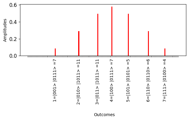
Using the Controlled Weighted Sum pattern Controlled Weighted Sum, where as described in Equation 18, and as described in Equation 24, , and we obtain the result
| (26) |
 |
 |
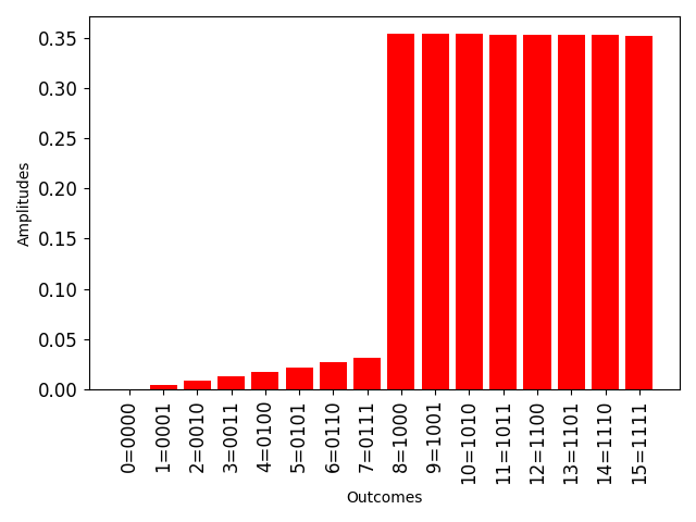
figureTop: Visualization of the amplitudes of a quantum system after applying the operator , using 3 qubits for the key register and and 4 qubits for the value register. The key and value pairs on the x-axis show the result of encoding the binary polynomial in Eq. 25. The distribution of weights applied to the key register (as in Eq. 18) is an approximation of a normal distribution in the amplitudes. Bottom: Visualization of amplitudes of a quantum system, using 3 qubits for the key register and 4 qubits for the value register, after applying the operator and Hadamard gates on the key register. Encoding the linear function in the value register (as in Eq . 24) results in the identity function implemented in amplitudes, repeated for each key value.
Running the quantum computation in a simulator yields (the amplitude of ), and from Equation 26 we obtain . A direct classical calculation gives .
The results of performing this experiment on real quantum hardware can be found in Section 6.
5.2 Payoff Computation in Option Pricing
For simplicity we will use the same discrete function in Section 5.1 to represent a payoff function in an option pricing calculation, whose values are listed below.
Assume that the strike price is , and the price distribution is represented by the values . Then we are interested in computing
We can do that by using the Controlled Weighted Sum pattern Controlled Weighted Sum with hashes
Alternatively, we can encode the function instead of and choose hashes that are identity for non-negative inputs and for negative ones. Note that the hash function acts as a value selector and replaces the comparator used in [10].
5.3 Value at Risk
Within the context and with the notations of the Weighted Sum pattern Weighted Sum, for a given , if and
then we can compute
This allows the computation of Value at Risk when the values represent a price distribution by using a binary search over as also described in [8].
 \captionof
figureVisualization of the amplitudes of a three-qubit quantile quantum state, used in computing Value at Risk for and .
Note that the Controlled Weighted Sum pattern Controlled Weighted Sum can also be used to estimate Value at Risk.
5.4 The Expected Value of a Non-Linear Function
Next, we consider the computation of the expected value of a non-linear function with a normally distributed argument.
Given an integer and , assume we want to compute the weighted sum of a function defined by , for integers , where , :
for weights for , where is the rational function defined by
The rational function is an example of a function that can be used in derivative pricing.
Using the Weighted Sum pattern Weighted Sum, where , as described in Equation 18, for qubits, and encodes normalized values of the function , and , we obtain the result
The states prepared by operators and are shown in Fig. 5.4.
 |
 |
figureTop: Visualization of the amplitudes of a four-qubit quantum state prepared by the unitary operator , as described in Eq. 18. Bottom: Visualization of the amplitudes of a four-qubit quantum state prepared by the unitary operator , which encodes normalized values of the function as described in Section 5.4.
Running the computation in a simulator yields , leading to . A direct classical calculation gives .
5.5 The Expected Value of Linear Functions: Exact Version
5.5.1 Any Linear Function
Next, we consider the computation of the expected value of the identity function, with a normally distributed argument.
Given an integer and , assume we want to compute the weighted sum of a function defined by for integers :
for weights for .
Using the Weighted Sum pattern Weighted Sum, where as described in Equation 18, for qubits, as described in Equation 24, and , we obtain
The states prepared by operators and are shown in Fig. 5.5.1.


As an example, for and , running the computation in a simulator gives , leading to . A direct computation shows that .
5.5.2 A Canonical Linear Function
Given an integer and , assume we want to compute the weighted sum of the identity function defined by for integers :
for weights for .
Using the Weighted Sum pattern Weighted Sum, where as described in Equation 18, for qubits, as described in Equation 24, , and , we obtain
The states prepared by operators and are shown in Fig. 5.5.2.
Running the computation in a simulator gives , leading to .
Note that this canonical implementation of a linear functions allows for the computation of the expected value of any other linear function. For example, we can compute the weighted sum of the values of the function defined by for integers :
for weights for .
For , and therefore , we obtain .
5.6 The Expected Value of Linear Functions: Approximate Version
This section is inspired by the method used in [10], except the approximation is done using amplitudes instead of probabilities.
As in Section 5.5, for a given an integer and , assume we want to compute the weighted sum of the identity function defined by for integers :
for weights for .
We will rely on the canonical approximation from Section 4.3.
Using the Weighted Sum pattern Weighted Sum, where , as described in Equation 18, and , as described in Equation 23, for and a value . Then , , and we obtain
The states prepared by operators and are shown in Fig. 5.6. The circuit will have -qubits to encode the input and an ancillary qubit needed as target for the rotations in the operator .
@*=<0em>@C=2em @R=2em
*!R!<.5em,0em>=<0em>
|
q
⟩
_0 @- [0,-1] *+<1em,.9em> [0,0]="i",[0,0].[2,0]="e",!C *A,"e"+UR;"e"+UL **;"e"+DL **;"e"+DR **;"e"+UR **,"i" @- [0,-1] *+<1em,.9em> [0,0]="i",[0,0].[3,0]="e",!C *B^†,"e"+UR;"e"+UL **;"e"+DL **;"e"+DR **;"e"+UR **,"i" @- [0,-1] @- [0,-1]
*!R!<.5em,0em>=<0em>0 ⋮
*!R!<.5em,0em>=<0em>
|
q
⟩
_n-1 @- [0,-1] *+<1em,.9em> @- [0,-1] *+<1em,.9em> @- [0,-1] @- [0,-1]
*!R!<.5em,0em>=<0em>
|
a
⟩
_0 @- [0,-1] @- [0,-1] *+<1em,.9em> @- [0,-1] @- [0,-1]
 |
 |
figureTop: Visualization of the amplitudes of a three-qubit quantum state prepared by the unitary operator , as described in Eq. 18. Bottom: Visualization of the amplitudes of a three-qubit quantum state prepared by the unitary operator , as described in Eq . 23, with a ancillary qubit added to the circuit to serve as the target for rotations.
As an example, for , and , when running the quantum circuit in a simulator we measure the amplitude of as (it depends only on the distribution), leading to the approximation:
Like in Section 5.5.2, we can use this canonical implementation to compute the expected value of any other linear function, e.g. defined by for integers :
A direct computation shows that
Using the canonical computation above and the fact that from Equation 20 we obtain .
5.7 Value Counting Using Generalized Inner Product

Given integers and , and , weights for , hashes
for integers , and a function for and a value , we want the number of inputs such that .
Therefore, we are interested in calculating the weighted sum of weighted/hashed function values:
Note that we are using the binary representation of keys, i.e. .
Let be an operator that prepares the state , with for , and let be an operator that prepares the state , with for , and let be an operator that encodes the function .
Using the Controlled Weighted Sum pattern Controlled Weighted Sum, we can compute the weighted sum:
Running the computation in a simulator yields the value of (i.e. the amplitude of ) as , and therefore:
so the polynomial has zeros.
The quantum circuit that implements this computation as described above is shown in Fig. 9.
6 Experiments on Quantum Hardware
The experiments discussed in this section were run on IBM quantum devices powered by IBM Quantum Falcon Processors. For each experiment we include the best result of at least 10 runs.
As an experimental observation, we noticed a close correlation between the readout error on a quantum device and the error in inner product computations that does not generally apply to other computations. This may be an interesting area of research.
Expected value of discrete functions.
In this experiment we performed the expected value computation discussed in Section 5.1 on the IBM ibmq_casablanca 7-qubit device with quantum volume 32. Each run of the experiment was performed with 8192 shots.
The amplitude of in the best experiment result was , compared to the simulated value , as calculated in Section 5.1. The readout assignment error at the time of the experiment was 1.93%.
Expected value of linear functions for a trigonometric distribution.
In this experiment we performed the expected value computation discussed in Section 5.5.2 on the IBM ibmq_jakarta 7-qubit device with quantum volume 16. Each run of the experiment was performed with 8192 shots.
The amplitude of in the best experiment result was , compared to the simulated value , as calculated in Section 5.5.2. A comparison between the outcome probability distributions of the experiment and a simulation is shown in Fig. 6. The readout assignment error at the time of the experiment was 4.07%.
 |
 |
figureVisualization of the outcome probabilities of a three-qubit quantum state after performing the computation described in Section 5.5.2, running on ibmq_jakarta (top), and in a simulation environment (bottom). The outcomes different from are grayed out because they do not contribute to the computation result.
Expected value of linear functions for a normal distribution.
In this experiment, we consider the computation of the expected value of the identity function with a normally distributed argument. Using the Weighted Sum pattern Weighted Sum, where is the unitary operator that encodes a normal distribution, as in Appendix B.2, and as described in Equation 24, for qubits. The experiment was performed on the IBM ibmq_jakarta 7-qubit device with quantum volume 16. Each run of the experiment was performed with 8192 shots.
The amplitude of in the best experiment result was , compared to the simulated value . The readout assignment error at the time of the experiment was 2.79%.
7 Related Work
Buhrman et al. [11] define a quantum inner product algorithm, the SWAP test, which efficiently solves the quantum states equality problem with high probability. This algorithm has been used as a building block in several clustering algorithms for supervised and unsupervised machine learning [12].
In the field of quantum deep learning, Tacchino et al. propose an inner product algorithm for implementing quantum neurons [13].
Woerner et al. propose using quantum algorithms for Monte Carlo simulations for financial risk management [8]. These algorithms effectively calculate the inner product of a quantum states representing the distribution of risk factors and asset values.
A widely used class of supervised learning algorithms is Support Vector Machines (SVMs) [14]. Their key computational component is a kernel function that calculates the inner product of feature vectors. This can be implemented by using a feature space implemented as a highly dimensional Hilbert space and a quantum inner product kernel function [15].
8 Concluding Remarks
Efficient methods for calculating expected values, variance, value at risk, etc. are very important in the financial industry.
Such methods rely on computing weighted sums. Finding quantum solutions in this space is an active area of research.
Most notably, the Woerner-Egger method addresses this family of computations by using -rotations to perform multiplication of amplitudes and measurement based addition for implementing weighted sums. In particular, the implementation of the expected value of a canonical linear function allows the calculation of the expected value of any linear function.
The Generalized Inner Product method introduced in this paper allows the calculation of the expected value of any discrete function, not necessarily linear, based on the encoding of a canonical linear function.
It also provides a canonical way to implement input function selection, and thus calculating value at risk (VaR), and a canonical way to implement output value selection, which enables straightforward implementations of comparators needed in option pricing [8, 10], and in general concentration metrics like counting the number of negative values a function takes, or the number of zeros of a function.
The paper provides additional building blocks like exact and approximate encodings for common statistical distributions (e.g. the raised cosine and normal distributions) and functions (e.g. linear functions). Examples of using exact or approximate encoding, and simple or generalized inner product are also included in the paper.
Even stronger generalizations of quantum inner products can be obtained by replacing unitary operators and in Equation 13 with more general operators. This is an interesting future research area.
Acknowledgements.
The authors want to thank Vitaliy Dorum for helping with the development of this manuscript.The views expressed in this article are those of the authors and do not represent the views of Wells Fargo. This article is for informational purposes only. Nothing contained in this article should be construed as investment advice. Wells Fargo makes no express or implied warranties and expressly disclaims all legal, tax, and accounting implications related to this article.
We acknowledge the use of IBM Quantum services for this work. The views expressed are those of the authors, and do not reflect the official policy or position of IBM or the IBM Quantum team.
References
- Grover [1996] Lov K Grover. A fast quantum mechanical algorithm for database search. In Proceedings of the twenty-eighth annual ACM symposium on Theory of computing, pages 212–219, 1996.
- Coppersmith [1994] Don Coppersmith. An approximate fourier transform useful in quantum factoring. Technical Report IBM Research Report RC19642, IBM, 1994.
- Gilliam et al. [2021a] Austin Gilliam, Charlene Venci, Sreraman Muralidharan, Vitaliy Dorum, Eric May, Rajesh Narasimhan, and Constantin Gonciulea. Foundational patterns for efficient quantum computing, 2021a. URL https://arxiv.org/abs/1907.11513.
- Gilliam et al. [2021b] Austin Gilliam, Stefan Woerner, and Constantin Gonciulea. Grover adaptive search for constrained polynomial binary optimization. Quantum, 5:428, Apr 2021b. ISSN 2521-327X. doi: 10.22331/q-2021-04-08-428. URL http://dx.doi.org/10.22331/q-2021-04-08-428.
- IBM [2021] IBM Quantum, 2021. URL https://quantum-computing.ibm.com/.
- O’Donnell [2021] Ryan O’Donnell. Analysis of boolean functions. CoRR, abs/2105.10386, 2021. URL https://arxiv.org/abs/2105.10386.
- Herbert [2021] Steven Herbert. No quantum speedup with grover-rudolph state preparation for quantum monte carlo integration. Physical Review E, 103(6), Jun 2021. ISSN 2470-0053. doi: 10.1103/physreve.103.063302. URL http://dx.doi.org/10.1103/PhysRevE.103.063302.
- Woerner and Egger [2019] Stefan Woerner and Daniel J. Egger. Quantum risk analysis. npj Quantum Information, 5(1), Feb 2019. ISSN 2056-6387. doi: 10.1038/s41534-019-0130-6. URL http://dx.doi.org/10.1038/s41534-019-0130-6.
- Raab and Green [1961] David H Raab and Edward H Green. A cosine approximation to the normal distribution. Psychometrika, 26(4):447–450, 1961. ISSN 0033-3123.
- Stamatopoulos et al. [2020] Nikitas Stamatopoulos, Daniel J. Egger, Yue Sun, Christa Zoufal, Raban Iten, Ning Shen, and Stefan Woerner. Option pricing using quantum computers. Quantum, 4:291, Jul 2020. ISSN 2521-327X. doi: 10.22331/q-2020-07-06-291. URL http://dx.doi.org/10.22331/q-2020-07-06-291.
- Buhrman et al. [2001] Harry Buhrman, Richard Cleve, John Watrous, and Ronald de Wolf. Quantum fingerprinting. Physical Review Letters, 87(16), Sep 2001. ISSN 1079-7114. doi: 10.1103/physrevlett.87.167902. URL http://dx.doi.org/10.1103/PhysRevLett.87.167902.
- Lloyd et al. [2013] Seth Lloyd, Masoud Mohseni, and Patrick Rebentrost. Quantum algorithms for supervised and unsupervised machine learning, 2013.
- Tacchino et al. [2019] Francesco Tacchino, Chiara Macchiavello, Dario Gerace, and Daniele Bajoni. An artificial neuron implemented on an actual quantum processor. npj Quantum Information, 5(1), Mar 2019. ISSN 2056-6387. doi: 10.1038/s41534-019-0140-4. URL http://dx.doi.org/10.1038/s41534-019-0140-4.
- Liu et al. [2020] Yunchao Liu, Srinivasan Arunachalam, and Kristan Temme. A rigorous and robust quantum speed-up in supervised machine learning. CoRR, abs/2010.02174, 2020. URL http://dblp.uni-trier.de/db/journals/corr/corr2010.html#abs-2010-02174.
- Schuld and Killoran [2019] Maria Schuld and Nathan Killoran. Quantum machine learning in feature hilbert spaces. Physical Review Letters, 122(4), Feb 2019. ISSN 1079-7114. doi: 10.1103/physrevlett.122.040504. URL http://dx.doi.org/10.1103/PhysRevLett.122.040504.
Appendix A The Woerner-Egger Approximation Method
Sum of Products.
Given an integer and , probabilities defined for integers , with , and a function we are interested in calculating the sum of products
Solution Sketch.
We paraphrase [8] in this description. We can use the approximation
Then for a constant we have
The products for can be encoded as amplitudes of a quantum states using single-qubit quantum gates acting on an ancillary qubit as described in [8]. In essence, given a quantum state that encodes the probability distribution
the following quantum state can be built by adding an ancillary qubit and applying (controlled) gates to it
where .
The probability of measuring in the ancillary qubit is
and it can be approximated using amplitude estimation algorithms.Then
∎
Note that the summation is done at the probability level, through measurement, not in amplitudes.
The particular case of linear functions is treated in [10] where it is also pointed out that considering only the canonical linear function is sufficient.
Note that:
Adding up the probabilities for outcomes with the ancillary qubit measured as , we get:
Therefore
This can be used to calculate for any linear function by using its intercept and slope. Alternatively, as in [10], we can use the fact that a linear function is completely determined by its minimum and maximum, to obtain
for a linear function .

Intuitively, around half (between and ) of each original amplitude is moved to the corresponding one that measures in the ancilla.
Appendix B Heuristic Circuit Catalog
B.1 Encoding of the Identity Function
The following heuristic circuits provide implementations of a linear function, as discussed in Section 4.4.


|
figureLeft: The quantum circuit that encodes the quantum state using qubits, as defined in Eq . 24. Right: Visualization of the amplitudes of the quantum state with qubits, prepared using the circuit in the figure.


|
figureLeft: The quantum circuit that encodes the quantum state using qubits, as defined in Eq . 24. Right: Visualization of the amplitudes of a quantum state with qubits, prepared using the circuit in the figure.


|
figureLeft: The quantum circuit that encodes the quantum state using qubits, as defined in Eq . 24. Right: Visualization of the amplitudes of a quantum state with qubits, prepared using the circuit in the figure.
B.2 Encoding a Normal Distribution
The following heuristic circuits encode a normal distribution in a quantum state with three or four qubits, respectively.


|
figureLeft: The quantum circuit that encodes a normal distribution in a quantum state with three qubits. Right: Visualization of the amplitudes of a three-quantum state prepared using the circuit in the figure.


|
figureLeft: The quantum circuit that encodes a normal distribution in a quantum state with four qubits. Right: Visualization of the amplitudes of a four-quantum state prepared using the circuit in the figure.