Gluon condensates and effective gluon mass

Color condensates Wetterich 1999; Wetterich 2001c; Wetterich 2001a; Gies et al. 2007 could render the gluons massive through a dynamical realisation of the Higgs mechanism. Note that, strictly speaking, a local gauge symmetry cannot be broken spontaneously. Nonetheless, as is well-known from the description of the electroweak sector of the Standard Model, the language of spontaneous symmetry breaking in a fixed gauge can be particularly useful, and will be employed in what follows.

Below we discuss a color condensate operator, derived from $F_{\mu\nu}$ in the case of the physical gauge group $SU(3)$. Generally, a possible condensate operator of dimension four is given by the traceless hermitian $N_{c}\times N_{c}$ matrices

$\displaystyle\chi^{AB}=\left(F^{AC}_{\mu\nu}F^{CB}_{\mu\nu}-\frac{1}{N_{c}}F^{CD}_{\mu\nu}F^{DC}_{\mu\nu}\delta^{AB}\right)\,,$

(4)

where $A,B,C,D=1,...,N_{c}$ are color indices in the fundamental representation, $F_{\mu\nu}^{AB}=F_{\mu\nu}^{a}(t^{a})^{AB}$. The subtraction of the diagonal term makes the operator traceless, $\chi^{AA}=0$, and for $N_{c}=3$ this is an octet operator. In terms of the field strength components $F^{a}_{\mu\nu}$, the condensate in eq. 4 reads,

$\displaystyle\chi^{AB}=\frac{1}{2}F_{\mu\nu}^{a}F_{\mu\nu}^{b}\Bigl(\{t^{a}\,,\,t^{b}\}^{AB}-\frac{1}{N_{c}}\delta^{ab}\delta^{AB}\Bigr)\,,$

(5)

We note in passing that the above operator is only present for $N_{c}\geq 3$. It vanishes in $SU(2)$, as the symmetric group invariant vanishes, $d^{abc}={\text{tr}}\,t^{a}\{t^{b}\,,\,t^{c}\}=0$. This already suggests that in a realistic condensation scenario leading to a gluon mass gap, eq. 4 should be augmented with further color condensate operators.

Introducing the composite color condensate field $\chi^{AB}$, the quantum effective action $\Gamma$ will contain an induced kinetic term,

$\displaystyle\Gamma_{\chi}=Z_{\chi}\int_{x}(D_{\mu}\chi)^{AB}\,(D_{\mu}\chi)^{BA}\,,$

(6)

with a wave function renormalisation $Z_{\chi}$. For a non-zero expectation value $\langle\chi^{AB}\rangle$, this induces a mass term for some of the gluons,

$\displaystyle m_{A}^{2}\propto Z_{\chi}g_{s}^{2}\langle\chi\rangle^{2}\,.$

(7)

Mass terms for all gluons in $SU(3)$ require condensates of more than one octet in different directions since at least a $U(1)\times U(1)$-subgroup remains unbroken, as for example in Wetterich 1999; Wetterich 2001c; Wetterich 2001a; Gies et al. 2007. This argument also applies to higher gauge groups, $N_{c}\geq 3$, and we have already pointed out in this context that the color condensate operator eq. 5 vanishes for $N_{c}=2$. Besides different mass terms, octet condensates can also induce different effective gauge couplings for different gluons, due to terms in the effective action, see e.g. Hill 1984; Shafi and Wetterich 1984,

$\displaystyle\int_{x}F^{AB}_{\mu\nu}\chi^{BC}F^{CA}_{\mu\nu}\,.$

(8)

This closes our discussion of color condensation in Yang-Mills theories.

The flow equation approach with dynamical composite fields such as the color condensate field discussed in the last section is well understood. It has been introduced and discussed in Ellwanger and Wetterich 1994; Gies and Wetterich 2002; Pawlowski 2007; Lamprecht 2007; Floerchinger and Wetterich 2009; Isaule et al. 2018; Fu et al. 2020; Baldazzi et al. 2021; Daviet and Dupuis 2021; Wegner 1974, for applications to QCD see Gies and Wetterich 2004; Braun 2009; Braun et al. 2016; Rennecke 2015; Cyrol et al. 2018; Fu et al. 2020 and the review Dupuis et al. 2021. However, full computations including the composite field $\chi^{AB}$ require a substantial effort, and will be considered elsewhere.

In the present work we restrict ourselves to a qualitative study, whose principal aim is to gather insights on the possible r$\hat{\textrm{o}}$le of non-singlet condensates in the confining dynamics. This is done by building on results for the condensation of the field strength tensor within functional renormalisation group investigations in Reuter and Wetterich 1994a; Reuter and Wetterich 1997; Eichhorn et al. 2011. Such a colored expectation value of $F_{\mu\nu}$ is linked to non-vanishing expectation values of the color condensate operator $\chi$ in eq. 4 as well as potential non-vanishing expectation values of further color condensate operators. Hence, $\langle F_{\mu\nu}\rangle$ can be used to describe the dynamical emergence of the effective gluon mass via color condensates, for details see Section II.3.

We emphasise that a description in terms of $F_{\mu\nu}$ and its expectation value makes it difficult to include the full dynamics of the color condensate sector as well as the condensation pattern, as this requires the computation of the dynamics of higher order terms in $F_{\mu\nu}$ and covariant derivatives. We also note that such an expansion about $\langle F_{\mu\nu}\rangle$ works naturally for observables or more generally, expectation values of gauge invariant operators. There, singling out a color direction is simply a means of computation. In turn, for gauge-variant expressions the expansion about a non-trivial configuration mixes with the gauge fixing, and it is difficult to undo the color selection quantitatively. Still, it can be done with an additional color averaging $\langle\cdot\rangle_{\textrm{av}}$, which can be implemented systematically. As this concerns the understanding and underlying structure of our work, we further explain this with two simple examples. While important, it is not in our main line of reasoning and hence is deferred to Appendix A.

Note, that such an averaging is to date always implied in lattice simulations of gauge fixed correlation functions as well as in most computations in functional QCD using an expansion about the only color-symmetric background, $\langle F_{\mu\nu}\rangle=0$. The intricacies mentioned above only occur for a quantitative implementation in an expansion about a colored background. It is the current lack of a quantitatively reliable averaging procedure, that causes the current investigation to be of qualitative nature, and constitutes our largest source of systematic error.

In the present work, we compute the respective gauge invariant effective potential ${\cal W}_{\textrm{eff}}(F_{\mu\nu})$ for constant field strength $F_{\mu\nu}$ from the effective action $\Gamma[A]$,

$\displaystyle{\cal W}_{\textrm{eff}}(F_{\mu\nu})=\frac{1}{\cal V}\Gamma_{k}[A(F_{\mu\nu})]\,,$

(9)

with the space time volume ${\cal V}$.

Specifically, we choose gauge fields with the following constant self-dual field strengths: the components $F_{\mu\nu}=0$ for $\mu\nu\neq 01,10,23,32$ vanish, and we have

	$\displaystyle F_{01}=F_{23}=\frac{F^{a}}{2g_{s}}t^{a}\,,\quad F_{01}^{a}=\frac{F^{a}}{2g_{s}}\,,\quad F^{a}=Fn^{a}\,,$		(10a)
with a constant vector $n^{a}$ with $n^{a}n^{a}=1$. The field strength eq. 10a can be generated from the gauge fields
	$\displaystyle A^{a}_{\mu}=-\frac{1}{2}F^{a}_{\mu\nu}x_{\nu}\,.$		(10b)
Evidently, the configuration is self-dual,
	$\displaystyle F_{\mu\nu}=\tilde{F}_{\mu\nu}\,,\quad\textrm{with}\quad\tilde{F}_{\mu\nu}=\frac{1}{2}\epsilon_{\mu\nu\rho\sigma}F_{\rho\sigma}\,,$		(10c)

and is covariantly constant, $[D_{\rho}\,,\,F_{\mu\nu}]=0$.

The classical action and the classical potential ${\cal W}_{\textrm{cl}}$ as well as the color condensate eq. 4 is obtained from the field strength squared, which reads for the configuration eq. 10,

$\displaystyle F_{\mu\nu}F_{\mu\nu}=\frac{F^{2}}{g_{s}^{2}}(n^{a}t^{a})^{2}\,,\qquad F^{a}_{\mu\nu}F^{a}_{\mu\nu}=\frac{1}{g_{s}^{2}}F^{2}\,.$

(11)

For example, for the configuration eq. 10 with eq. 11, the classical potential reduces to

$\displaystyle{\cal W}_{\textrm{cl}}(F^{a})=\frac{1}{2}\,{\text{tr}}\,F^{a}F^{b}\,t^{a}t^{b}=\frac{1}{4g_{s}^{2}}F^{2}\,,$

(12)

where tr is the group trace in the fundamental representation as in eq. 1. From now on we only consider configurations of the type eq. 10, and hence ${\cal W}_{\textrm{eff}}$ will be written as a function of $Fn^{a}$, that is ${\cal W}_{\textrm{eff}}(F^{a})$ instead of ${\cal W}_{\textrm{eff}}(F_{\mu\nu})$. The factor $1/g_{s}^{2}$ in eq. 11 reflects the RG-scaling of the field strength, and has been introduced for convenience. Moreover, as both the gauge fields and the field strength in eq. 10b point in direction $n^{a}$ of the algebra, they can be rotated into the Cartan subalgebra without loss of generality.

Below, we briefly discuss $SU(2)$ and $SU(3)$ gauge groups, the former case as the simplest example, the latter case for its physical relevance:

In the $SU(2)$ gauge group, the Cartan subalgebra is generated by $t^{3}=\sigma^{3}/2$ and the self-dual field strength eq. 10 is given by

$\displaystyle F_{01}=F_{23}=\frac{F}{2g_{s}}\,t^{3}\,.$

(13)

We have already discussed above that in $SU(2)$ the symmetric group invariant $d^{abc}$ vanishes, and hence $\chi^{AB}_{SU(2)}=0$, implying $(F_{\mu\nu}F_{\mu\nu})^{AB}=F_{\mu\nu}^{a}F_{\mu\nu}^{a}\delta^{AB}/4$ for all configurations. For eq. 13 we find

$\displaystyle(F_{\mu\nu}F_{\mu\nu})^{AB}=\frac{F^{2}}{4g_{s}^{2}}\delta^{AB}\,.$

(14)

The explicit computation in this work is done for the physical gauge group $SU(3)$ with the Cartan generators $t^{3},t^{8}$. These are related to the Gell-Mann matrices by $t^{a}=\lambda^{a}/2$, the respective vector $n$ has the components $n^{a}=0$ for $a\neq 3,8$. A self-dual field strength eq. 10 is given by

$\displaystyle F_{01}=F_{23}=\frac{F}{2g_{s}}\big(n^{3}t^{3}+n^{8}t^{8}\big)\,.$

(15)

The octet condensate operator eq. 4 for the configuration eq. 15 reads

	$\displaystyle\chi^{AB}=$	$\displaystyle\,\frac{F^{2}}{2g_{s}^{2}}\Bigl[n^{a}n^{b}\,\{t^{a}\,,\,t^{b}\}^{AB}-\frac{1}{3}\delta^{AB}\Bigr]$
	$\displaystyle=$	$\displaystyle\,\frac{F^{2}}{2g_{s}^{2}}\delta^{AB}\left[\delta^{A1}\nu_{+}+\delta^{A2}\nu_{-}+\delta^{A3}\nu_{3}\right]\,,$		(16)

where

$\displaystyle\nu_{\pm}=\frac{1}{2}\left(\frac{n^{8}}{\sqrt{3}}\pm n^{3}\right)^{2}-\frac{1}{3}\,,\qquad\nu_{3}=\frac{2}{3}(n^{8})^{2}-\frac{1}{3}\,.$

(17)

where the trace(less) condition, $\chi^{AA}=0$, translates into $\nu_{+}+\nu_{-}+\nu_{3}=0$ with $(n^{3})^{2}+(n^{8})^{2}=1$.

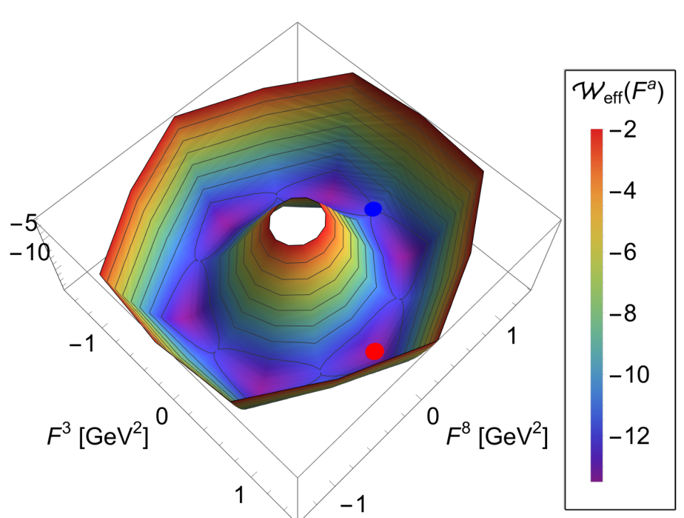
Non-vanishing octet condensate expectation values are in one to one correspondence to non-trivial expectation values of its corresponding gauge-invariant eigenvalues. Hence, a non-trivial expectation value of the field strength triggers one for the octet condensate $\chi^{AB}$ and other color condensate operators. Therefore, in Section IV, we compute the effective potential for covariantly constant field strength or rather ${\cal W}_{\textrm{eff}}[Fn^{a}]$ for the field strength amplitude $Fn^{a}$ defined in eq. 10a, and the constant algebra element $n^{a}t^{a}$ is rotated into the Cartan subalgebra leading to eq. 15. The respective effective potential is shown in Figure 1 for the physical $SU(3)$ case with the two Cartan components $F_{01}n^{3}$ and $F_{01}n^{8}$.

Our explicit computation of the effective gluon mass is based on an expansion about the minimum $\langle F\rangle(n^{a})$ in the three-direction with $n^{a}=\delta^{a3}$. In $SU(2)$ this is the Cartan direction, and in $SU(3)$ one of the absolute minima points in the three-direction, see Figure 1. Then, the expansion about the minimum reads

$\displaystyle F^{a}_{01}=F^{a}_{23}=\frac{\langle F\rangle}{2g_{s}}\delta^{a3}+{\cal O}(a)\,,$

(18)

for both gauge groups, where $a_{\mu}$ is the gauge field, that carries the fluctuations about the field strength expectation value. With eq. 10b we can deduce a gauge field, that generates eq. 18. We find,

$\displaystyle A_{\mu}^{a}=\frac{\langle F\rangle}{4g_{s}}\Bigl(x_{0}\delta_{\mu 1}-x_{1}\delta_{\mu 0}+x_{2}\delta_{\mu 3}-x_{3}\delta_{\mu 2}\Bigr)+a_{\mu}\,,$

(19)

which points in the same Cartan direction as the fields strength. The fluctuation field $a_{\mu}$ carries the dynamics of the gauge field, leading to the ${\cal O}(a)$-terms in eq. 18. Within this setting we shall derive our estimates for the effective gluon mass as well as discuss constraints and bounds for this mass.

It is left to discuss the emergence of an effective gluon mass term in the presence of gluon condensates via the expectation value $\langle F^{a}_{\mu\nu}\rangle\propto\delta^{a3}$ in Equation 18, or any other algebra direction. This expectation value is computed from the effective potential ${\cal W}(F^{a})$ introduced in section II.2.

Expanding the effective potential in powers of the fluctuation field gauge field $a_{\mu}$ leads to contributions to the $n$-point functions of the gauge field, including the two-point function. However, neither a contribution to the mass operator $a_{\mu}^{a}a_{\mu}^{a}$ is generated, nor do we obtain mass terms in specific algebra directions. In particular, no mass contribution in the Cartan $a=3$ direction is induced, as is readily shown for $SU(2)$.

While the effective potential does not contribute to the effective mass term, the latter receives contributions from other terms in the full, gauge invariant quantum effective action $\Gamma[A]$. Such an action can be defined within the background field approach, which will be detailed in Section III. For the time being we simply assume its existence and consider the higher order term

$\displaystyle\Gamma_{F}[A]=\frac{Z_{F}}{4}\int_{x}\,(D_{\mu}F_{\nu\rho})^{a}(D_{\mu}F_{\nu\rho})^{a}\,,$

(20)

where $Z_{F}$ is the wave function renormalisation of the condensate term. Equation 20 is the lowest order term that generates an effective gluon mass term within an expansion about the condensate $\langle F\rangle$. An obvious generalisation of eq. 20 is provided by

$\displaystyle\frac{1}{4}\int_{x}\,(D_{\mu}F_{\rho\sigma})^{a}{Z_{F}}^{ab}_{\rho\sigma\alpha\beta}(F_{\mu\nu})(D_{\mu}F_{\alpha\beta})^{b}\,,$

(21)

with ${Z_{F}}^{ab}_{\rho\sigma\alpha\beta}(0)=Z_{F}\delta_{\rho\alpha}\delta_{\sigma\beta}\delta^{ab}$. In the following we will use the approximation

$\displaystyle{Z_{F}}^{ab}_{\rho\sigma\alpha\beta}(\langle F_{\mu\nu}\rangle)\approx{Z_{F}}^{ab}_{\rho\sigma\alpha\beta}(0)\,,$

(22)

hence only considering the term eq. 20.

Equation 20 leads to an effective gluon mass, but does not contribute to (covariantly constant) solutions of the equations of motions as its first field derivative vanishes for covariantly constant field strengths. The relevant contribution to the effective gluon mass term is obtained by expanding eq. 20 in powers of the gauge field, while treating the field strength within the expansion eq. 18. To that end we conveniently recast eq. 20 into the form

$\displaystyle\Gamma_{F}[A]=-\frac{Z_{F}}{2}\int_{x}\,F_{\nu\rho}^{CB}(D^{2})^{BA}F_{\nu\rho}^{AC}\,,$

(23)

where the factor $1/2$ in eq. 20 is now carried by the trace in the fundamental representation. The ${\cal O}(A^{2})$ term is given by

$\displaystyle\Gamma_{F}[A]=\frac{Z_{F}}{2}\,g_{s}^{2}\int_{x}\,(F_{\nu\rho}F_{\nu\rho})^{AB}\,(A_{\mu}A_{\mu})^{BA}+\cdots\,,$

(24)

and we expand $(F_{\nu\rho}F_{\nu\rho})^{AB}$ about the field strength expectation value eq. 18. This implies a non-vanishing condensate expectation value for eq. 4 as well as non-vanishing values for other color condensate operators. The expansion about eq. 18 leads us to

$\displaystyle(F_{\nu\rho}F_{\nu\rho})^{AB}=\frac{1}{g_{s}^{2}}\langle F\rangle^{2}[(n^{a}t^{a})^{2}]^{AB}+{\cal O}(A)\,.$

(25)

We drop the higher order terms in eq. 25 and insert it in eq. 24, to wit,

$\displaystyle\Gamma_{F}[A]\simeq\frac{Z_{F}}{2}\langle F\rangle^{2}\int_{x}\,{\text{tr}}\,(t^{3})^{2}A_{\mu}^{2}+\cdots\,,$

(26)

with the group trace in the fundamental representation. Now we evaluate eq. 26 for the configurations eq. 10, which leads to our final expression for the effective gluon mass triggered by an expectation value of the field strength proportional to $t^{3}$. For general gauge groups, eq. 26 is not color blind, which originates in the colored expansion point. It can be used to deduce the color blind mass by a color average discussed in Appendix A.

Before we come to our final color blind estimates, we exemplify eq. 26 within $SU(2)$ and $SU(3)$. We first discuss the simple example of an $SU(2)$ gauge group. There, the configuration eq. 18 leads to an $F_{\mu\nu}^{2}$ that is proportional to the identity tensor $\mathbbm{1}$ in the algebra, as $4(t^{3})^{2}=\mathbbm{1}$. Indeed, as discussed below eq. 13, general field strength tensors lead to diagonal $F_{\mu\nu}^{2}$. In summary, in $SU(2)$, a field strength condensate in the $t^{3}$-direction leads to

$\displaystyle\Gamma_{F}[A]\simeq\frac{1}{2}m_{3}^{2}\int_{x}A^{a}_{\mu}A_{\mu}^{a}+\cdots\,,\quad m_{3}^{2}=\frac{Z_{F}}{8}\langle F\rangle^{2}\,,$

(27)

with a uniform mass $m_{3}$ for all gluons. The subscript indicates that, while uniform, the mass is generated by $\langle F^{a}_{\mu\nu}\rangle\propto\delta^{a3}$. Importantly, eq. 27 entails that a color condensate leads to gluons with an effective mass. However, the current procedure with an expansion about a non-vanishing field strength does not allow to directly infer the full effective gluon mass obtained in a color blind computation from $m_{3}^{2}$ in eq. 27. At this state we only can offer estimates, whose derivation is deferred to the end of the present section.

Before we come to these estimates, we proceed with the $SU(3)$ example. There, we also use the Cartan-valued configuration eq. 18 (with $n^{8}=0$) as one of the absolute minima in the full effective potential ${\cal W}_{\textrm{eff}}$ points in this direction, see Figure 1. In contradistinction to $SU(2)$, the square $4(t^{3})^{2}$ is not the identity matrix in the algebra, but a projection onto the first two colors,

$\displaystyle[(t^{3})^{2}]^{AB}=\frac{1}{4}\delta^{AB}\Bigl(\delta^{A1}+\delta^{A2}\Bigr)\,.$

(28)

As expected, the expansion about a minimum of the field strength, related to one about the octet condensate eq. 4, breaks color, and indeed, the gluon with the third color is massless if only considering contributions from $\Gamma_{F}$. Hence, while the present expansion shows, that the gluons acquire an effective mass term $\propto\delta^{ab}$, the relation of its necessarily color blind strength $m_{A}^{2}$ to the color-sensitive masses derived here is not straightforward.

Therefore, in the present work we simply deduce self-consistency constraints for the effective mass $m_{A}^{2}$ starting with the gluon mass $m_{3}^{2}$, inferred from a field strength in the $t^{3}$ direction. To begin with, color symmetry can be restored by averaging over global color rotations as always implied in lattice simulations as well as in most computations in functional QCD. After this averaging, all masses are identical and non-vanishing. A color average of eq. 26 leads us to

$\displaystyle\Gamma_{A^{2}}[A]=\frac{Z_{F}}{2}f_{\textrm{av}}(N_{c})\langle F\rangle^{2}\int_{x}\,A^{a}_{\mu}A_{\mu}^{a}\,,$

(29)

with $f_{\textrm{av}}(N_{c})$ encodes the color average of the factor $(t^{3})^{2}$ in eq. 26,

$\displaystyle f_{\textrm{av}}(N_{c})=\langle(t^{3})^{2}\rangle_{\textrm{av}}\,.$

(30)

The color average in eq. 30 necessarily leads to a color insensitive sum over all generators squared in the fundamental representation, which is simply the second Casimir $C_{2}(N_{c})=(N_{c}^{2}-1)/(2N_{c})$ times the identity matrix. Moreover, there is an undetermined prefactor $c_{\textrm{av}}(N_{c})$, which leads us to

$\displaystyle\hskip-0.42677pt\Bigl\langle(t^{3})^{2}\Bigr\rangle_{\textrm{av}}=c_{\textrm{av}}(N_{c})\sum_{a=1}^{N_{c}^{2}-1}(t^{a})^{2}=c_{\textrm{av}}(N_{c})C_{2}(N_{c})\mathbbm{1}\,.$

(31)

In the present work we will only provide constraints for $c_{\textrm{av}}(N_{c})$ and hence for $f_{\textrm{av}}(N_{c})$ in eq. 30. For example, a ’natural’ bound for the averaging factor is unity, $c_{\textrm{av}}(N_{c})\leq 1$.

In summary we arrive at

$\displaystyle m^{2}_{A}=\frac{Z_{F}}{2}\,f_{\textrm{av}}(N_{c})\,\langle F\rangle^{2}\,,$

(32)

In Section III.3 we will show, that self-consistency of the averaging in the large $N_{c}$ limit entails that in this limit $f_{\textrm{av}}(N_{c})\propto N_{c}$. Indeed, this limit holds true for $N_{c}$-independent $c_{\textrm{av}}$. In particular this includes the case, where we saturate the ’natural’ bound $c_{\textrm{av}}=1$, leading to

$\displaystyle f_{\textrm{av}}=(N_{c}^{2}-1)/(2N_{c})\,.$

(33)

For this saturation $f_{\textrm{av}}$ we obtain

$\displaystyle m^{2}_{A}=\frac{Z_{F}}{4}\,\frac{N_{c}^{2}-1}{N_{c}}\,\langle F\rangle^{2}\,,$

(34)

Equation 34 will eventually yield our estimate of the effective gluon mass. In Section III, we present the formalism employed for working with the constant field strength configurations in eq. 11. The computation of the minimum position $F^{a}=\langle F\rangle\,n^{a}$ is detailed in Section IV, and an estimate of the wave function of the condensate together with the result for the mass gap is presented in Section V.

The gauge invariance of the background field effective action allows us to embed the momentum-dependent kinetic terms and vertices in an expansion about a vanishing gauge field in full gauge invariant terms that reduce to the original ones for $A_{\mu}\to 0$. An important example is given by the (transverse) kinetic term of the gauge field, see e.g. Braun et al. 2010; Eichhorn et al. 2011; Fister and Pawlowski 2013,

$\displaystyle\Gamma[A]\propto\frac{1}{2}\int_{p}A^{a}_{\mu}(p)\,Z_{A}(p^{2})\,p^{2}\,\Pi_{\mu\nu}^{\bot}(p)\,A^{a}_{\nu}(-p)\,,$

(37)

with the abbreviation $\int_{p}=\int d^{4}p/(2\pi)^{4}$, and the transverse and longitudinal projection operators

$\displaystyle\Pi_{\mu\nu}^{\bot}(p)=\delta_{\mu\nu}-\frac{p_{\mu}p_{\nu}}{p^{2}}\,,\qquad\Pi_{\mu\nu}^{\parallel}(p)=\frac{p_{\mu}p_{\nu}}{p^{2}}\,.$

(38)

The kinetic operator $Z_{A}(p^{2})p^{2}$ is identified as the $A_{\mu}\to 0$ limit of the second field derivative of a gauge invariant term in the effective action $\Gamma[A]$. This leads us straightforwardly to the parametrisation

	$\displaystyle\Gamma[A]=\frac{1}{2}\int{\text{tr}}F_{\mu\nu}f_{A,\mu\nu\rho\sigma}(D)F_{\rho\sigma}+\cdots\,,$			(39a)
with the split
	$\displaystyle f_{A,\mu\nu\rho\sigma}(D)=$	$\displaystyle\,\frac{1}{2}Z_{A}(\Delta_{s})(\delta_{\mu\rho}\delta_{\nu\sigma}-\delta_{\mu\sigma}\delta_{\nu\rho})$
		$\displaystyle+F_{\gamma\delta}f_{A,\gamma\delta\mu\nu\rho\sigma}(D)\,.$		(39b)
In eq. 39b, we have introduced the spin-$s$ Laplacians
	$\displaystyle\Delta_{0}=-D^{2}\,,\qquad\Delta_{1,\mu\nu}={\cal D}_{T,\mu\nu}=-D^{2}\delta_{\mu\nu}+2ig_{s}\,F_{\mu\nu}\,,$			(39c)

see also eq. 86. Equation 39b represents the most general parametrisation for a covariant function coupled to two field strengths. Since $f_{A,\gamma\delta\mu\nu\rho\sigma}$ is a function of the Laplacian $D$, higher order terms in the field strength tensor are contained in the second term of eq. 39b. For $A_{\mu}=0$, all these decompositions reduce to their the momentum-dependent versions. In particular, the kinetic term eq. 37 is obtained from eq. 39b by taking two gauge field derivatives at $A=0$.

A further relevant example is the sum of the classical action and the term $\Gamma_{F}$ in eq. 20 that generates the effective gluon mass. This combination is obtained with

$\displaystyle Z_{A}(-D^{2})=Z_{A}-Z_{F}D^{2}\,,\quad f_{A,\gamma\delta\mu\nu\rho\sigma}=0\,.$

(40)

Here, $Z_{A}$ is the constant background wave function renormalisation multiplying the classical action, which also entails $Z_{A}=Z_{g_{s}}^{-2}$.

The example given in eq. 40 is central for two reasons: Firstly, it demonstrates how the condensate studied in this work emerges from the general, gauge-invariant form of the effective action eq. 39a, which is defined in the next section within the background field formalism. Secondly, it establishes a link between the wave function renormalisation of the condensate and the kinetic operator of the gluon field $Z_{A}(\Delta_{s})$. More explicitly, due to the generality of the split eq. 39b, eq. 40 entails that the wave function renormalisation of the condensate eq. 20 is simply given by the $D^{2}$-coefficient of the dressing function of the gluon propagator. In the limit of vanishing background, this simply corresponds to the $p^{4}$-term in the inverse gluon propagator.

Note that the use of different $\Delta_{s}$ in the split eq. 39b leads to different forms for $f_{\mu_{1}\cdots\mu_{6}}$, thus modifying the parametrisation of the kinetic term. Still, the different field modes carry different spin, and the use of the respective Laplacians makes the split in eq. 39b to be the most natural. Typically, higher order terms within this split are suppressed in the effective action. For example, the second derivative of the classical Yang-Mills action with respect to the gauge field is given by $\Delta_{1}={\cal D}_{T}$, multiplied by a covariant transverse projection operator. For covariantly constant fields with $[D,F]=0$, we get

$\displaystyle\frac{\delta^{2}}{\delta A_{\rho}\delta A_{\sigma}}\frac{1}{2}\int_{x}{\text{tr}}F_{\mu\nu}^{2}={\cal D}_{T,\rho\gamma}\,\Pi_{\gamma\sigma}^{\bot}(D)\,,$

(41)

where the trace is taken in the fundamental representation. Above, we introduced the covariant transverse and longitudinal projections,

$\displaystyle\Pi_{\mu\nu}^{\bot}(D)=\delta_{\mu\nu}-\Pi_{\mu\nu}^{\parallel}(D)\,,\quad\Pi_{\mu\nu}^{\parallel}(D)=D_{\mu}\frac{1}{D^{2}}D_{\nu}\,.$

(42)

Equation 42 defines a decomposition in a covariantly transverse subspace with $D_{\mu}\Pi^{\bot}(D)=0$. It is complete, $\Pi^{\bot}(D)+\Pi^{\parallel}(D)=\mathbbm{1}$, and trivially orthogonal. Finally, the operators have the projection property $(\Pi^{\bot}(D))^{2}=\Pi^{\bot}(D)$ and $(\Pi^{\parallel}(D))^{2}=\Pi^{\parallel}(D)$.

When supplemented by a wave function renormalisation $Z_{A}({\cal D}_{T})$, eq. 41 provides a very good approximation of the full two-point function of the background gluon. This suggests the split in eq. 39b with the spin one Laplacian $\Delta_{1}={\cal D}_{T}$ for the transverse two-point function, and with the second term being subleading,

	$\displaystyle\Gamma_{AA,\mu\nu}^{(2,0)}[A,0]=$	$\displaystyle\,Z_{A}(\mathcal{D}_{T})\,\mathcal{D}_{T,\mu\sigma}\,\Pi_{\sigma\nu}^{\bot}(D)$
		$\displaystyle\,+F_{\gamma\delta}\,\Delta f_{A,\gamma\delta\mu\sigma}(D)\,\Pi_{\sigma\nu}^{\bot}(D)\,,$		(43)

where $\Delta f_{A,\gamma\delta\mu\nu}$ is a combination of derivatives of $f_{A,\mu\nu\rho\sigma}$ fully contracted with powers of the field strength, see eq. 39b, and $\bar{A}=A$. The transversality of eq. 43 follows from the gauge invariance of the background field effective action, as does its covariance. In eq. 43 we have used the notation

$\displaystyle\Gamma_{\bar{A}^{n}\phi_{i_{1}}\cdots\phi_{i_{m}}}^{(n,m)}[\bar{A},\phi]=\frac{\Gamma[\bar{A},\phi]}{\delta\bar{A}^{n}\delta\phi^{m}}\,,\qquad\phi=(a,c,\bar{c})\,,$

(44)

with $\phi$ denoting the ghost and gluon fluctuation field. We shall use the split eq. 39b leading to eq. 43 and similar natural splits for the covariant versions of the momentum dependent two-point functions, thus going from the Landau gauge to the Landau-DeWitt gauge.

In particular one finds, that a similar line of arguments holds true for the kinetic operator $Z_{a}(p^{2})p^{2}$ of the fluctuation field $a_{\mu}$,

$\displaystyle\Gamma_{aa,\mu\nu}^{(0,2)}[0,0]=Z_{a}(p^{2})\,p^{2}\Pi_{\mu\nu}^{\bot}(p)+\frac{1}{\xi}p^{2}\Pi_{\mu\nu}^{\parallel}(p)\,,$

(45)

where eq. 38 was employed, and a diagonal form in the algebra, $\mathbbm{1}^{ab}=\delta^{ab}$, is implied. Background gauge invariance entails that $\Gamma^{(0,2)}[A,0]$ is a covariant operator under the background gauge transformations eq. 35. In consequence, the transverse part of $\Gamma_{aa}^{(0,2)}[A,0]$ can be parametrised by the generic form of a background gauge covariant function already employed in eq. 39b, i.e.,

	$\displaystyle\Gamma_{aa,\mu\nu}^{(0,2)}[A,0]=$	$\displaystyle\,Z_{a}(\mathcal{D}_{T})\,\mathcal{D}_{T,\mu\sigma}\,\Pi_{\sigma\nu}^{\bot}(D)-\frac{1}{\xi}D^{2}\,\Pi_{\mu\nu}^{\parallel}(D)$
		$\displaystyle\,+F_{\gamma\delta}\,\Delta f_{a,\gamma\delta\mu\sigma}(D)\,\Pi_{\sigma\nu}^{\bot}(D)\,.$		(46)

In eq. 46 we have used the spin-1 Laplacian $\Delta_{1}={\cal D}_{T}$ defined in eq. 39c in the wave function renormalisation $Z_{a}$, since the transverse fluctuating gluon is a spin-1 field. For two-flavour QCD, the validity of such covariant expansions has been confirmed explicitly for the quark-gluon vertex, whose non-classical tensor structure can be related to higher order gauge-invariant terms $\bar{q}\not{D}^{n}q$ Cyrol et al. 2018.

Finally, in the case of the ghost two-point function we parametrise

$\displaystyle\Gamma_{c\bar{c}}^{(0,2)}[A,0]=-D^{2}Z_{c}(-D^{2})+F_{\mu\nu}\,\Delta f_{c,\mu\nu}(D)\,,$

(47)

where the use of the spin zero Laplacian in eq. 47 is suggested by the ghost being a spin zero field. For $A_{\mu}=0$, the ghost two point function in eq. 47 reduces to that in standard covariant gauges.

The infrared behaviour of $Z_{a}(p)$ in the Landau gauge is an extensively studied subject, both on the lattice as well as with functional approaches, see e.g. Aguilar et al. 2008; Fischer et al. 2009; Binosi and Papavassiliou 2009; Maas 2013; Huber 2020a; Dupuis et al. 2021. In particular, two types of solutions have emerged:

(i) The scaling solution Kugo and Ojima 1979 has an infrared vanishing gluon propagator and a scaling infrared behaviour,

$\displaystyle Z_{a,\textrm{IR}}\propto(-D^{2})^{-2\kappa}\,,\qquad Z_{c,\textrm{IR}}\propto(-D^{2})^{\kappa}\,.$

(48)

with $\kappa\approx 0.6$. In eq. 48 we have dropped terms proportional to the field strength. Note that in this IR solution the ghost dressing function is infrared divergent. For the present computations we shall use the fRG results from Cyrol et al. 2016 within a quantitatively reliable approximation, for respective DSE results see Huber 2020b.

(ii) An entire family of decoupling or massive solutions Cornwall 1982, where the gluon propagator and the ghost dressing function saturate at finite non-vanishing values at the origin, in agreement with the IR behaviour found in large-volume lattice simulations. Specifically, we have

$\displaystyle Z_{a,\textrm{IR}}\propto$

$\displaystyle\,\frac{1+c_{a}D^{2}\log\left(\frac{-D^{2}}{\Lambda_{\textrm{QCD}}^{2}}\right)}{-D^{2}}\,,\qquad Z_{c,\textrm{IR}}\propto c_{c}\,.$

(49)

Note that the fluctuating propagator can be mapped to the background one by means of an exact identity, characteristic of the Batalin-Vilkoviski formalism, which involves a special two-point function, see e.g. Binosi and Papavassiliou 2002; Binosi and Papavassiliou 2009.

We emphasise that both types of solutions agree quantitatively for momenta $p^{2}\gtrsim\Lambda_{\textrm{QCD}}^{2}$, with $\Lambda_{\textrm{QCD}}$ related to the infrared mass gap. As a result, the deviations induced to phenomenological observables by the use of either type are quantitatively minimal, see e.g. Cyrol et al. 2018; Gao et al. 2021. In fact, in the present work we will cover all potential solutions listed above, and show that their IR differences are immaterial to the central question of the presence of dynamical condensate formation.

Both types of solutions, eq. 48 and eq. 49, are infrared irregular, and do not admit a Taylor expansion about $-D^{2}=0$. Instead, we can expand the wave function renormalisations about the infrared asymptotics. Making use of the relation between the condensate and gluon wave function renormalisation established in eq. 40, we arrive at

	$\displaystyle Z_{a/A}(-D^{2})=$	$\displaystyle\,Z_{a/A,\textrm{IR}}(-D^{2})+(-D^{2})\,Z_{a/A,F}$
		$\displaystyle\,+\mathcal{O}(D^{4})\,,$		(50)

for both $Z_{a}$ and $Z_{A}$ with $Z_{a/A,\textrm{IR}}$ defined in eq. 48 and eq. 49, and $Z_{a/A,F}$ is the wave function $Z_{F}$ for fluctuation and background field respectively. The first term $Z_{a/A,\textrm{IR}}$ carries the irregular infrared asymptotic behaviour, and $Z_{a/A,F}$ is the (uniquely defined) constant prefactor of the linear term in $-D^{2}$. The expansion section III.2 makes explicit that scaling and decoupling solutions only differ in the IR leading term $Z_{a/A,\textrm{IR}}$, while coinciding in the expansion in powers of $-D^{2}$. This in particular entails that the overlap between gluon propagator and the condensate eq. 20 is independent of the leading IR behaviour of the respective solution, scaling or decoupling.

We are ultimately interested in the physical mass gap $m_{\mathrm{gap}}$ of the fluctuation field $a_{\mu}$ resulting from the condensate term eq. 20 in the full field $A=\bar{A}+a$. The derivation of the fluctuation field mass gap works analogously to that of eq. 32 in Section II.3, and leads to a contribution $\Gamma_{\textrm{gap}}$ in the effective action with

$\displaystyle\Gamma_{\textrm{gap}}=\frac{1}{2}m_{\textrm{gap}}^{2}\int_{x}a^{b}_{\mu}a^{b}_{\mu}\,,$

(51)

where the effective gluon mass of the fluctuation gluon $a_{\mu}$ is given by

$$m^{2}_{\mathrm{gap}}=\frac{Z_{\mathrm{cond}}}{2}f_{\textrm{av}}(N_{c})\langle F\rangle^{2}\,.$$

(52)

with $Z_{\textrm{cond}}=Z_{a,F}$ and the averaging factor $f_{\textrm{av}}(N_{c})$ introduced in eq. 29 and discussed there. In particular we have $Z_{F}=Z_{A,F}\neq Z_{\mathrm{cond}}$. The wave function $Z_{F}$ is used in eq. 32 for the mass term in a gauge invariant effective action, and in the present approach this is the background field effective action. The difference between the wave functions $Z_{F}$ and $Z_{\mathrm{cond}}$ is the ratio of the respective wave functions of the background and fluctuation gluons.

In eq. 40 we observed that the wave function renormalisation $Z_{\mathrm{cond}}$ of the condensate studied here generally appears in the dressing function of the respective gluon propagator, cf. section III.2. This connection will be utilised in Section V to determine $Z_{\mathrm{cond}}$ from the input gluon propagators Cyrol et al. 2016 employed in the computation of the background field effective potential $\mathcal{W}_{\textrm{eff}}(F^{a})$. Supplemented with the non-trivial effective potential minimum $\langle F\rangle$, this procedure eventually lead to our heuristic estimate of the gluon mass gap in Landau gauge Yang-Mills theory.

The effective gluon masses $m^{2}_{A}$ in eq. 32 and $m_{\textrm{gap}}^{2}$ in eq. 52 show an explicit $1/N_{c}$-scaling, while no $N_{c}$-scaling is present in the large $N_{c}$ limit, if the theory is formulated in the ’t Hooft coupling

$\displaystyle\lambda=N_{c}g_{s}^{2}\,.$

(53)

This property serves as a self-consistency check of our computation and specifically our group average used to derive eq. 32, eq. 52 and entailed in $f_{\textrm{av}}(N_{c})$

An illustrative and relevant example are the functional relations of the two-point function $\Gamma_{aa}^{(0,2)}(p)$. Cast in a relation for the wave function $Z_{a}(p)$, they read

$\displaystyle Z(p^{2})=Z_{\textrm{in}}+g_{s}^{2}\,N_{c}\,\textrm{Diags}_{1}+{\cal O}(N^{0}_{c})\,,$

(54)

where the right hand side stands for the typical loop diagrams of e.g. (integrated) fRG flows or Dyson-Schwinger equations. Here, $Z_{\textrm{in}}$ stands for the input dressing, either the one at the initial UV cutoff scale (fRG) or the classical dressing (DSE). In most cases the ${\cal O}(N_{c}^{0})$ term is dropped, for an exception as well as a respective discussion see Corell et al. 2018. The term $\textrm{Diags}_{1}$ stands for the loop integral that depends on the wave functions of all the fields and the full vertex dressings. Importantly, the functional relations for all other vertex dressings and wave functions have the same form as eq. 54. Accordingly, if dropping the subleading term of the order $O(N_{c}^{0})$, all functional relations only depend on the ’t Hooft coupling eq. 56, and so do all correlation functions. Respective lattice studies also reveal that the large $N_{c}$-limit is achieved already for $N_{c}\gtrsim 3$ for most correlation functions, for a review see Lucini and Panero 2014.

In summary we deduce, that in the large $N_{c}$-limit the only $N_{c}$-dependence of the effective gluon masses $m^{2}_{A}$ in eq. 32 and $m_{\textrm{gap}}^{2}$ in eq. 52 is implicit in the dependence on the ’t Hooft coupling eq. 56. This concludes our brief discussion of the $N_{c}$-scaling of correlation functions.

The relations for the effective gluon mass, eq. 32, eq. 52, show an even more direct scaling consistency: $Z_{\textrm{F}}$ is an expansion term in the two-point function of the fluctuating gluon. Moreover, in the presence of the condensate this two-point function approaches the effective gluon for vanishing momentum,

$\displaystyle\lim_{p\to 0}\Pi^{\bot}_{\mu\nu}(p)\Gamma_{aa,\mu\nu}^{(0,2)}(p)=3\,m^{2}_{\textrm{gap}}\,.$

(55)

Accordingly, both $Z_{\textrm{cond}}$ and $m_{\textrm{gap}}$ have the same $N_{c}$-scaling (only dependent on the ’t Hooft coupling in the large $N_{c}$-limit) as well as the same RG-scaling. In conclusion, the ratio $Z_{\textrm{cond}}/m^{2}_{\textrm{gap}}$ is manifestly RG-invariant as well as $N_{c}$-independent in the large $N_{c}$-limit. This implies already, that the RG-invariant information in the effective gluon mass is given by $f_{\textrm{av}}(N_{c})\,\langle F\rangle^{2}$. The value of the mass itself depends on the RG-condition and should not be confused with the gluon mass gap. The latter can be defined as the inverse screening length of the gluon propagator which is indeed RG-invariant.

In summary, $f_{\textrm{av}}(N_{c})\,\langle F\rangle^{2}$ should be $N_{c}$-independent in the large $N_{c}$-limit. This fixes the $N_{c}$-scaling of $f_{\textrm{av}}(N_{c})$, given that of $\langle F\rangle^{2}$. The $N_{c}$-scaling of the latter is obtained by an $N_{c}$-analysis of the effective potential, whose explicit computation is detailed in Section IV and Appendix D. Here we only need that it consists out of an ultraviolet classical piece of the form eq. 12 and a term that depends on $N_{c}F^{2}$,

$\displaystyle{\cal W}_{\textrm{eff}}(F^{a})=\frac{1}{4g_{s}^{2}}F^{2}+\Delta{\cal W}_{\textrm{eff}}(N_{c}F^{2})\,,$

(56)

see Section IV.2. In eq. 56, $g_{s}^{2}$ is the strong coupling at a large momentum scale $k_{\textrm{UV}}$, and we will use $k_{\textrm{UV}}=20$ GeV for this scale later on. We now absorb $N_{c}$ into the field strength squared amplitude $F^{2}$, i.e. $\bar{F}^{2}=N_{c}F^{2}$. With eq. 53 this leads us to

$\displaystyle{\cal W}_{\textrm{eff}}(F^{a})=\frac{1}{4\lambda}\bar{F}^{2}+\Delta{\cal W}_{\textrm{eff}}(\bar{F}^{2})\,,$

(57)

and consequently

$\displaystyle\langle\bar{F}\rangle=\bar{F}_{\textrm{min}}(\lambda)\qquad\longrightarrow\qquad\langle F\rangle=\frac{1}{\sqrt{N_{c}}}\bar{F}_{\textrm{min}}(\lambda)\,.$

(58)

The $1/N_{c}$-scaling for $\langle F\rangle^{2}$ derived in eq. 58, is confirmed numerically in Appendix D. There, the effective potential and its minimum is computed in a leading order $N_{c}$ approximation and hence shows the asymptotic $1/N_{c}$ scaling even for $N_{c}=2$. This $N_{c}$-scaling is rooted in the adjoint representation trace of $n^{a}t^{a}$ appearing the definition of the covariantly constant field strength in eq. 10, cf. appendix C. We have confirmed its numerical presence in a comparison of $N_{c}=2,3$.

References

- Fritzsch and Gell-Mann (1972) H. Fritzsch and M. Gell-Mann, eConf C720906V2, 135 (1972), arXiv:hep-ph/0208010 .
- Fritzsch and Minkowski (1975) H. Fritzsch and P. Minkowski, Nuovo Cim. A 30, 393 (1975).
- Michael and Teper (1989) C. Michael and M. Teper, Nucl. Phys. B 314, 347 (1989).
- Bali et al. (1993) G. S. Bali, K. Schilling, A. Hulsebos, A. C. Irving, C. Michael, and P. W. Steph̃enson (UKQCD), Phys. Lett. B 309, 378 (1993), arXiv:hep-lat/9304012 .
- Morningstar and Peardon (1999) C. J. Morningstar and M. J. Peardon, Phys. Rev. D 60, 034509 (1999), arXiv:hep-lat/9901004 .
- Gregory et al. (2012) E. Gregory, A. Irving, B. Lucini, C. McNeile, A. Rago, C. Richards, and E. Rinaldi, JHEP 10, 170 (2012), arXiv:1208.1858 [hep-lat] .
- Athenodorou and Teper (2020) A. Athenodorou and M. Teper, JHEP 11, 172 (2020), arXiv:2007.06422 [hep-lat] .
- Szczepaniak et al. (1996) A. Szczepaniak, E. S. Swanson, C.-R. Ji, and S. R. Cotanch, Phys. Rev. Lett. 76, 2011 (1996), arXiv:hep-ph/9511422 .
- Szczepaniak and Swanson (2003) A. P. Szczepaniak and E. S. Swanson, Phys. Lett. B 577, 61 (2003), arXiv:hep-ph/0308268 .
- Mathieu et al. (2009) V. Mathieu, N. Kochelev, and V. Vento, Int. J. Mod. Phys. E 18, 1 (2009), arXiv:0810.4453 [hep-ph] .
- Dudal et al. (2011) D. Dudal, M. S. Guimaraes, and S. P. Sorella, Phys. Rev. Lett. 106, 062003 (2011), arXiv:1010.3638 [hep-th] .
- Meyers and Swanson (2013) J. Meyers and E. S. Swanson, Phys. Rev. D 87, 036009 (2013), arXiv:1211.4648 [hep-ph] .
- Cloet and Roberts (2014) I. C. Cloet and C. D. Roberts, Prog. Part. Nucl. Phys. 77, 1 (2014), arXiv:1310.2651 [nucl-th] .
- Sanchis-Alepuz et al. (2015) H. Sanchis-Alepuz, C. S. Fischer, C. Kellermann, and L. von Smekal, Phys. Rev. D 92, 034001 (2015), arXiv:1503.06051 [hep-ph] .
- Souza et al. (2020) E. V. Souza, M. Narciso Ferreira, A. C. Aguilar, J. a. Papavassiliou, C. D. Roberts, and S.-S. Xu, Eur. Phys. J. A 56, 25 (2020), arXiv:1909.05875 [nucl-th] .
- Huber et al. (2020) M. Q. Huber, C. S. Fischer, and H. Sanchis-Alepuz, Eur. Phys. J. C 80, 1077 (2020), arXiv:2004.00415 [hep-ph] .
- Cucchieri and Mendes (2007) A. Cucchieri and T. Mendes, PoS LATTICE2007, 297 (2007), arXiv:0710.0412 [hep-lat] .
- Cucchieri and Mendes (2008) A. Cucchieri and T. Mendes, Phys. Rev. Lett. 100, 241601 (2008), arXiv:0712.3517 [hep-lat] .
- Cucchieri and Mendes (2010) A. Cucchieri and T. Mendes, Phys. Rev. D 81, 016005 (2010), arXiv:0904.4033 [hep-lat] .
- Sternbeck et al. (2006) A. Sternbeck, E. M. Ilgenfritz, M. Muller-Preussker, A. Schiller, and I. L. Bogolubsky, PoS LAT2006, 076 (2006), arXiv:hep-lat/0610053 .
- Bogolubsky et al. (2007) I. L. Bogolubsky, E. M. Ilgenfritz, M. Muller-Preussker, and A. Sternbeck, PoS LATTICE2007, 290 (2007), arXiv:0710.1968 [hep-lat] .
- Bogolubsky et al. (2009) I. L. Bogolubsky, E. M. Ilgenfritz, M. Muller-Preussker, and A. Sternbeck, Phys. Lett. B 676, 69 (2009), arXiv:0901.0736 [hep-lat] .
- Oliveira and Silva (2009) O. Oliveira and P. J. Silva, PoS LAT2009, 226 (2009), arXiv:0910.2897 [hep-lat] .
- Pawlowski et al. (2010) J. M. Pawlowski, D. Spielmann, and I.-O. Stamatescu, Nucl. Phys. B 830, 291 (2010), arXiv:0911.4921 [hep-lat] .
- Oliveira and Bicudo (2011) O. Oliveira and P. Bicudo, J. Phys. G 38, 045003 (2011), arXiv:1002.4151 [hep-lat] .
- Maas (2013) A. Maas, Phys. Rept. 524, 203 (2013), arXiv:1106.3942 [hep-ph] .
- Aguilar et al. (2008) A. C. Aguilar, D. Binosi, and J. Papavassiliou, Phys. Rev. D 78, 025010 (2008), arXiv:0802.1870 [hep-ph] .
- Boucaud et al. (2008) P. Boucaud, J.-P. Leroy, A. L. Yaouanc, J. Micheli, O. Pene, and J. Rodriguez-Quintero, JHEP 06, 012 (2008), arXiv:0801.2721 [hep-ph] .
- Fischer et al. (2009) C. S. Fischer, A. Maas, and J. M. Pawlowski, Annals Phys. 324, 2408 (2009), arXiv:0810.1987 [hep-ph] .
- Binosi and Papavassiliou (2009) D. Binosi and J. Papavassiliou, Phys. Rept. 479, 1 (2009), arXiv:0909.2536 [hep-ph] .
- Huber (2020a) M. Q. Huber, Phys. Rept. 879, 1 (2020a), arXiv:1808.05227 [hep-ph] .
- Pawlowski et al. (2004) J. M. Pawlowski, D. F. Litim, S. Nedelko, and L. von Smekal, Phys.Rev.Lett. 93, 152002 (2004), arXiv:hep-th/0312324 [hep-th] .
- Gies (2012) H. Gies, Lect. Notes Phys. 852, 287 (2012), arXiv:hep-ph/0611146 .
- Braun (2012) J. Braun, J. Phys. G 39, 033001 (2012), arXiv:1108.4449 [hep-ph] .
- Dupuis et al. (2021) N. Dupuis, L. Canet, A. Eichhorn, W. Metzner, J. M. Pawlowski, M. Tissier, and N. Wschebor, Phys. Rept. 910, 1 (2021), arXiv:2006.04853 [cond-mat.stat-mech] .
- Braun et al. (2010) J. Braun, H. Gies, and J. M. Pawlowski, Phys.Lett. B684, 262 (2010), arXiv:0708.2413 [hep-th] .
- Fister and Pawlowski (2013) L. Fister and J. M. Pawlowski, Phys. Rev. D 88, 045010 (2013), arXiv:1301.4163 [hep-ph] .
- Farhi and Jackiw (1982) E. Farhi and R. Jackiw, eds., Dyanamical gauge symmetry breaking. A collection of reprints (1982).
- Aitchison and Hey (2013) I. J. R. Aitchison and A. J. G. Hey, Gauge Theories in Particle Physics: A Practical Introduction, Volume 2: Non-Abelian Gauge Theories : QCD and The Electroweak Theory, Fourth Edition (Taylor & Francis, 2013).
- Cornwall (1982) J. M. Cornwall, Phys. Rev. D 26, 1453 (1982).
- Lavelle and Schaden (1988) M. J. Lavelle and M. Schaden, Phys. Lett. B 208, 297 (1988).
- Lavelle (1991) M. Lavelle, Phys. Rev. D 44, 26 (1991).
- Wetterich (2001a) C. Wetterich, (2001a), arXiv:hep-ph/0102248 .
- Wetterich (2001b) C. Wetterich, Phys. Rev. D 64, 036003 (2001b), arXiv:hep-ph/0008150 .
- Wetterich (2004) C. Wetterich, AIP Conf. Proc. 739, 123 (2004), arXiv:hep-ph/0410057 .
- Eichhorn et al. (2011) A. Eichhorn, H. Gies, and J. M. Pawlowski, Phys. Rev. D 83, 045014 (2011), [Erratum: Phys.Rev.D 83, 069903 (2011)], arXiv:1010.2153 [hep-ph] .
- Cyrol et al. (2016) A. K. Cyrol, L. Fister, M. Mitter, J. M. Pawlowski, and N. Strodthoff, Phys. Rev. D 94, 054005 (2016), arXiv:1605.01856 [hep-ph] .
- Wetterich (1999) C. Wetterich, Phys. Lett. B 462, 164 (1999), arXiv:hep-th/9906062 .
- Wetterich (2001c) C. Wetterich, Eur. Phys. J. C 18, 577 (2001c), arXiv:hep-ph/9908514 .
- Gies et al. (2007) H. Gies, J. Jaeckel, J. M. Pawlowski, and C. Wetterich, Eur.Phys.J. C49, 997 (2007), arXiv:hep-ph/0608171 [hep-ph] .
- Hill (1984) C. T. Hill, Phys. Lett. B 135, 47 (1984).
- Shafi and Wetterich (1984) Q. Shafi and C. Wetterich, Phys. Rev. Lett. 52, 875 (1984).
- Ellwanger and Wetterich (1994) U. Ellwanger and C. Wetterich, Nucl. Phys. B 423, 137 (1994), arXiv:hep-ph/9402221 .
- Gies and Wetterich (2002) H. Gies and C. Wetterich, Phys.Rev. D65, 065001 (2002), arXiv:hep-th/0107221 [hep-th] .
- Pawlowski (2007) J. M. Pawlowski, Annals Phys. 322, 2831 (2007), arXiv:hep-th/0512261 [hep-th] .
- Lamprecht (2007) F. Lamprecht, (2007), diploma thesis Heidelberg.
- Floerchinger and Wetterich (2009) S. Floerchinger and C. Wetterich, Phys.Lett. B680, 371 (2009), arXiv:0905.0915 [hep-th] .
- Isaule et al. (2018) F. Isaule, M. C. Birse, and N. R. Walet, Phys. Rev. B 98, 144502 (2018), arXiv:1806.10373 [cond-mat.quant-gas] .
- Fu et al. (2020) W.-j. Fu, J. M. Pawlowski, and F. Rennecke, Phys. Rev. D 101, 054032 (2020), arXiv:1909.02991 [hep-ph] .
- Baldazzi et al. (2021) A. Baldazzi, R. B. A. Zinati, and K. Falls, (2021), arXiv:2105.11482 [hep-th] .
- Daviet and Dupuis (2021) R. Daviet and N. Dupuis, (2021), arXiv:2111.11458 [cond-mat.quant-gas] .
- Wegner (1974) F. J. Wegner, Journal of Physics C: Solid State Physics 7, 2098 (1974).
- Gies and Wetterich (2004) H. Gies and C. Wetterich, Phys.Rev. D69, 025001 (2004), arXiv:hep-th/0209183 [hep-th] .
- Braun (2009) J. Braun, Eur. Phys. J. C64, 459 (2009), arXiv:0810.1727 [hep-ph] .
- Braun et al. (2016) J. Braun, L. Fister, J. M. Pawlowski, and F. Rennecke, Phys. Rev. D94, 034016 (2016), arXiv:1412.1045 [hep-ph] .
- Rennecke (2015) F. Rennecke, Phys. Rev. D92, 076012 (2015), arXiv:1504.03585 [hep-ph] .
- Cyrol et al. (2018) A. K. Cyrol, M. Mitter, J. M. Pawlowski, and N. Strodthoff, Phys. Rev. D97, 054006 (2018), arXiv:1706.06326 [hep-ph] .
- Reuter and Wetterich (1994a) M. Reuter and C. Wetterich, (1994a), arXiv:hep-th/9411227 .
- Reuter and Wetterich (1997) M. Reuter and C. Wetterich, Phys. Rev. D 56, 7893 (1997), arXiv:hep-th/9708051 .
- Abbott (1981) L. F. Abbott, Nucl. Phys. B 185, 189 (1981).
- Kugo and Ojima (1979) T. Kugo and I. Ojima, Prog. Theor. Phys. Suppl. 66, 1 (1979).
- Huber (2020b) M. Q. Huber, Phys. Rev. D 101, 114009 (2020b), arXiv:2003.13703 [hep-ph] .
- Binosi and Papavassiliou (2002) D. Binosi and J. Papavassiliou, Phys. Rev. D 66, 025024 (2002), arXiv:hep-ph/0204128 .
- Gao et al. (2021) F. Gao, J. Papavassiliou, and J. M. Pawlowski, Phys. Rev. D 103, 094013 (2021), arXiv:2102.13053 [hep-ph] .
- Corell et al. (2018) L. Corell, A. K. Cyrol, M. Mitter, J. M. Pawlowski, and N. Strodthoff, SciPost Phys. 5, 066 (2018), arXiv:1803.10092 [hep-ph] .
- Lucini and Panero (2014) B. Lucini and M. Panero, Prog. Part. Nucl. Phys. 75, 1 (2014), arXiv:1309.3638 [hep-th] .
- Litim and Pawlowski (1998) D. F. Litim and J. M. Pawlowski, in Workshop on the Exact Renormalization Group (1998) pp. 168–185, arXiv:hep-th/9901063 .
- Berges et al. (2002) J. Berges, N. Tetradis, and C. Wetterich, Phys. Rept. 363, 223 (2002), arXiv:hep-ph/0005122 .
- Braun et al. (2019) J. Braun, M. Leonhardt, and J. M. Pawlowski, SciPost Phys. 6, 056 (2019), arXiv:1806.04432 [hep-ph] .
- van Baal (2000) P. van Baal, (2000), arXiv:hep-ph/0008206 .
- Herbst et al. (2015) T. K. Herbst, J. Luecker, and J. M. Pawlowski, (2015), arXiv:1510.03830 [hep-ph] .
- Narison (2009) S. Narison, Phys. Lett. B 673, 30 (2009), arXiv:0901.3823 [hep-ph] .
- Bali and Pineda (2016) G. S. Bali and A. Pineda, AIP Conf. Proc. 1701, 030010 (2016), arXiv:1502.00086 [hep-ph] .
- Boucaud et al. (2018) P. Boucaud, F. De Soto, K. Raya, J. Rodríguez-Quintero, and S. Zafeiropoulos, Phys. Rev. D 98, 114515 (2018), arXiv:1809.05776 [hep-ph] .
- Aguilar et al. (2021a) A. C. Aguilar, C. O. Ambrósio, F. De Soto, M. N. Ferreira, B. M. Oliveira, J. Papavassiliou, and J. Rodríguez-Quintero, Phys. Rev. D 104, 054028 (2021a), arXiv:2107.00768 [hep-ph] .
- Parisi and Petronzio (1980) G. Parisi and R. Petronzio, Phys. Lett. B 94, 51 (1980).
- Bernard (1982) C. W. Bernard, Phys. Lett. B 108, 431 (1982).
- Bernard (1983) C. W. Bernard, Nucl. Phys. B 219, 341 (1983).
- Donoghue (1984) J. F. Donoghue, Phys. Rev. D 29, 2559 (1984).
- Mandula and Ogilvie (1987) J. E. Mandula and M. Ogilvie, Phys. Lett. B 185, 127 (1987).
- Ji and Amiri (1990) C.-R. Ji and F. Amiri, Phys. Rev. D 42, 3764 (1990).
- Halzen et al. (1993) F. Halzen, G. I. Krein, and A. A. Natale, Phys. Rev. D 47, 295 (1993).
- Yndurain (1995) F. J. Yndurain, Phys. Lett. B 345, 524 (1995).
- Field (2002) J. H. Field, Phys. Rev. D 66, 013013 (2002), arXiv:hep-ph/0101158 .
- Philipsen (2002) O. Philipsen, Nucl. Phys. B 628, 167 (2002), arXiv:hep-lat/0112047 .
- Luna et al. (2005) E. G. S. Luna, A. F. Martini, M. J. Menon, A. Mihara, and A. A. Natale, Phys. Rev. D 72, 034019 (2005), arXiv:hep-ph/0507057 .
- Deur et al. (2016) A. Deur, S. J. Brodsky, and G. F. de Teramond, Nucl. Phys. 90, 1 (2016), arXiv:1604.08082 [hep-ph] .
- Aguilar et al. (2021b) A. C. Aguilar, M. N. Ferreira, and J. Papavassiliou, (2021b), arXiv:2111.09431 [hep-ph] .
- Braun et al. (2021) J. Braun, Y.-r. Chen, W.-j. Fu, F. Gao, F. Ihssen, A. Geissel, J. Horak, C. Huang, J. M. Pawlowski, F. Rennecke, F. Sattler, B. Schallmo, C. Schneider, Y.-y. Tan, S. Töpfel, R. Wen, J. Wessely, N. Wink, and S. Yin, (2021).
- van Egmond et al. (2021) D. M. van Egmond, U. Reinosa, J. Serreau, and M. Tissier, (2021), arXiv:2104.08974 [hep-ph] .
- Litim (2000) D. F. Litim, Phys. Lett. B 486, 92 (2000), arXiv:hep-th/0005245 .
- Fister and Pawlowski (2015) L. Fister and J. M. Pawlowski, Phys. Rev. D 92, 076009 (2015), arXiv:1504.05166 [hep-ph] .
- Reuter and Wetterich (1994b) M. Reuter and C. Wetterich, Nucl. Phys. B 417, 181 (1994b).
- Gies (2002) H. Gies, Phys. Rev. D 66, 025006 (2002), arXiv:hep-th/0202207 .
- Dunne and Schubert (2002) G. V. Dunne and C. Schubert, JHEP 08, 053 (2002), arXiv:hep-th/0205004 .
- Mitter et al. (2015) M. Mitter, J. M. Pawlowski, and N. Strodthoff, Phys.Rev. D91, 054035 (2015), arXiv:1411.7978 [hep-ph] .
- (107) J. M. Pawlowski, C. S. Schneider, and N. Wink, .
- Pawlowski et al. (2021) J. M. Pawlowski, C. S. Schneider, and N. Wink, (2021), arXiv:2102.01410 [hep-ph] .
- Aguilar et al. (2012) A. C. Aguilar, D. Ibanez, V. Mathieu, and J. Papavassiliou, Phys. Rev. D 85, 014018 (2012), arXiv:1110.2633 [hep-ph] .
- Binosi et al. (2012) D. Binosi, D. Ibanez, and J. Papavassiliou, Phys. Rev. D 86, 085033 (2012), arXiv:1208.1451 [hep-ph] .
- Aguilar et al. (2018) A. C. Aguilar, D. Binosi, C. T. Figueiredo, and J. Papavassiliou, Eur. Phys. J. C 78, 181 (2018), arXiv:1712.06926 [hep-ph] .
- Eichmann et al. (2021) G. Eichmann, J. M. Pawlowski, and J. a. M. Silva, Phys. Rev. D 104, 114016 (2021), arXiv:2107.05352 [hep-ph] .
- Schwinger (1962a) J. S. Schwinger, Phys. Rev. 125, 397 (1962a).
- Schwinger (1962b) J. S. Schwinger, Phys. Rev. 128, 2425 (1962b).
- Jackiw and Johnson (1973) R. Jackiw and K. Johnson, Phys. Rev. D 8, 2386 (1973).
- Eichten and Feinberg (1974) E. Eichten and F. Feinberg, Phys. Rev. D 10, 3254 (1974).
- Aguilar et al. (2014) A. C. Aguilar, D. Binosi, D. Ibañez, and J. Papavassiliou, Phys. Rev. D 89, 085008 (2014), arXiv:1312.1212 [hep-ph] .
- Aguilar et al. (2016) A. C. Aguilar, D. Binosi, C. T. Figueiredo, and J. Papavassiliou, Phys. Rev. D 94, 045002 (2016), arXiv:1604.08456 [hep-ph] .