On Nonlocal Cohesive Continuum Mechanics and Cohesive Peridynamic Modeling (CPDM) of Inelastic Fracture Journal: arXiv

Jing Han ^† Shaofan Li ^‡ Note: Email:shaofan@berkeley.edu Haicheng Yu ^§ Jun Li ^⋆ A-man Zhang ^† Address: ^†College Of Shipbuilding Engineering, Harbin Engineering University, Harbin, Heilongjiang, 150001, China,
^‡ Department of Civil and Environmental Engineering, University of California, Berkeley,
California, 94720, USA;
^§ College of Naval Architecture and Ocean Engineering, Dalian Maritime University, Dalian, Liaoning, 116026, China;
^⋆ College of Science, Wuhan University of Technology, Wuhan, Hubei, 430070, China.

Abstract

In this work, we developed a bond-based cohesive peridynamics model (CPDM) and apply it to simulate inelastic fracture by using the meso-scale Xu-Needleman cohesive potential [1]. By doing so, we have successfully developed a bond-based cohesive continuum mechanics model with intrinsic stress/strain measures as well as consistent and built-in macro-scale constitutive relations. The main novelties of this work are:
(1) We have shown that the cohesive stress of the proposed nonlocal cohesive continuum mechanics model is exactly the same as the nonlocal peridynamic stress;
(2) For the first time, we have applied an irreversible built-in cohesive stress-strain relation in a bond-based cohesive peridynamics to model inelastic material behaviors without prescribing phenomenological plasticity stress-strain relations;
(3) The cohesive bond force possesses both axial and tangential components, and they contribute a nonlinear constitutive relation with variable Poisson’s ratios;
(4) The bond-based cohesive constitutive model is consistent with the cohesive fracture criterion, and
(5) We have shown that the proposed method is able to model inelastic fracture and simulate ductile fracture of small scale yielding in the nonlocal cohesive continua.

Several numerical examples have been presented to be compared with the finite element based continuum cohesive zone model, which shows that the proposed approach is a simple, efficient and effective method to model inelastic fracture in the nonlocal cohesive media.

Keywords:

Bond-based peridynamics; Cohesive zone model; Crack growth; Inelastic fracture; Nonlocal continuum mechanics; Poisson’s ratio;

1 Introduction

Peridynamics [2, 3, 4, 5, 6] was originally proposed as a nonlocal reformulation of continuum mechanics aiming at modeling fracture and damage in solids. Peridynamics research has been an active research field in computational mechanics, especially in numerical simulation of fracture and failure in materials and structures [7, 8]. The non-local peridynamics theory is formulated with an integral form of equation of motion, which replaces the partial differential form of equation of motion in conventional continuum mechanics of local form. By doing so, it is applicable to a much broader class of displacement fields that allow discontinuities and singularities, thus providing much needed physical modeling of many non-local media such as cementitious concrete materials, soil and rocks, ice and snow, and many other granular materials.

In spite of its success, the original bond-based peridynamics has some major limitations: (1) It has been difficult to evaluate peridynamic stress in the bond-based peridynamics; (2) Its main applications have been limited to model brittle fracture or crack growth in macro-scale linear elastic solids with restrictions on certain material constants such as Poisson’s ratio; (3) It needs a semi-empirical parameter, namely the critical bond stretch, $s_{0}$ , to set up the onset of fracture or crack growth criterion, and (4) It has difficulty modeling material or structure fracture with continuum mechanical stress and strain measures of finite deformation, even though peridynamics is intrinsically formulated under the setting of continuum mechanical finite deformation.

The main cause for these limitations is that the current formulation of the bond-based peridynamics has not reached to a status to be a truly bond-based nonlocal continuum mechanics, and these inadequacies are reflected by lacking of stress measures, corresponding macro-scale constitutive models, as well as damage models or fracture criteria. For example, Cauchy’s relation is an intrinsic limitation for the bond-based peridynamics for a fixed Poisson’s ratio [9]. Moreover, the peridynamic stress formulated by Lehoucq and Silling [10, 4] is cumbersome to use so that it has been rarely adopted in computations, which leads to the lack of consistent macro-scale constitutive relations in the bond-based peridynamics. In particular, the bond-based peridynamics almost does not have an universally consistent inelastic constitutive relation at macro-scale.

To address all these fundamental issues in the bond-based peridynamics, in this work, we developed a bond-based cohesive peridynamic (CPDM) model for nonlocal continua by utilizing the meso-scale Xu-Needleman cohesive potential. In this paper, we shall demonstrate that by combing the classical cohesive zone model [11]. The cohesive zone peridynamics has been studied by several authors, e.g. [12, 13, 14], however, the focus of the present work is not on cohesive zone peridynamics, but a general bond-based peridynamics that utilizes the mesoscale cohesive potential to model a nonlocal continuum. From this perspective, we are developing a novel nonlocal continuum mechanics modeling.

The paper is organized into six sections. In Section 2, we first lay out the kinematics of nonlocal continuum. Then, in Section 3, we present the formal theory of cohesive nonlocal continuum. One highlight of this work is the presentation of cohesive stress formulation, which is elaborated in Section 4. Several numerical examples, both two-dimensional (2D) and three-dimensional (3D), are presented in Section 5, to validate and verify the proposed CPDM theory and formulation. We summarize the work in Section 6 with a few remarks.

2 Nonlocal continuum kinematics

To establish a bond-based peridynamics model for cohesive continua, we first describe the material bond kinematics. Given the referential and the current configurations $\mathcal{B}_{0}$ and $\mathcal{B}_{t}$ , for any pair of peridynamic particles $({\bf X},{\bf X}^{\prime})$ that interact with each other, the bond vector is described by $\boldsymbol{\xi}$ and $\boldsymbol{\eta}$ as follows,

\boldsymbol{\xi}=\boldsymbol{X}^{\prime}-\boldsymbol{X};~~\boldsymbol{\eta}=\boldsymbol{u}(\boldsymbol{X}^{\prime},t)-\boldsymbol{u}(\boldsymbol{X},t),~{\rm and}~~\boldsymbol{\zeta}={\bf x}^{\prime}-{\bf x}~,

(1)

where ${\bf X}$ is the marker of the material point in the referential configuration $\mathcal{B}_{0}$ , while ${\bf x}$ is the coordinate of the same material point in the current $\mathcal{B}_{t}$ . In Eq. (1), ${\bf u}({\bf X},t)$ is the displacement of the material point ${\bf X}$ .The schematic diagram is demonstrated in Fig. 1.

Refer to caption — Figure 1: Kinematics of material points

Following the kinematic relation and notation of continuum mechanics, we have

{\bf x}={\bf X}+{\bf u}~\to~\boldsymbol{\zeta}=\boldsymbol{\xi}+\boldsymbol{\eta}~.

(2)

where $\boldsymbol{\xi}$ describes the original bond vector, $\boldsymbol{\zeta}$ describes the deformed bond vector, or the bond vector in the current configuration, while $\boldsymbol{\eta}$ is the deformation of the bond vector.

We first define the first type nonlocal material gradient for a vector function ${\bf G}({\bf X})$ at the point ${\bf X}$ as

\widetilde{\nabla}_{X}\otimes[{\bf G}({\bf X})]:=\Bigl[\int_{\mathcal{H}_{X}}w(\xi)\Delta{\bf G}\otimes({\bf K}^{-1}{\mbox{\boldmath$\xi$}})dV_{{\bf X}^{\prime}}\Bigr]

(3)

where $\widetilde{\nabla}_{X}$ denotes the nonlocal differential operator in the referential configuration. For more detailed discussions on nonlocal differential operators, the readers are referred to [15, 16]. The integration domain in Eq.(3), $\mathcal{H}_{X}$ , is called as a horizon that is centered at ${\bf X}$ , and ${\mbox{\boldmath$\xi$}}={\bf X}^{\prime}-{\bf X}$ , $\xi=|{\mbox{\boldmath$\xi$}}|$ where ${\bf X}^{\prime},{\bf X}\in\mathcal{H}_{X}$ . In the integrand of Eq.(3), $\Delta{\bf G}:={\bf G}(\bf X^{\prime})-{\bf G}(\bf X)$ , and $w(\xi)$ is a window function or weight function, which satisfies the condition

\int_{\mathcal{H}_{X}}w(\xi)dV_{{\bf X}^{\prime}}=1~.

In practice, it is often chosen as the Gaussian distribution function or the cubic spline function. The linear transformation ${\bf K}:={\bf K}({\bf X})$ is the shape tensor or the moment matrix at the material point ${\bf X}$ that is defined as

{\bf K}({\bf X}):=\int_{\mathcal{H}_{X}}w(\xi){\mbox{\boldmath$\xi$}}\otimes{\mbox{\boldmath$\xi$}}dV_{{\bf X}^{\prime}}~.

(4)

In actual computations, the nonlocal gradient of an arbitrary vector function ${\bf G}({\bf X})$ may be calculated based on the following formula,

\widetilde{\nabla}_{X}\otimes[{\bf G}({\bf X}_{I})]=\Bigl[\sum_{J=1,J\not=I}^{N_{I}}w(X_{IJ})\Delta{\bf G}_{IJ}\otimes({\bf X}_{IJ}{\bf K}_{I}^{-1})\Delta V_{J}\Bigr]

(5)

where

{\bf K}_{I}={\bf K}({\bf X}_{I})=\sum_{J=1,J\not=I}^{N_{I}}w(X_{IJ}){\bf X}_{IJ}\otimes{\bf X}_{IJ}\Delta V_{J}~.

and $V_{J}$ is the discrete volume associated with the particle $J$ .

For example, we can write the nonlocal deformation gradient in a form as

Then in an abstract form, we may denote the nonlocal gradient operator as a form of a local gradient operator

\widetilde{\nabla}_{{\bf X}}\otimes(\bullet)\Bigm|_{{\bf X}}:=\left[\int_{\mathcal{H}_{X}}w(\xi)\Delta(\bullet)\otimes({\mbox{\boldmath$\xi$}}{\bf K}_{X}^{-1}){\rm d}V_{{\bf X}^{\prime}}\right]

(7)

where the symbol $(\bullet)$ denotes the arbitrary vector field, and $\Delta(\bullet):=(\bullet)^{\prime}-(\bullet)$ . Note that Eq. (7) defines the nonlocal differential operator by using linear function basis. For higher order nonlocal differential operators theory, readers may refer to [17] and [18] and references therein.

3 Nonlocal cohesive continuum model

Following Silling and Lequcq (2008), we have the nonlocal balance of linear momentum as follows,

\rho({\bf X})\ddot{\bf u}({\bf X},t)=\int_{\mathcal{B}}\Bigl({\bf t}^{s}({\bf X}^{\prime},{\bf X},t)-{\bf t}^{s}({\bf X},{\bf X}^{\prime},t)\Bigr)dV_{{\bf X}^{\prime}}+{\bf b}({\bf X},t)

(8)

where $\rho$ is the mass density of the continuum medium; ${\bf b}({\bf X},t)$ is the body force per unit mass, and ${\bf t}^{s}({\bf X}^{\prime},{\bf X},t)$ is called the force state vector, and ${\bf f}({\bf X}^{\prime},{\bf X}):={\bf t}^{s}({\bf X}^{\prime},{\bf X},t)-{\bf t}^{s}({\bf X},{\bf X}^{\prime},t)$ represents the force density acting at the material point ${\bf X}$ by the material point ${\bf X}^{\prime}$ .

As shown by Silling and Lehoucq [4], the force density can be related to the force state vector as

{\bf t}^{s}({\bf X}^{\prime},{\bf X},t)={1\over 2}{\bf f}(\boldsymbol{\eta},\boldsymbol{\xi}),~~{\rm and}~~{\bf t}^{s}({\bf X},{\bf X}^{\prime},t)={1\over 2}{\bf f}(-\boldsymbol{\eta},-\boldsymbol{\xi})~.

(9)

where ${\bf t}^{s}({\bf X}^{\prime},{\bf X})$ is the force state vector that material particle ${\bf X}^{\prime}$ exerts on the material particle ${\bf X}$ , in which the superscript indicates the force state; $V_{X}$ is the volume of the particle ${\bf X}$ depending on the specific discretization, while ${\bf f}(\boldsymbol{\eta},\boldsymbol{\xi})$ is a force density, which is required to be antisymmetric, i.e.

{\bf f}(\boldsymbol{\eta},\boldsymbol{\xi})=-{\bf f}(-\boldsymbol{\eta},-\boldsymbol{\xi})~.

(10)

In the literature, we often express the above property in an equivalent form,

{\bf f}({\bf X}^{\prime},{\bf X})=-{\bf f}({\bf X},{\bf X}^{\prime})~.

(11)

3.1 Meso-scale Xu-Needleman model

To construct the internal force density in a nonlocal cohesive continuum, we adopt the mesoscale cohesive potential as the material bond potential, in contrast with the prototype microelastic brittle (PMB) potential adopted in the original bond based peridynamics, e.g. [2].

In this work, we adopt the mesoscale Xu-Needleman potential [1] as the material bond potential. Unlike atomistic pair bond potential in molecular dynamics, the meso-scale Xu-Needleman potential can generate both axial interaction force as well as tangential interaction force. To construct a pair bond with normal and tangential cohesive bond force components we define

\boldsymbol{\eta}_{n}=(\boldsymbol{\eta}\cdot\boldsymbol{n})\boldsymbol{n}~~{\rm and}~~\boldsymbol{\eta}_{t}=\boldsymbol{\eta}-(\boldsymbol{\eta}\cdot\boldsymbol{n})\boldsymbol{n}

(12)

where

\boldsymbol{n}=\frac{\boldsymbol{\xi}}{\left|\boldsymbol{\xi}\right|}

(13)

in other words

\boldsymbol{\eta}=\boldsymbol{\eta}_{n}+\boldsymbol{\eta}_{t};~~~\boldsymbol{\eta}_{n}\perp\boldsymbol{\eta}_{t};~~\eta=\sqrt{\eta_{n}^{2}+\eta_{t}^{2}}~.

(14)

We consider the following meso-scale Xu-Needleman potential:

where $\phi_{n}$ , $\delta_{n}$ , $\delta_{t}$ , $r$ , and $q$ are coefficients which will later be determined. The dimension of $\phi_{n}$ should be $N/m^{5}$ , $\delta_{n}$ and $\delta_{t}$ are characteristic lengths, $r$ and $q$ are dimensionless. One can see that, the physical implications of the five coefficients are not the same as those in original Xu-Needleman potential. The bond force density that particle $\boldsymbol{X}^{\prime}$ acts on particle $\boldsymbol{X}$ can be obtained as follows:

\boldsymbol{f}=\frac{\partial\phi}{\partial\boldsymbol{\eta}}=\boldsymbol{f}_{n}+\boldsymbol{f}_{t}

(16)

Considering the fact

	$\displaystyle{\frac{\partial}{\partial{\mbox{\boldmath$\eta$}}}}\exp\bigl(-{\frac{{\mbox{\boldmath$\eta$}}\cdot{\bf n}}{\delta_{n}}}\bigr)=-{1\over\delta_{n}}\exp\bigl(-{{\mbox{\boldmath$\eta$}}\cdot{\bf n}\over\delta_{n}}\bigr){\bf n}$
	$\displaystyle{\partial\over\partial{\mbox{\boldmath$\eta$}}}\exp\Bigl(-{1\over\delta_{t}^{2}}\bigm\|{\mbox{\boldmath$\eta$}}-{\mbox{\boldmath$\eta$}}\cdot{\bf n}\bigm\|^{2}\Bigr)=-{2\over\delta_{t}^{2}}\exp\Bigl(-{1\over\delta_{t}^{2}}\bigm\|{\mbox{\boldmath$\eta$}}-{\mbox{\boldmath$\eta$}}\cdot{\bf n}\bigm\|^{2}\Bigr)\Bigl({\mbox{\boldmath$\eta$}}-({\mbox{\boldmath$\eta$}}\cdot{\bf n}){\bf n}\Bigr)$

we then have

$\displaystyle\boldsymbol{f}(\boldsymbol{X},\boldsymbol{X}^{\prime})$	$\displaystyle=$	$\displaystyle-\frac{\phi_{n}}{\delta_{n}}\exp{(-\frac{\boldsymbol{\eta}\cdot\boldsymbol{n}}{\delta_{n}})}\{[(-r+\frac{\boldsymbol{\eta}\cdot\boldsymbol{n}}{\delta_{n}})\frac{1-q}{r-1}$	(17)
	$\displaystyle-$	$\displaystyle[q+(\frac{r-q}{r-1})\frac{\boldsymbol{\eta}\cdot\boldsymbol{n}}{\delta_{n}}]\exp(-\frac{1}{\delta_{t}^{2}}\left\|\boldsymbol{\eta}-(\boldsymbol{\eta}\cdot\boldsymbol{n})\boldsymbol{n}\right\|^{2})$
	$\displaystyle+$	$\displaystyle(\frac{r-q}{r-1})\exp(-\frac{1}{\delta_{t}^{2}}\left\|\boldsymbol{\eta}-(\boldsymbol{\eta}\cdot\boldsymbol{n})\boldsymbol{n}\right\|^{2})]\boldsymbol{n}$
	$\displaystyle-$	$\displaystyle[\frac{2\delta_{n}}{\delta_{t}^{2}}(q+(\frac{r-q}{r-1})\frac{\boldsymbol{\eta}\cdot\boldsymbol{n}}{\delta_{n}})$
	$\displaystyle\cdot$	$\displaystyle\exp(-\frac{1}{\delta_{t}^{2}}\left\|\boldsymbol{\eta}-(\boldsymbol{\eta}\cdot\boldsymbol{n})\boldsymbol{n}\right\|^{2})](\boldsymbol{\eta}-(\boldsymbol{\eta}\cdot\boldsymbol{n})\boldsymbol{n})\}$

It should be reminded that, when deriving $\boldsymbol{f}(\boldsymbol{X},\boldsymbol{X}^{\prime})$ , the local coordinate system established on origin $\boldsymbol{X}$ is adopted; in contrast, the derivation of $\boldsymbol{f}(\boldsymbol{X}^{\prime},\boldsymbol{X})$ is based on the coordinate system whose origin is $\boldsymbol{X}^{\prime}$ . Then the bond force that particle $\boldsymbol{X}$ acts on particle $\boldsymbol{X}^{\prime}$ is as follows:

$\displaystyle\boldsymbol{f}(\boldsymbol{X}^{\prime},\boldsymbol{X})$	$\displaystyle=$	$\displaystyle-\frac{\phi_{n}}{\delta_{n}}\exp{(-\frac{\boldsymbol{\eta}\cdot\boldsymbol{n}}{\delta_{n}})}\{[(-r+\frac{\boldsymbol{\eta}\cdot\boldsymbol{n}}{\delta_{n}})\frac{1-q}{r-1}$	(18)
	$\displaystyle-$	$\displaystyle[q+(\frac{r-q}{r-1})\frac{\boldsymbol{\eta}\cdot\boldsymbol{n}}{\delta_{n}}]\exp(-\frac{1}{\delta_{t}^{2}}\left\|\boldsymbol{\eta}-(\boldsymbol{\eta}\cdot\boldsymbol{n})\boldsymbol{n}\right\|^{2})$
	$\displaystyle+$	$\displaystyle(\frac{r-q}{r-1})\exp(-\frac{1}{\delta_{t}^{2}}\left\|\boldsymbol{\eta}-(\boldsymbol{\eta}\cdot\boldsymbol{n})\boldsymbol{n}\right\|^{2})](-\boldsymbol{n})$
	$\displaystyle-$	$\displaystyle[\frac{2\delta_{n}}{\delta_{t}^{2}}(q+(\frac{r-q}{r-1})\frac{\boldsymbol{\eta}\cdot\boldsymbol{n}}{\delta_{n}})$
	$\displaystyle\cdot$	$\displaystyle\exp(-\frac{1}{\delta_{t}^{2}}\left\|\boldsymbol{\eta}-(\boldsymbol{\eta}\cdot\boldsymbol{n})\boldsymbol{n}\right\|^{2})](-\boldsymbol{\eta}+(\boldsymbol{\eta}\cdot\boldsymbol{n})\boldsymbol{n})\}$

Equation (18) proves that the bond interaction $\boldsymbol{f}$ is anti-symmetric. Considering the unloading process, we present the following scalar values of the normal and tangential components of bond interaction:

f_{n}=\left\{\begin{array}[]{lcl}\displaystyle{\phi_{n}\over\delta_{n}}\exp\Bigl(-{{\mbox{\boldmath$\eta$}}\cdot{\bf n}\over\delta_{n}}\Bigr)\left\{{{\mbox{\boldmath$\eta$}}\cdot{\bf n}\over\delta_{n}}\exp\Bigl(-{1\over\delta_{t}^{2}}|{\mbox{\boldmath$\eta$}}-({\mbox{\boldmath$\eta$}}\cdot{\bf n}){\bf n}|^{2}\Bigr)\right.&&\\ \\ \displaystyle\left.+{1-q\over r-1}\left[1-\exp\Bigl(-{1\over\delta_{t}^{2}}|{\mbox{\boldmath$\eta$}}-({\mbox{\boldmath$\eta$}}\cdot{\bf n}){\bf n}|^{2}\Bigr)\right]\left(r-{{\mbox{\boldmath$\eta$}}\cdot{\bf n}\over\delta_{n}}\right)\right\},&{\rm if}&~\eta_{n}\ <\ \eta_{n,max}~{\rm and}~\dot{\eta}_{n}>0\\ \\ \displaystyle{f_{n,max}\over\eta_{n,max}}\eta_{n},&{\rm if}&\eta_{n}<\eta_{n,max}~{\rm and}~\dot{\eta}_{n}<0\end{array}\right.

(19)

where $f_{n,max}=f_{n}(\eta_{n,max}),\dot{\eta}_{n}>0$ ; and

f_{t}=\left\{\begin{array}[]{l}\displaystyle{2\phi_{n}}\exp\Bigl(-{\mbox{\boldmath$\eta$}\cdot{\bf n}\over\delta_{n}}\Bigr){\left|{\mbox{\boldmath$\eta$}}-(\mbox{\boldmath$\eta$}\cdot{\bf n}){\bf n}\right|\over\delta_{t}^{2}}\Bigl(q+\Bigl({r-q\over r-1}\Bigr){\mbox{\boldmath$\eta$}\cdot{\bf n}\over\delta_{n}}\Bigr)\\ \\ \cdot\exp\Bigl(-{1\over\delta_{t}^{2}}|{\mbox{\boldmath$\eta$}}-({\mbox{\boldmath$\eta$}}\cdot{\bf n}){\bf n}|^{2}\Bigr),~~{\rm if}~~\eta_{t}<\eta_{t,max}~{\rm and}~\dot{\eta}_{t}>0\\ \\ \displaystyle{f_{t,max}\over\eta_{t,max}}\eta_{t},~~~~~~~~~~~~~~~~{\rm if}~~\eta_{t}<\eta_{t,max}~{\rm and}~\dot{\eta}_{t}<0\end{array}\right.

(20)

where $f_{t,max}=f_{t}(\eta_{t,max}),\dot{\eta}_{t}>0$ .

We define the normal direction as the direction along the bond between particles $I$ and $J$ , while the tangential direction is defined as the direction perpendicular to the normal direction. In two-dimensional cases, there is only one tangential direction. In three-dimensional cases, there is a plane perpendicular to the normal direction, in which we can define two mutually perpendicular tangential directions as ${\bf t}_{s1}$ and ${\bf t}_{s2}$ respectively. In computations, we still consider one tangential direction ${\bf t}_{t}$ , and this direction is determined as

{\bf t}={{\mbox{\boldmath$\eta$}}-({\mbox{\boldmath$\eta$}}\cdot{\bf n}){\bf n}\over|{\mbox{\boldmath$\eta$}}-({\mbox{\boldmath$\eta$}}\cdot{\bf n}){\bf n}|}~.

In other words, ${\bf t}_{t}$ is the direction of the resultant force of ${\bf t}_{s1}$ and ${\bf t}_{s2}$ . The cases for 2D and 3D are shown in Fig. 2. Figure 3 shows the Xu-Needleman cohesive laws in the normal and tangential directions as a function of $\eta_{n}$ and $\eta_{t}$ .

Adopting the Cauchy-Born rule, we assume that in a horizon centered at $\boldsymbol{X}$ , the following relation holds:

\boldsymbol{\zeta}=\boldsymbol{F}\cdot\boldsymbol{\xi}

(21)

where $\boldsymbol{F}$ is the deformation gradient at ${\bf X}$ , which is a constant two-point tensor in the entire horizon. Thus, Eq. (21) leads to the following equations:

\displaystyle\boldsymbol{F}\cdot\boldsymbol{\xi}

\displaystyle=

\displaystyle\boldsymbol{\xi}+\boldsymbol{\eta}~~\to~~\frac{\partial\boldsymbol{\eta}}{\partial\boldsymbol{F}}=\boldsymbol{I}^{(2)}\otimes\boldsymbol{\xi}

(22)

in which $\boldsymbol{I}^{(2)}$ is the second order unit tensor.

If only considering the elastic range of the cohesive medium, we can find the second derivative of $\phi$ as

$\displaystyle{\partial^{2}\phi\over\partial{\mbox{\boldmath$\eta$}}\partial{\mbox{\boldmath$\eta$}}}$	$\displaystyle=$	$\displaystyle-{1\over\delta_{n}}{\bf n}\otimes{\partial\phi\over\partial{\mbox{\boldmath$\eta$}}}-(\frac{1-q}{r-1}){\phi_{n}\over\delta_{n}^{2}}\exp\bigl(-{{\mbox{\boldmath$\eta$}}\cdot{\bf n}\over{\delta_{n}}}\bigr)\boldsymbol{n}\otimes\boldsymbol{n}$	(23)
	$\displaystyle+$	$\displaystyle\frac{2q\phi_{n}}{\delta_{t}^{2}}\exp{(-\frac{\boldsymbol{\eta}\cdot\boldsymbol{n}}{\delta_{n}}-\frac{1}{\delta_{t}^{2}}\left\|\boldsymbol{\eta}-(\boldsymbol{\eta}\cdot\boldsymbol{n})\boldsymbol{n})\right\|^{2})}[-\boldsymbol{\eta}\otimes$
		$\displaystyle(\frac{1}{\delta_{n}}\boldsymbol{n}+\frac{2}{\delta_{t}^{2}}(\boldsymbol{\eta}-(\boldsymbol{\eta}\cdot\boldsymbol{n})\boldsymbol{n}))+\boldsymbol{I}^{(2)}]$
	$\displaystyle-$	$\displaystyle\frac{2q\phi_{n}}{\delta_{t}^{2}}\exp{(-\frac{\boldsymbol{\eta}\cdot\boldsymbol{n}}{\delta_{n}}-\frac{1}{\delta_{t}^{2}}\left\|\boldsymbol{\eta}-(\boldsymbol{\eta}\cdot\boldsymbol{n})\boldsymbol{n})\right\|^{2})}\boldsymbol{n}\otimes[$
		$\displaystyle\boldsymbol{n}-\frac{\boldsymbol{\eta}\cdot\boldsymbol{n}}{\delta_{n}}\boldsymbol{n}-\frac{2\boldsymbol{\eta}\cdot\boldsymbol{n}}{\delta_{t}^{2}}(\boldsymbol{\eta}-(\boldsymbol{\eta}\cdot\boldsymbol{n})\boldsymbol{n})]$
	$\displaystyle+$	$\displaystyle\frac{\phi_{n}}{\delta_{n}}(\frac{r-q}{r-1})\exp{(-\frac{\boldsymbol{\eta}\cdot\boldsymbol{n}}{\delta_{n}}-\frac{1}{\delta_{t}^{2}}\left\|\boldsymbol{\eta}-(\boldsymbol{\eta}\cdot\boldsymbol{n})\boldsymbol{n})\right\|^{2})}\boldsymbol{n}\otimes[$
		$\displaystyle\frac{1}{\delta_{n}}\boldsymbol{n}+\frac{2}{\delta_{t}^{2}}(\boldsymbol{\eta}-(\boldsymbol{\eta}\cdot\boldsymbol{n})\boldsymbol{n})]+\frac{2\phi_{n}}{\delta_{n}\delta_{t}^{2}}(\frac{r-q}{r-1})\cdot$
		$\displaystyle\exp{(-\frac{\boldsymbol{\eta}\cdot\boldsymbol{n}}{\delta_{n}}-\frac{1}{\delta_{t}^{2}}\left\|\boldsymbol{\eta}-(\boldsymbol{\eta}\cdot\boldsymbol{n})\boldsymbol{n})\right\|^{2})}\{\boldsymbol{\eta}\otimes[\boldsymbol{n}-\frac{\boldsymbol{\eta}\cdot\boldsymbol{n}}{\delta_{n}}\boldsymbol{n}-$
		$\displaystyle\frac{2\boldsymbol{\eta}\cdot\boldsymbol{n}}{\delta_{t}^{2}}(\boldsymbol{\eta}-(\boldsymbol{\eta}\cdot\boldsymbol{n})\boldsymbol{n})]+(\boldsymbol{\eta}\cdot\boldsymbol{n})\boldsymbol{I}^{(2)}\}-\frac{2\phi_{n}}{\delta_{n}\delta_{t}^{2}}(\frac{r-q}{r-1})\cdot$
		$\displaystyle\exp{(-\frac{\boldsymbol{\eta}\cdot\boldsymbol{n}}{\delta_{n}}-\frac{1}{\delta_{t}^{2}}\left\|\boldsymbol{\eta}-(\boldsymbol{\eta}\cdot\boldsymbol{n})\boldsymbol{n})\right\|^{2})}\boldsymbol{n}\otimes[$
		$\displaystyle 2(\boldsymbol{\eta}\cdot\boldsymbol{n})\boldsymbol{n}-\frac{(\boldsymbol{\eta}\cdot\boldsymbol{n})^{2}}{\delta_{n}}\boldsymbol{n}-\frac{2(\boldsymbol{\eta}\cdot\boldsymbol{n})^{2}}{\delta_{t}^{2}}(\boldsymbol{\eta}-(\boldsymbol{\eta}\cdot\boldsymbol{n})\boldsymbol{n})]$

Now we can define the strain energy density as follows

We can then derive the first Piola-Kirchhoff stress tensor at $\boldsymbol{X}$ as

\boldsymbol{P}(\boldsymbol{X})=\frac{\partial W(\boldsymbol{X})}{\partial\boldsymbol{F}}=\frac{1}{2V}\int_{\mathcal{H}}\int_{\mathcal{H}}\frac{\partial\phi(\boldsymbol{\eta},\boldsymbol{\xi})}{\partial\boldsymbol{\eta}}\cdot\frac{\partial\boldsymbol{\eta}}{\partial\boldsymbol{F}}d\boldsymbol{X}^{\prime\prime}d\boldsymbol{X}^{\prime}

(25)

where

\frac{\partial\boldsymbol{\eta}}{\partial\boldsymbol{F}}=\boldsymbol{I}^{(2)}\otimes\boldsymbol{\xi}~.

(26)

Substituting Eq. (16) and Eq. (26) into Eq. (25), we obtain the expression of the cohesive stress as follows,

We can rewrite Eq. (27) as

\boldsymbol{P}(\boldsymbol{X})=\frac{1}{2}\int_{\mathcal{H}}\bar{\boldsymbol{f}}\otimes\boldsymbol{\xi}d\boldsymbol{X}^{\prime}~

(28)

where

\bar{\bf f}:={1\over V_{\mathcal{H}}}\int_{\mathcal{H}}{\bf f}({\bf X},{\bf X}^{\prime})d{\bf X}^{\prime}

(29)

To find the macroscale elasticity tensors corresponding to the mesoscale Xu-Needleman potential, we can compute

\boldsymbol{C}(\boldsymbol{X})=\frac{\partial\boldsymbol{P}(\boldsymbol{X})}{\partial\boldsymbol{F}}=\frac{1}{2}\int_{\mathcal{H}}\frac{\partial}{\partial\boldsymbol{F}}(\frac{\partial\phi}{\partial\boldsymbol{F}})d\boldsymbol{\xi}=\frac{1}{2}\int_{\mathcal{H}}\frac{\partial}{\partial\boldsymbol{F}}(\bar{\boldsymbol{f}}\otimes\boldsymbol{\xi})dV_{X}

(30)

To evaluate Eq. (30), one needs to carry out double integrations. For simplicity, we may assume that the force density is continuous and smooth in the interior of the material domain, so that when the size of the horizon is small enough we can adopt the following approximation,

\bar{\bf f}({\bf X}):={1\over V_{\mathcal{H}}}\int_{\mathcal{H}}{\bf f}({\bf X},{\bf X}^{\prime})d{\bf X}^{\prime}\approx{1\over V_{X}}\int_{\mathcal{V}_{X}}{\bf f}({\bf X},{\bf X}^{\prime})d{\bf X}^{\prime}

(31)

where $V_{X}$ is an infinitesimal volume that contains the material point ${\bf X}$ i.e. the center of the horizon $\mathcal{H}$ . By continuity of ${\bf f}({\bf X})$ , we then have

\bar{\bf f}({\bf X})\approx{1\over V_{X}}\int_{\mathcal{V}_{X}}{\bf f}({\bf X},{\bf X}^{\prime})d{\bf X}^{\prime}={\bf f}({\bf X}),~~~{\rm as}~~V_{X}\to 0~.

(32)

By replacing the nonlocal force density to the local force density, we can obtain the explicit expression of the elasticity tensor $\boldsymbol{C}(\boldsymbol{X})$ , we first instead consider another fourth order tensor $\boldsymbol{C}^{\prime}(\boldsymbol{X})$ as follows:

	$\displaystyle\boldsymbol{C}^{\prime}(\boldsymbol{X})$	$\displaystyle=$	$\displaystyle\frac{1}{2}\int_{\mathcal{H}}(\frac{\partial\boldsymbol{f}}{\partial\boldsymbol{F}}\otimes\boldsymbol{\xi})d\boldsymbol{\xi}=\frac{1}{2}\int_{\mathcal{H}}(\frac{\partial\boldsymbol{f}}{\partial\boldsymbol{\eta}}\cdot{\partial{\mbox{\boldmath$\eta$}}\over\partial{\bf F}}\otimes\boldsymbol{\xi})dV_{X}$		(33)
		$\displaystyle=$	$\displaystyle\frac{1}{2}\int_{\mathcal{H}}\Bigl(\frac{\partial\boldsymbol{f}}{\partial{\mbox{\boldmath$\eta$}}}\otimes{\mbox{\boldmath$\xi$}}\otimes\boldsymbol{\xi}\Bigr)dV_{X}$		(33)

The relationship between $\boldsymbol{C}(\boldsymbol{X})$ and $\boldsymbol{C}^{\prime}(\boldsymbol{X})$ is as follows:

{C}_{ijkl}(\boldsymbol{X})={C}^{\prime}_{mnst}(\boldsymbol{X})\delta_{mi}\delta_{nk}\delta_{sl}\delta_{tj}

(34)

When ${\mbox{\boldmath$\eta$}}=\boldsymbol{0}$ , $\phi(\boldsymbol{0})=0$ and considering

{\bf f}={\partial\phi\over\partial{\mbox{\boldmath$\eta$}}}(\boldsymbol{0})=\boldsymbol{0}

(35)

finally we have

Remark 3.1

By replacing the nonlocal force density with the local force density is an analog of the Cauchy-Born in crystalline solids. Without such approximation, one may still be able to find the macroscale elasticity tensor of the nonlocal medium. However, its value may be different, because of taking into account of the nonlocal interaction effect.

3.2 Macroscale material constants for the Xu-Needleman potential

Considering spherical horizon and denoting the radius of the horizon as $H$ , we then have

\Omega_{X}={4\pi\over 3}H^{3}~.

We can the explicitly evaluate the following integral

	$\displaystyle\int_{\mathcal{H}}{{\mbox{\boldmath$\xi$}}\otimes{\mbox{\boldmath$\xi$}}\otimes{\mbox{\boldmath$\xi$}}\otimes{\mbox{\boldmath$\xi$}}\over\|{\mbox{\boldmath$\xi$}}\|^{2}}dV=\bigl(\int_{0}^{H}r^{4}dr\bigr)\int_{\mathcal{H}}{\bf n}\otimes{\bf n}\otimes{\bf n}\otimes{\bf n}d\omega$
	$\displaystyle\to~\bigl(\int_{0}^{H}r^{4}dr\bigr)\bigl(\int_{S_{2}}n_{m}n_{n}n_{s}n_{t}d\omega\bigr)=\bigl({H^{5}\over 5}\bigr)\Bigl({4\pi\over 15}\Bigr)\Bigl(\delta_{mn}\delta_{st}+\delta_{ms}\delta_{nt}+\delta_{mt}\delta_{ns}\Bigr)$		(37)

and

	$\displaystyle\int_{\mathcal{H}}{\bf I}\otimes{\mbox{\boldmath$\xi$}}\otimes{\mbox{\boldmath$\xi$}}dV=\Bigl(\int_{0}^{H}r^{4}dr\Bigr)\int_{S_{2}}{\bf I}\otimes{\bf n}\otimes{\bf n}d\omega$
	$\displaystyle\to~\Bigl(\int_{0}^{H}r^{4}dr\Bigr)\int_{S_{2}}\delta_{mn}n_{s}n_{t}d\omega=\bigl({H^{5}\over 5}\bigr)\Bigl({4\pi\over 3}\Bigr)\delta_{mn}\delta_{st}$		(38)

Thus for three-dimensional nonlocal solids, we have

C^{\prime}_{mnst}=\frac{4\pi H^{3}}{3}\left\{{H^{2}\over 50}\Bigl({\phi_{n}\over\delta_{n}^{2}}-{2\phi_{n}q\over\delta_{t}^{2}}\Bigr)\Bigl(\delta_{mn}\delta_{st}+\delta_{ms}\delta_{nt}+\delta_{mt}\delta_{ns}\Bigr)+{H^{2}\over 10}\Bigl({2\phi_{n}q\over\delta_{t}^{2}}\Bigr)\delta_{mn}\delta_{st}\right\}

(39)

and

C_{ijkl}=\frac{4\pi H^{3}}{3}\left\{{H^{2}\over 50}\Bigl({\phi_{n}\over\delta_{n}^{2}}-{2\phi_{n}q\over\delta_{t}^{2}}\Bigr)\Bigl(\delta_{ik}\delta_{lj}+\delta_{il}\delta_{kj}+\delta_{ij}\delta_{kl}\Bigr)+{H^{2}\over 10}\Bigl({2\phi_{n}q\over\delta_{t}^{2}}\Bigr)\delta_{ik}\delta_{lj}\right\}

(40)

In particular, we can then find that

C_{1111}=\frac{4\pi H^{3}}{3}{H^{2}\phi_{n}\over 50}\Bigl({3\over\delta_{n}^{2}}+{4q\over\delta_{t}^{2}}\Bigr),~~C_{1122}=\frac{4\pi H^{3}}{3}{H^{2}\phi_{n}\over 50}\Bigl({1\over\delta_{n}^{2}}-{2q\over\delta_{t}^{2}}\Bigr)

(41)

where $q=\phi_{t}/\phi_{n}$ .

For isotropic materials, we have

	$\displaystyle C_{1111}$	$\displaystyle=$	$\displaystyle{E\over(1+\nu)(1-2\nu)}(1-\nu),$		(42)
	$\displaystyle C_{1122}$	$\displaystyle=$	$\displaystyle{E\over(1+\nu)(1-2\nu)}\nu,$		(43)

Then $\phi_{n}$ and $q$ can be accordingly solved as follows:

	$\displaystyle q$	$\displaystyle=$	$\displaystyle{{1-4\nu}\over{2(1+\nu)}}{{\delta_{t}^{2}}\over{\delta_{n}^{2}}},$		(44)
	$\displaystyle\phi_{n}$	$\displaystyle=$	$\displaystyle{10E\delta_{n}^{2}\over{H^{2}(1-2\nu)\frac{4\pi H^{3}}{3}}},$		(45)

where the Poisson’s ratio must obey the constraint $\nu<1/4$ .

In two-dimensional cases, the plane strain problems should have the same formulations as that of the three-dimensional case. Now, we consider the case of plane stress problems, in which the horizon has the volume

\Omega_{X}=\pi H^{2}B;

where $B$ is the thickness of the planar plate. Thus, one can derive that

	$\displaystyle\int_{\mathcal{H}}{{\mbox{\boldmath$\xi$}}\otimes{\mbox{\boldmath$\xi$}}\otimes{\mbox{\boldmath$\xi$}}\otimes{\mbox{\boldmath$\xi$}}\over\|{\mbox{\boldmath$\xi$}}\|^{2}}dV=B\bigl(\int_{0}^{H}r^{3}dr\bigr)\int_{\mathcal{H}}{\bf n}\otimes{\bf n}\otimes{\bf n}\otimes{\bf n}d\omega$
	$\displaystyle\to~B\Bigl(\int_{0}^{H}r^{3}dr\Bigr)\int_{S_{1}}n_{m}n_{n}n_{s}n_{t}d\theta=\Bigl({BH^{4}\over 4}\Bigr){\pi\over 4}\bigl(\delta_{mn}\delta_{st}+\delta_{ms}\delta_{nt}+\delta_{mt}\delta_{ns}\bigr),$		(46)

and

	$\displaystyle\int_{\mathcal{H}}{\bf I}\otimes{\mbox{\boldmath$\xi$}}\otimes{\mbox{\boldmath$\xi$}}dV=B\Bigl(\int_{0}^{H}r^{3}dr\Bigr)\int_{S_{2}}{\bf I}\otimes{\bf n}\otimes{\bf n}d\omega$
	$\displaystyle\to~B\Bigl(\int_{0}^{H}r^{3}dr\Bigr)\int_{S_{1}}\delta_{mn}n_{s}n_{t}d\theta=\Bigl({BH^{4}\over 4}\Bigr)\pi\delta_{mn}\delta_{st}~.$		(47)

These lead to

C^{\prime}_{mnst}=\pi H^{2}B\left\{{H^{2}\phi_{n}\over 32}\Bigl({1\over\delta_{n}^{2}}-{2q\over\delta_{t}^{2}}\Bigr)\Bigl(\delta_{mn}\delta_{st}+\delta_{ms}\delta_{nt}+\delta_{mt}\delta_{ns}\Bigr)+{H^{2}\over 8}\Bigl({2\phi_{n}q\over\delta_{t}^{2}}\Bigr)\delta_{mn}\delta_{st}\right\}

(48)

and

C_{ijkl}=\pi H^{2}B\left\{{H^{2}\phi_{n}\over 32}\Bigl({1\over\delta_{n}^{2}}-{2q\over\delta_{t}^{2}}\Bigr)\Bigl(\delta_{ik}\delta_{lj}+\delta_{il}\delta_{kj}+\delta_{ij}\delta_{kl}\Bigr)+{H^{2}\over 8}\Bigl({2\phi_{n}q\over\delta_{t}^{2}}\Bigr)\delta_{ik}\delta_{lj}\right\}

(49)

In particular, we have

C_{1111}=\pi H^{2}B{H^{2}\phi_{n}\over 32}\Bigl({3\over\delta_{n}^{2}}+{2q\over\delta_{t}^{2}}\Bigr)~~~{\rm and}~~C_{1122}=\pi H^{2}B{H^{2}\phi_{n}\over 32}\Bigl({1\over\delta_{n}^{2}}-{2q\over\delta_{t}^{2}}\Bigr)~.

For isotropic materials under the plane stress condition, we have

C_{1111}={E\over(1-\nu^{2})},

and

C_{1122}={E\nu\over(1-\nu^{2})},

based on which $q$ and $\phi_{n}$ can be accordingly obtained:

	$\displaystyle q$	$\displaystyle=$	$\displaystyle{{1-3\nu}\over{2(1+\nu)}}{\delta_{t}^{2}\over{\delta_{n}^{2}}},$		(50)
	$\displaystyle\phi_{n}$	$\displaystyle=$	$\displaystyle{8E\delta_{n}^{2}\over{H^{2}(1-\nu)\pi H^{2}B}},$		(51)

where the Poisson’s ratio must satisfy the condition $\nu<1/3$ . By comparing with the original bond-based peridynamics formulation, for the cohesive peridynamics model the nonlocal Poisson’s ratio is variable, even though it is subjected an upper-bound constraint.

Remark 3.2

The above relations suggest that the mesoscale pair-wise Xu-Needleman potential defies the Cauchy relation — a setback suffered for almost all pair-wise atomistic potentials. This is because that the Xu-Needleman potential offers both tension bond and shear bond simultaneously, making it a suitable candidate in nonlocal cohesive continuum modeling.

3.3 A Smith-Ferrante type cohesive model

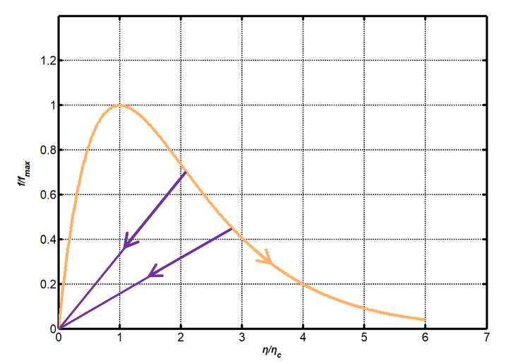
For nonlocal cohesive media under finite deformation, we can also introduce the following Smith-Ferrante type potential function [19] as an alternative mesoscale potential for the nonlocal cohesive continuum, which provides a universal binding potential that can be also written as,

\phi(\boldsymbol{\eta},\boldsymbol{\xi})=\phi_{n}\sigma_{c}e\eta_{c}\left[1-\bigl(1+\frac{\left|\boldsymbol{\eta}\right|}{\eta_{c}}\bigr)\exp\bigl(-\frac{\left|\boldsymbol{\eta}\right|}{\eta_{c}}\bigr)\right]~.

(52)

and its corresponding force equals to

{\bf f}(\boldsymbol{\eta})=\frac{\partial\phi}{\partial{\mbox{\boldmath$\eta$}}}=\phi_{n}\sigma_{c}\exp\Bigl(1-\frac{\left|\boldsymbol{\eta}\right|}{\eta_{c}}\Bigr)\frac{\boldsymbol{\eta}}{\eta_{c}}

(53)

where $\eta_{c}=|{\mbox{\boldmath$\eta$}}_{c}|$ is the critical value, and when ${\mbox{\boldmath$\eta$}}={\mbox{\boldmath$\eta$}}_{c}$ the bond force,

{\bf f}={\partial\phi\over\partial{\mbox{\boldmath$\eta$}}}\Bigm|_{{\mbox{\boldmath$\eta$}}={\mbox{\boldmath$\eta$}}_{c}}~\to~{\bf t}_{max}

reaches its peak value.

In the elastic range, we can also derive the expression of the bond force vector as follows,

{\bf f}(\boldsymbol{\eta})=\frac{\partial\phi}{\partial{\mbox{\boldmath$\eta$}}}=\phi_{n}\sigma_{c}\exp\Bigl(1-\frac{\left|\boldsymbol{\eta}\right|}{\eta_{c}}\Bigr)\frac{\boldsymbol{\eta}}{\eta_{c}}

(54)

The magnitude of the bond force $f=|{\bf f}|$ can be defined as

f=\frac{\partial\phi}{\partial\eta}=\phi_{n}e\sigma_{c}\frac{\eta}{\eta_{c}}\exp\bigl({-\frac{\eta}{\eta_{c}}}\bigr)

(55)

and the normal and tangential components of the bond force can be derived in the following:

f_{n}=\frac{\partial\phi}{\partial\eta_{n}}=\frac{\phi_{n}\eta_{n}\sigma_{c}\exp\bigl(1-\frac{\eta}{\eta_{c}}\bigr)}{\eta_{c}};~{\rm and}~~~f_{t}=\frac{\partial\phi}{\partial\eta_{t}}=\frac{\phi_{n}\eta_{t}\sigma_{c}\exp\bigl(1-\frac{\eta}{\eta_{c}}\bigr)}{\eta_{c}}~.

(56)

It is straightforward to show that:

\boldsymbol{f}=\boldsymbol{f}_{n}+\boldsymbol{f}_{t}

(57)

The derivative of the scalar amplitude bond force relative to $\eta$ is:

\frac{df}{d\eta}=-{\phi_{n}\over\eta_{c}^{2}}\bigl(e\sigma_{c}\exp\bigl({-\frac{\eta}{\eta_{c}}}(\eta-\eta_{c})\bigr)~.

(58)

Equation (58) indicates that the bond force $f$ reaches its maximum when $\eta=\eta_{c}$ . We expediently assume that for the case where $\eta\leq\eta_{c}$ , the material is in elastic phase, and when $\eta\geq\eta_{c}$ the material is in inelastic phase. Also, this conclusion is invariant under coordinate transformation.

Considering the nonlocal strain energy density as follows

W(\boldsymbol{X})=\frac{1}{2V_{\mathcal{H}}}\int_{\mathcal{H}}\int_{\mathcal{H}}\phi(\boldsymbol{\eta},\boldsymbol{\xi})d{\bf X}^{\prime}d{\bf X}^{\prime\prime}

(59)

we can then derive the first Piola-Kirchhoff stress tensor at the location of ${\bf X}$ as

$\displaystyle\boldsymbol{P}(\boldsymbol{X})$	$\displaystyle=$	$\displaystyle\frac{\partial W(\boldsymbol{X})}{\partial\boldsymbol{F}}=\frac{1}{2V_{\mathcal{H}}}\int_{\mathcal{H}}\int_{\mathcal{H}}\frac{\partial\phi(\boldsymbol{\eta},\boldsymbol{\xi})}{\partial\|\boldsymbol{\eta}\|}\frac{\partial\boldsymbol{\|\eta}\|}{\partial\boldsymbol{\eta}}\frac{\partial\boldsymbol{\eta}}{\partial\boldsymbol{F}}d{\bf X}^{\prime}d{\bf X}^{\prime\prime}$	(60)
	$\displaystyle=$	$\displaystyle\frac{1}{2V_{\mathcal{H}}}\int_{\mathcal{H}}\int_{\mathcal{H}}\Bigl[\phi_{n}\sigma_{c}\exp\Bigl(1-\frac{\|\boldsymbol{\eta}\|}{\|\boldsymbol{\eta}\|_{c}}\Bigr){\boldsymbol{\eta}\otimes\boldsymbol{\xi}\over\|\boldsymbol{\eta}\|_{c}}\Bigr]d{\bf X}^{\prime}d{\bf X}^{\prime\prime}$
	$\displaystyle=$	$\displaystyle\frac{1}{2}\int_{\mathcal{H}}\Bigl[\bar{\bf f}\otimes\boldsymbol{\xi}\Bigr]d{\bf X}^{\prime}~$

Accordingly, we can find the elasticity tensor for Smith-Ferrante type cohesive continuum media as

One may find that the initial elastic tensor is given as

\mathbb{C}_{SF}({\bf 0})=\frac{1}{2}\int_{\mathcal{H}}\frac{\phi_{n}\sigma_{c}}{\eta_{c}}\Bigl(\boldsymbol{I}^{(2)}\otimes{\boldsymbol{\xi}}\otimes\boldsymbol{\xi}\Bigr)dV_{\boldsymbol{X}},

(62)

which does not possess the initial shear modulus. This is because the Smith-Ferrante potential is an atomistic pair bond potential that does not have tangential bond displacement initially.

3.4 Determination of characteristic lengths

One of distinguished features of the cohesive continuum is its internal length scale. For the Xu-Needleman potential, $\delta_{n}$ and $\delta_{t}$ are two characteristic length scales that are defined as the maximum elastic bond stretches, i.e.

	$\displaystyle\delta_{n}(\boldsymbol{\xi})$	$\displaystyle=$	$\displaystyle\left\|\boldsymbol{\xi}\right\|c_{n},$		(63)
	$\displaystyle\delta_{t}(\boldsymbol{\xi})$	$\displaystyle=$	$\displaystyle\left\|\boldsymbol{\xi}\right\|c_{t},$		(64)

where $c_{n}$ and $c_{t}$ are the two maximum elastic strains for normal and tangential deformations of a pair bond, respectively. Comparing with the treatment in [1], we can also define two critical bond strains or stretches $s_{n}$ and $s_{t}$ for determining the critical or maximum stretches of the bond: $\delta_{nc}$ and $\delta_{tc}$ :

	$\displaystyle\delta_{nc}(\boldsymbol{\xi})$	$\displaystyle=$	$\displaystyle\left\|\boldsymbol{\xi}\right\|s_{n},$		(65)
	$\displaystyle\delta_{tc}(\boldsymbol{\xi})$	$\displaystyle=$	$\displaystyle\left\|\boldsymbol{\xi}\right\|s_{t},$		(66)

where $s_{n}$ and $s_{t}$ are the critical bond strains or stretches before the bond is broken.

Before, we determine the critical stretches, we first note that the cohesive elastic potential of a Xu-Needleman bond may be interpreted as the elastic bond energy when the bond force reaches to the peak loading forces, which can be obtained as follows,

\displaystyle\phi_{Ie}

\displaystyle=

\displaystyle{\phi_{n}}\left\{1+\displaystyle\exp\bigl(-{1}\bigr)\left\{\bigl[\displaystyle 1-r+{1}\bigr]{\frac{1-q}{r-1}}-\bigl[\displaystyle q+(\frac{r-q}{r-1})\bigr]\right\}\right\}=\frac{e-2}{e}\phi_{n}~

(67)

and

\displaystyle\phi_{IIe}

\displaystyle=

\displaystyle{\phi_{n}}\left\{1+\displaystyle\left\{\bigl[\displaystyle 1-r\bigr]{\frac{1-q}{r-1}}\displaystyle-q\exp\bigl(-1\bigr)\right\}\right\}=\frac{e-1}{e}q\phi_{n}~

(68)

To determine the critical stretches, we adopt the criteria of the critical energy release. It is assumed that the critical energy releases are achieved when all the bonds connecting to the center particle of a given horizon reach their corresponding critical stretches. We assume that the critical stretch of the normal deformation of pairs of bonds is $s_{n}$ , while the corresponding shear critical stretch is $s_{t}$ , therefore the critical values of the cohesive energy for each bond can be found as follows,

$\displaystyle\phi_{Ic}$	$\displaystyle=$	$\displaystyle{\phi_{n}}\left\{1+\displaystyle\exp\bigl(-{\frac{s_{n}}{c_{n}}}\bigr)\left\{(\displaystyle 1-r+{\frac{s_{n}}{c_{n}}}){\frac{1-q}{r-1}}-\bigl[\displaystyle q+(\frac{r-q}{r-1}){\frac{s_{n}}{c_{n}}}\bigr]\right\}\right\}~$	(69)
	$\displaystyle=$	$\displaystyle\frac{1}{2}\phi_{n}\left[1-\Bigl(1+{\lambda_{n}^{-1}}\Bigr)\exp{(-\lambda_{n})}\right]$	(69)
$\displaystyle\phi_{IIc}$	$\displaystyle=$	$\displaystyle{\phi_{n}}\left\{1+\displaystyle\left\{(\displaystyle 1-r){\frac{1-q}{r-1}}-\displaystyle q\exp\bigl(-{s_{t}^{2}\over c_{t}^{2}}\bigr)\right\}\right\}$	(70)
	$\displaystyle=$	$\displaystyle\frac{1}{2}q\phi_{n}\left[1-\exp{(-\lambda_{t}^{2})}\right]$	(70)

where we define

s_{n}:=\lambda_{n}c_{m}~~~{\rm and}~~~~s_{t}:=\lambda_{t}c_{t}

(71)

which are amplitude factors for critical stretches.

Following [20, 21], the corresponding energy releases can be related to the critical cohesive energy under both tensile and shear deformation mode as follows,

	$\displaystyle G_{I0}(\lambda_{n})$	$\displaystyle=$	$\displaystyle\int_{0}^{H}\int_{0}^{2\pi}\int_{z}^{H}\int_{0}^{\cos^{-1}(z/\xi)}\phi_{Ic}(\lambda_{n})\xi^{2}\sin\psi d\psi d\xi d\theta dz~$		(72)
	$\displaystyle G_{II0}(\lambda_{t})$	$\displaystyle=$	$\displaystyle\int_{0}^{H}\int_{0}^{2\pi}\int_{z}^{H}\int_{0}^{\cos^{-1}(z/\xi)}\phi_{IIc}(\lambda_{t})\xi^{2}\sin\psi d\psi d\xi d\theta dz$		(73)

The above integrations are performed in an integration domain shown in Fig. 5. Based on the above equations, we can find critical stretches $s_{n}$ and $s_{t}$ by implicitly solving two nonlinear algebraic equations:

G_{Ic}-G_{I0}(\lambda_{n})=0,~~{\rm and}~~G_{IIc}-G_{II0}(\lambda_{t})=0~.

(74)

Remark 3.3

In the proposed cohesive peridynamics modeling (CPDM), the critical stretch is not necessary concept. This is because that the functional form of the mesoscale cohesive potential implicitly determines the critical stretch — that is the critical stretch is a part of the cohesive potential, and one does not need extra effort to break a bond. All the material bond can be broken naturally without user interference. However, the determination of $\lambda_{s}$ and $\lambda_{t}$ can help to set up the cutoff distance. In this sense, the cutoff distance of the material bond should be chosen as

\ell_{c}=s_{c}\ell_{\xi},~~{\rm where}~~s_{c}=min(\lambda_{n}c_{n},\lambda_{t}c_{t}).

4 Cohesive stress and peridynamic stress

A main task of cohesive nonlocal continuum mechanics is to find the underline cohesive continuum stress measures based on the bond deformation and its corresponding bond force. This is the step of micro to macro transition, which bridges the mesoscale description and the macroscale description. This will help us to understand a host of physical phenomena from different perspectives, such as the crack growth criterion [21].

To proceed, we first recall Eq. (31),

\displaystyle\boldsymbol{P}(\boldsymbol{X})

\displaystyle=

\displaystyle\frac{\partial W(\boldsymbol{X})}{\partial\boldsymbol{F}}=\frac{1}{2}\int_{\mathcal{H}}\Bigl[\bar{\bf f}\otimes\boldsymbol{\xi}\Bigr]dV_{\boldsymbol{\xi}}~

(75)

Consider the following peridynamic force sampling formula,

\bar{\bf f}({\bf X}^{\prime},{\bf X})=\sum_{I=1}^{N}\sum_{J=1,J\not=I}^{N}{\bf t}_{IJ}w({\bf X}_{I}-{\bf X})\delta(({\bf X}_{J}-{\bf X}_{I})-({\bf X}^{\prime}-{\bf X}))~.

(76)

where ${\bf X},{\bf X}^{\prime},{\bf X}_{I}$ and ${\bf X}_{J}$ are material particles in the referential configuration, ${\bf t}_{IJ}$ is the bond force (not the force state) acting on the particle ${\bf X}_{I}$ from the particle ${\bf X}_{J}$ .

By substituting the force sampling expression in Eq. (76) into Eq. (75), we have

	$\displaystyle{\bf P}({\bf X})$	$\displaystyle=$	$\displaystyle\frac{1}{2}\int_{\mathcal{H}}\Bigl[\bar{\bf f}\otimes\boldsymbol{\xi}\Bigr]dV_{{\xi}}$		(77)
		$\displaystyle=$	$\displaystyle\frac{1}{2}\int_{\mathcal{H}}\sum_{I=1}^{N}\sum_{J=1,J\not=I}^{N}w({\bf X}_{I}-{\bf X}){\bf t}_{IJ}\otimes{\mbox{\boldmath$\xi$}}\delta(({\bf X}_{J}-{\bf X}_{I})-({\bf X}^{\prime}-{\bf X}))dV_{{\xi}}~.$		(77)

For simplicity, we may choose the radial step function as the sampling function, i.e.

w(r)=\left\{\begin{array}[]{lcl}\displaystyle{1\over\Omega_{X}},&&r<\delta\\ \\ 0,&&{\rm otherwise}\end{array}\right.

(78)

where $\Omega_{X}=\mathcal{H}_{X}$ and $vol(\mathcal{H}_{X})=(4/3)\pi H^{3}$ , and $H$ is the radius of the horizon.

Since ${\bf X},{\bf X}_{I}\in\mathcal{H}_{X}$ , $w({\bf X}_{I}-{\bf X})=1$ . We then have the mathematical expression of the cohesive first Piola-Kirchhoff stress,

In 2008, based on Noll’s lemma [22], Lehoucq and Silling [10] proposed a peridynamic stress [10],

{\bf P}_{LS}({\bf X}):={1\over 2}\int_{\mathcal{S}^{2}}\int_{0}^{\infty}\int_{0}^{\infty}(y+z)^{2}{\bf f}({\bf X}+y{\bf M},{\bf X}-z{\bf M})\otimes{\bf M}dzdyd\Omega_{M}~,

(80)

where $\mathcal{S}^{2}$ is the unit sphere.

Now, we show that the cohesive stress derived in Eq. (79) is exactly the same as the peridynamic stress defined by Lehoucq and Silling [10], i.e.

{\bf P}_{coh}={\bf P}_{LS}~.

Theorem 4.1 (Peridynamic Stress)

Assume that the average Peridynamic force density in a horizon that can be expressed as the following discrete sampling expression of the Irving-Kirkwood-Hardy formulation [4, 23, 24],

\bar{\bf f}({\bf X},{\bf X}^{\prime})=\sum_{I=1}^{N_{X}}\sum_{J=1,J\not=I}^{N_{X}}{\bf t}_{IJ}w({\bf X}_{I}-{\bf X})\delta(({\bf X}_{J}-{\bf X}_{I})-({\bf X}^{\prime}-{\bf X})),

(81)

where ${\bf X},{\bf X}^{\prime},{\bf X}_{I}$ and ${\bf X}_{J}$ are material particles in the referential configuration, ${\bf t}_{IJ}$ is the force (not the force state) acting on the particle ${\bf X}_{I}$ from the particle ${\bf X}_{J}$ (see Fig. 6), $N_{X}$ is the total number of particles inside the horizon $\mathcal{H}_{X}$ , $\delta({\bf X})$ is the Dirac delta function, and $w({\bf X}_{I}-{\bf X})$ is a window function or kernel function.

The nonlocal peridynamic stress defined by Lehoucq and Silling [10]

{\bf P}_{LS}:={1\over 2}\int_{\mathcal{S}^{2}}\int_{0}^{\infty}\int_{0}^{\infty}(y+z)^{2}{\bf f}({\bf X}+y{\bf M},{\bf X}-z{\bf M})\otimes{\bf M}dzdyd\Omega_{M}~,

(82)

can be expressed the following discrete summation form,

{\bf P}_{LS}({\bf X}):={1\over 2}\sum_{I=1}^{N_{X}}\sum_{J=1,J\not=I}^{N_{X}}{\bf t}_{IJ}\otimes({\bf X}_{J}-{\bf X}_{I})B_{IJ}({\bf X}),~~{\bf X}_{I},{\bf X}_{J}\in\mathcal{H}_{X},~~

(83)

where ${\bf X}$ is the center point of the horizon $\mathcal{H}_{X}$ and ${\bf X}\in\mathcal{B}$ , ${\bf t}_{IJ}={\bf f}({\bf X}_{J},{\bf X}_{I})V_{I}V_{J}$ is the force acting on the particle ${\bf X}_{I}$ by the particle ${\bf X}_{J}$ , where ${\bf X}_{I},{\bf X}_{J}\in\mathcal{H}_{X}$ , $V_{I}$ and $V_{J}$ represents the volume of material particle ${\bf X}_{I}$ and ${\bf X}_{J}$ , respectively, as shown in Fig. 6, and

B_{IJ}({\bf X})=\int_{0}^{1}w(\alpha({\bf X}_{J}-{\bf X}_{I})+{\bf X}_{I}-{\bf X})d\alpha

(84)

is the bond function.

Based on Noll’s lemma [22], we can write the first peridynamics Piola-Kirchhoff stress as

	$\displaystyle{\bf P}_{LS}({\bf X})$	$\displaystyle=$	$\displaystyle{1\over 2}\int_{\mathcal{S}^{2}}d\Omega_{m}\int_{0}^{\infty}R^{2}dR\int_{0}^{1}{\bf f}({\bf X}+\alpha R{\bf M},{\bf X}-(1-\alpha)R{\bf M})\otimes{\bf M}d\alpha$		(85)
		$\displaystyle=$	$\displaystyle-{1\over 2}\int_{3}dV_{R}\int_{0}^{1}{\bf f}({\bf X}+\alpha{\bf R},{\bf X}-(1-\alpha){\bf R})\otimes{\bf R}d\alpha~,~\forall{\bf X}\in\mathcal{B}$		(85)

Considering the Hardy-Murdoch procedure [24, 25, 26], we have the following peridynamics sampling formulation (see Fig. 1)

{\bf f}({\bf X}^{\prime},{\bf X})=\sum_{I=1}^{N_{X}}\sum_{J=1,J\not=I}^{N_{X}}{\bf t}_{IJ}w({\bf X}_{I}-{\bf X})\delta(({\bf X}_{J}-{\bf X}_{I})-({\bf X}^{\prime}-{\bf X})),~~

(86)

where the window function, or sampling function, must satisfy the following conditions,

\int_{\mathcal{H}_{X}}w({\bf y}-{\bf x})dV_{y}=1~,

(87)

and

\lim_{r\to 0}w(r)~\to~\delta(r)~.

(88)

Condition (87) is the averaging requirement, and Condition (88) ensures that the Dirac comb sampling can converge to a correct continuum form of integrand in Eq. (3), i.e.

\sum_{I=1}^{N_{X}}\sum_{J=1,J\not=I}^{N_{X}}{\bf t}_{IJ}w({\bf X}_{I}-{\bf X})\delta(({\bf X}_{J}-{\bf X}_{I})-({\bf X}^{\prime}-{\bf X}))~\to~{\bf f}({\bf X},{\bf X}^{\prime}-{\bf X})~.

Letting

{\bf X}={\bf X}+\alpha{\bf R},~{\rm and}~~{\bf X}^{\prime}={\bf X}-(1-\alpha){\bf R}

and substituting them into Eq. (86), we then have

			$\displaystyle{\bf f}({\bf X}+\alpha{\bf R},{\bf X}-(1-\alpha){\bf R})$		(89)
		$\displaystyle=$	$\displaystyle\sum_{I=1}^{N_{X}}\sum_{J=1,J\not=I}^{N_{X}}{\bf t}_{IJ}w(({\bf X}_{I}-{\bf X})-\alpha{\bf R})\delta({\bf R}-({\bf X}_{I}-{\bf X}_{J})),$		(89)

where ${\bf X}_{I},{\bf X}_{J}\in\mathcal{H}_{X_{C}},~~{\bf X}_{I}\not={\bf X}_{J}$ .

Considering the following integration identities

\displaystyle\int_{-\infty}^{\infty}\delta(\xi-x)w(x-\eta)dx=w(\xi-\eta),

(90)

we first integrate

	$\displaystyle\int^{3}\delta({\bf R}-({\bf X}_{I}-{\bf X}_{J}))w(({\bf X}_{I}-{\bf X}))-\alpha{\bf R}){\bf R}dV_{R}$
	$\displaystyle=({\bf X}_{I}-{\bf X}_{J})w\bigl(({\bf X}_{I}-{\bf X})-\alpha({\bf X}_{I}-{\bf X}_{J})\bigr)~.$		(91)

Following [24], we may define the second integral as the so-called bond function, i.e.

B_{IJ}({\bf X})=\int_{0}^{1}w(\alpha({\bf X}_{J}-{\bf X}_{I})+{\bf X}_{I}-{\bf X})d\alpha

(92)

Thus, we have

\displaystyle{\bf P}_{LS}({\bf X})

\displaystyle=

\displaystyle{1\over 2}\bigl(\sum_{I=1}^{N_{X}}\sum_{J=1,J\not=I}^{N_{X}}{\bf t}_{IJ}\otimes({\bf X}_{J}-{\bf X}_{I})\bigr)B_{IJ}({\bf X})~,

(93)

which is called the Hardy stress (see [24, 27].

If we choose $w({\bf x})$ as the spherical radial step function (see Eq. (78)), one can see that

w(\alpha({\bf X}_{J}-{\bf X}_{I})+{\bf X}_{I}-{\bf X})=w(\alpha({\bf X}_{J}-{\bf X})+(1-\alpha)({\bf X}_{I}-{\bf X}))~.

If ${\bf X}_{I},{\bf X}_{J}\in\mathcal{H}_{X}$ , we can see that

{\bf X}_{x\alpha}:=\alpha({\bf X}_{J}-{\bf X})+(1-\alpha)({\bf X}_{I}-{\bf X})\in\mathcal{H}_{X}

This is because that

|\alpha({\bf X}_{J}-{\bf X})+(1-\alpha)({\bf X}_{I}-{\bf X})|\leq|\alpha({\bf X}_{J}-{\bf X})+(1-\alpha)({\bf X}_{J}-{\bf X})|=|{\bf X}_{J}-{\bf X}|\leq\delta

if $|{\bf X}_{J}-{\bf X}|\geq|{\bf X}_{I}-{\bf X}|$ , and vice vera

|\alpha({\bf X}_{J}-{\bf X})+(1-\alpha)({\bf X}_{I}-{\bf X})|\leq|\alpha({\bf X}_{I}-{\bf X})+(1-\alpha)({\bf X}_{I}-{\bf X})|=|{\bf X}_{I}-{\bf X}|\leq\delta

if $|{\bf X}_{J}-{\bf X}|\leq|{\bf X}_{I}-{\bf X}|$ as shown in Fig. 7.

Thus, it is readily to show that

B_{IJ}({\bf X})={1\over\Omega_{X}},~~~~{\rm if}~{\bf X}_{I},{\bf X}_{J}\in\mathcal{H}_{X}

For this special case, the peridynamic stress has the expression,

Equation (94) confirms that the peridynamic stress is the first Piola-Kirchhoff virial stress, or it is equal to the cohesive first Piola-Kirchhoff stress.

5 Numerical examples

In this section, we present several numerical examples to validate the proposed CPDM method. All the 2D models or examples are computed under 2D plane stress conditions using uniform particles. For the 3D example, we conducted a three-point bending beam test, which is widely used to investigate mix-mode fracture behavior. Force-displacement curves for all cases are compared with experimental results.

5.1 Two-dimensional crack growth

In this example, we used CPDM to simulate a 2D crack growth problem to validate the proposed CPDM method. The specimen size and boundary condition setting are shown in Fig.8. The morphology of the specimen after complete fracture is shown as the result diagram in Fig. 9, and the color contour represents $S_{22}$ distribution (PK-II stress component in y-direction).

An advantage of using cohesive mesoscale potential is that by adjusting the numerical values of the parameters we can observe both brittle and ductile fracture as well as their transition . For example, by adjusting the ratio of the parameter $\delta_{n}$ to $\delta_{t}$ , the simulated crack shape changes from ductile fracture to brittle fracture as shown in Fig. 9.

It can be seen from Fig.9 that from $(a)$ to $(e)$ with the increase of the ratio of $\delta_{n}/\delta_{t}$ , the feature of the brittle fracture gradually becomes obvious. We also compared the calculation results of CPDM with those of FEM-CZM, which are shown in Fig. 10. The ratio of $\delta_{n}/\delta_{t}$ in the comparison example is chosen as 0.2. From 10, one may find that that the two results are in a good agreement.

In addition, we also simulated the transit effect of the stress evolution at the crack tip during the crack propagation by using the notched specimen. Figure 11 shows the stress distribution of $S_{22}$ at the crack tip from the moment of crack initiation to the stage that crack propagated well into the middle . In this case, the ratio of $\delta_{n}/\delta_{n}$ is chosen as 1.

5.2 Trunk’s test: Wedge splitting fracture

In 1999, Trunk [28] conducted an experimental investigation into the size dependence of non-linear fracture mechanics parameters for cementitious materials. The wedge splitting test is adopted in his research, which was later widely replicated for the purpose of verifying and validating various fracture simulations. In this work, we also conducted a numerical experiment of Trunk’s test by using the proposed CPDM method to simulate wedge splitting fracture test.

The geometry and boundary conditions are depicted in Fig. 12, and the dimensions of the square-shaped specimen is chosen as 400mm $\times$ 400mm $\times$ 400mm, while the width of the prefabricated crack is $10mm$ . Other geometric parameters are shown in Fig.12. The material properties of the specimen adopted in the simulation are given as follows: Young’ modules $E=28.3Gpa$ , Poisson’s ratio $\nu=0.2$ , and the fracture energy release $G_{f}=0.017n/mm$ . The specimen is subjected to a prescribed force at left and right side, while the bottom of the specimen is fixed. The particle spacing is $\Delta=5mm$ , and the horizon radius $\delta$ is equal to 3 $\Delta$ .

The simulated wedge crack splitting process is shown in Fig. 13 with damage color contour and in Fig. 14 with the stress color contour. The sequences reflect the damage of the specimen and stress variables at different time instances in the simulation.

Figure 13 shows the change of damage contour with respect to time. Material damage is calculated for each material point. In traditional PD method, for each material point, when the elongation of the bond between the two material points exceeds the critical stretch $s_{0}$ , the irreversible fracture or bond breaking will occur. We call the ratio of the number of broken bonds to the total number of bonds of a material point its damage [29], i.e.

d({\bf X})=1-{\int_{\mathcal{H}_{X}}\mu({\bf X},{\bf X}^{\prime})dV_{{\bf X}^{\prime}}\over\int_{\mathcal{H}_{X}}dV_{{\bf X}^{\prime}}}

where

\mu({\bf X},{\bf X}^{\prime})=\left\{\begin{array}[]{ll}1&~{\rm if}~\overline{{\bf X}{\bf X}^{\prime}}~{\rm bond~is~broken}\\ \\ 0&~{\rm if}~\overline{{\bf X}{\bf X}^{\prime}}~{\rm bond~is~not~broken}\end{array}\right.

is the characteristic function of the material bond.

When the damage factor of a material point is 1, it means that all bonds are not damaged. When the damage factor is equal to 0, it means that the material point has been completely damaged. As shown in Fig. 13, the wedge specimen began suffering damages in about 1ms, and it was tore obviously at the middle prefabricated crack in about 1.5ms, and the specimen was completely torn apart after 1.75ms. The stress evolution process is shown in Fig.14, and the stress evolution process is basically consistent with that of the damage evolution.

5.3 Fracture of L-shape plate

In this example, to validate the proposed CPDM, we apply it simulating the fracture of a L-shape concrete plate, which was studied in [30] by using a finite element analysis of elasto-plastic damage constitutive modeling.

The geometry and boundary conditions of the L shape plate are depicted in Fig. 15. As shown in the figure, L shape plate side length is 500mm, the bottom end is a fixed boundary, and there is an upward force on the right bottom edge. The material properties of the plate are chosen as follows: $E=25.85Gpa$ , $\mu$ = $0.2$ and $G_{f}=0.015N/mm$ . In the numerical simulations, the spacing between particles is $5mm$ .

To validate the proposed CPDM formulation, the L-shape plate has the same dimension and material constants used in 16, except that we adopt the Xu-Needleman cohesive potential rather an elasto-plastic damage model, while using nonlocal cohesive peridyanmics rather than finite element crack smearing techniques. Fig.17 show the damage and stress distribution of the L-shape plate. It can be clearly seen from the resulting figure that at $5.22ms$ , the crack originated at the right angle and gradually extended to the left side,the L shape plate began to suffer damage at the bend corner, and stress concentration also appeared at the bend corner in Fig. 17. The stress at the right margin in Fig. 17 is obviously greater than the rest of the plate because this is where the external force is applied, this is why this area also appear some damage.

5.4 Plate with the hole

In this example, we employed CPDM carrying out numerical simulation of a thin plate with hole under uniaxial tension, which is under plane stress condition. For infinitesimal deformation, this problem has a close-form solution, i.e. the well-known Kirsch solution [31].

The geometry and boundary setting are shown in Fig. 18. The side length of the square plate is 100 mm, and a circular hole with a radius of 5 mm is opened in the center of the square plate. In the numerical simulations,the spacing between particles is $5mm$ . In addition, in order to verify the convergence of CPDM, we also use this example to compare CPDM results with analysis values. The analytical Kirsch’s solution of stress components around a circular hole in an elastic infinite plate under tension are give as follows,

$\displaystyle\sigma_{rr}$	$\displaystyle=$	$\displaystyle\frac{\sigma_{0}}{2}(1-\frac{a^{2}}{r^{2}})+\frac{\sigma_{0}}{2}(1-\frac{a^{2}}{r^{2}})(1-3\frac{a^{2}}{r^{2}})\cos 2\theta$	(95)
$\displaystyle\sigma_{\theta\theta}$	$\displaystyle=$	$\displaystyle\frac{\sigma_{0}}{2}(1+\frac{a^{2}}{r^{2}})-\frac{\sigma_{0}}{2}(1+3\frac{a^{4}}{r^{4}})\cos 2\theta$	(96)
$\displaystyle\sigma_{r\theta}$	$\displaystyle=$	$\displaystyle\sigma_{\theta r}=-\frac{\sigma_{0}}{2}(1-\frac{a^{2}}{r^{2}})(1+3\frac{a^{2}}{r^{2}})sin2\theta$	(97)

where $\theta$ and $r$ are the polar coordinates measured form the center of the circular hole. $r$ is the radial distance of the point of interests to the center of the hole, and $\theta$ is the angle between the x-axis and the radial vector ${\bf r}$ as shown in Fig. 17. The comparison between the CPDM solution and the analytical Kirsch’s solution given shown in Fig.19.

This example not only validate CPDM method, but also validate and verify the cohesive stress formulation derived in this paper. The variation of stress distribution is shown in Fig. 20.

5.5 Double-edge notched specimen test

In this example, we conducted a numerical simulation of a double-edge notched specimen under tensile loading, which was based on the experiment reported in [32]. In the original experiment, the notch was set to be asymmetric, and hence it is a mixed-mode fracture. This example provides us an opportunity to test how CPDM to handle mixed mode fracture.

The problem setting is displayed in the Fig. 21. The numerical specimen is $120mm$ long and $60mm$ wide. Two notches are set respectively at two lateral sides with $5mm$ from the middle line from above and below. Each notch is $10mm$ long and $2mm$ wide. The material parameters of the specimen are: $E=40GP_{a}$ , $\mu=0.2$ , and $G_{f}=0.025N/mm$ . The particle spacing in the numerical simulation is chosen as $5mm$ , and the horizon size is taken as $3.015$ times the particle spacing.

Figure 22 shows the sequence of crack growth with the damage contour at different time instances, while Fig. 23 displays the sequence of crack growth with the stress $S_{22}$ contour.

5.6 Three point bending test

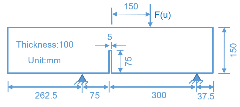
The third example is a three-dimensional (3D) simulation of cohesive peridynamics, in which we conducted a numerical test of the three-point bending of a beam [33]. This example is widely used as a benchmark problem of 3D mixed mode fracture. The simulation domain and boundary condition are shown in Fig.24. The material properties are set as follows: the Young’ modules $E=20GP_{a}$ ; Poisson’s ratio $\nu$ = $0.2$ ; and the fracture energy $G_{f}=0.015N/mm$ . A concentrated downward load is acted at the upper midpoint of the beam, and the left and right ends of the lower part are fixed by the fixative structure. In the numerical simulations, the spacing between particles is chosen $5mm$ . The 3D numerical specimen is shown in Fig.25.

We plot the fracture process of the simply supported beam in Fig.26. Figure 26 (a), (b), and (c) show the stress distribution of the beam at different time instances during the loading, and Fig.27 (a), (b), and (c) shows the damage evolution with respect to the time.

Fig.28 shows the change of force with respect to crack mouth opening displacement (CMOD). In Fig.28, the dotted line represents the numerical calculation result obtained by using the cohesive peridynamics and the gray area shows the experiment data, the other lines present the results obtained by using the extended finite element (eXFEM) and the state-based peridynamics that is mislabeled as the cohesive zone peridynamics method.

6 Discussions and conclusions

It has been almost four decades since Xu and Needleman’s pioneer work on cohesive zone model (CZM) [11], and finite element CZM method established itself as a primary numerical method to model inelastic fracture at small scale yielding.

However, CZM has some technical issues such as mesh dependence, adaptive mesh refinement, and modeling on mixed mode fracture, among others. Among these shortcomings, one of the major criticisms on CZM is its replacement of a homogeneous material by a cohesive interface “composite” in its core mechanics model. On the other hand, the cohesive peridynamics model (CPDM) proposed in this work is a nonlocal cohesive continuum mechanics, and it has demonstrated its potential to address all the issues mentioned above, which exist in finite element cohesive zone model. Moreover, unlike the prototype micro-brittle (PMB) model in the bond-based peridynamics, the bond-based cohesive peridynamics model (CPDM) has variable Poisson’s ratio, does not need the critical stretch parameter $s_{0}$ , and provides intrinsic stress measure that is consistent with strain measure in the bulk homogeneous continua. Thus, CPDM is a bona fide nonlocal cohesive continuum mechanics modeling.

Furthermore, in this work, we have shown in the first time that the elastic tensor derived from the mesoscale pairwise Xu-Needleman potential is not limited by the Cauchy relation. This stunning discovery will greatly broaden applications of the bond-based peridynamics.

It should be mentioned that in the literature some authors labeled their state-based peridynamics or coupling method between finite element method and the state-based peridynamics as the cohesive peridynamics, e.g. [37, 36, 13]. Even though there are some cohesive zone features in these state-based peridynamics, they are not really cohesive peridynamics model, because in those work the micrscale cohesive bond force models do not govern the macroscale constitutive relations. Whereas, in the proposed CPDM model the mesoscale or microscale cohesive bond potential determines the material constitutive relations at macroscale. Therefore, CPDM is a consistent cohesive zone model.

Acknowledgments

The authors would like to thank Dr.Xuan Hu of the University of California, Berkeley for some helpful discussions. J.H and A.Z are supported by the National Natural Science Foundation of China (Grant number 52088102 and 51925904), which are gratefully acknowledged.

References

[1] X. P. Xu and A. Needleman. Void nucleation by inclusion debonding in a crystal matrix. Modelling and Simulation in Materials Science and engineering, 1(2):111–132, 1993.
[2] S.A. Silling. Reformulation of elasticity theory for discontinuities and long-range forces. Journal of the Mechanics and Physics of Solids, 48:175–209, 2000.
[3] S.A. Silling, M. Epton, O. Weckner, J. Xu, and E. Askari. Peridynamic states and constitutive modeling. Journal of Elasticity, 88:151–184, 2007.
[4] S.A. Silling and R.B. Lehoucq. Peridynamic theory of solid mechanics. Advances in Applied Mechanics, 44:73–168, 2010.
[5] S. A. Silling. Linearized theory of peridynamic states. Journal of Elasticity, 99:85–111, 2010.
[6] E. Madenci and E. Oterkus. Peridynamic theory and its applications. Springer, New York, 2014.
[7] T.L. Warren, S.A. Silling, A. Askari, O. Weckner, M.A. Epton, and J. Xu. A non-ordinary state-based peridynamic method to model solid material deformation and fracture. International Journal of Solids and Structures, 46(5):1186–1195, 2009.
[8] M. S. Breitenfeld, P.H. Geubelle, O. Weckner, and S.A. Silling. Non-ordinary state-based peridynamic analysis of stationary crack problems. Computer Methods in Applied Mechanics and Engineering, 272(apr.15):233–250, 2014.
[9] J. Trageser and P. Seleson. Bond-based peridynamics: a tale of two poisson’s ratios. Journal of Peridynamics and Nonlocal Modeling, 2(4), 2020.
[10] R.B. Lehoucq and S.A. Silling. Force flux and the peridynamic stress tensor. Journal of the Mechanics and Physics of Solids, 56(4):1566–1577, 2008.
[11] X.P. Xu and A. Needleman. Numerical simulations of fast crack growth in brittle solids. Journal of the Mechanics and Physics of Solids, 42(9):1397–1434, 1994.
[12] M.S. Breitenfeld. Quasi-static non-ordinary state-based peridynamics for the modeling of 3D fracture. PhD thesis, University of Illinois at Urbana-Champaign, 2014.
[13] D. Yang, X. He, X. Liu, Y. Deng, and X. Huang. A peridynamics-based cohesive zone model (pd-czm) for predicting cohesive crack propagation. International Journal of Mechanical Sciences, 184:105830, 2020.
[14] D. Yang, X. He, J. Zhu, and Z. Bie. A novel damage model in the peridynamics-based cohesive zone method (pd-czm) for mixed mode fracture with its implicit implementation. Computer Methods in Applied Mechanics and Engineering, 377:113721, 2021.
[15] G.L. Bergel and S. Li. The total and updated lagrangian formulation of state-based peridynamics. Computational Mechanics, 58:351–370, 2016.
[16] X. Kan, J. Yan, S. Li, and A-M. Zhang. On differences and comparisons of peridynamic differential operators and nonlocal differential operators. Computational Mechanics, 68:1349–1367, 2021.
[17] J. Yan, S. Li, X. Kan, A. Zhang, and X. Lai. Higher-order nonlocal theory of updated lagrangian particle hydrodynamics (ulph) and simulations of multiphase flows. Computer Methods in Applied Mechanics and Engineering, 368:113176, 2020.
[18] H. Yu and S. Li. On approximation theory of nonlocal differential operators. International Journal for Numerical Methods in Engineering, 122:6984–7012, 2021.
[19] M. Ortiz and A. Pandolfi. Finite-deformation irreversible cohesive elements for three-dimensional crack propagation analysis. International Journal for Numerical Methods in Engineering, 44(9):1267–1282, 1999.
[20] S.A. Silling and E. Askari. A meshfree method based on the peridynamic model of solid mechanics. Computers & structures, 83(17-18):1526–1535, 2005.
[21] H. Yu and S. Li. On energy release rates in peridynamics. Journal of the Mechanics and Physics of Solids, 142:104024, 2020.
[22] W. Noll. Die herleitung der grundgleichungen der thermomechanik der kontinua aus der statistischen mechanik. Journal of Rational Mechanics and Analysis, 4:627–646, 1955.
[23] J.H. Irving and J.G. Kirkwood. The statistical mechanical theory of transport processes. iv. the equations of hydrodynamics. The Journal of Chemical Physics, 18(6):817–829, 1950.
[24] R.J. Hardy. Formulas for determining local properties in molecular-dynamics simulations: Shock waves. The Journal of Chemical Physics, 76(1):622–628, 1982.
[25] A.I. Murdoch. The motivation of continuum concepts and relations from discrete considerations. The Quarterly Journal of Mechanics and Applied Mathematics, 36(2):163–187, 1983.
[26] A.I. Murdoch. A critique of atomistic definitions of the stress tensor. Journal of Elasticity, 88(2):113–140, 2007.
[27] J.A. Zimmerman, E.B. WebbIII, J.J. Hoyt, R.E. Jones, P.A. Klein, and D.J. Bammann. Calculation of stress in atomistic simulation. Modelling and Simulation in Materials Science and Engineering, 12(4):S319, 2004.
[28] B.G. Trunk. Einfluss der Bauteilgrsse auf die Bruchenergie von Beton. PhD thesis, ETH Zurich, 1999.
[29] S. Jafarzadeh, Z. Chen, S. Li, and F. Bobaru. A peridynamic mechano-chemical damage model for stress-assisted corrosion. Electrochimica Acta, 323:134795, 2019.
[30] B Winkler, G Hofstetter, and H Lehar. Application of a constitutive model for concrete to the analysis of a precast segmental tunnel lining. International Journal for Numerical & Analytical Methods in Geomechanics, 28(7-8):797–819, 2010.
[31] E. G. Kirsch. Die theorie der elastizitat und die bedurfnisse der festigkeitslehre. Zeitschrift des Vereines Deutscher Ingenieure, 42, 1898.
[32] C. Shi, A. G. van Dam, J. G. van Mier, and L.J. Sluys. Crack interaction in concrete. In Materials for Buildings and Structures, volume 6, pages 125–131.
[33] JC Gálvez, M. Elices, G. V. Guinea, and J. Planas. Mixed mode fracture of concrete under proportional and nonproportional loading. International Journal of Fracture, 94(3):267–284, 1998.
[34] B. Winkler, G. Hofstetter, and H. Lehar. Application of a constitutive model for concrete to the analysis of a precast segmental tunnel lining. International Journal for Numerical and Analytical Methods in Geomechanics, 28(7-8):797–819, 2010.
[35] J. F. Unger, S. Eckardt, and C. Konke. Modelling of cohesive crack growth in concrete structures with the extended finite element method. Computer Methods in Applied Mechanics and Engineering, 196(41-44):4087–4100, 2007.
[36] D. Yang, X. He, S. Yi, and X. Liu. An improved ordinary state-based peridynamic model for cohesive crack growth in quasi-brittle materials. International Journal of Mechanical Sciences, 153:402–415, 2019.
[37] Y. Tong, W.Q. Shen, and J.F. Shao. An adaptive coupling method of state-based peridynamics theory and finite element method for modeling progressive failure process in cohesive materials. Computer Methods in Applied Mechanics and Engineering, 370:113248, 2020.