A topology optimization of open acoustic waveguides based on a scattering matrix methodJournal: Wave Motion
Abstract
This study presents a topology optimization scheme for realizing a bound state in the continuum along an open acoustic waveguide comprising a periodic array of elastic materials. First, we formulate the periodic problem as a system of linear algebraic equations using a scattering matrix associated with a single unit structure of the waveguide. The scattering matrix is numerically constructed using the boundary element method. Subsequently, we employ the Sakurai–Sugiura method to determine resonant frequencies and the Floquet wavenumbers by solving a nonlinear eigenvalue problem for the linear system. We design the shape and topology of the unit elastic material such that the periodic structure has a real resonant wavenumber at a given frequency by minimizing the imaginary part of the resonant wavenumber. The proposed topology optimization scheme is based on a level-set method with a novel topological derivative. We demonstrate a numerical example of the proposed topology optimization and show that it realizes a bound state in the continuum through some numerical experiments.
Keywords:
Bound state in the continuum , Topology optimization , Acoustic waveguide , Scattering matrix , Boundary element method2010 MSC
00-01, 99-001 Introduction
Recently, bound states in the continuum (BICs) have been enthusiastically investigated in the fields of quantum mechanics, photonics, acoustics, and water waves hsu2016bound. BICs were originally proposed by von Neumann and Wigner vonneumann1929uber in a quantum system and then experimentally found in some classical systems plotnik2011experimental, lee2012observation, hsu2013observation. Historically, it has been said that bound states can exist only outside the radiation continuum, where a near-field state cannot be coupled to any radiation (scattering) channel, resulting in a perfectly confined state in the vicinity of a structure. Challenging this conventional wisdom, BICs may exist within the continuum in some geometrical systems, e.g., waveguides linton2007embedded, dreisow2009adiabatic and photonic/phononic crystal slabs (diffraction gratings) lee2012observation, hsu2013observation, yang2014analytical, bulgakov2014bloch. BICs are of theoretical interest and practical importance due to their potential to realize high-Q resonance, which is an essential property of lasers kodigala2017lasing, filters foley2014symmetryprotected, and sensors yanik2011seeing for next generations.
Because resonance properties are sensitive to the material and geometrical configurations of a structure, some inverse-design approaches, such as parameter tuning and shape/topology optimization sokolowski1992introduction, bendsoe2013topology, may be necessary to realize high-Q resonance originating from BICs in practical applications hsu2016bound. Such optimization techniques have been recently used to design some photonic and phononic structures with maximized bandgaps dobson1999maximizing. Though BICs are formulated similar to photonic/phononic bandgaps, we encounter some numerical difficulties when applying optimization-based design methods to manipulate BICs because they often rely on finite element methods.
BICs are formulated as resonant states satisfying Maxwell’s or Helmholtz’ equations in open systems and characterized as an eigenmode of a nonlinear eigenvalue problem to find a frequency and wavenumber that allow a nonzero state without any incident field. For some simple geometries, we can employ a semianalytical technique, such as cylindrical or spherical wave expansions bulgakov2014bloch, to effectively compute resonant states. For example, Evans and Porter showed numerical evidence that a circular inclusion in a planar waveguide supports BICs evans1998trapped. Later, rectangular scatterers are considered by Porter and Evans porter2005embedded. The recent work by Bennetts and Peter investigated arrays of circular scatterers in water based on a transfer operator with cylindrical functions bennetts2022rayleigh. See the review by Linton and McIver for more details linton2007embedded. However, more general configurations require a discretization-based method, such as the finite element method and boundary element method (BEM). These methods should be carefully implemented to avoid neglecting the radiation effect of BICs because resonant states in open systems are not bounded or even diverging in space hu2009understanding. This is not the case for the photonic bandgap computation because the underlying eigenvalue problem is defined in a bounded domain.
After the numerical analysis of BICs, we need to calculate the sensitivity of their eigenvalues for structural optimization, which is called design sensitivity. Because the corresponding boundary value problem is defined in an open space, we need to truncate the unbounded domain and to carefully deal with the truncated boundary through some special treatment, such as the Dirichlet-to-Neumann map to evaluate the variation in the eigenvalue with respect to geometrical perturbation ammari2020perturbation. This would incur additional computational cost (especially when the BEM is used) because the variation involves a volume integral of the resonant state over the truncated domain. To the authors’ best knowledge, no prior works have found design sensitivity for BICs.
Therefore, this study proposes a topology optimization scheme for designing open acoustic waveguides exhibiting BICs at desired frequencies in two dimensions to overcome the above difficulties. First, we propose a scattering matrix-based approach to compute BICs. The basic idea is the same as the one proposed in bulgakov2014bloch, which calculates BICs along a periodic array of circular rods. For the topology optimization, we incorporate the BEM into the scattering matrix method to deal with more geometrically complex structures than the circular rods gimbutas2013fast. Further, we formulate the topological derivative sokolowski1999topological of a resonant wavenumber based on the scattering matrix method. This formulation does not require any volume integration of resonant states; thus, it saves considerable computational costs. Subsequently, we incorporate the topological derivative into a level set-based topology optimization algorithm isakari2017topology. Finally, we perform the topology optimization and numerically demonstrate that the optimized structure forms a BIC.
2 Scattering by multiple and periodic obstacles
In this section, we first formulate wave scattering by multiple and periodic obstacles in two dimensions using the scattering matrix method. Further, we describe how to compute the eigenvalues of the systems.
2.1 Scattering through a single obstacle

As shown in fig. 1, we first consider a scattering problem where a single elastic material is placed in the free space . Throughout this paper, we neglect the shear modulus and formulate the time-harmonic scattering problem using the following transmission problem:
| (1) | ||||
| (2) | ||||
| (3) | ||||
| (4) | ||||
| (5) |
where denotes the sound pressure, the wavenumber, and the corresponding incident wave. The overline denotes the closure of a domain. A vector quantity associated with the Cartesian coordinate system is denoted by a bold symbol, and its components are expressed by (). In addition, denotes the normal derivative with the unit outward normal vector to . Equation 5 represents the Sommerfeld radiation condition. Throughout the paper, the time dependence of the time-harmonic fields is chosen as with the angular frequency . In the exterior medium and scatterer , the phase velocities and are given by their mass densities and and bulk moduli and as and , respectively. The symbol (resp. ) denotes the trace from (resp. ) to the boundary.
2.2 Scattering matrix
2.2.1 Definition
Using Graf’s addition theorem, which is given by
| (6) |
for the Hankel function of the first kind and Bessel function of order with , we have the multipole expansion of the fundamental solution as
| (7) |
for any and satisfying . Substituting this series into the following representation formula
| (8) |
we obtain that the solution can also be written in terms of the cylindrical functions as follows:
| (9) | |||
| (10) | |||
| (11) | |||
| (12) |
where denotes the bilinear form defined by the following boundary integral:
| (13) |
and denotes the minimum enclosing disk of centered at . The representation eq. 9 implies that the coefficient vector completely describes the field in the exterior of the disk .
We suppose that the incident wave can also be expanded into the cylindrical functions as follows:
| (14) |
with complex coefficients . For example, when is the plane wave propagating along a unit vector , we have . From the linearity of the scattering problem eqs. 1, 2, 3, 4 and 5, the relationship between the incident coefficient vector and should also be linear, which yields the linear equation
| (15) |
The matrix is called a scattering matrix. In what follows, such equation is simply denoted using the matrix-vector notation . For a given vector , we can compute the multiplication as follows:
- 1.
Set the incident wave .
- 2.
Solve the scattering problem (1)–(5) for a given shape and compute and on .
- 3.
Compute the boundary integral eq. 10.
See gimbutas2013fast for details.
2.2.2 Boundary element method
Once we have a scattering matrix for the scattering problem eqs. 1, 2, 3, 4 and 5, the scattered field is uniquely determined using eqs. 9 and 15. From the definition eq. 15, each component of the scattering matrix is given by , where denotes the solution of the boundary value problem eqs. 1, 2, 3, 4 and 5 for . Such a solution can be obtained by solving an appropriate boundary integral equation. In this study, we use the Burton–Miller-type boundary integral equation burton1971application, which is given by
| (16) |
for and with coupling parameter , where the integral operators , , , and are respectively defined as
| (17) | ||||
| (18) | ||||
| (19) | ||||
| (20) |
and “” represents the finite part of the divergent integral. Moreover, the other operators and are obtained by replacing in and with , respectively. The parameter is introduced to avoid fictitious eigenvalues, at which the the boundary integral equation becomes ill-posed burton1971application. Although is arbitrary as long as , the formula is known to be the best choice in terms of the condition number of a discretized system zheng2015burton.
2.3 Scattering through a finite number of obstacles
Next, we describe a scattering-matrix formalism to solve multiple scattering problems. See abramowitz1965handbook, martin2006multiple for details.

As shown in fig. 2, we consider the scattering through scatterers (). The shapes and materials of the scatterers are not necessarily identical. Let denote the scattering matrix associated with the scatterer . The only assumption here is that any minimum disk enclosing , whose center is denoted by , does not overlap with each other (well-separated condition).
Under this assumption, we can write the total field as follows:
| (21) |
for outgoing multipole coefficients associated with . Our task is to describe relations among using the scattering matrices . If is located around , i.e., and hold, then we can use the formula eq. 6 to obtain
| (22) |
where denotes a translation matrix from th to th scatterer. The translation formula (22) indicates that the outgoing wave from turns into the incoming wave around . We also assume that the incident wave allows the cylindrical expansion written as
| (23) |
for and . Then, the scattering matrix relates incoming and outgoing waves around each by
| (24) |
This linear system solves the unknown vectors when the incident coefficients are provided.
The scattering matrices and relevant vectors are of infinite size; thus we have to truncate them in practical computations. We truncate the infinite series into using Rokhlin’s empirical formula coifman1993fast given by
| (25) |
where denotes the minimum distance between two centers, i.e., .
2.4 Scattering through periodic obstacles
2.4.1 Scattering matrix method

Next, we describe a scattering matrix method for wave scattering through periodic obstacles, which was originally proposed in nicorovici1995photonic for circular rods. As shown in fig. 3, we consider scatterers periodically embedded along a line in . In this study, the lattice vector is given by without the loss of generality, where denotes a given constant. We also assume that all scatterers are identical so that () has the same scattering matrix .
The scattering matrix reduces the periodic scattering problem into a system of linear algebraic equations involving the outgoing multipole coefficients and incident coefficients associated with each scatterer . To investigate this, we formally use eq. 24 to obtain
| (26) |
for each . We assume that the incident wave has the quasiperiodicity for a Floquet wavenumber , which is equivalent to . Then, from the Bloch–Floquet theorem, should satisfy the same quasiperiodic condition . Substituting these conditions into eq. 26, we obtain
| (27) |
where and . The matrix is defined by the lattice sum as follows:
| (28) |
This lattice sum is called a Schlömilch series and slowly convergent if and linton2006schlomilch.
Note that the proposed method is closely related to BEM with quasi-periodic Green’s function porter1999rayleigh, otani2008fmm, isakari2012calderon, nose2014calculation, misawa2016fmm. Although these approaches are more straightforward, the scattering matrix formulation is more convenient for evaluating the topological derivative, introduced in section 3.1.
2.4.2 Integral representation of the Schlömilch series
Although the Schlömilch series eq. 28 is convergent for real and , we need a more rapidly convergent representation to evaluate it numerically. Moreover, we wish to establish a representation that is valid even for complex and to compute resonant frequencies and wavenumbers because they lie in the complex planes.
First, we assume that and . According to otani2008fmm, has the following integral representation:
| (29) | ||||
| (30) | ||||
| (31) |
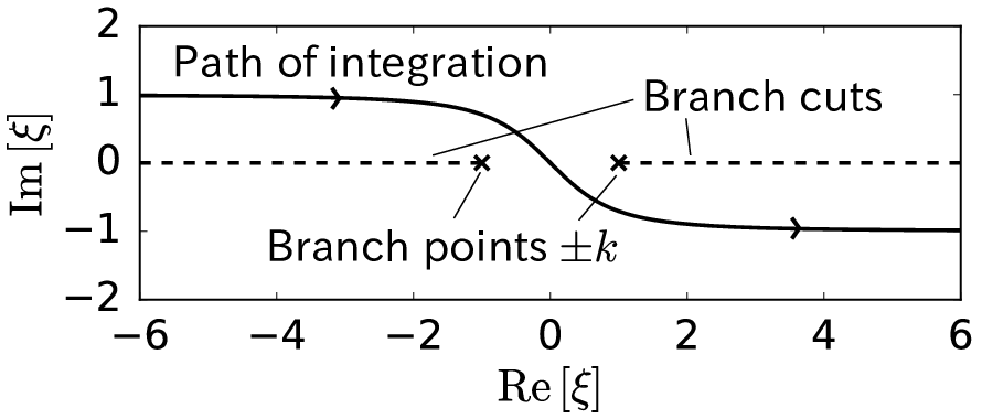
where the integer is arbitrary. This integral representation is a modified version of Linton’s integral form linton2006schlomilch. To obtain the convergence of the integral in eq. 29, we have to determine the branch cuts of the integrand, choose an appropriate sheet, and deform the integration path to circumvent the branch cuts. A possible choice is , where is the principal argument. Here, we can choose a path of integration as the steepest descent path of to obtain a rapid convergence. Thus, we use the path given by for , where . fig. 4 illustrates the path of integration and branch cuts from which we confirm that the path does not cross the branch cuts. Finally, we obtain
| (32) |
Because the integrand in eq. 32 is oscillatory and has a weak singularity of order at , we further apply the double-exponential formula ooura1999robust to this integral in the practical computation.
Although the integral expression eq. 29 is originally proposed for real and , the convergence of the Fourier integral eq. 32 is still achieved for complex and . To see this, let us evaluate the integrand in eq. 32 as follows:
| (33) |
This estimation shows that the integral eq. 32 is convergent even if or . The representation eq. 32 has an infinite number of branch points at for , yielding the Rayleigh anomaly. More careful investigations nose2014calculation show that all branch cuts of for a fixed are written as and .

In fig. 5, we plot the values of calculated using the lattice sum eq. 28 and integral representation eq. 32 with to validate the expressions. The lattice sum eq. 28 is truncated at . In this computation, the comparison between eq. 28 and eq. 32 is given only along the real axis because the lattice sum eq. 28 is divergent otherwise. The results show that is smoothly extended into the complex -plane except for the branch cuts. In addition, the values are in good agreement with the truncated lattice sum.
2.5 Modal analysis
The scattering-matrix formalism eq. 27 allows us to perform guided- and leaky-mode analysis by finding pairs such that the linear system eq. 27 has a nontrivial solution without any incident field . This is a nonlinear eigenvalue problem for the matrix-valued function when either or is fixed in . Therefore, it can be solved using a gradient- or contour integral-based algorithm. In this study, we adopt the Sakurai–Sugiura method (SSM) asakura2009numerical, which determines an eigenpair of , where denotes a matrix-valued and possibly nonlinear function, within a closed path in by integrating for some and on and converting the nonlinear eigenvalue problem into a generalized eigenvalue problem. The SSM can find multiple eigenvalues (even if they are degenerated) in when an appropriate parameter is given in the algorithm. This approach is originally proposed and validated by Nose and Nishimura nose2014calculation with a fast multipole method. They applied the SSM to find nonlinear eigenvalues of a coefficient matrix that arises in a BEM with quasi-periodic Green’s function. We refer to asakura2009numerical for more details about the SSM algorithm.
For a fixed , a guided mode propagates along periodic obstacles without attenuation in space, meaning that a resonant wavenumber is real. On the other hand, if is complex, the corresponding mode decays exponentially as it travels along the structure. In this case, we say that a resonant mode is leaky. A leaky mode satisfies the original boundary value problem eqs. 1, 2, 3, 4 and 5. Furthermore, if the pair and lies in the radiation continuum, i.e., for some , then the bound state is called a BIC.
3 Topology optimization
In this section, we design the shape and topology of a unit structure comprising a periodic waveguide such that it exhibits desirable resonant properties. To this end, we use a topology optimization approach bendsoe2013topology to seek an optimal material distribution for a given objective functional. Here, the objective functional is set as with a resonant wavenumber . To apply topology optimization, we need a sensitivity of the given objective functional with respect to a geometrical perturbation, called a topological derivative. In this section, we first derive a novel expression of the topological derivative for the eigenvalue problem in section 3.1 and then explain the algorithm for the topology optimization in section 3.2.
3.1 Topological derivative
For an effective optimization algorithm, we need sensitivity with respect to a small perturbation of the geometry of a unit structure. In this subsection, we derive topological derivatives sokolowski1999topological related to resonant properties of the periodic waveguide.
3.1.1 Scattering matrix

Here, we first investigate the perturbation of the scattering matrix associated with a single scatterer by a small particle added at a point in either or . Let be an open disk of radius centered at . First, we consider the case of and assume that the disk is characterized by and , i.e. comprises the same material filling in , as shown in fig. 6 (a). For sufficiently small radius , let denote the perturbation of , i.e.
| (34) |
Recall that the scattering matrix is given by
| (35) |
which yields the variation
| (36) |
where denotes the solution of the boundary value problem eqs. 1, 2, 3, 4 and 5 for , and represents the solution of the boundary value problem defined by replacing with in eqs. 1, 2, 3, 4 and 5.
Let be an adjoint variable satisfying the Helmholtz equations
| (37) | ||||
| (38) |
and the Sommerfeld radiation condition. Then, the reciprocity theorem yields
| (39) | |||
| (40) |
| (41) |
Imposing the boundary conditions
| (42) | |||
| (43) |
eq. 41 is reduced to . Substituting this into eq. 36, we obtain
| (44) |
Here, we have used the reciprocity . From the boundary conditions eqs. 42 and 43, we have . This formula further simplifies eq. 44 as follows:
| (45) |
We can no longer simplify the expression eq. 45. However, we are only interested in the asymptotic behavior of for . This can be achieved by expanding with respect to around the point . According to nakamoto2017levelsetbased, we have
| (46) |
Now, we define a topological derivative of , denoted by , as
| (47) |
where denotes the variation of due to the topological change. Then, eq. 46 gives the final expression for the topological derivative as follows:
| (48) |
We can treat the case of (fig. 6 (b)) in the same manner. In this case, the topological derivative is given by
| (49) |
3.1.2 Resonant wavenumber
The topological perturbation changes the distribution of the resonant frequencies and wavenumbers of the periodic system, characterized by the equation eq. 27 with . We fix and investigate the variation in caused by the topological change.
Suppose that the equation
| (50) |
and its perturbed system
| (51) |
have nontrivial solutions. We evaluate the difference . From eqs. 50 and 51, we have
| (52) |
Let be a left eigenvector satisfying . Then, multiplying both sides of eq. 52 by , we have
| (53) |
which gives the topological derivative
| (54) |
Here, we have neglected the higher-order variations.
3.2 Algorithm for the topology optimization

Herein, we perform the topology optimization to find a shape of a unit structure that minimizes the objective functional for a fixed . If the objective value attains , the obtained shape should exhibit a BIC at the target frequency. To this end, we employ a level-set-based topology optimization algorithm.. First, we define a scalar function , called a level-set function, within a fixed design domain . The level-set function gives the material distribution in by
| (55) | |||
| (56) | |||
| (57) |
Instead of seeking an optimal shape of directly, level-set-based topology optimization methods optimize the distribution of using iterative algorithms. This procedure is illustrated in fig. 7. Following amstutz2006new, we iteratively update the level-set function by the following formula:
| (58) |
where denotes the level-set function at th step, denotes a step length, represents the topological derivative of the objective functional corresponding to at th step, and denotes the inner product in defined by
| (59) |
for scalar functions and in . In the iterative algorithm, the functions and are discretized using the B-spline basis functions isakari2017topology. Once the iterative procedure eq. 58 reaches convergence, we terminate the algorithm and obtain the optimal shape of corresponding to .
4 Numerical examples
In this section, we first verify the proposed method and examine the correctness of the new topological derivative. Subsequently, we present a numerical example of the topology optimization that designs a resonant waveguide exhibiting a BIC at a given frequency.
4.1 Verification of the scattering matrix method

First, we verify that the proposed method determines a BIC accurately. As shown in fig. 8, we consider a waveguide comprising circular elastic materials of radius with mass density and bulk modulus embedded in the background medium characterized by and . According to nose2014calculation, this waveguide has a complex eigenvalue for .

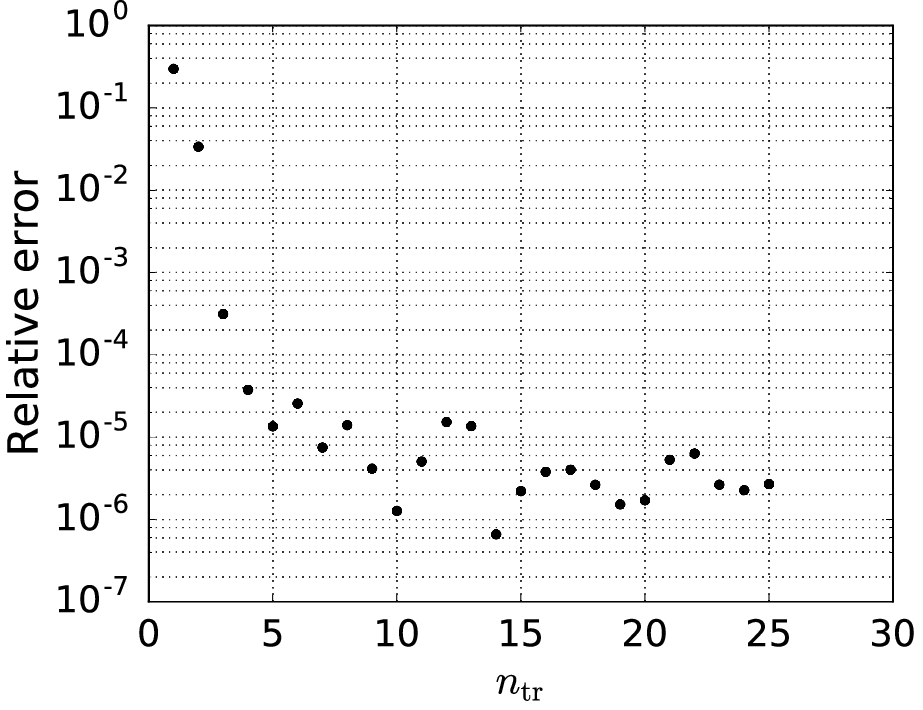
We employ the SSM for a circular contour path of radius centered at in the complex -plane to determine the eigenvalue. The SSM algorithm performs contour integration along using the trapezoidal rule with 32 subintervals. Note that the path does not cross any branch cut for . We discretize a unit disk in fig. 8 using piecewise constant boundary elements. The number of boundary elements is denoted by .
First, we perform the eigenvalue analysis for each (), where is defined as , and fixed . fig. 9 (a) shows the relative error of a unique eigenvalue inside defined by for each . The result shows that the relative error decreases monotonically and converges at the rate of . For , the obtained eigenvalue is , which is close to the value reported in nose2014calculation. Further, we fix at and define a relative error in an analogous manner for . fig. 9 (b) shows the result of the error analysis. The result of the error analysis shows that the error monotonically decreases until it reaches around , which is close to the value at in fig. 9 (a). From these convergence tests, we conclude that the proposed method can determine resonant wavenumbers correctly.
4.2 Topological derivative
In this section, we examine the correctness of the topological derivative formulated in Section 3.1 through a numerical experiment.
In this experiment, we use the same parameters and configuration as those used in the previous example. We compare the derivative with the finite difference for some center and small radius to verify the topological derivative.


First, we fix the center at and investigate an appropriate radius . Figure 10 (a) illustrates the behavior of the finite difference approximation of with respect to the radius . The result shows that the approximation almost converges at and oscillates for smaller due to the loss of significant digits in computing the numerator. Thus, we can expect that produces a reasonable approximation to the topological derivative.
Then, we use and compare the approximation and topological derivative. Figure 10 (b) shows the approximation and derivative along the line , illustrating that both values are consistent. Therefore, we conclude that the proposed topological derivative is accurate.
4.3 Band calculation

In the previous experiments, we have focused on a single resonant wavenumber. However, we are often interested in how the eigenvalue depends on the frequency, i.e., phononic band structure. Because of the quasiperiodicity and time-reversal symmetry, it suffices to find eigenvalues in for a fixed . In the following numerical experiment, we set a path of integration for the SSM algorithm (fig. 11) with .

Figure 12 (a) shows the plot of the band structure obtained using the proposed method. In the diagram, the computed eigenvalues are replaced with , where is an integer that satisfies . The obtained band diagram has some similar features to that of planar waveguides hu2009understanding. For example, the diagram (fig. 12 (a)) shows that the third band departs from the lightline at around (cutoff frequency). In addition, the first band satisfies . They are typical characteristics of the waveguide dispersion. The figure shows that the eigenvalues outside the radiation continuum, which is the region below the lightlines, have small imaginary parts, thus forming guided modes along the periodic structure. Within the radiation continuum (gray-shaded region in fig. 12 (a)), almost every eigenmode is leaky due to its nonzero imaginary part. However, we find a significantly small imaginary part within the continuum around and . fig. 12 (b) shows that the absolute values of the imaginary part decrease rapidly around and , indicating that two BICs exist around the points. The latter point stands for a symmetry-protected BIC hsu2016bound because it lies on the point (). As long as the parity symmetry with respect to is preserved and the material parameters satisfy a certain condition, there exists at least one symmetry-protected BIC with bonnet-bendhia1994guided, shipman2010resonant. Further, we conducted an eigenvalue analysis to find a resonant for fixed . We obtained that is an eigenpair, whose mode profile is illustrated in fig. 12 (c). fig. 12 (d) shows the resonant mode corresponding to . From the mode profiles, we observe that the fields are strongly confined around the structure without radiation. This type of BICs on the second band with are already reported and discussed for circular inclusions bulgakov2014bloch, yuan2018bound.
4.4 Topology optimization
From the previous subsection, we observed that the periodic array of circular cylinders exhibits some BICs. Although only the two BICs are found in the band diagram, the existence of BICs in a higher frequency regime is reported for a simple geometry bonnet-bendhia1994guided. In this section, we show that the topology optimization can realize a new BIC for a given higher frequency.
We use the same material parameters as previous experiments. Using the topology optimization, we minimize the imaginary part of the resonant wavenumber at of the periodic structure shown in fig. 8. To this end, we set the objective functional as and determine an optimized unit structure within the fixed design domain , so that it exhibits a BIC if attains the value of zero. The size of the fixed design domain is chosen to avoid violating the well-separated condition (described in Section 2.3).


figs. 13 and 14 show the results of the topology optimization. We obtain the optimized shape shown in fig. 13 using the topology optimization for the unit structure. This structure has a resonant wavenumber of (corresponding to the objective value ) at . fig. 14 (b) shows the convergence history of . The figure shows that the topology optimization successfully decreases the value of . We also conduct a band analysis for the optimized shape and plot the band structure in fig. 14 (a). From the band structure, we observe that the optimized shape has small imaginary parts around , whereas the initial shape has relatively large imaginary parts (fig. 12 (a)). Although the obtained eigenvalue has a significantly small imaginary part, we cannot guarantee that this is a true BIC because of numerical errors that arise in the BEM and SSM.

To show that the optimized structure supports a guided wave at the desired frequency , we investigate the scattering of the cylindrical wave through the optimized array with source point (fig. 15). We compute the energy fluxes and across the lines and , respectively. fig. 15 (b) shows the plot of the transmittance and frequency. The figure shows that the spectrum has peaks at and , corresponding to the eigenvalues with small imaginary parts in fig. 14 (a). Figure 15 (c) and (d) show the total field when the incident wave illuminates the array for and , respectively. We also plot the real part of the total field at in Figure 15 (e); it shows the similar wave profile to the new BIC (fig. 14 (c)). These results show that the incident field excites the guided mode (BIC) at realized by the topology optimization; however, it exhibits no coupling to any guided mode for .

We can also observe a BIC by finding Wood’s anomaly in a scattering analysis Monticone2017bound. As shown in fig. 16 (a), we analyze the scattering of a plane wave by the optimized structure. The incident angle is given by so that the line crosses the band at as shown in fig. 16 (b). Figure 16 (c) shows the reflectance, which is defined by the downward energy flux divided by the incident energy flux per unit cell, versus the angular frequency. The spectrum exhibits a sharp resonance at , corresponding to the BIC realized through the topology optimization. Further analyses show that a solution of the scattering problem is not unique at exact BICs bonnet-bendhia1994guided, shipman2010resonant.

In the band diagram shown in fig. 14 (a), the optimized BIC occurs at the crossing of two bands. To check whether this is a necessary condition for realizing a BIC, we conduct the same topology optimization at the frequency with resonant wavenumber in the initial diagram, shown in fig. 12 (a). The optimized geometry and diagram are plotted in fig. 17. The results show that the obtained BIC with is not a crossing point in the diagram, meaning that the crossing is not a necessary condition.
5 Conclusions
This study proposed a topology optimization scheme for designing resonant waveguides exhibiting BICs at desired frequencies in the two-dimensional space. We formulated the periodic problem using the scattering matrix of a unit structure and computed resonant wavenumbers using the BEM and SSM. Moreover, we derived a topological derivative of resonant wavenumbers. In the numerical experiments, we first demonstrated that the proposed method determines a resonant wavenumber accurately. Subsequently, we performed a topology optimization to realize a new BIC at a given frequency. Although we considered Helmholtz’ equation for a singly periodic system in two dimensions, the underlying idea, which is the combination of BEM, SSM, and topology optimization, would be applicable to two-dimensional problems and other wave fields governed by Maxwell’s equations or elastodynamics.
Acknowledgements
The authors would like to acknowledge anonymous referees for their valuable comments. This work was supported by JSPS KAKENHI Grant Numbers JP19J21766 and JP19H00740.
References
- [1] C. W. Hsu, B. Zhen, A. D. Stone, J. D. Joannopoulos, M. Soljačić, Bound states in the continuum, Nature Reviews Materials 1 (9) (2016) 1–13. doi:10.1038/natrevmats.2016.48.
- [2] J. von Neumann, E. P. Wigner, über merkwürdige diskrete Eigenwerte, Physikalische Zeitschrift 30 (1929) 465–467.
- [3] Y. Plotnik, O. Peleg, F. Dreisow, M. Heinrich, S. Nolte, A. Szameit, M. Segev, Experimental observation of optical bound states in the continuum, Physical Review Letters 107 (18) (2011) 183901. doi:10.1103/PhysRevLett.107.183901.
- [4] J. Lee, B. Zhen, S.-L. Chua, W. Qiu, J. D. Joannopoulos, M. Soljačić, O. Shapira, Observation and differentiation of unique high- optical resonances near zero wave vector in macroscopic photonic crystal slabs, Physical Review Letters 109 (6) (2012) 067401. doi:10.1103/PhysRevLett.109.067401.
- [5] C. W. Hsu, B. Zhen, J. Lee, S.-L. Chua, S. G. Johnson, J. D. Joannopoulos, M. Soljačić, Observation of trapped light within the radiation continuum, Nature 499 (7457) (2013) 188–191. doi:10.1038/nature12289.
- [6] C. M. Linton, P. McIver, Embedded trapped modes in water waves and acoustics, Wave Motion 45 (1) (2007) 16–29. doi:10.1016/j.wavemoti.2007.04.009.
- [7] F. Dreisow, A. Szameit, M. Heinrich, R. Keil, S. Nolte, A. Tünnermann, S. Longhi, Adiabatic transfer of light via a continuum in optical waveguides, Optics Letters 34 (16) (2009) 2405–2407. doi:10.1364/OL.34.002405.
- [8] Y. Yang, C. Peng, Y. Liang, Z. Li, S. Noda, Analytical perspective for bound states in the continuum in photonic crystal slabs, Physical Review Letters 113 (3) (2014) 037401. doi:10.1103/PhysRevLett.113.037401.
- [9] E. N. Bulgakov, A. F. Sadreev, Bloch bound states in the radiation continuum in a periodic array of dielectric rods, Physical Review A 90 (5) (2014) 053801. doi:10.1103/PhysRevA.90.053801.
- [10] A. Kodigala, T. Lepetit, Q. Gu, B. Bahari, Y. Fainman, B. Kanté, Lasing action from photonic bound states in continuum, Nature 541 (7636) (2017) 196–199. doi:10.1038/nature20799.
- [11] J. M. Foley, S. M. Young, J. D. Phillips, Symmetry-protected mode coupling near normal incidence for narrow-band transmission filtering in a dielectric grating, Physical Review B 89 (16) (2014) 165111. doi:10.1103/PhysRevB.89.165111.
- [12] A. A. Yanik, A. E. Cetin, M. Huang, A. Artar, S. H. Mousavi, A. Khanikaev, J. H. Connor, G. Shvets, Hatice Altug, Seeing protein monolayers with naked eye through plasmonic Fano resonances, Proceedings of the National Academy of Sciences 108 (29) (2011) 11784–11789. doi:10.1073/pnas.1101910108.
- [13] J. Sokolowski, J.-P. Zolesio, Introduction to Shape Optimization: Shape Sensitivity Analysis, Springer Series in Computational Mathematics, Springer, Berlin, Heidelberg, 1992.
- [14] M. P. Bendsøe, O. Sigmund, Topology Optimization: Theory, Methods, and Applications, Springer Science & Business Media, 2013.
- [15] D. C. Dobson, S. J. Cox, Maximizing band gaps in two-dimensional photonic crystals, SIAM Journal on Applied Mathematics 59 (6) (1999) 2108–2120. doi:10.1137/S0036139998338455.
- [16] D. Evans, R. Porter, Trapped modes embedded in the continuous spectrum, Quarterly Journal of Mechanics and Applied Mathematics 51 (2) (1998) 263–274. doi:10.1093/qjmam/51.2.263.
- [17] R. Porter, D. V. Evans, Embedded Rayleigh–Bloch surface waves along periodic rectangular arrays, Wave Motion 43 (1) (2005) 29–50. doi:10.1016/j.wavemoti.2005.05.005.
- [18] L. G. Bennetts, M. A. Peter, Rayleigh–Bloch waves above the cutoff, Journal of Fluid Mechanics 940. doi:10.1017/jfm.2022.247.
- [19] J. Hu, C. R. Menyuk, Understanding leaky modes: Slab waveguide revisited, Advances in Optics and Photonics 1 (1) (2009) 58–106. doi:10.1364/AOP.1.000058.
- [20] H. Ammari, A. Dabrowski, B. Fitzpatrick, P. Millien, Perturbation of the scattering resonances of an open cavity by small particles. Part I: The transverse magnetic polarization case, Zeitschrift für angewandte Mathematik und Physik 71 (4) (2020) 102. doi:10.1007/s00033-020-01324-6.
- [21] Z. Gimbutas, L. Greengard, Fast multi-particle scattering: A hybrid solver for the Maxwell equations in microstructured materials, Journal of Computational Physics 232 (1) (2013) 22–32. doi:10.1016/j.jcp.2012.01.041.
- [22] J. Sokolowski, A. Zochowski, On the topological derivative in shape optimization, SIAM Journal on Control and Optimization 37 (4) (1999) 1251–1272. doi:10.1137/S0363012997323230.
- [23] H. Isakari, T. Takahashi, T. Matsumoto, A topology optimisation with level-sets of B-spline surface (in Japanese), Transactions of the Japan Society for Computational Methods in Engineering 17 (2017) 125–130.
- [24] A. J. Burton, G. F. Miller, J. H. Wilkinson, The application of integral equation methods to the numerical solution of some exterior boundary-value problems, Proceedings of the Royal Society of London. A. Mathematical and Physical Sciences 323 (1553) (1971) 201–210. doi:10.1098/rspa.1971.0097.
- [25] C.-J. Zheng, H.-B. Chen, H.-F. Gao, L. Du, Is the Burton–Miller formulation really free of fictitious eigenfrequencies?, Engineering Analysis with Boundary Elements 59 (2015) 43–51. doi:10.1016/j.enganabound.2015.04.014.
- [26] M. Abramowitz, I. A. Stegun, Handbook of Mathematical Functions with Formulas, Graphs, and Mathematical Tables, Dover Publications, 1965.
- [27] P. A. Martin, Multiple Scattering: Interaction of Time-harmonic Waves with N Obstacles, Cambridge University Press, 2006.
- [28] R. Coifman, V. Rokhlin, S. Wandzura, The fast multipole method for the wave equation: A pedestrian prescription, IEEE Antennas and Propagation Magazine 35 (3) (1993) 7–12. doi:10.1109/74.250128.
- [29] N. A. Nicorovici, R. C. McPhedran, L. C. Botten, Photonic band gaps for arrays of perfectly conducting cylinders, Physical Review E 52 (1) (1995) 1135–1145. doi:10.1103/PhysRevE.52.1135.
- [30] C. M. Linton, Schlömilch series that arise in diffraction theory and their efficient computation, Journal of Physics A: Mathematical and General 39 (13) (2006) 3325–3339. doi:10.1088/0305-4470/39/13/012.
- [31] R. Porter, D. V. Evans, Rayleigh–Bloch surface waves along periodic gratings and their connection with trapped modes in waveguides, Journal of Fluid Mechanics 386 (1999) 233–258. doi:10.1017/S0022112099004425.
- [32] Y. Otani, N. Nishimura, An FMM for periodic boundary value problems for cracks for Helmholtz’ equation in 2D, International Journal for Numerical Methods in Engineering 73 (3) (2008) 381–406. doi:10.1002/nme.2077.
- [33] H. Isakari, K. Niino, H. Yoshikawa, N. Nishimura, Calderon’s preconditioning for periodic fast multipole method for elastodynamics in 3D, International Journal for Numerical Methods in Engineering 90 (4) (2012) 484–505. doi:10.1002/nme.3332.
- [34] T. Nose, N. Nishimura, Calculation of eigenvalues related to 2 dimensional periodic boundary value problems for the Helmholtz equation using the Sakurai-Sugiura method and periodic fast multipole method (in Japanese), Transactions of the Japan Society for Industrial and Applied Mathematics 24 (2014) 185–201.
- [35] R. Misawa, K. Niino, N. Nishimura, An FMM for waveguide problems of 2-D Helmholtz’ equation and its application to eigenvalue problems, Wave Motion 63 (2016) 1–17. doi:10.1016/j.wavemoti.2015.12.006.
- [36] T. Ooura, M. Mori, A robust double exponential formula for Fourier-type integrals, Journal of Computational and Applied Mathematics 112 (1) (1999) 229–241. doi:10.1016/S0377-0427(99)00223-X.
- [37] J. Asakura, T. Sakurai, H. Tadano, T. Ikegami, K. Kimura, A numerical method for nonlinear eigenvalue problems using contour integrals, JSIAM Letters 1 (2009) 52–55. doi:10.14495/jsiaml.1.52.
- [38] K. Nakamoto, H. Isakari, T. Takahashi, T. Matsumoto, A level-set-based topology optimisation of carpet cloaking devices with the boundary element method, Mechanical Engineering Journal 4 (1) (2017) 16–00268. doi:10.1299/mej.16-00268.
- [39] S. Amstutz, H. Andrä, A new algorithm for topology optimization using a level-set method, Journal of Computational Physics 216 (2) (2006) 573–588. doi:10.1016/j.jcp.2005.12.015.
- [40] A.-S. Bonnet-Bendhia, F. Starling, Guided waves by electromagnetic gratings and non-uniqueness examples for the diffraction problem, Mathematical Methods in the Applied Sciences 17 (5) (1994) 305–338. doi:10.1002/mma.1670170502.
- [41] S. P. Shipman, Resonant scattering by open periodic waveguides, in: Progress in Computational Physics, Vol. 1, Bentham Science Publishers, 2010.
- [42] L. Yuan, Y. Y. Lu, Bound states in the continuum on periodic structures surrounded by strong resonances, Physical Review A 97 (4) (2018) 043828. doi:10.1103/PhysRevA.97.043828.
- [43] F. Monticone, A. Alù, Bound states within the radiation continuum in diffraction gratings and the role of leaky modes, New Journal of Physics 19 (9) (2017) 093011. doi:10.1088/1367-2630/aa849f.