The value-added catalogue for LAMOST DR8 low-resolution spectra
Abstract
We present a value-added catalog containing stellar parameters estimated from 7.10 million low-resolution spectra for 5.16 million unique stars with spectral signal-to-noise ratios (SNRs) higher than 10 obtained by the Large Sky Area Multi-Object Fibre Spectroscopic Telescope (LAMOST) Galactic spectroscopic surveys. The catalog presents values of stellar atmospheric parameters (effective temperature , surface gravity , metallicity [Fe/H]/[M/H]), -element to metal abundance ratio [/M], carbon and nitrogen to iron abundance ratios [C/Fe] and [N/Fe] and 14 bands’ absolute magnitudes deduced from LAMOST spectra using the method of neural network. The spectro-photometric distances of those stars are also provided based on the distance modulus. For stars with spectral SNRs larger than 50, precisions of , , [Fe/H], [M/H], [C/Fe], [N/Fe] and [/M] are 85 K, 0.098 dex, 0.05 dex, 0.05 dex, 0.052 dex, 0.082 dex and 0.027 dex, respectively. The errors of 14 band’s absolute magnitudes are 0.16–0.22 mag for stars with spectral SNRs larger than 50. The spectro-photometric distance is accurate to 8.5% for stars with spectral SNRs larger than 50, and is more accurate than geometrical distance for stars with distance larger than 2.0 kpc. Our estimates of [Fe/H] are reliable down to [Fe/H] dex, significantly better than previous results. The catalog provide 26,868 unique very metal poor star candidates ([Fe/H] ). The catalog would be a valuable data set to study the structure and evolution of the Galaxy, especially the solar-neighbourhood and the outer disc.
I Introduction
As a typical disc galaxy, the Milky Way (MW) is an ideal laboratory to test galaxy formation and evolution scenarios with the advantage that the individual stars in the MW can be well resolved. A number of completed or ongoing large-scale spectroscopic surveys, e.g., RAVE (Steinmetz et al. 2006), SEGUE (Yanny et al. 2009), LAMOST Experiment for Galactic Understanding and Exploration (Deng et al. 2012; Liu et al. 2014; Zhao et al. 2012, LEGUE; ), Gaia-ESO (Gilmore et al. 2012), Galactic Archaeology with HERMES (De Silva et al. 2015, GALAH; ), Apache Point Observatory Galactic Evolution Experiment (Majewski et al. 2017, APOGEE; ), Gaia Radial Velocity Spectrometer (Cropper et al. 2018), and the MMT H3 survey (Conroy et al. 2019) — as well as the upcoming surveys such as SDSS-V (Kollmeier et al. 2017), 4MOST (Feltzing et al. 2018; de Jong et al. 2019), and WEAVE (Dalton et al. 2014), have propelled studies of the structure, stellar populations and the chemical and dynamic evolution of the MW. Stellar atmospheric parameters and elemental abundances of stars could be accurately derived from high-to-low resolution spectra collected by those massive spectroscopic surveys. Those rich information from spectroscopic surveys, together with the accurate parallax and proper motions from the Gaia missions (Gaia Collaboration et al. 2016; Gaia Collaboration et al. 2018; Gaia Collaboration et al. 2020), will significantly advance our knowledge of the formation and evolution of our Galaxy.
The LAMOST Galactic survey (Deng et al. 2012; Liu et al. 2014; Zhao et al. 2012) is the first spectroscopic survey to obtain spectra of 10 million stars. For the LAMOST spectra, several efforts have been made to derive the radial velocities , stellar atmospheric parameters (effective temperature , surface gravity , metallicity ), individual element abundances, distance and extinctions (Yuan et al. 2015; Luo et al. 2015; Xiang et al. 2015a; Xiang et al. 2017). The official LAMOST Stellar parameter Pipeline (Luo et al. 2015, LASP; ) and the LAMOST Stellar Parameter Pipeline at Peking University (Xiang et al. 2015a; Xiang et al. 2017, LSP3; ) have been developed to estimate the radial velocities and atmospheric parameters from LAMOST spectra for A/F/G/K-type stars, with typical uncertainties of , , and , respectively, of 100–200 K, 0.1–0.3 dex, 0.1–0.2 dex and 5 (Gao et al. 2015; Luo et al. 2015; Ren et al. 2016; Xiang et al. 2015a; Xiang et al. 2017; Wang et al. 2016; Huang et al. 2018) for FGK type stars with spectral SNR . -element to iron abundance ratio [/Fe] and abundances of individual elements (C, N, O, Na, Mg, Al, Si, Ca, Ti, Cr, Mn, Fe, Co, Ni, Cu, and Ba) are also derived (Li et al. 2016; Xiang et al. 2017; Xiang et al. 2019; Ting et al. 2017), for SNR 50, their uncertainties are 0.03–0.1 dex except Cu and Ba (with uncertainties of 0.2–0.3 dex). In addition, some other efforts have been made to derive stellar parameters from LAMOST spectra, e.g., the Stellar LAbel Machine (Zhang et al. 2020, SLAM; ), the analysis based on SP_Ace code (Boeche et al. 2018), the stellar parameter determinations based on the (Ho et al. 2017), an application of the SEGUE Stellar Parameter Pipeline (SSPP) to LAMOST spectra (Lee et al. 2015) and the hotPayne from deriving stellar labels for hot, OBA stars (Xiang et al. 2021b). Value-added catalogs of stellar parameters from these efforts have been widely utilized for unraveling structure and evolution of our Galaxy (Huang et al. 2015; Sun et al. 2015; Xiang et al. 2015b; Chen et al. 2016; Huang et al. 2016; Liu et al. 2017; Xiang et al. 2018; Xu et al. 2018; Huang et al. 2019; Kamdar et al. 2019; Gandhi & Ness 2019; Li et al. 2019; Wang et al. 2019a; Wang et al. 2019b; Sharma et al. 2021a; Sharma et al. 2021b; Vickers et al. 2021, e.g.,).
Due to the lack of very metal-poor stars (VMP; [Fe/H] ) as the spectral templates or training samples, the stellar labels are generally less well estimated for very metal-poor stars with [Fe/H] . The [Fe/H] values of VMP stars need to be estimated separately by special considerations (Li et al. 2018). The PASTEL (Soubiran et al. 2010) catalog provides accurate stellar atmospheric parameters including , and [Fe/H]. Moreover, the PASTEL catalog contains tens of VMP stars (in common with LAMOST) with accurate stellar atmospheric parameters, which can be adopted as the training set for LAMOST to estimate the stellar atmospheric parameters, especially the metallicity values of VMP stars. For the estimates of [/Fe] and individual elemental abundance [X/H] from LAMOST low-resolution spectra, previous works mostly use the APOGEE DR15/DR14 or GALAH as training set for giant and dwarf stars. Compared with APOGEE DR15/DR14, the APOGEE DR16 provides more precise measurements of metallicity [Fe/H], -element to metal/iron abundance ratio [/Fe]/[/M], individual elemental abundance [X/H] and individual elemental abundance to iron ratios [X/Fe], especially for dwarf stars. Adopting the APOGEE DR16 as training set, we could obtain good estimates of individual elemental abundances for both giant and dwarf stars.
The absolute magnitudes present the luminosity of stars and thus are useful for estimating the distances and ages of stars, which are indispensable when we study the structures and chemo-dynamical evolutions of our Galaxy. The early Gaia DR3 (Gaia Collaboration et al. 2020, hereafter EDR3;) have provided parallaxes, proper motions of 1.8 billion Galactic stars. The geometrical distances (Bailer-Jones et al. 2021) of 1.47 billion stars in the Milky Way have also been provided. Within 2 kpc from the Sun, the geometrical distance is accurate to 10 per cent. The uncertainties and systematic errors of geometrical distance become larger for distant stars, especially those beyond 2 kpc. For those stars far from ( kpc) the Sun, the spectro-photometric distance is a better choice, as it is less distance-dependent and may provide better precision (Xiang et al. 2017; Xiang et al. 2021a, e.g., ). The common stars of LAMOST, Gaia EDR3 and other photometric surveys provide a good training set to estimate absolute magnitudes from spectra directly for deriving the sepctro-photometric distances for all stars with LAMOST low-resolution spectra.
By March 2021, Low-Resolution Spectroscopic Survey of LAMOST DR8 have released 11,212,561 optical (3700–9000 Å) spectra with a resolution of 1800, of which more than 90 per cent are stellar spectra. The classifications, radial velocity and stellar atmospheric parameters for those spectra are provided by LAMOST DR8.
In this work, we present a value-added catalog for LAMOST DR8 low-resolution spectra. The catalog provide stellar atmospheric parameters (, , /[M/H]), absolute magnitudes of 14 different wavelength bands adopted by different photometric surveys ( of Gaia EDR3, of 2MASS, of WISE, of APASS and of SDSS), elemental abundances to metal or iron ratios ([/M], [C/Fe], [N/Fe]) and spectro-photometric distances for stars targeted by LAMOST with their low-resolution spectra in LAMOST DR8. We firstly exploite a machine learning method based on neural network (NN) to estimate effective temperature, surface gravity, metallicity, absolute magnitudes, and individual elemental abundances from the LAMOST DR8 low-resolution spectra, utilizing the aforementioned spectral training sets. The distances of those stars are then estimated using the apparent magnitudes, extinctions and our estimated absolute magnitudes.
The paper is organized as follows. Section 2 introduces the used neural network method and models. Section 3 presents the training sets. In Section 4, we present the estimates of stellar parameters derived from LAMOST spectra using neural network method, including a detailed error analysis. We present the improved metallicity estimates of very metal poor stars in Section 5. In Section 6, we introduce the estimates of spectro-photometric distance. We discuss the nature of the final value-added catalog and present a perspective of the catalog on the future in Section 7, followed by a summary in Section 8.
II The neural network method and models
, , and other chemical elemental abundances are stellar parameters that can be derived from stellar spectra. As discussed by Xiang et al. 2020, the luminosity (absolute magnitude) of a star is related to the effective temperature, mass and surface gravity of the star according to the Stefan-Boltzmann equation and gravity equation. The stellar mass also implicitly depends on , , and stellar rotation. Thus, the luminosity (absolute magnitude) could be directly derived from stellar spectra. In this section, we introduce neural network method and models, which model the empirical relation between the LAMOST spectra and , , , [M/H], [/M], [C/Fe], [N/Fe] and absolute magnitudes of 14 photometric bands aforementioned using different training sets.
II.1 The neural network models
To build up a relation between spectra and effective temperature, surface gravity, element abundances and absolute magnitudes of stars, we adopt a feed-forward multi-layer perceptron neural network model, which is similar to that of Ting et al. 2017; Ting et al. 2019 and Xiang et al. 2020; Xiang et al. 2021a. Adopting the Einstein sum notation, our neural network contains three-layers and can be succinctly written as:
| (1) |
where is the stellar atmospheric parameters, element abundances or absolute magnitudes of stars; is the Relu activation function; and are weights and biases of the network to be optimized; the index , and denotes the number of neurons in the third, second and first layer; and denotes the wavelength pixel. The total number of neurons for first, second and third layer are respectively 512, 256 and 64. The training process is carried out with the package in .
II.2 Pre-processing for the spectra
The LAMOST spectra cover a wavelength range of 3700–9000. However, we only use 3900-5800 Å and 8450–8950 Å to determine the effective temperature, surface gravity, element abundance ratios and absolute magnitudes of stars. First the SNR of very blue part (3700–3900 Å) of the spectra is quite low for most of stars. Secondly, the spectra of 5800–8450 Å suffer from serious background contamination (including sky emission lines and telluric bands). Besides, the effective information in spectra of 5800–8450 Å is very limited.
Because of the unknown extinction values for most of the survey targets and the relatively large uncertainties of spectral flux calibration of LAMOST spectra, it is better to use continuum-normalized spectra to deliver reliable stellar parameters (Xiang et al. 2017, e.g.,). All LAMOST stellar spectra are normalized by dividing their pseudo-continuum spectra. Each pseudo-continuum spectrum is derived through using a sixth-order polynomial to fit the smoothed spectra of wavelength 3900-5800 Å and 8450–8950 Å , separately. The smoothed spectra are obtained via median filtering method with a filter size of 21 pixels.
For neural-network method, to avoid the issues due to the different scales in different dimensions of the input data, all the normalized spectral fluxes and the stellar labels of the training sets should be normalized in a standard space (with zero mean and unity variance). All LAMOST normalized spectra are also normalized in standard space with the same scale of training sets.
III The training sets
In the current work, we define three training sets to estimate stellar paramters: the LAMOST–PASTEL common stars, the LAMOST–APOGEE common stars and the LAMOST–Gaia EDR3–2MASS–WISE–APASS–SDSS (hereafter referred to as “the LGMWAS”) common stars. The LAMOST–PASTEL common stars are used to estimate effective temperature , surface gravity and metallicity . The LAMOST–APOGEE common stars are used to estimate the , [Fe/H], [M/H], [/M], [C/Fe] and [N/Fe]. Note that here we will give two and [Fe/H] values for each low-resolution spectra in LAMOST DR8, which are estimated using LAMOST–PASTEL common stars and LAMOST–APOGEE common stars as training sets, respectively. The LGMWAS common stars are used to estimate absolute magnitudes ( of Gaia EDR3 bands, of 2MASS bands, of WISE bands, of APASS bands, of SDSS bands). Tabel 1 presents the three adopted training sets and their effective parameter ranges.
| Training sets | Parameters | Number of stars | Effective parameter range |
|---|---|---|---|
| K | |||
| LAMOST–PASTEL | , , [Fe/H] | 1,281 | |
| K | |||
| LAMOST–APOGEE | , [Fe/H], [M/H], [/M], [C/Fe], [N/Fe] | 8,753 | |
| LGMWAS | , , , , | 6,000 | |
III.1 The LAMOST–PASTEL common stars
PASTEL is a catalog of bibliographical compilation of accurate stellar atmospheric parameters, including , and [Fe/H], mostly determined from high resolution, high SNR spectra. By 2020, the catalog contains 81,362 stellar atmospheric parameter measurements for more than 31,000 unique stars, collected from more than 11,000 bibliographical references (Soubiran et al. 2016; Soubiran et al. 2020). However, stellar atmospheric parameters coming from different bibliographical references do not have the same scales. Not all of them are mutually independent, systematic deviations among different bibliographic sources may exist because of the different approaches of measuring stellar atmospheric parameters. Besides, not all values of effective temperature and surface gravity listed in PASTEL were determined with high resolution spectra. To solve those problems in PASTEL, we have recalibrated the measurements of stellar atmospheric parameters collected in PASTEL from a variety of sources such that they are on the same scale. The results will be presented in a separate paper (Huang et al. 2021, in preparation).
We find 1,859 common unique stars with good stellar atmospheric parameter determinations through a cross-match between recalibrated PASTEL and LAMOST DR8. Amongst them, 1,743 unique stars have good LAMOST spectra (without bad pixels in the adopted wavelength range, check via eyes), 1,281 unique stars have high quality LAMOST spectra with spectral SNR 50. These 1,281 unique stars are finally adopted as training set. Other 462 uniqe stars are adopted as test set. Fig. 1 shows the distributions of the 1,281 LAMOST–PASTEL training stars in the – and –[Fe/H] planes. With this training set, we estimate the , and [Fe/H]. The training set has a wide coverage of stellar atmospheric parameters: K, dex and [Fe/H] dex.
With the LAMOST–PASTEL training set, we apply neural-network models to construct the relations between the LAMOST spectra and the stellar atmospheric parameters. We use the neural-network models to estimate , and [Fe/H] for LAMOST–PASTEL training and test sets. The estimated , and [Fe/H] could match well with that provided by the PASTEL catalog. The standard deviations of their differences are 75 K for , 0.09 dex for and 0.05 dex for [Fe/H] for the training set, 156 K for , 0.29 dex for and 0.15 dex for [Fe/H] for the test set. The standard deviations of test set are much larger than that of training set. This may be the consequence of that the test sample has lower LAMOST spectral SNRs ( SNR ) and much less stellar members compared to the training sample. The systematic differences between stellar atmospheric parameters coming from PASTEL and the stellar atmospheric parameters derived from LAMOST spectra are very small with 10 K, 0.01 dex and 0.01 dex for both training and test sets. One can see Fig. A1 in Appendix for more details.
It is surprising that the [Fe/H] values derived from LAMOST spectra has no obvious systematic errors down to [Fe/H] (Fig. A1 in Appendix) through comparing with that of PASTEL, which is a big improvement for [Fe/H] determinations from LAMOST low-resolution spectra. It is important for us to build up catalog of VMP stars and carry out follow-up observations of those VMP stars found from the LAMOST.
III.2 The LAMOST–APOGEE common stars
APOGEE DR16 (Jönsson et al. 2020) contains 473,307 high-resolution ( 22,500), multiplexed, near-infrared (15140–16940 Å) spectra for about 437,445 unique stars covering both the northern and southern sky. These spectra are collected using the APOGEE-N (north) instrument (Wilson et al. 2019) in combination with the 2.5 m Sloan Foundation telescope (Gunn et al. 2006) at Apache Point Observatory (APO) in New Mexico and the APOGEE-S (south) with the 2.5 m du Pont telescope (Bowen & Vaughan 1973) at Las Campanas Observatory in Chile (“LCO 2.5 m”). Adopting these spectra, Jönsson et al. 2020 estimate accurate stellar atmospheric parameters (, and [Fe/H]/[M/H]), -element to metal abundance ratio [/M], individual elemental (C, C i, N, O, Na, Mg, Al, Si, P, S, K, Ca, Ti, Ti ii, V, Cr, Mn, Fe, Co, Ni, Cu, Ge, Rb, Ce, Nd, and Yb) abundance ratios [X/H], and carbon and nitrogen to iron ratios [C/Fe] and [N/Fe] based on ASPCAP (García Pérez et al. 2016). These stellar atmospheric parameters and these chemical elemental abundances are well estimated and calibrated. The typical uncertainties of , and individual elemental abundance are respectively 98 K, dex and dex, one can see tabel 6, tabel 7 and tabel 8 of Jönsson et al. 2020 for details.
In this work, we adopt the APOGEE DR16 as the training set to estimate the , [Fe/H], [M/H], [/M], [C/Fe] and [N/Fe]. As discussed in Section 2, we use the LAMOST spectra of 3900-5800 Å and 8450-8950 Å. The selected wavelength range contains spectral features of C, N and -elements (e.g., CN Å, CH 4314Å, Ca i 4226Å and Mg b lines etc.). Theoretically, [/M], [C/Fe] and [N/Fe] could be derived from LAMOST spectra. Previous works (Li et al. 2016; Xiang et al. 2017; Xiang et al. 2019; Ting et al. 2017; Ho et al. 2017; Zhang et al. 2020, e.g.,) have also made efforts to determine the carbon, nitrogen and -element abundance using LAMOST low-resolution spectra and support that even low-resolution spectra could be used to estimate stellar individual element abundances.
A cross-match of LAMOST DR8 with the APOGEE DR16 catalog yields 122,658 stars in common. To derive accurate results, we select stars with the following criteria: . Stars with bad LAMOST spectra are also excluded. Finally, 14,877 stars are selected. We select 8,753 stars as training set, 6,124 stars as test set. In this process, we select as much metal-poor and high [/Fe] stars as possible into training sample in order to construct a better neural network model. Fig. 2 shows the distributions of the LAMOST–APOGEE training stars and test stars in the –, [M/H]–[/M], [M/H]–[C/Fe] and [M/H]–[N/Fe] planes. The training set has a wide coverage of stellar atmospheric parameters: K, dex, [M/H] dex, dex, and .
Note that when we estimate the [C/Fe], we remove stars with . When we estimate the [N/Fe], we remove stars with . The purpose of the cuts is to derive accurate [C/Fe] and [N/Fe].
Using the aforementioned neural network models adopting the LAMOST–APOGEE training stars as training set, the relations between LAMOST spectra and aforementioned stellar parameters are constructed. Then we estimate the [Fe/H], [M/H], [/M], [C/Fe], [N/Fe] and for test stars using these models. The estimated stellar parameters could match well with that provided by APOGEE. The standard deviations of the residuals are only 0.033, 0.032, 0.044, 0.07, 0.018 and 0.067 dex for [Fe/H], [M/H], [C/Fe], [N/Fe], [/M] and , respectively. The systematic differences between APOGEE chemical abundances and chemical abundances derived from LAMOST spectra are very small, almost all of them are smaller than 0.01 dex. The systematic differences between APOGEE and derived from LAMOST spectra is 0.012 dex. One can see Fig. A2 in Appendix for more details about the comparisons between our estimated stellar parameters and those provided by APOGEE DR16.

III.3 The LGMWAS common stars
Gaia EDR3 (Gaia Collaboration et al. 2020) provided precise parallaxes, proper motions and magnitudes of 1.8 billion stars in the MW. Bailer-Jones et al. 2021 estimate the distances and asymmetric uncertainties for 1.47 billion stars by using Gaia EDR3. Within 2 kpc from the Sun, the distance is accurate to 10 per cent. According to the precise distances, apparent magnitudes and interstellar extinctions of stars, we can estimate the luminosity (absolute magnitudes) for these stars based on the distance modulus. The interstellar extinction of all LAMOST stars are estimated using the “star-pair” method (Yuan et al. 2013).
The LAMOST DR8, Gaia EDR3 and photometric surveys of 2MASS, WISE, APASS, SDSS have more than 4 millions common stars. We can take those stars with high quality data in spectroscopy, astrometry and photometry as training set to directly estimate stellar absolute magnitudes from the LAMOST spectra. The uncertainties of absolute magnitudes of stars in the training set, which depend on the accuracy of Gaia distances, apparent magnitudes, should smaller than 0.3 mag. LAMOST spectra of stars in the training set should have good quality. Thus, we select training stars with the following criteria: distance provided by Gaia EDR3 is smaller than 2 kpc, the relative error of distance are smaller than 15 per cent, uncertainties of band magnitudes from Gaia EDR3 are smaller than 0.01 mag, uncertainties of band magnitudes from 2MASS are smaller than 0.03 mag, uncertainties of band magnitudes from WISE are smaller than 0.035 mag, uncertainties of band magnitudes from APASS are smaller than 0.035 mag, uncertainties of band magnitudes from SDSS are smaller than 0.01 mag and the SNR of LAMOST spectra is larger than 100. In order to minimize the effect on the estimated absolute magnitude of interstellar extinction corrections, we exclude stars with the Galactic latitude and stars with interstellar extinction mag. Though the interstellar extinction of most of the training stars are negligible, we have corrected for the extinctions using the values estimated with the “star-pair” method (Yuan et al. 2013). Stars with bad LAMOST spectra are also removed from the sample. Finally, we obtain 9 086 stars. Amongst them, 6,000 stars form the training set, 3,086 stars construct the test set.
Fig. 3 shows the distributions of LGMWAS training stars and test stars in the Hertzsprung-Russell diagram plotted with Gaia EDR3 , 2MASS , APASS , SDSS and WISE bands. The training and test set have wide coverages in the Hertzsprung-Russell diagrams. The two samples cover many types of stars, e.g., main-sequence stars, red giant stars and red clump stars.
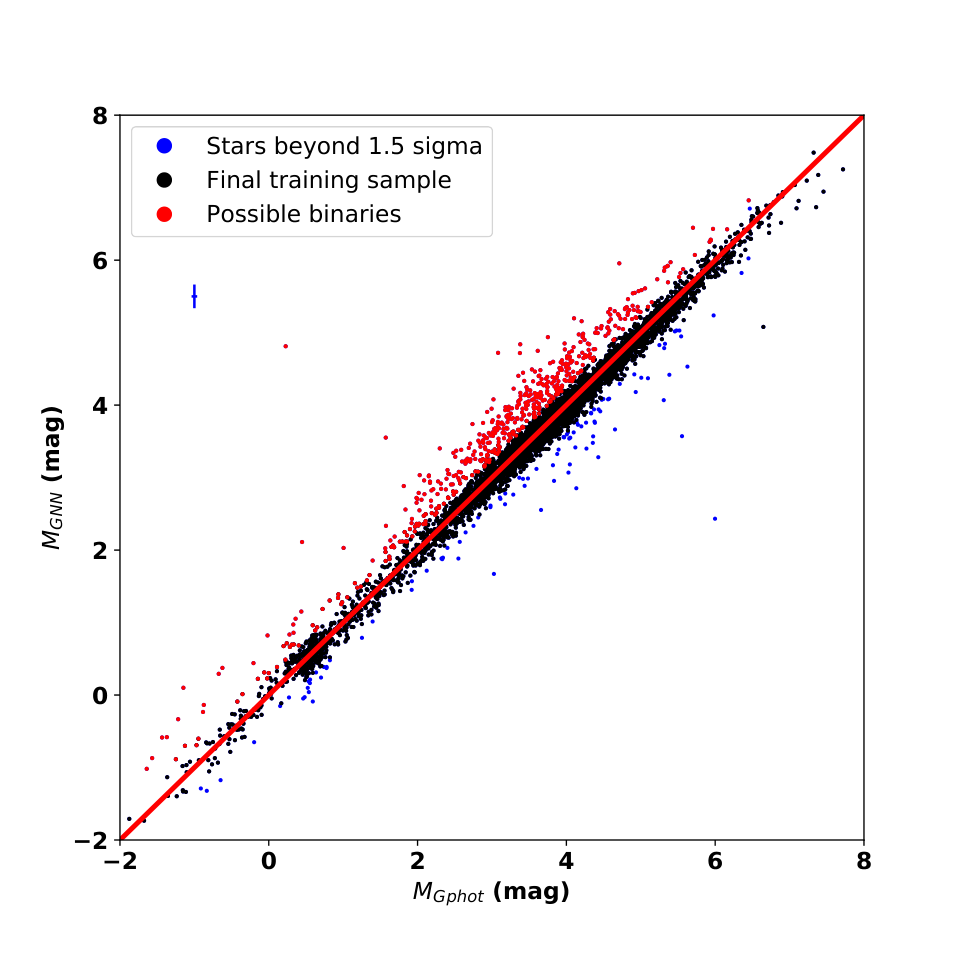
Using the aforementioned neural network models based on the LGMWAS training stars, we estimate the aforementioned absolute magnitudes for training stars. Fig. 4 shows the comparison of photometric absolute magnitudes (estimated based on distance modulus) and absolute magnitudes derived from LAMOST spectra for Gaia EDR3 band of our LGMWAS training stars. There are some stars (red dots) of which the photometric absolute magnitudes are brighter than that derived from LAMOST spectra. These stars are most likely binary stars. In order to obtain a more reliable relation between LAMOST spectra and absolute magnitudes, we exclude these possible binary stars from our LGMWAS training sample. We also exclude stars (blue dots) beyond 1.5 sigma through sigma clipping process except stars with . Then new final LGMWAS training stars (black dots) are adopted to build up the final neural network models.
We adopt the final LGMWAS training sample to obtain the neural network models between the LAMOST spectra and aforementioned absolute magnitudes, and then estimate absolute magnitudes using LAMOST spectra for test stars. We find that the photometric absolute magnitudes (estimated based on distance modulus) and absolute magnitudes derived from LAMOST spectra could match with each other very well. The standard deviations of the residuals are only 0.132, 0.127, 0.136, 0.139, 0.139, 0.134, 0.157, 0.143, 0.148, 0.232, 0.143, 0.153, 0.138 and 0.143 mag for the of Gaia, of 2MASS, of APASS, of SDSS and of WISE bands, respectively. The systematic differences between photometric absolute magnitudes and that derived from LAMOST spectra are very small, almost all of them are smaller than 0.02 mag. One can see Fig. A3 in Appendix for more details of the comparisons.
It is noted that the three training sets have few common sources. The LAMOST-PASTEL and LAMOST-APOGEE have 117 common stars, LAMOST-APOGEE and LGMWAS have 116 common stars and LAMOST-PASTEL and LGMWAS only have one common star. Because of that one parameter has one individual neural network model, which suggest that the stellar parameters are estimated independently, the few common stars do not affect the quality of the estimated stellar parameters.
The catalogs of the three training sets in FITS format will be published in http://www.lamost.org/dr8/v1.0/doc/vac together with our final value-added catalog.

IV Applying neural-network models to LAMOST DR8 low-resolution spectra
After building up neural network models based on aforementioned three training sets, we apply them to all LAMOST DR8 low-resolution spectra and estimate the absolute magnitudes, effective temperatures, surface gravity, metallicity and chemical element abundances. After estimating these stellar parameters, we study the quality of our results.
In this section, we will first estimate the uncertainties of the estimated stellar parameters using neural network method through internal comparison. Secondly, we further check the quality of our estimates through external comparisons for all kinds of stellar parameters. The external comparisons will also help us to check whether our estimations exist systematic errors.
IV.1 The uncertainties of the stellar parameters estimated using neural network method
In this section, we examine the uncertainties of the stellar parameters estimated using neural network method. The uncertainties of these deduced stellar parameters are dependent on the spectral noise (random errors) and method errors. It is noted that the uncertainties are also dependent on stellar parameters as discussed in the following chapters. We do not discuss the dependence on stellar parameters of the uncertainties here.
The random errors of derived stellar parameters are estimated through comparing results derived from duplicate observations of similar spectral SNRs (differed by less than 10%) collected during different nights. Fig. 5 shows the relative stellar parameter estimate residuals (after divided by ) variations with mean spectral SNRs. In order to obtain proper random errors of stellar parameters, we fit the relative residuals with the similar equation of Huang et al. 2020:
| (2) |
where represents the random error. Note that, the relative residuals are divided by 100 when we do this fit for . Besides the random errors, method errors () are also considered when we estimate the uncertainties of stellar parameters. The final errors are given by . The method errors are provided by the relative residuals between our estimated results and the results respectively provided by PASTEL, APOGEE or distance modulus of the responding training sample. The resulting fit coefficients of random errors and method errors for different stellar parameters are presented in Table 2.
| Parameters | a | b | c | |
|---|---|---|---|---|
| 0.210 | 1.229 | 42.827 | 75 | |
| _PASTEL | 0.047 | 1.121 | 7.818 | 0.089 |
| _PASTEL | 0.028 | 1.156 | 5.817 | 0.049 |
| _APOGEE | 0.0097 | 0.993 | 2.332 | 0.033 |
| 0.011 | 1.029 | 2.677 | 0.032 | |
| 0.0075 | 1.084 | 1.557 | 0.018 | |
| 0.010 | 1.029 | 1.913 | 0.043 | |
| 0.022 | 1.095 | 2.634 | 0.070 | |
| _APOGEE | 0.028 | 1.141 | 6.829 | 0.067 |
| G_Gaia | 0.049 | 1.048 | 10.442 | 0.092 |
| Bp_Gaia | 0.051 | 1.055 | 9.980 | 0.075 |
| Rp_Gaia | 0.057 | 1.097 | 12.347 | 0.090 |
| J_2MASS | 0.052 | 1.019 | 10.435 | 0.081 |
| H_2MASS | 0.052 | 1.090 | 12.451 | 0.082 |
| Ks_2MASS | 0.053 | 1.014 | 9.026 | 0.088 |
| B_APASS | 0.053 | 1.062 | 11.734 | 0.096 |
| V_APASS | 0.055 | 1.102 | 12.518 | 0.087 |
| r_APASS | 0.053 | 1.063 | 10.905 | 0.095 |
| g_SDSS | 0.056 | 1.076 | 11.733 | 0.157 |
| r_SDSS | 0.050 | 1.052 | 10.298 | 0.103 |
| i_SDSS | 0.054 | 1.068 | 11.538 | 0.098 |
| W1_WISE | 0.052 | 1.037 | 10.468 | 0.097 |
| W2_WISE | 0.050 | 1.021 | 10.236 | 0.100 |

IV.2 Comparing our effective temperature with that provided by -ESO and APOGEE DR16
The -ESO Public Spectroscopic Survey is designed to obtain high quality and high resolution spectra of some 100 000 Milky Way stars (Gilmore et al. 2012; Smiljanic et al. 2014; Worley et al. 2020). -ESO observed stars using the medium-resolution spectrograph GIRAFFE ( 20 000) and the high-resolution spectrograph UVES (47 000) mounted on the VLT. -ESO DR3 have provided accurate stellar atmospheric parameters and chemical abundances for stars observed by -ESO Survey before July 2014. As discussed in Section 3.2, APOGEE DR16 provides accurate estimates of effective temperatures and chemical element abundances using high resolution spectra. Thus we could test the accuracy of our effective temperature measurements by comparing our results with independent measurements from the -ESO and APOGEE surveys.
Through cross matching LAMOST DR8 and -ESO DR3, we obtain 167 common stars, of which the LAMOST spectral SNR is larger than 20, the typical uncertainties of and [Fe/H] provided by -ESO DR3 for FGK type stars are 55 K and 0.07 dex, respectively. We also obtain 53,295 common stars, with LAMOST spectral SNR larger than 20, APOGEE spectral SNR larger than 70, uncertainties of [Fe/H], and provided by APOGEE DR16 smaller than 0.1 dex, 150 K and 0.15 dex, and of APOGEE higher than 4000 K, through cross matching APOGEE DR16 and LAMOST DR8.
In the Fig. 6, we compare effective temperatures provided by -ESO DR3 and APOGEE DR16 with effective temperatures derived from LAMOST spectra based on neural-network models using LAMOST-PASTEL as training set of the current works. We find that the differences of our measurements with the -ESO DR3 and APOGEE DR16 measurements have sigma of 127.1 K and 111.5 K, respectively. The systematic differences of our measurements with the -ESO DR3 and APOGEE DR16 measurements are respectively 14.7 K and K, which are negligible considering the typical uncertainties of stellar atmospheric parameters provided by -ESO DR3 and APOGEE DR16.

IV.3 Comparisons of our surface gravity with asteroseismic measurements and that of APOGEE DR16
In this section, we examine the quality of surface gravity measurements using the LAMOST-PASTEL (-NN-PASTEL) and the LAMOST-APOGEE (-NN-APOGEE) stellar sample as training sets.
In order to test the quality of estimated surface gravity, we compare our values of surface gravity with asteroseismic measurements and that of APOGEE DR16. APOGEE DR16 provide accurate stellar parameters including accurate surface gravity. The asteroseismic surface gravity () estimates inferred from the data can be accurate to 0.03 dex (Hekker et al. 2013; Huber et al. 2014), which is even much better than that estimated with high-resolution spectroscopy (0.1 dex). Cross matching targets and LAMOST DR8 targets, we find 4 000 common stars with LAMOST spectral SNR and error of asteroseismic surface gravity Err dex.
Fig. 7 shows the comparisons between our two kinds of estimates and asteroseismic and APOGEE for common stars with LAMOST spectral SNR . From this figure, we can find that our estimated using LAMOST-APOGEE as training set could match very well with the asteroseismic and APOGEE . The offset of the difference of our -NN-APOGEE with asteroseismic and APOGEE are negligible. The standard deviations are only 0.095 and 0.109 dex for the difference of our -NN-APOGEE with asteroseismic and APOGEE , respectively. The estimated using LAMOST-PASTEL as training set could match very well with asteroseismic or APOGEE for dwarf stars. However, our -NN-PASTEL for giant stars are over estimated with 0.25 dex. The offset of the difference of our -NN-PASTEL with asteroseismic and APOGEE are and dex. The standard deviations are only 0.18 and 0.214 dex for the difference of our -NN-PASTEL with asteroseismic our and APOGEE , respectively. The -NN-APOGEE are better than the -NN-PASTEL for stars with K, especially for giant stars.

IV.4 The external comparisons of [Fe/H] values
In this section, we examine the quality of [Fe/H] measurements using the LAMOST-PASTEL ([Fe/H]-NN-PASTEL) and LAMOST-APOGEE ([Fe/H]-NN-APOGEE) stellar samples as training sets. We compare our [Fe/H] values with that of -ESO Survey and APOGEE DR16 to verify whether our [Fe/H] have systematic errors. In addition, the [Fe/H] dispersions of member stars in open clusters are also studied to check the uncertainties of metallicity.
IV.4.1 Comparisons with -ESO Survey
As discussed in section 4.2, the -ESO DR3 have derived accurate stellar atmospheric parameters and chemical element abundances using the medium and high-resolution spectra. We test the accuracy of the two kinds of [Fe/H] measurements through comparing with that provided by -ESO DR3. Fig. 8 shows the comparisons between our two kinds of [Fe/H] measurements with [Fe/H] provided by -ESO DR3. We find that the differences of [Fe/H] values provided by -ESO DR3 with [Fe/H]-NN-PASTEL and [Fe/H]-NN-APOGEE have standard deviation of 0.143 dex and 0.105 dex, respectively. The systematic differences of [Fe/H] of -ESO DR3 with [Fe/H]-NN-PASTEL and [Fe/H]-NN-APOGEE are respectively dex and dex. The comparison suggests that our [Fe/H] measurements using the LAMOST-PASTEL and LAMOST-APOGEE stellar samples as training sets could match well with the [Fe/H] values of -ESO.
IV.4.2 Comparison with APOGEE DR16
We also compare our two kinds of [Fe/H] measurements with that provided by APOGEE DR16 in order to test the quality of our [Fe/H] values. Fig. 9 shows the comparisons. We find that the differences of [Fe/H] values provided by APOGEE with [Fe/H]-NN-PASTEL and [Fe/H]-NN-APOGEE have standard deviations of 0.125 dex and 0.052 dex, respectively. The systematic differences of [Fe/H] of APOGEE with [Fe/H]-NN-PASTEL and [Fe/H]-NN-APOGEE are respectively dex and dex. The comparison suggests that our [Fe/H] measurements using the LAMOST-PASTEL and LAMOST-APOGEE stellar samples as training sets could match well with the [Fe/H] values of APOGEE DR16.
IV.4.3 The [Fe/H] values of the candidates of open cluster members
Stars in open cluster (OC) are believed to form almost simultaneously from a single gas cloud, thus they have almost the same metallicity. Thus, OC is a good test bed to check the uncertainty of metallicity determinations. 8,811 cluster member stars observed by LAMOST have been provided by Zhong et al. 2020a and Zhong et al. 2020b, who cross-match the cluster member stars of OCs provided by Cantat-Gaudin et al. 2018 with LAMOST DR5. Here, we simply test the uncertainties of our metallicity estimates using these cluster members. We select cluster members in four OCs of , , , (there are enough number of cluster members targeted by LAMOST in these four OCs) with spectral SNR and K to do the test.
Fig. 10 shows the [Fe/H] (using LAMOST-PASTEL common stars as training set) variations with for cluster members in the aforementioned four OCs. From this figure, we can find that the standard deviations of the metallicity distributions of cluster members in these four OCs are almost similar with (or slightly larger than) the uncertainties of our metallicity determinations. The metallicity have no trend with when 4 500–4 750 K. The metallicity of stars with 4 500–4 750 K are underestimated, most of these stars are dwarf stars (cool dwarf stars). As shown in Fig. 1 and Fig. 11, the LAMOST-PASTEL training sample only has few cool dwarf stars. Stars with significantly underestimated [Fe/H] values are almost located outside the LAMOST-PASTEL training parameter grid as shown in Fig. 11.
Fig. 12 shows the [Fe/H] (using LAMOST-APOGEE common stars as training set) variations with of cluster members in the aforementioned four OCs. We can find that the standard deviations of the metallicity distributions of these cluster members are almost similar with the uncertainty of our metallicity determinations. The metallicity have no trend with when 4 500–4 750 K for cluster members in these four OCs. The metallicity of stars with 4 500–4 750 K are slightly underestimated for stars in these four OCs. Similar with the results of [Fe/H] values estimated using LAMOST-PASTEL common stars as training set, the underestimations of metallicity may be the consequence of the lack of cool dwarf training stars. The metallicity underestimates of cool dwarfs here are much better than that estimated using LAMOST-PASTEL common stars as training set, through comparing Fig. 10 and Fig. 12.


IV.5 The external comparisons of [M/H], [/M], [C/Fe] and [N/Fe] values
In this section, we examine the quality of [M/H], [/M], [C/Fe] and [N/Fe] measurements using LAMOST-APOGEE stellar sample as training set. We first compare our chemical abundance values with that of APOGEE DR16 to study the uncertainties and systematic errors of them. The chemical abundance dispersions of member stars in OCs are also studied to check the uncertainties of them.
IV.5.1 Comparisons with APOGEE DR16
We compare our estimates of [M/H], [/M], [C/Fe] and [N/Fe] with that of APOGEE DR16 in order to study the quality of our estimates.
Fig. 13 shows the comparison results. Our estimates of [M/H], [/Fe], [C/Fe] and [N/Fe] could match well with those provided by APOGEE DR16. We find that the differences of [M/H], [/Fe], [C/Fe] and [N/Fe] between our estimates and those of APOGEE DR16 have standard deviations of 0.05 dex, 0.028 dex, 0.055 dex and 0.085 dex, respectively. The systematic differences of [M/H], [/Fe], [C/Fe] and [N/Fe] between the two estimates are respectively dex, dex, dex and dex. The offsets are so small that could be ignored. These results are suitable for LAMOST spectra with spectral SNR , the dispersion of the difference will be much smaller for the results of stars with higher quality LAMOST spectra.

IV.5.2 The chemical abundances of the candidates of open cluster members
As discussed in Section 4.4.3, OC is a good test bed to check the uncertainties of chemical abundance determinations. Here, we briefly study the uncertainties of chemical abundances estimated by our neural network models using LAMOST-APOGEE common stars as training set of LAMOST cluster members identified by Zhong et al. 2020a and Zhong et al. 2020b.
Fig. 14, Fig. 15, Fig. 16 and Fig. 17 show respectively, the [M/H], [/M], [C/Fe] and [N/Fe] variations with of stellar members in the aforementioned four OCs. The results of [M/H] are similar with our [Fe/H] using LAMOST-APOGEE as training set. The variations of [/M], [C/Fe] and [N/Fe] with are very small, except for the underestimated [N/Fe] of stars with K. The underestimations of [N/Fe] of stars with K may be the consequence of lack of cool dwarf stars in the training set as discussed in section 4.4.3. Fig. 18 shows the distributions of stars with significant underestimated [N/Fe] in the – plane. We can find that these stars are almost located outside the training parameter grid or at the edge of the training parameter grid. From Fig. 14, Fig. 15, Fig. 16 and Fig. 17, one can see that the standard deviations of [M/H], [/Fe], [C/Fe] and [N/Fe] of stellar members in these four OCs are very small. Thus our estimates of [M/H], [/Fe], [C/Fe] and [N/Fe] are very good.
During red giant stage, the dredge-up process change the surface chemical abundance because of the convective mixing, which will finally decrease the surface abundance ratio of [C/N] (Casali et al. 2019; Bertelli Motta et al. 2017, e.g.,). As shown in Fig. 19, we find a clear decrease of [C/N] from of dwarf stars to of giant stars in the open cluster of (M67), which is consistent with the results of Casali et al. 2019 and Bertelli Motta et al. 2017. Our estimated [C/Fe] and [N/Fe] could well reproduce the variations of [C/N] of red giant stars in open clusters. [C/N] ratios are tightly correlated with the stellar masses for red giants and thus can be further used to derive their ages using the relation of [C/N] and stellar masses (Martig et al. 2016; Ness et al. 2016, e.g.,). One can use the estimated [C/Fe] and [N/Fe] values here of red giant stars to derive their stellar ages.


IV.6 The external comparisons of absolute magnitudes
We test the quality of our estimates of absolute magnitudes through comparing with photometric absolute magnitudes. Through cross-matching the LAMOST DR8 and Gaia EDR3, 2MASS, APASS, SDSS and WISE, we obtain 66,498 common stars. They have accurate estimations of distances, apparent magnitudes, interstellar extinctions and high quality LAMOST spectra (with spectral SNR ). For these stars we could estimate accurate photometric absolute magnitudes based on the distance modulus. Then we compare our estimated absolute magnitudes with the photometric absolute magnitudes in order to evaluate the quality of our estimates of absolute magnitudes.
Fig. 20 shows the comparison results. The two kinds of absolute magnitudes could match with each other very well. We find that the differences of the , between the two kinds estimates have of 0.251, 0.243, 0.245, 0.247, 0.241, 0.237, 0.273, 0.26, 0.257, 0.326, 0.266, 0.262, 0.238 and 0.245 mag, respectively. These are equivalent to the distance error of 15%. The absolute value of systematic differences of absolute magnitudes of these bands are almost smaller than 0.1 mag.

In conclusion, the stellar parameters estimated using neural network method have small uncertainties through comparing results derived from duplicate observations of similar spectral SNRs (differed by less than 10%) collected during different nights. For stars with spectral SNRs larger than 50, precisions of , (estimated using LAMOST-APOGEE common stars as training set), [Fe/H] (estimated using LAMOST-APOGEE common stars as training set), [M/H], [C/Fe], [N/Fe] and [/M] are 85 K, 0.098 dex, 0.05 dex, 0.05 dex, 0.052 dex, 0.082 dex and 0.027 dex, respectively. The errors of 14 band’s absolute magnitudes are only 0.16–0.22 mag for stars with spectral SNRs larger than 50. As discussed in Section 3, the , [Fe/H] have two values for each star estimated using different stellar sample as training set (LAMOST-PASTEL common stars, LAMOST-APOGEE common stars). Precisions of and [Fe/H] estimated using LAMOST-PASTEL common stars as training set are 0.135 dex and 0.08 dex for stars with spectral SNRs larger than 50. Our stellar parameters could match well with other external parameter catalogs, including Gaia-ESO, APOGEE (for , , [Fe/H], [M/H], [C/Fe], [N/Fe] and [/M] comparisons), catalog of asteroseismic measurements (for comparisons) and catalog of photometric absolute magnitudes (for absolute magnitude comparisons). For metallicity and chemical abundance ratios, we also studied the dispersions of stars in open clusters. The dispersions are very small.
V The [Fe/H] values of very metal poor stars
Very metal poor (VMP) stars ([Fe/H] ) provide the fossil record of the early chemical history of the Galaxy and early generations of stars. In this section, we will present the improved estimates for VMP candidates using the neural network method.
Firstly, we select 65,465 stars with [Fe/H] and K as VMP candidates and re-estimate their [Fe/H] values. In this process, we only use metal poor stars ([Fe/H] ) in the pre-mentioned LAMOST–PASTEL training sample as training stars. Because the spectral features of VMPs are dominated in the blue range of LAMOST spectra, we only use 3900–4400 Å to determine the [Fe/H] values for metal poor stars. Our final neural network model contain two layers. The neurons of the first and second layer of neural network model are respectively 256 and 64. Using the neural network model based on the metal poor stars as training set, we estimate the [Fe/H] values for training stars using LAMOST spectra and compare with that provided by PASTEL. The standard deviations of the residuals and systematic difference are only 0.176 and -0.01 dex, respectively. The improved [Fe/H] values ([Fe/H]-NN-VMP) here could match well with that provided by PASTEL at [Fe/H] dex. One can see Fig. A4 in Appendix for more details about the comparisons between the improved [Fe/H] values and that provided by PASTEL. After building up neural network model, we apply them to all LAMOST low-resolution spectra of these VMP candidates and estimate the improved [Fe/H] values.
Li et al. 2018 provide a catalog of 10,008 VMPs from LAMOST DR3, which is the largest number of VMP candidates. The [Fe/H] values of these VMP stars are derived from LAMOST low resolution spectra. 70 of stars in these stars have high-resolution spectroscopic analyses reported in the literature (Fulbright 2000; Carretta et al. 2002; Cohen et al. 2004; Cohen et al. 2006; Cohen et al. 2013; Honda et al. 2004; Aoki et al. 2005; Arnone et al. 2005; Barklem et al. 2005; Lai et al. 2007; Lai et al. 2008; Andrievsky et al. 2009; Andrievsky et al. 2010; Rich & Boesgaard 2009; Meléndez et al. 2010; Caffau et al. 2011; Hollek et al. 2011; Suda et al. 2011; Allen et al. 2012; Bonifacio et al. 2012; Yong et al. 2013; Placco et al. 2014; Roederer et al. 2014; Placco et al. 2014; Li et al. 2015a; Li et al. 2015b; Li et al. 2018; Jacobson et al. 2015; Matsuno et al. 2017). Through comparing our un-improvded ([Fe/H]-NN-PASTEL) and improved [Fe/H] values with previous [Fe/H] estimates for VMP candidates, the accuracy of [Fe/H] values of our VMP candidates could be tested.
Fig. 21 shows the comparisons between our two kinds of [Fe/H] values ([Fe/H]-NN-PASTEL and [Fe/H]-NN-VMP) and [Fe/H] values (derived from LAMOST low resolution spectra: [Fe/H]-Li-L) provided by Li et al. 2018. The systematic difference between [Fe/H]-NN-PASTEL and [Fe/H]-Li-L is 0.014 dex, the sigma of the corresponding difference is 0.299 dex. It is noted that the systematic differences between the [Fe/H]-NN-PASTEL and [Fe/H]-Li-L vary with metallicity, [Fe/H]-NN-PASTEL are underestimated and overestimated for stars with high metallicity ([Fe/H] dex) and low metallicity ( [Fe/H] dex), respectively. However, the systematic differences are almost smaller than 0.4 dex for stars with [Fe/H] . For the [Fe/H]-NN-VMP, the systematic difference and the sigma for the comparison with [Fe/H]-Li-L are respectively only -0.044 dex and 0.219 dex. The [Fe/H]-NN-VMP are overestimated for stars with metallicity of [Fe/H] dex. The overestimations of the [Fe/H]-NN-VMP is smaller than that of [Fe/H]-NN-PASTEL.
Fig. 22 shows the comparison between our two kinds of [Fe/H] values and [Fe/H] values analysed based on high-resolution spectra. We find that the difference with the [Fe/H] values of high-resolution of [Fe/H]-NN-PASTEL and [Fe/H]-NN-VMP have sigma of 0.452 dex and 0.35 dex, respectively. The average measurement offset of [Fe/H]-NN-PASTEL and [Fe/H]-NN-VMP are respectively -0.222 dex and -0.086 dex. The [Fe/H]-NN-VMP could match well with that derived from high resolution spectra for stars with [Fe/H] dex.
Through comparing with [Fe/H]-Li-L and [Fe/H] values of high-resolution, we suggest that the [Fe/H]-NN-VMP are much better than the [Fe/H]-NN-PASTEL for stars with [Fe/H] dex. Based on the [Fe/H]-NN-VMP values, we select 26,868 unique stars with SNR larger than 20 as VMP candidates ([Fe/H] dex). Among of them, 3,952 unique stars have [Fe/H] dex. Our catalog will provide the largest number of VMP candidates up to now.
VI Distance
Now many distances of stars in the Milky Way could be derived using parallax provided by Gaia EDR3. The errors of parallaxes provided by Gaia EDR3 depend on the distance of stars. For distances larger than 2.0 kpc, the systematic errors of parallax-based distance estimates become significant (Lindegren et al. 2018; Huang et al. 2021; Lindegren et al. 2021a; Lindegren et al. 2021b; Ren et al. 2021; Xiang et al. 2021a). For stars with distances larger than 2.0 kpc, spectro-photometric distance estimation is a better choice. The accuracy of spectro-photometric distance does not depend on itself.
We provide spectro-photometric distance based on absolute magnitudes directly derived from the LAMOST spectra. Distance of individual stars observed by LAMOST are estimated with distance modulus method using the apparent magnitudes, interstellar extinctions and our absolute magnitudes. Here, we adopt to calculate distance, as it suffers from less severe extinction than other bands. After estimating distance, we estimate the distance errors based on the principle of uncertainty propagation. In doing so, errors of absolute magnitudes, extinction and apparent magnitudes are considered. The spectro-photometric distances are accurate to 8.5% for stars with spectral SNRs larger than 50.
Fig. 23 shows the variations of systematic difference of our spectro-photometric distance and geometrical distance provided by Gaia EDR3 with our spectro-photometric distance. We can find that systematic difference is 0 at kpc, which suggest that geometrical distance could match well with spectro-photometric distance for stars with kpc. However, for stars with distance larger than 2.0 kpc, the systematic difference become larger with distance increasing. Up to 8 kpc, the geometrical distances are underestimated about 25 per cent, which is similar with that of Xiang et al. 2021a.

VII The value-added catalog
After estimating aforementioned stellar parameters, we build up a value-added catalog for LAMOST DR8 low-resolution stellar spectra. The value-added catalog contains the stellar atmospheric parameters (, and [Fe/H]/[M/H]), chemical abundance ratios ([/M], [C/Fe] and [N/Fe]), 14 band’s absolute magnitudes ( of Gaia EDR3 bands, of 2MASS bands, of WISE bands, of APASS bands and of SDSS bands) and spectro-photometric distances of 7,109,030 spectra of 5,166,619 unique stars. The value-added catalog contains stellar parameters for all LAMOST spectra with SNRs larger than 10. Because of bad LAMOST spectra, the effective stellar parameter range of training sets as discussed in section 3 and systematic errors of stellar parameters for some stars as discussed in section 4, some stellar parameter estimates are not so accurate. One need make some selection criteria of stellar parameters according to their science goals. Extinctions from Huang et al. (2021) are also given. The catalog also provide the radial velocities derived by LASP. A detailed description of the catalog content is presented in Table 3. The catalog will be released in the website of http://www.lamost.org/dr8/v1.0/doc/vac.
We estimate 3D positions in the right-handed Cartesian system (, , with toward the direction opposite to the Sun, in the direction of Galactic rotation, and toward the north Galactic pole). Fig. 24 shows the spatial stellar number density distributions of our stellar sample in the – and – planes. This figure suggests that our sample covers a large volume of the Milky Way. One can use it to probe the structural, kinematic and chemical properties of the Galactic disc combining the proper motions provided by Gaia EDR3. Fig. 25 shows the stellar number density distributions of stars in the –, – and ()– planes. Fig. 26 shows the stellar number density distributions of our stellar sample in the [Fe/H]-[/M] plane for dwarfs and giants. The two figures suggest that the stellar parameters of our sample span wide ranges, contain numerous dwarf stars, main-sequence turn-off stars, giant stars, metal-poor and metal-rich stars. One could build up different stellar sample for different scientific goals using this value-added catalog.
| Field | Description | Unit |
|---|---|---|
| gaiaid | Cross-matched Gaia EDR3 source ID | – |
| obsid | Unique number ID of this spectrum | – |
| ra_obs | Right ascension from the LAMOST (J2000) | degree |
| dec_obs | Decl. from the LAMOST (J2000) | degree |
| gl | Galactic longitude derived from ICRS coordinates | degree |
| gb | Galactic latitude derived from ICRS coordinates | degree |
| snrg | The LAMOST spectral SNRs in band | 1 |
| rv | Radial velocity | |
| Err_rv | Error of radial velocity | |
| _PASTEL | Effective temperature estimated with neural network using LAMOST-PASTEL sample as training set | K |
| Err__PASTEL | Errors of _PASTEL | K |
| _PASTEL | Surface gravity estimated with neural network using LAMOST-PASTEL sample as training set | dex |
| Err__PASTEL | Errors of _PASTEL | dex |
| _APOGEE | Surface gravity estimated with neural network using LAMOST-APOGEE sample as training set | dex |
| Err__APOGEE | Errors of _APOGEE | dex |
| feh_PASTEL | The value of [Fe/H] with neural network using LAMOST-PASTEL sample as training set | dex |
| Err_feh_PASTEL | Errors of feh_PASTEL | dex |
| feh_APOGEE | The value of [Fe/H] with neural network using LAMOST-APOGEE sample as training set | dex |
| Err_feh_APOGEE | Errors of feh_APOGEE | dex |
| feh_VMP | The improved [Fe/H] values of VMP candidates | dex |
| Err_feh_VMP | Errors of feh_VMP | dex |
| MH_APOGEE | The value of [M/H] with neural network using LAMOST-APOGEE sample as training set | dex |
| Err_MH_APOGEE | Errors of the [M/H] | dex |
| AFE_APOGEE | The value of [/M] with neural network using LAMOST-APOGEE sample as training set | dex |
| Err_AFE_APOGEE | Errors of the [/M] | dex |
| CFE_APOGEE | The value of [C/Fe] with neural network using LAMOST-APOGEE sample as training set | dex |
| Err_CFE_APOGEE | Errors of the [C/Fe] | dex |
| NFE_APOGEE | The value of [N/Fe] with neural network using LAMOST-APOGEE sample as training set | dex |
| Err_NFE_APOGEE | Errors of the [N/Fe] | dex |
| dist_phot | Distances estimated based on distance modulus | kpc |
| Err_dist_phot | Errors of distances | kpc |
| a_gg | Absolute magnitude of EDR3 band | mag |
| Err_a_gg | Error of absolute magnitude of EDR3 band | mag |
| a_bp | Absolute magnitude of EDR3 band | mag |
| Err_a_bp | Error of absolute magnitude of EDR3 band | mag |
| a_rp | Absolute magnitude of EDR3 band | mag |
| Err_a_rp | Error of absolute magnitude of EDR3 band | mag |
| a_j | Absolute magnitude of 2MASS band | mag |
| Err_a_j | Error of absolute magnitude of 2MASS band | mag |
| a_h | Absolute magnitude of 2MASS band | mag |
| Err_a_h | Error of absolute magnitude of 2MASS band | mag |
| a_ks | Absolute magnitude of 2MASS band | mag |
| Err_a_ks | Error of absolute magnitude of 2MASS band | mag |
| a_w1 | Absolute magnitude of WISE band | mag |
| Err_a_w1 | Error of absolute magnitude of WISE band | mag |
| a_w2 | Absolute magnitude of WISE band | mag |
| Field | Description | Unit |
| Err_a_w2 | Error of absolute magnitude of WISE band | mag |
| a_bap | Absolute magnitude of APASS band | mag |
| Err_a_bap | Error of absolute magnitude of APASS band | mag |
| a_rap | Absolute magnitude of APASS band | mag |
| Err_a_rap | Error of absolute magnitude of APASS band | mag |
| a_vap | Absolute magnitude of APASS band | mag |
| Err_a_vap | Error of absolute magnitude of APASS band | mag |
| a_gsd | Absolute magnitude of SDSS band | mag |
| Err_a_gsd | Error of absolute magnitude of SDSS band | mag |
| a_rsd | Absolute magnitude of SDSS band | mag |
| Err_a_rsd | Error of absolute magnitude of SDSS band | mag |
| a_isd | Absolute magnitude of SDSS band | mag |
| Err_a_isd | Error of absolute magnitude of SDSS band | mag |
| X/Y/Z | 3D positions in the right-handed Cartesian system | kpc |
| Err_X/Y/Z | Errors of 3D positions in the right-handed Cartesian system | kpc |
| EBV | interstellar extinctions estimated using “star-pair” method | – |
| uqflag | Uniqueness flag. 1 denoting the spectrum of the highest snr_g of one star | – |
| flag_parameter | The quality flaga on every parameter | unit |
a The flag takes the values of 0 and 1. Flag = 0 means that the parameter estimates
are within the training grid, the estimates are reliable. Flag =1 means that the parameter estimates
are beyond the training grid, the estimates are unreliable.
VIII Summary
In the current work, we build up a value-added catalog for over 7.10 million LAMOST DR8 low-resolution stellar spectra with spectral SNR 10 of million unique stars. We obtain the stellar atmospheric parameters (, and [Fe/H]/[M/H]), chemical element abundances ([/M], [C/Fe] and [N/Fe]), 14 bands’ absolute magnitudes ( of Gaia EDR3 bands, of 2MASS bands, of WISE bands, of APASS bands and of SDSS bands) and spectro-photometric distances using LAMOST spectra.
Based on neural network method adopting LAMOST-PASTEL sample as training set, we have estimated the , and [Fe/H]. The accuracy of , and [Fe/H] are respectively 84.87 K, 0.135 dex and 0.08 dex for stars with LAMOST spectral SNR . Based on neural network method adopting LAMOST-APOGEE sample as training set, we have derived [Fe/H], [M/H], [/M], [C/Fe], [N/Fe] and . The accuracy of [Fe/H], [M/H], [/M], [C/Fe], [N/Fe] and are respectively 0.05 dex, 0.05 dex, 0.027 dex, 0.052 dex, 0.082 dex and 0.098 dex for stars with LAMOST spectral SNR . Based on neural network method adopting LGMWAS sample as training set, the 14 bands’ absolute magnitudes have been derived. The uncertainties of of Gaia EDR3 bands, of 2MASS bands, of APASS bands, of SDSS bands and of WISE bands are respectively 0.176, 0.163, 0.177, 0.186, 0.173, 0.177, 0.187, 0.174, 0.179, 0.221, 0.180, 0.184, 0.185 and 0.190 mag for stars with LAMOST spectral SNR . Using our accurate absolute magnitude of , interstellar extinction and apparent magnitudes, we have derived the spectro-photometric distances based on the method of distance modulus. The accuracy of spectro-photometric distance is 8.5% for stars with LAMOST spectral SNR .
Benefiting from the good estimation of [Fe/H] values for metal poor stars, our catalog provide a largest number of VMP candidates (26,868 unique stars with [Fe/H] dex) up to know. Among of them, 3,952 unique stars have [Fe/H] dex. These VMP candidates will play important roles in the study of searching for the first stellar populations and the study of the Milky Way halo. For stars with kpc, our spectro-photometric distance are better than geometrical distance.
The final sample contain a large number of stars, cover a large and contiguous sky coverage and has simple yet non-trivial target selection function. One can use it to probe the structural, kinematic and chemical properties of the MW combining the proper motions provided by Gaia EDR3.
References
- Allen et al. (2012) Allen, D. M., Ryan, S. G., Rossi, S., Beers, T. C., & Tsangarides, S. A. 2012, A&A, 548, A34, doi: 10.1051/0004-6361/201015615
- Andrievsky et al. (2010) Andrievsky, S. M., Spite, M., Korotin, S. A., et al. 2010, A&A, 509, A88, doi: 10.1051/0004-6361/200913223
- Andrievsky et al. (2009) —. 2009, A&A, 494, 1083, doi: 10.1051/0004-6361:200810894
- Aoki et al. (2005) Aoki, W., Honda, S., Beers, T. C., et al. 2005, ApJ, 632, 611, doi: 10.1086/432862
- Arnone et al. (2005) Arnone, E., Ryan, S. G., Argast, D., Norris, J. E., & Beers, T. C. 2005, A&A, 430, 507, doi: 10.1051/0004-6361:20041034
- Bailer-Jones et al. (2021) Bailer-Jones, C. A. L., Rybizki, J., Fouesneau, M., Demleitner, M., & Andrae, R. 2021, VizieR Online Data Catalog, I/352
- Barklem et al. (2005) Barklem, P. S., Christlieb, N., Beers, T. C., et al. 2005, A&A, 439, 129, doi: 10.1051/0004-6361:20052967
- Bertelli Motta et al. (2017) Bertelli Motta, C., Salaris, M., Pasquali, A., & Grebel, E. K. 2017, MNRAS, 466, 2161, doi: 10.1093/mnras/stw3252
- Boeche et al. (2018) Boeche, C., Smith, M. C., Grebel, E. K., et al. 2018, AJ, 155, 181, doi: 10.3847/1538-3881/aab5af
- Bonifacio et al. (2012) Bonifacio, P., Sbordone, L., Caffau, E., et al. 2012, A&A, 542, A87, doi: 10.1051/0004-6361/201219004
- Bowen & Vaughan (1973) Bowen, I. S., & Vaughan, A. H., J. 1973, Appl. Opt., 12, 1430, doi: 10.1364/AO.12.001430
- Caffau et al. (2011) Caffau, E., Bonifacio, P., François, P., et al. 2011, Nature, 477, 67, doi: 10.1038/nature10377
- Cantat-Gaudin et al. (2018) Cantat-Gaudin, T., Jordi, C., Vallenari, A., et al. 2018, A&A, 618, A93, doi: 10.1051/0004-6361/201833476
- Carretta et al. (2002) Carretta, E., Gratton, R., Cohen, J. G., Beers, T. C., & Christlieb, N. 2002, AJ, 124, 481, doi: 10.1086/340955
- Casali et al. (2019) Casali, G., Magrini, L., Tognelli, E., et al. 2019, A&A, 629, A62, doi: 10.1051/0004-6361/201935282
- Chen et al. (2016) Chen, B., Liu, X., Xiang, M., et al. 2016, AJ, 152, 45, doi: 10.3847/0004-6256/152/2/45
- Cohen et al. (2013) Cohen, J. G., Christlieb, N., Thompson, I., et al. 2013, ApJ, 778, 56, doi: 10.1088/0004-637X/778/1/56
- Cohen et al. (2004) Cohen, J. G., Christlieb, N., McWilliam, A., et al. 2004, ApJ, 612, 1107, doi: 10.1086/422576
- Cohen et al. (2006) Cohen, J. G., McWilliam, A., Shectman, S., et al. 2006, AJ, 132, 137, doi: 10.1086/504597
- Conroy et al. (2019) Conroy, C., Bonaca, A., Cargile, P., et al. 2019, ApJ, 883, 107, doi: 10.3847/1538-4357/ab38b8
- Cropper et al. (2018) Cropper, M., Katz, D., Sartoretti, P., et al. 2018, A&A, 616, A5, doi: 10.1051/0004-6361/201832763
- Dalton et al. (2014) Dalton, G., Trager, S., Abrams, D. C., et al. 2014, in Society of Photo-Optical Instrumentation Engineers (SPIE) Conference Series, Vol. 9147, Ground-based and Airborne Instrumentation for Astronomy V, ed. S. K. Ramsay, I. S. McLean, & H. Takami, 91470L, doi: 10.1117/12.2055132
- de Jong et al. (2019) de Jong, R. S., Agertz, O., Berbel, A. A., et al. 2019, The Messenger, 175, 3, doi: 10.18727/0722-6691/5117
- De Silva et al. (2015) De Silva, G. M., Freeman, K. C., Bland-Hawthorn, J., et al. 2015, MNRAS, 449, 2604, doi: 10.1093/mnras/stv327
- Deng et al. (2012) Deng, L.-C., Newberg, H. J., Liu, C., et al. 2012, Research in Astronomy and Astrophysics, 12, 735, doi: 10.1088/1674-4527/12/7/003
- Feltzing et al. (2018) Feltzing, S., Bensby, T., Bergemann, M., et al. 2018, in Rediscovering Our Galaxy, ed. C. Chiappini, I. Minchev, E. Starkenburg, & M. Valentini, Vol. 334, 225–232, doi: 10.1017/S1743921317008730
- Fulbright (2000) Fulbright, J. P. 2000, AJ, 120, 1841, doi: 10.1086/301548
- Gaia Collaboration et al. (2020) Gaia Collaboration, Brown, A. G. A., Vallenari, A., et al. 2020, arXiv e-prints, arXiv:2012.01533. https://arxiv.org/abs/2012.01533
- Gaia Collaboration et al. (2016) —. 2016, A&A, 595, A2, doi: 10.1051/0004-6361/201629512
- Gaia Collaboration et al. (2018) —. 2018, A&A, 616, A1, doi: 10.1051/0004-6361/201833051
- Gandhi & Ness (2019) Gandhi, S. S., & Ness, M. K. 2019, ApJ, 880, 134, doi: 10.3847/1538-4357/ab2981
- Gao et al. (2015) Gao, H., Zhang, H.-W., Xiang, M.-S., et al. 2015, Research in Astronomy and Astrophysics, 15, 2204, doi: 10.1088/1674-4527/15/12/008
- García Pérez et al. (2016) García Pérez, A. E., Allende Prieto, C., Holtzman, J. A., et al. 2016, AJ, 151, 144, doi: 10.3847/0004-6256/151/6/144
- Gilmore et al. (2012) Gilmore, G., Randich, S., Asplund, M., et al. 2012, The Messenger, 147, 25
- Gunn et al. (2006) Gunn, J. E., Siegmund, W. A., Mannery, E. J., et al. 2006, AJ, 131, 2332, doi: 10.1086/500975
- Hekker et al. (2013) Hekker, S., Elsworth, Y., Mosser, B., et al. 2013, A&A, 556, A59, doi: 10.1051/0004-6361/201321630
- Ho et al. (2017) Ho, A. Y. Q., Ness, M. K., Hogg, D. W., et al. 2017, ApJ, 836, 5, doi: 10.3847/1538-4357/836/1/5
- Hollek et al. (2011) Hollek, J. K., Frebel, A., Roederer, I. U., et al. 2011, ApJ, 742, 54, doi: 10.1088/0004-637X/742/1/54
- Honda et al. (2004) Honda, S., Aoki, W., Kajino, T., et al. 2004, ApJ, 607, 474, doi: 10.1086/383406
- Huang et al. (2019) Huang, Y., Chen, B. Q., Zhang, H. W., et al. 2019, ApJ, 877, 13, doi: 10.3847/1538-4357/ab158a
- Huang et al. (2018) Huang, Y., Liu, X. W., Chen, B. Q., et al. 2018, AJ, 156, 90, doi: 10.3847/1538-3881/aacda5
- Huang et al. (2015) Huang, Y., Liu, X. W., Yuan, H. B., et al. 2015, MNRAS, 449, 162, doi: 10.1093/mnras/stv204
- Huang et al. (2021) Huang, Y., Yuan, H., Beers, T. C., & Zhang, H. 2021, ApJ, 910, L5, doi: 10.3847/2041-8213/abe69a
- Huang et al. (2016) Huang, Y., Liu, X. W., Yuan, H. B., et al. 2016, MNRAS, 463, 2623, doi: 10.1093/mnras/stw2096
- Huang et al. (2020) Huang, Y., Schönrich, R., Zhang, H., et al. 2020, ApJS, 249, 29, doi: 10.3847/1538-4365/ab994f
- Huber et al. (2014) Huber, D., Silva Aguirre, V., Matthews, J. M., et al. 2014, ApJS, 211, 2, doi: 10.1088/0067-0049/211/1/2
- Jacobson et al. (2015) Jacobson, H. R., Keller, S., Frebel, A., et al. 2015, ApJ, 807, 171, doi: 10.1088/0004-637X/807/2/171
- Jönsson et al. (2020) Jönsson, H., Holtzman, J. A., Allende Prieto, C., et al. 2020, AJ, 160, 120, doi: 10.3847/1538-3881/aba592
- Kamdar et al. (2019) Kamdar, H., Conroy, C., Ting, Y.-S., et al. 2019, ApJ, 884, L42, doi: 10.3847/2041-8213/ab4997
- Kollmeier et al. (2017) Kollmeier, J. A., Zasowski, G., Rix, H.-W., et al. 2017, arXiv e-prints, arXiv:1711.03234. https://arxiv.org/abs/1711.03234
- Lai et al. (2008) Lai, D. K., Bolte, M., Johnson, J. A., et al. 2008, ApJ, 681, 1524, doi: 10.1086/588811
- Lai et al. (2007) Lai, D. K., Johnson, J. A., Bolte, M., & Lucatello, S. 2007, ApJ, 667, 1185, doi: 10.1086/520949
- Lee et al. (2015) Lee, Y. S., Beers, T. C., Carlin, J. L., et al. 2015, AJ, 150, 187, doi: 10.1088/0004-6256/150/6/187
- Li et al. (2015a) Li, H., Aoki, W., Zhao, G., et al. 2015a, PASJ, 67, 84, doi: 10.1093/pasj/psv053
- Li et al. (2018) Li, H., Tan, K., & Zhao, G. 2018, ApJS, 238, 16, doi: 10.3847/1538-4365/aada4a
- Li et al. (2015b) Li, H.-N., Zhao, G., Christlieb, N., et al. 2015b, ApJ, 798, 110, doi: 10.1088/0004-637X/798/2/110
- Li et al. (2016) Li, J., Han, C., Xiang, M.-S., et al. 2016, Research in Astronomy and Astrophysics, 16, 110, doi: 10.1088/1674-4527/16/7/110
- Li et al. (2019) Li, J., FELLOW, L., Liu, C., et al. 2019, ApJ, 874, 138, doi: 10.3847/1538-4357/ab09ef
- Lindegren et al. (2018) Lindegren, L., Hernández, J., Bombrun, A., et al. 2018, A&A, 616, A2, doi: 10.1051/0004-6361/201832727
- Lindegren et al. (2021a) Lindegren, L., Klioner, S. A., Hernández, J., et al. 2021a, A&A, 649, A2, doi: 10.1051/0004-6361/202039709
- Lindegren et al. (2021b) Lindegren, L., Bastian, U., Biermann, M., et al. 2021b, A&A, 649, A4, doi: 10.1051/0004-6361/202039653
- Liu et al. (2017) Liu, C., Wang, Y.-G., Shen, J., et al. 2017, ApJ, 835, L18, doi: 10.3847/2041-8213/835/1/L18
- Liu et al. (2014) Liu, X.-W., Yuan, H.-B., Huo, Z.-Y., et al. 2014, in IAU Symposium, Vol. 298, IAU Symposium, ed. S. Feltzing, G. Zhao, N. A. Walton, & P. Whitelock, 310–321, doi: 10.1017/S1743921313006510
- Luo et al. (2015) Luo, A.-L., Zhao, Y.-H., Zhao, G., et al. 2015, ArXiv e-prints. https://arxiv.org/abs/1505.01570
- Majewski et al. (2017) Majewski, S. R., Schiavon, R. P., Frinchaboy, P. M., et al. 2017, AJ, 154, 94, doi: 10.3847/1538-3881/aa784d
- Martig et al. (2016) Martig, M., Fouesneau, M., Rix, H.-W., et al. 2016, MNRAS, 456, 3655, doi: 10.1093/mnras/stv2830
- Matsuno et al. (2017) Matsuno, T., Aoki, W., Suda, T., & Li, H. 2017, PASJ, 69, 24, doi: 10.1093/pasj/psw129
- Meléndez et al. (2010) Meléndez, J., Casagrande, L., Ramírez, I., Asplund, M., & Schuster, W. J. 2010, A&A, 515, L3, doi: 10.1051/0004-6361/200913047
- Ness et al. (2016) Ness, M., Hogg, D. W., Rix, H. W., et al. 2016, ApJ, 823, 114, doi: 10.3847/0004-637X/823/2/114
- Placco et al. (2014) Placco, V. M., Frebel, A., Beers, T. C., et al. 2014, ApJ, 781, 40, doi: 10.1088/0004-637X/781/1/40
- Ren et al. (2021) Ren, F., Chen, X., Zhang, H., et al. 2021, ApJ, 911, L20, doi: 10.3847/2041-8213/abf359
- Ren et al. (2016) Ren, J.-J., Liu, X.-W., Xiang, M.-S., et al. 2016, Research in Astronomy and Astrophysics, 16, 45, doi: 10.1088/1674-4527/16/3/045
- Rich & Boesgaard (2009) Rich, J. A., & Boesgaard, A. M. 2009, ApJ, 701, 1519, doi: 10.1088/0004-637X/701/2/1519
- Roederer et al. (2014) Roederer, I. U., Preston, G. W., Thompson, I. B., et al. 2014, AJ, 147, 136, doi: 10.1088/0004-6256/147/6/136
- Sharma et al. (2021a) Sharma, S., Hayden, M. R., & Bland-Hawthorn, J. 2021a, MNRAS, 507, 5882, doi: 10.1093/mnras/stab2015
- Sharma et al. (2021b) Sharma, S., Hayden, M. R., Bland-Hawthorn, J., et al. 2021b, MNRAS, 506, 1761, doi: 10.1093/mnras/stab1086
- Smiljanic et al. (2014) Smiljanic, R., Korn, A. J., Bergemann, M., et al. 2014, A&A, 570, A122, doi: 10.1051/0004-6361/201423937
- Soubiran et al. (2016) Soubiran, C., Le Campion, J.-F., Brouillet, N., & Chemin, L. 2016, A&A, 591, A118, doi: 10.1051/0004-6361/201628497
- Soubiran et al. (2020) Soubiran, C., Le Campion, J. F., Brouillet, N., & Chemin, L. 2020, VizieR Online Data Catalog, B/pastel
- Soubiran et al. (2010) Soubiran, C., Le Campion, J.-F., Cayrel de Strobel, G., & Caillo, A. 2010, A&A, 515, A111, doi: 10.1051/0004-6361/201014247
- Steinmetz et al. (2006) Steinmetz, M., Zwitter, T., Siebert, A., et al. 2006, AJ, 132, 1645, doi: 10.1086/506564
- Suda et al. (2011) Suda, T., Yamada, S., Katsuta, Y., et al. 2011, MNRAS, 412, 843, doi: 10.1111/j.1365-2966.2011.17943.x
- Sun et al. (2015) Sun, N.-C., Liu, X.-W., Huang, Y., et al. 2015, Research in Astronomy and Astrophysics, 15, 1342, doi: 10.1088/1674-4527/15/8/017
- Ting et al. (2019) Ting, Y.-S., Conroy, C., Rix, H.-W., & Cargile, P. 2019, ApJ, 879, 69, doi: 10.3847/1538-4357/ab2331
- Ting et al. (2017) Ting, Y.-S., Rix, H.-W., Conroy, C., Ho, A. Y. Q., & Lin, J. 2017, ApJ, 849, L9, doi: 10.3847/2041-8213/aa921c
- Vickers et al. (2021) Vickers, J. J., Shen, J., & Li, Z.-Y. 2021, arXiv e-prints, arXiv:2109.09250. https://arxiv.org/abs/2109.09250
- Wang et al. (2019a) Wang, C., Liu, X. W., Xiang, M. S., et al. 2019a, MNRAS, 482, 2189, doi: 10.1093/mnras/sty2797
- Wang et al. (2019b) Wang, C., Huang, Y., Yuan, H. B., et al. 2019b, ApJ, 877, L7, doi: 10.3847/2041-8213/ab1fdd
- Wang et al. (2016) Wang, L., Wang, W., Wu, Y., et al. 2016, AJ, 152, 6, doi: 10.3847/0004-6256/152/1/6
- Wilson et al. (2019) Wilson, J. C., Hearty, F. R., Skrutskie, M. F., et al. 2019, PASP, 131, 055001, doi: 10.1088/1538-3873/ab0075
- Worley et al. (2020) Worley, C. C., Jofré, P., Rendle, B., et al. 2020, A&A, 643, A83, doi: 10.1051/0004-6361/201936726
- Xiang et al. (2021a) Xiang, M., Rix, H.-W., Ting, Y.-S., et al. 2021a, ApJS, 253, 22, doi: 10.3847/1538-4365/abd6ba
- Xiang et al. (2018) Xiang, M., Shi, J., Liu, X., et al. 2018, ApJS, 237, 33, doi: 10.3847/1538-4365/aad237
- Xiang et al. (2019) Xiang, M., Ting, Y.-S., Rix, H.-W., et al. 2019, ApJS, 245, 34, doi: 10.3847/1538-4365/ab5364
- Xiang et al. (2021b) Xiang, M., Rix, H.-W., Ting, Y.-S., et al. 2021b, arXiv e-prints, arXiv:2108.02878. https://arxiv.org/abs/2108.02878
- Xiang et al. (2020) Xiang, M.-S., Rix, H.-W., Ting, Y.-S., et al. 2020, arXiv e-prints, arXiv:2008.10637. https://arxiv.org/abs/2008.10637
- Xiang et al. (2015a) Xiang, M. S., Liu, X. W., Yuan, H. B., et al. 2015a, MNRAS, 448, 822, doi: 10.1093/mnras/stu2692
- Xiang et al. (2015b) Xiang, M.-S., Liu, X.-W., Yuan, H.-B., et al. 2015b, Research in Astronomy and Astrophysics, 15, 1209, doi: 10.1088/1674-4527/15/8/009
- Xiang et al. (2017) Xiang, M.-S., Liu, X.-W., Shi, J.-R., et al. 2017, MNRAS, 464, 3657, doi: 10.1093/mnras/stw2523
- Xu et al. (2018) Xu, Y., Liu, C., Xue, X.-X., et al. 2018, MNRAS, 473, 1244, doi: 10.1093/mnras/stx2361
- Yanny et al. (2009) Yanny, B., Rockosi, C., Newberg, H. J., et al. 2009, AJ, 137, 4377, doi: 10.1088/0004-6256/137/5/4377
- Yong et al. (2013) Yong, D., Norris, J. E., Bessell, M. S., et al. 2013, ApJ, 762, 26, doi: 10.1088/0004-637X/762/1/26
- Yuan et al. (2013) Yuan, H. B., Liu, X. W., & Xiang, M. S. 2013, MNRAS, 430, 2188, doi: 10.1093/mnras/stt039
- Yuan et al. (2015) Yuan, H. B., Liu, X. W., Huo, Z. Y., et al. 2015, MNRAS, 448, 855, doi: 10.1093/mnras/stu2723
- Zhang et al. (2020) Zhang, B., Liu, C., & Deng, L.-C. 2020, ApJS, 246, 9, doi: 10.3847/1538-4365/ab55ef
- Zhao et al. (2012) Zhao, G., Zhao, Y.-H., Chu, Y.-Q., Jing, Y.-P., & Deng, L.-C. 2012, Research in Astronomy and Astrophysics, 12, 723, doi: 10.1088/1674-4527/12/7/002
- Zhong et al. (2020a) Zhong, J., Chen, L., Wu, D., et al. 2020a, A&A, 640, A127, doi: 10.1051/0004-6361/201937131
- Zhong et al. (2020b) —. 2020b, VizieR Online Data Catalog, J/A+A/640/A127

