Analytic torsion for graphs
Abstract.
For any finite simple graph , the squared analytic torsion is the positive rational number , where are the blocks of the Hodge Laplacian of the Whitney complex and is the pseudo determinant. Torsion agrees with the super pseudo determinant of the Dirac blocks of the Dirac operator and is related to the pseudo determinant of . This gives a generalized matrix tree theorem: is the ratio of rooted spanning trees on even-dimensional simplices divided by the number of rooted spanning trees in odd simplices. In particular, the classical matrix tree theorem rephrases that for graphs without triangles, is the number of rooted spanning trees in . For -spheres with triangles, torsion is , rephrasing Von Staudt’s theorem that the number of spanning trees in a -sphere and its dual graph agree. We prove in general for graphs homotopic to and for -spheres and for -spheres, where is the set of maximal simplices in and are the cardinalities or . Torsion, as the super pseudo determinant of the Dirac operator can be defined for any bounded differential complex. Similar formulas hold so for Wu torsion of spheres in the Wu complex. We also start to look at the expectation of on Erdoes-Renyi probability spaces or look into the problem which graphs on vertices maximize or minimize . The limit for Barycentric refinements of even dimensional spheres can be computed.
1. Summary
1.1.
The squared analytic torsion for a graph is defined as the spectral quantity , where the -form Laplacians is the Laplacian on -forms and where denotes the pseudo determinant, the product of the non-zero eigenvalues. The matrices are the Hodge blocks in the Hodge Laplacian , where is the Dirac operator of . The exterior derivatives from -forms to -forms define the Dirac blocks and making up . Now, , where is the super determinant of . Cauchy-Binet for pseudo determinants [10] allows now to see as a super count of trees because is a sum of squares of minors . Both in the contractible as well as the sphere case, we can identify the even and odd part as complementary trees, where or reduce from rooted trees to trees. This insight allows to count for contractible graphs by shaving off the first row and column of , a process which divides the super count by . For spheres, where shaving of the both first and last column and first and last row of divides the super count by or depending on dimension. The resulting quantity is a ratios of trees and complementary trees, and is both for contractible graphs or spheres.
1.2.
To formulate the results, a few more definitions are needed. The unit sphere of a vertex in is the graph induced by the neighbors of . The dual graph of has the set of maximal faces = facets as vertices, where two facets are connected if has co-dimension . A -sphere is inductively defined as a graph for which all unit spheres are -spheres and such that is contractible for some vertex . A graph is inductively defined to be contractible if there exists such that and are both contractible for some . To start the definitions, the empty graph is the -sphere and the -point graph is contractible. A graph is homotopic to if a finite number of contractions or extensions with contractible subgraph , lead to . We write and for the vertex cardinalities of and . These are the first and last entries in the -vector of , where countis the number of complete sub-graphs in the graph . It should be clear that we can replace the clique complex of with an arbitrary simplicial complex. This generalization is almost equivalent as the Barycentric refinement of any finite abstract simplicial complex is a Whitney complex.
Theorem: If is homotopic to , then . For triangle-free graphs, is the number of rooted spanning trees in . For spheres, . For -spheres, . For -spheres, is the ratio of the number of spanning trees in and the number of spanning trees in the dual graph .
1.3.
The use of pseudo determinant is crucial because the Hodge blocks as well as the Dirac blocks or building up the Hodge blocks as are in general singular. In order to define and to identify as a super determinant, no assumptions whatsoever on and especially no assumption on the Betti numbers are necessary. By McKean-Singer symmetry, also in full generality, the super determinant of the Hodge operator for all finite simple graphs. McKean-Singer is like Poincaré duality an involution symmetry but it holds for arbitrary graphs; in comparison, almost all graphs lack Poincaré duality. If is the -matrix consisting of the Dirac columns belonging to -dimensional simplices, then the Hodge blocks satisfy by Cauchy-Binet identity for pseudo determinant [10]. The classical Cauchy-Binet theorem which involves classical determinants would not apply as it would require one of the matrices or to have full rank. We need here the pseudo determinant Cauchy-Binet [10]. We are still stuck at this point because the minors can be pretty arbitrary, so that does not count things yet.
1.4.
Fortunately, the mathematics becomes better with the Dirac blocks and which are paired with their isospectral block . While is a -matrix, the is a -matrix. We have now the important identity because can be written as . The Hodge block is essentially isospectral to (meaning that it has the same non-zero eigenvalues). The matrix is a matrix with two Dirac blocks in the diagonal and everything else is zero. The Hodge block determinants are now a product of Dirac block determinants . This important identity implies also the McKean-Singer symmetry again and also allows to see is the super determinant of the Dirac operator of chain complex:
Key Lemma:
1.5.
The incidence matrices are not square matrices so that their determinant is not defined a priori. But it is custom to define it as the square root of the determinant of which is a square root. One can still define in order to interpret . The square root of is known as a determinant of the chain complex. Classically, analytic torsion is defined as , but as pointed out before, we prefer in combinatorics to have rational numbers. As a pseudo super determinant of a Dirac matrix it is an object of classical linear algebra. So, we look at the super determinant of the Dirac operator rather than the super determinant of the exterior derivative. It is no big deal. Considering the squared analytic torsion is a bit like looking at variance rather than standard deviation or looking at energy functionals rather than length functionals.
1.6.
Again by the Cauchy-Binet theorem for pseudo determinants, we have . But now, allows to see the squared Dirac minors as counting the number of trees in the simplex graph with -simplices as vertices and -simplices as edges. Actually is the number of rooted spanning trees in the graph in which the odd-dimensional simplices are the vertices and where two are connected if their intersection is a co-dimension simplex. Similarly, is the number of rooted spanning trees in the graph , in which the even-dimensional simplices are the vertices. Now, if we include as “rooted” in the sphere case that both a vertex as well as a facet is fixed.
Super matrix tree theorem: For all graphs, is the number of rooted spanning trees in divided by the number of rooted spanning trees in .
1.7.
For triangle-free graphs, torsion is the number of rooted spanning trees in the graph itself. The integer is the number of (non-rooted) trees by the matrix tree theorem and each tree belongs to rooted trees. A simple example is . An other example is provided by a bipartite graph which is triangle-free and for which we have . For the utility graph for example, . This is an interesting case because it is the maximum of the torsion functional on all graphs with vertices. We also know that for complete graphs, . The octahedron graph has minimal torsion among all graphs with vertices. While minima of torsion seem in general to gravitate to graphs with the homotopy type of bouquets of spheres, the bipartite graphs are good candidates for maxima on graphs with . In any case, we have graphs of order with showing that torsion can grow super exponentially with the order . Bouquets of 2-spheres are examples where decays exponentially with the order .
1.8.
For -spheres, graphs for which every unit sphere is a circular graph with or more vertices, we can quickly prove . It rephrases the fact that the number of spanning trees in a -sphere is the same than the number of spanning trees in the dual graph . We know that for all graphs homotopic to , we have and that if is the number of maximal simplices in , then for odd-dimensional spheres and for even-dimensional spheres. More generally, we can reformulate our main theorem as a statement which is easier to prove and which generalizes the Von Staudt theorem for 2-dimensional spheres.
Duality theorem: For contractible graphs and for spheres, the number of spanning trees in is equal to the number of spanning trees in .

1.9.
The duality result is false for general graphs. For the house graph for example, we have spanning trees in and spanning trees in . The relation to the super matrix tree statement is that in the contractible case, “rooted” means fixing a root in the vertex set. In the sphere case, fixing a root in the vertex set and fixing a root in the dual vertex set has different effects depending on dimension. In the odd-dimensional case, both roots change the spanning trees in and do not affect the spanning trees in . In the even dimensional case, fixing the root in affects the spanning trees in while fixing the root in affects the spanning trees in . In the two-dimensional case, the spanning trees in are the spanning trees in while the spanning trees in are the spanning trees in . What happens in a case like a 2-torus surface is that we would have to fix more roots and that the number of possibilities to snap edges to break render the graph contractible matters.
1.10.
The torsion functional on -dimensional surfaces different from spheres becomes complicated in general and depends on the structure of the graph not only on the topology. For flat discrete -tori, we measure but this changes under deformations and Barycentric refinements already. The functional is interesting for discrete 2-manifolds already graphs for which all unit spheres are circular graphs with 4 or more elements. For a sphere we can compute the limit of Barycentric refinements: if is the linear Barycentric refinement operator satisfying , then is upper triangular with eigenvalues . If is the eigenvector of the largest eigenvalue , then . For odd dimensional spheres , we have . Historically, torsion was never intended for even-dimensional manifolds as it is zero. In our case, converges even in the Barycentric limit for even dimensional spheres and in the Barycentric limit.
1.11.
Torsion is neither a homotopy invariant nor a valuation. It does not satisfy any sort of Meyer-Vietoris relation in the combinatorial version we look at. The proof of the theorem shows this. For illustration, start with the icosahedron which is a -sphere with -vector and Betti vector , the torsion is . For the icosahedron with hair , a cone extension over the graph generated by a single vertex gives and . The super count still works. For an icosahedron with nose which is a cone extension over an edge have and still , even-so there are faces.
1.12.
A drastic change happens for the icosahedron with hat after a cone extension over a face sub-graph (this can be seen as a refinement of a triangle but it increases the dimension of the complex). Now, and as a third block has appeared, even so is invertible. Torsion has lost its relation with or as some Dirac block in the interior would need cutting, messing up the super count. Non-trivial cohomology or even non-trivial homology groups like for the projective plane do the same. Let us look at which is an icosahedron with ear, a 2-sphere with the addition of a -dimensional handle. Now, and , and . The super-count of trees is again messed up. We can however glue an arbitrary number of trees on to get a graph and still have .


1.13.
An other consequence of the key lemma
is that for all finite simple graphs, and are both squares. We have seen that experimentally in 2013, but at that time could not see why. Both the pseudo determinant of the Dirac operator of a graph as well as the super pseudo determinant of are interesting functionals on the category of finite simple graphs. The general case is largely unexplored. Interesting problems are to investigate the expectation of on Erdös-Rényi spaces or to look for the maxima and minima of torsion on all graphs with vertices.
1.14.
We also look at torsion on the Wu complex. The set of -forms are now functions on all pairs of intersecting simplices with . The exterior derivative is defined as as before
The definition of torsion is the same as for the usual Euler complex. Just take the super determinant of the Wu Dirac operator , where is the exterior derivative of the Wu complex. The reason for the name “Wu complex” is that instead of
with Euler characteristic , we have now
where is the Wu characteristic. Note that for odd dimensional discrete manifolds, where are both , torsion is independent of the scale of the exterior derivative.
1.15.
For Wu characteristic, there is no analog simple formula in the contractible case. The formulas are similar for spheres: we have for odd-dimensional spheres and for even-dimensional spheres, where is the f-matrix of counting intersections of and simplices in . Unlike for torsion, the Wu torsion is no more expressible in a simple way through the -matrix of , if is contractible. Also the Wu characteristic is, unlike the Euler characteristic not a homotopy invariant. See [12, 13].
2. Analytic torsion
2.1.
A finite abstract simplicial complex is a finite set of non-empty sets closed under the operation of taking finite non-empty subsets. The set of vertex sets of complete sub-graphs of a graph defines such a finite abstract simplicial complex. It is called the Whitney complex or clique complex of . In order to to calculus, equip first each simplex with an orientation. This is a choice of basis and irrelevant for all computations. We usually label the vertices of the graph with integers and take the natural order of these integers on each simplex like for a triangle with vertices . Given , define as the sign of the permutation which maps into the induced orientation of . If is not a subset of define . For for example, . For we would have .
2.2.
The incidence matrices define a differential complex with exterior derivative , where are simplices. If has simplices, then is a lower triangular matrix of the same size as the Dirac operator or the Hodge Laplacian . If is a -simplex, then the derivative is define as . As , one gets the ’th cohomology group. It is the vector space . Identified it with the harmonic k-forms, the null space of . linear algebra is the most elegant way to compute . The cohomology theory of such a finite complex is historically the first and also the simplest. For a discrete manifold , this simplicial cohomology is equivalent to de Rham cohomology of a smooth geometric realization of the complex. We are here never interested in the continuum. The cohomology is defined for any network, and not only for discrete manifolds.
2.3.
As a consequence of , the Hodge Laplacian of the graph decomposes into block matrices , the -form Laplacians or Hodge blocks. The first block is the Kirchhoff Laplacian , where is the diagonal vertex degree matrix and is the adjacency matrix of the graph. The matrix is the discrete analog of in calculus and has been introduced by Kirchhoff before Betti even defined the incidence matrices . Dirac saw the power of writing a Laplacian as a square and Hodge related the spectrum of with cohomology: the Betti number of a manifold is the nullity of the and the null-space of identifies with cohomology.
2.4.
The pseudo determinant of a finite matrix is defined as the product of the non-zero eigenvalues of . The number is known to be the number of rooted spanning trees in . If is the submatrix of the Dirac operator , selecting the columns of belonging to -dimensional simplices, then is a block in the Hodge Laplacian and sums over the squares of all minors of , with .
2.5.
We have to use here the general Cauchy-Binet identity
[10] which holds for arbitrary -matrices and generalizes the Cauchy-Binet theorem, in which either or has full rank and where is replaced with the usual determinant . While it is appears a small matter to go from determinants to pseudo determinants, the linear algebra appearing in networks forces the more general situation: the matrices are in general singular, and the Dirac blocks are almost always are singular, even if the cohomology group should be trivial. A special case of Cauchy-Binet for pseudo determinants is the Pythagorean identity
which is of particular interest if is either or . In this case, the pseudo determinant counts geometric objects like trees or rooted trees. Having seen this, it becomes apparent why torsion is partition function a functional that counting geometric objects for any graph . Also has this property but counts while super counts.
2.6.
The squares of the minors of the columns are integers. But they are in general larger than so that there is no simple geometric interpretation of the pseudo determinant yet. Fortunately, also allow to express torsion. We have
(We learned this first from the lecture notes [1] and later saw it also in [6] or [2]. This is extremely important as it clears up the rather mysterious definition of analytic torsion in terms of powers of the matrices . Torsion is much more natural as a super determinant which does not involve powers of the blocks.
2.7.
Because this is so crucial, let us reformulate it the definition is much more natural when seen in terms of the matrices . Torsion
can be identified with the super pseudo determinant of the Dirac operator
It is a “Fermionic” version of the pseudo determinant of the Dirac operator
which as an orientation oblivious determinant and so has a more “Bosonic” nature.
2.8.
While the pseudo determinant counts types of trees in a graph defined by the simplicial complex, the super pseudo determinant and so the analytic torsion is the ratio of the number of even trees over the number of odd trees. For the 4-sphere, the cross polytope with -vector for example, we have a Dirac determinant , a number with digits while torsion is small. For the first few cross polytopes (k-dimensional spheres) we have . is by far not the minimum of on all graphs with vertices (graphs with the cohomology of bouquets of spheres have far lower torsion) but might be the maximum of on all graphs with vertices. As we can not enumerate all graphs with vertices, we made experiments with random graphs.
2.9.
McKean and Singer paired the non-zero eigenvalues of even-form Laplacians with the non-zero eigenvalues of the odd-form Laplacians . This allowed them to write the Euler characteristic as . A consequence of this McKean-Singer symmetry is that for any finite simple graph, we have . The pseudo determinant filters out the complementing cohomology, which is also a spectral part of but where the super symmetry between even and odd forms is broken if . The McKean-Singer symmetry holds for all graphs and the formula becomes evident also from the identity . The super product of these telescopes to .
2.10.
We define here the analytic torsion of a graph as
It is the square of the definition usually taken in the continuum. We do not take the square root, because we are in a combinatorial setting, where we are interested in the rational number and not in the square root. We have , the super determinant of the Dirac operator. Of course, also the super determinant of the exterior derivative makes sense, which is just the square root. For odd-dimensional manifolds, the classical notion scales like Riemannian volume. Traditionally, the notion has been studied for odd-dimensional manifolds for which . This is a situation, where does not depend on how the scale of the exterior derivative. This follows from .
2.11.
Torsion can been defined for arbitrary chain complexes as the super pseudo determinant of the Dirac operator of the complex. In the graph case, a natural case is the Wu chain complex rather than the Euler complex. Other modifications can be done by deforming the exterior derivative. Examples are the nonlinear isospectral Lax deformation [8, 9] of or the Witten deformation. As these deformations do not change the Laplacian, torsion remains. However, we remind that under deformation, the Dirac operator develops a diagonal part. If we go with the deformed (forgetting about the dark matter part in the diagonal), then space expands using the Connes formula and torsion will change because under a scaling , torsion changes like , where is the Euler characteristic. In the case of the Wu differential complex, it would scale like , where is the Wu characteristic of the graph . [12].
2.12.
Unlike in the continuum, the analytic torsion for graphs is interesting also for even-dimensional discrete manifolds, like spheres. For 2-spheres, the formula for analytic torsion expresses the fact that the number of spanning trees in and its dual graph are the same, a fact which has been recognized already by Von Staudt of being equivalent to the Euler-Gem Formula for -spheres.
2.13.
In order to render the combinatorially defined a topological invariant like making it invariant under Barycentric refinements, needs to be scaled by quantities given by the -vector . Already for circular graphs , the number agrees with the number of rooted spanning trees in the circle . Indeed, in order to get a spanning tree, we can remove one of the edges and select one of the vertices as root.
2.14.
We experimentally looked first to express in terms of the -vector , where is the number of -dimensional simplices in . Obviously, can not be expressed in terms of the vector alone in general. The quantity changes also under local refinements. Already the one-dimensional case, where we understand things pretty well, explains this.
2.15.
Inductively, a graph is defined to be contractible, if there is a vertex such that and are both contractible. The -point graph is contractible. A graphs is homotopic to if one can get using homotopy extensions (inverting the process of removing a vertex with contractible unit sphere) and homotopy reductions to . The first result.
Theorem 1 (Torsion for graphs homotopic to 1).
For any homotopic to one has .
2.16.
The statement follows from a symmetry between objects appearing in the even truncated Laplacian and the odd truncated Laplacians belonging to rooted simplicial complexes. The quantity has a geometric interpretation as even dimensional objects while must have a geometric interpretation as odd dimensional objects.
2.17.
Graphs homotopic to are the simplest from a homotopy point of view. Torsion changes in a rather subtle way under homotopy transformations however if the graph is not contractible. It turns out that the case of spheres is managable. We need a manifold structure now which in graph theory means that every unit sphere of a vertex (the graph induced by the neighbors) is a -sphere. These are inductive definitions starting with the assumption that the empty graph is the -spheres.
2.18.
We see here for odd-dimensional discrete -spheres that so that is in this spherical situation a volume, namely the geometric mean between the vertex cardinality of and the vertex cardinality of the dual graph . For even dimensional spheres, where we conjecture , the quantity goes to zero under Barycentric refinements which in line with the fact that analytic torsion of even dimensional manifolds is classically zero.
3. Examples
3.1.
A -dimensional graph has no edges and is a discrete set of points. The analytic torsion of such a graph is just , the number of vertices. In general, if is a disjoint union of graphs , then . Already in the one-dimensional case we can see that is not a valuation . To motivate the following proposition, let us look at the question how we would have to scale so that it becomes a valuation.
3.2.
Take two linear graphs of length . They both have . Glue them together to get a circle of length with (the number of rooted spanning trees). If we see with , the 2-point graph with , we would have to scale for circles and for intervals in order to get something which satisfies the valuation property .
Proposition 1.
If is triangle free, then is the number of rooted spanning trees in .
Proof.
If is triangle free, then the maximal dimension is and
By McKean-Singer symmetry and we have . By the matrix tree theorem, this is number of rooted spanning trees in . ∎
3.3.
To illustrate this, we look at cacti graphs of genus . These graphs are obtained from a circular graph by attaching arbitrary many trees. We have just seen that is the number of rooted spanning trees in . As each of these trees is determined by removing an edge in and selecting out a vertex in , the number is the number of rooted spanning trees in . We therefore have .
3.4.
More generally, if we have a bouquet of -spheres obtained by a wedge sum of -spheres then the Matrix tree theorem again shows that depends on the product of the lengths of the fundamental cycles. We see from this example already that not only can depend on the -vector of but that it also depends on torsion elements, like the size of the circular non-contractible parts of .
Corollary 1.
For a triangle-free graph obtained by attaching finitely many trees to a bouquet of spheres , we have .
3.5.
This generalizes to the situation of graphs with fundamental group . Take a bouquet of one dimensional spheres and then attach arbitrary many trees. In that case, the number of spanning trees is known.
3.6.
For complete bipartite graphs for which the Betti vector is we see . For with we see . In general we can show that the number of rooted spanning trees is
Corollary 2.
For the maximal dimension is , the Betti vector .
3.7.
As we have just seen in one dimensions, the quantity involves not only the -vector of but also involves the volumes of generators of a homology group . This also is the case in two dimensions. Let us look for a bouquet of two-spheres to which an arbitrary number of trees has been attached. For tetrahedra-free graphs we have in general . Now is the number of rooted trees in and is the number of rooted trees in the dual graph in which the triangles are the vertices and two triangles are connected if they intersect in an edge. Remember that a -sphere is a finite simple graph for which every unit sphere is a circular graph. The following result has been known since the mid 19th century for planar graphs. We use it in the special case of 2-spheres , where the dual graph is a triangle free graph. If then by Euler’s Gem formula and .
Lemma 1 (Maze lemma of van Staudt).
If is a -sphere with dual graph then the number of rooted spanning trees in and are the same.
Proof.
Draw both graphs and in the same picture, where both graphs have the same edge sets. A spanning tree in is a connected maze in . The complement of in defines a complement maze, a spanning tree in . Now use that every spanning tree in a graph has edges. Since , this immediately gives . ∎
3.8.
This implies that if is a 2-dimensional connected discrete manifold (a graph for which every unit sphere is a circular graph with 4 or more elements), then the number of spanning trees in is the number of spanning trees in if and only if is a -sphere. The above lemma also gives a formula in two dimensions which we believe to hold in general for spheres of even dimensions .
Corollary 3.
If is a -sphere, then .
Proof.
. The statement follows from
which expresses that the number of spanning trees in and the number of spanning trees in the dual graph are the same. ∎


3.9.
3.10.
For example, if is the octahedron graph with then the dual graph is the cube graph. We have and and . Indeed is the number of spanning trees in and is also the number of spanning trees in .
Corollary 4.
If is a bouquet of 2-spheres with arbitrary number of trees attached. Then .
Proof.
Again, the ratio is the number of spanning trees in divided by the number of spanning trees in the dual graph . The dual graph has spanning trees because the dual graphs of the individual spheres are disjoint. ∎
3.11.
A 2-dimensional manifold is a graph for which all unit spheres are circular graphs of length or more. In general, for 2-dimensional manifolds, is the number of rooted spanning trees in and is the number of spanning trees in . The relation between the number of spanning trees in and is not a topological invariant and very much depends on the topology as well as the metric realization.
3.12.
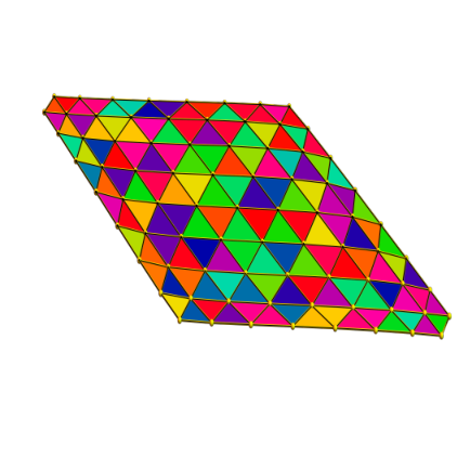
Lets look at some discrete manifolds with boundary. The case of an annulus is interesting as it is the simplest two-dimensional example with a non-trivial fundamental group.

3.13.
Example: for the dunce hat with vertices, where ,
we have
.
3.14.
For complete graphs , where , we have also because all eigenvalues of are either or .
3.15.
For a -spheres, we have . The torsion is
This simplifies with McKean-Singer to
We have as the number spanning trees in and as the number of spanning trees in .
Conjecture 1.
.


3.16.
Given an integer , we can ask for which is the expectation of Torsion on the probability space of Erdös-Rényi Graphs with vertices. This is difficult as we do not know already the expected Betti numbers . For now, we can just make experiments.
3.17.
The graph complement of cyclic graphs is interesting for various reasons
[16]. We measure for the numbers
.
and for the complements of linear path graphs
. We understand here the cases when is contractible in which case we have .
We have not yet figured out whether there is a formula for all these rational numbers.
4. Remarks
4.1.
Looking at graphs is almost equivalent than to look for finite abstract simplicial complexes. Any graph defines a simplicial complex, the Whitney complex and any finite abstract simplicial complex defines a graph given by incidence. The language of graphs is more approachable as we are familiar with graphs and networks like street or subway networks or family trees early on, while simplicial complexses already involve the concept of sets. Simplicial complexes are amazing too [14].
4.2.
is the squared super determinant of the chain complex. The notion of a determinant of a chain complex has been put forward in [6]. Since is a combinatorial notion and defined for any finite simple graph and not only if is a discrete manifold or evaluated in some limiting cases, we do not take the root . This allows us to stay rational.
4.3.
The manifold case needs analysis: the Ray-Singer determinant of a manifold defined by analytically continued Minakshisundaram-Pleijel zeta functions which can be defined using heat kernels. This requires assumptions or the “magic hand waving” of a jedi assuring that the pole singularities which might occur for the individual zeta functions cancel at [25]. At least initially, Ray-Singer had to make strong assumptions on the cohomology of the manifold.
4.4.
In the case of the circle for example, where , we have the eigenvalues of the Dirac operator with eigenvectors . for . This shows with the Riemann zeta function
we have included the factor is there because the spectrum of on -forms or on forms are both doubled. We have and . Therefore, . In order not to confuse the torsion notions, we call the square root of . This is now the volume (circumference) of the circle. The formula for the squared torsion is the continuum the equivalent of the formula for circular graphs . This example illustrates already in the simplest possible manifold case that analytic continuation issues occur.
4.5.
The Hodge Laplacian contains spectral information and much is certainly still hidden. The Betti numbers are the dimensions of the space of Harmonic -forms which according to Hodge are the ’th cohomology groups. (The observation that everything works just using linear algebra in the discrete seems first have been done by [4]). The fact that the spectral data define analytic data in the form of zeta functions and so lots of other quantities will certainly lead to more interesting quantities like the roots of the zeta function.
4.6.
The McKean-Singer symmetry for implies , pairs the non-zero eigenvalues of even and odd forms and immediately implies the McKean Singer relation which is a consequence of the fact that the Dirac operator produces this super-symmetry relation or spectral symmetry between even and odd forms. The simplest kind of super symmetry is the existence of a self-adjoint with and . This implies that if we have so that pairs eigenvectors. The matrix maps non-Harmonic eigenvectors of on even forms to eigenvectors on odd forms and vice versa.
4.7.
If is contractible, there is only one harmonic -form, the constant function. Let be the matrix obtained from by deleting the first row and first column. In the contractible case is invertible. We can write as a direct sum of the even-dimensional blocks and odd-dimensional blocks. The McKean-Singer relation can be rephrased using usual determinants
4.8.
By writing the determinant as a sum of permutations, we hope to have a pairing between these elements, if the graph is contractible. How would such a pairing look like? Can we pair every permutation of the simplices with a permutation of the simplices of . If that would be the case, we could try to get a pairing between rooted versions and get analytic torsion.
4.9.
We also expect that we can in the case of the truncated (called ), write for some complex . Longer shot: by building up the complex, we can always pair a positive new eigenvalue with an even simplex and one with an odd simplex. This pairing of simplices can give us a pairing of permutations. Now we would have to show that the product of the values are the same.
4.10.
An other corollary is that if is triangle free, then and since we have counts the number of rooted trees in G and counts the number of trees in . In general, in the contractible case, is a square.
4.11.
Remark. For practical reasons, we always assume that a sphere has the property that removing one point makes it contractible. (Unlike “homotopic to 1“ which is an NP complete task, “contractible” can be checked fast. Inductively, a graph is called contractible, if there exists a vertex such that and are both contractible. The induction assumption is that is contractible.)
4.12.
In general, if has a non-trivial cohomology or even non-trivial homotopy groups, things get more complicated. Analytic torsion is not invariant under Barycentric refinement, nor invariant under homotopy deformations even if rescaled. The first case to look at are deformed spheres. We see there that the formula for spheres has to be modified. Only the volume of the original underlying d-sphere matters. It is somehow a volume of a cohomology class.
4.13.
For a homotopy deformed -sphere coming from an actual -sphere , the volume of matters. Here are small dimensional examples: For a homotopy deformed circle coming from a sphere that . But this formula is already false if we add additional triangles.
4.14.
In the -dimensional case, we have invariance if we add lower dimensional parts. But adding three dimensional part directly does not work. For a homotopy deformed 2-sphere coming from a sphere that .
4.15.
We experimented also with deformations of 3-spheres: we see that for a homotopy deformed 3-sphere coming from a 3-sphere we have . But only as long as the deformed part intersects in lower dimensional parts.

4.16.
How do we get in general torsion from combinatorial data of ? In general this is not yet solved. Data can include the f-vector as well as the lengths of minimal non-contractible spheres embedded in . The following computation illustrates the effect of the fundamental group: if has no triangles and is homotopic to a bouquet of spheres with loops, then .
4.17.
We have tried to get relations for various products or sums or graph operations. We are also in interested in how depends on algebraic operations. An easy case is when are disjoint union of graphs. In that case
4.18.
We have seen that for some triangulations of the 2-torus, we have but that for others, it is not.
4.19.
Interestingly, there is also the following observation which we can not prove yet for the Shannon product of two circles.
Conjecture 2.
independent of .
4.20.
For example, for , a graph with Euler characteristic
and Betti vector (it is homotopic to a 2-torus),
the Hodge determinants are
,=
,
,
,
. This leads to .
The Dirac determinants are
, , .
This leads again to .
4.21.
For the homotopy cylinders we measure
Conjecture 3.
.
4.22.
But things get more complicated even if is contractible. If is the
wheel graph with vertices, then we see
, ,
, ,
suggesting
Conjecture 4.
.
If is the linear graph with vertices, we see
Conjecture 5.
.
4.23.
Cayley’s formula tells that the number of rooted -dimensional trees in a complete graph satisfies . More generally, we have
Lemma 2 (Generalized Cayley tree formula).
For the Hodge blocks: for and for .
For the Dirac blocks: for all .
This immediately implies:
Corollary 5.
Proof.
We can see this for the Hodge blocks
The identity could be seen by differentiating and setting . Easier is to see it for the Dirac blocks
which is ∎
4.24.
In order to prove that is a valuation in the contractible case. we want to interpret is a geometric quantity which satisfies the counting property: .
4.25.
Every finite simple graph defines its Whitney complex and every finite abstract simplicial complex defines the incidence graph and or are Barycentric refinements on the category of graphs or complexes. We insist to remain in a combinatorial setting and chose the language of graphs as this is much more intuitive. This also follows early topologists like Whitney, Alexandroff or Hopf, we like to think in terms of graphs (Gittergerüste) rather than finite set of sets or geometric realizations. The later leaves combinatorics and requires astronger axiom system ZFC. When doing finite combinatorics, we do not need the infinity axiom. It is also pedagogically simpler as what we do here is accessible to anybody who has seen matrices, eigenvalues and determinants in linear algebra. Simplicial complexes, CW complexes require more mathematical maturity.
4.26.
Our geometric point of view is to see a graph as a geometric model of a continuum like a compact Riemannian manifold . The graph naturally comes with a geodesic metric and recovers differential geometric notions like tensors. Fundamentally, if we look at space, we only can observe a finite set of points as well as relations between these points given by an equivalence relation that if two points are indistinguishable with a given accuracy. This define and the metric. If space is a compact Riemannian manifold and the number of points is finite but -dense with respect to some fixed non-standard small in an axiomatic framework like Nelson’s ZFC+IST or ZF+SPOT, we can recover the Riemannian metric from the geodesic graph metric.
4.27.
Not having any additional structure at first produces combinatorial problems which are not obscured by a particular choice of metric. The hope of course is always that some functional has interesting maxima or minima which somehow relate to physics. Natural functionals are Euler characteristic, Wu characteristic, average simplex cardinality [7], characteristic length [11]. Related to the pseudo determinant of the Dirac operator is torsion which is a super pseudo determinant of the Dirac operator.
4.28.
One of our initial motivations was the question of relating the spectrum of the Hodge Laplacian of a graph with the combinatorial data. A good starting point is the case of spheres, where we have Dehn-Sommerville relations involving the f-vector. Because of McKean-Singer, a natural quantity is the super determinant of Hodge operators. What is the geometric meaning if we weight the ’th term.
4.29.
When looking at the definition of analytic torsion, there is the strange power of in the ’th term. This disappears if one moves from the Hodge blocks to the Dirac blocks . Analytic torsion becomes so a very natural quantity as it is just the super determinant of the Dirac operator or the square of the super determinant of chain complex defined by .
4.30.
We made our first experiments with when writing [10] and experimented with analytic torsion in the summer of 2015 and saw then relations like for contractible graphs or . Being unable to prove the contractible case beyond the complete graph , we moved on to other projects and only returned to it in December 2021. We realized the proof of the 2-sphere case on December 25, 2021. We learned about the linear algebra relating the with from [1] only on January 4th, 2022. We found then also the appendix of [6], which introduces the determinant of a chain complex.
4.31.
The linear algebra switching from Hodge blocks to Dirac blocks is extremely important as it makes it clear why analytic torsion is such a natural quantity. We defined it as the square of the determinant of a chain complex. Just because we like to work with rational numbers and not square roots, we continued to work with the squared analytic torsion. When doing experiments, we see for example for the octahedron graph the torsion . If we would do the experiments with the square root, we would see and the connection to the -vector would have been obscures. Taking the rational numbers instead of the square roots looks like a small matter, but it was essential when investigating the matter experimentally.
4.32.
As the above remarks have indicated, there are lots of open questions. We see that for discrete manifolds that analytic torsion also depends on topology. A good start for further investigation is to see how torsion for -manifolds depends on the structure of the manifold. For homotopy tori obtained by taking the Shannon product of with , we always get . The graph is three dimensional in nature with the same number of of vertices and tetrahedra .
4.33.
Already Ray and Singer already suggested to study the analytic torsion for other differential complexes and not only the Euler complex. We can look at it for Wu characteristic , where the sum is over all pairs of complete sub-graphs of which have a non-empty intersection and where . Unlike Euler characteristic which is a homotopy invariant, the Wu characteristic is not. For discrete manifolds with -manifold boundary, it satisfies .
4.34.
The second order analogue of the -vector is the -matrix matters which counts the number of intersections of simplices with simplices. The second order analytic torsion is
where are the blocks of the Laplacian .
We see that for even dimensional spheres and for odd-dimensional spheres . We also see that for contractible graphs the situation is more subtle. We see that .
4.35.
Historically torsion was first considered for 3-manifolds by Reidemeister and was then extended by Franz to higher dimensions. It originally involved a representation of a group acting on the manifold. Torsion usually is defined for manifolds with trivial cohomology but equipped with a metric or with a unitary representation of the fundamental group. When considered for Riemannian manifolds, it involves also the volume.
4.36.
The pioneering papers are not so easy to read. Reidemeister torsion and analytic torsion were identified in [24, 3]. What we do here is much more elementary. Analytic torsion for graphs and more generally for any finite differential complex given by a finite sequence of derivative matrices only involves familiar linear algebra and is defined for arbitrary graphs or finite abstract simplicial complexes without additional structure. Especially, we never actually need even to involve the continuum. The pseudo determinant is a product of eigenvalues but it is also an entry in the characteristic polynomial defined by an integer matrix and so computable as an integer without detour over eigenvalues. Analytic torsion is a rational number explicitly computable in polynomial time from the simplicial complex (finding the Whitney complex can be costly as finding cliques in a graph in general is NP complete).
4.37.
The pioneering paper [5] which considers a cover of a topological complex for which all Betti numbers with respect to some field are zero but where one still can have a non-trivial fundamental group. Examples are lense spaces. Franz then looks at basis changes for which the determinant is in a fixed multiplicative subgroup of the field . Also [22] which is one of the later accounts of De Rham on torsion defines it for a group of units acting as automorphisms on a cellular complex.
4.38.
Milnor was one of the first, who picked up torsion, where de Rham left off. In [17], torsion was used to construct two manifolds with boundary which are not diffeomorphic, even so the interiors are diffeomorphic. Following Reidemeister, Franz and mostly de Rham one can define the torsion of a CW-complex equipped with a discrete group action so that has only finitely many cells. Given also a multiplicative homomorphism from to a commutative ring so that all the equivariant homologies are zero. Then torsion is defined as a unit in .
4.39.
[18] summarizes the beginnings: in 1935, Reidemeister [20], Franz [5] and de Rham [21] introduced the concept of ”torsion” for certain finite simplicial complexes . (…) it is a kind of determinant which describes the way in which the simplexes of are fitted together with respect to the action of the fundamental group. (…) In 1950, J. H. C. Whitehead defined the ”torsion” of a homotopy equivalence between finite complexes. This is a direct generalization of the Reidemeister [20], Franz, and de Rham concept; but is a more delicate invariant.
4.40.
For compact oriented Riemannian manifolds , the Ray-Singer torsion of is defined using the Ray-Singer determinant [19] which was introduced in 1971. They first refer to the Reidemeister-Franz torsion as a function of certain representations of the fundamental group and then introduce analytic torsion then state if is simply connected. The definition of uses zeta regularized determinants and only considered for odd dimensional manifolds as it is zero in the even dimensional case. In their definition of analytic torsion, [19] take a representation of the fundamental group by orthogonal matrices and differential forms with values in the associated vector bundle. They assume that the Laplacian has no zero eigenvalue so that the zeta function is analytic at allowing the definition. For modern approaches, see [2, 1].
4.41.
The zeta function of the ’th Laplacian of a manifold can be written as
because . The zeta function is analytic except for some poles. Then is defined as and analytic torsion as before. As pointed out in [25], the individual determinants are not always defined as can be pole, but magically, the various poles cancel. It goes without saying that computing the torsion for a given manifold using the definitions is almost impossible as we can not compute the eigenvalues explicitly. For a general manifold, one has to be in a situation, where the heat kernel asymptotic are known.
4.42.
We can also look at the zeta function in the discrete case. The Hodge block zeta function of the hodge defines a Hodge zeta function which is not interesting as by McKean-Singer, this is always constant zero. However, we can define the super Hodge zeta function of a graph as
which now the property that
4.43.
Much more natural is the Dirac zeta function
which again satisfies


4.44.
If is a finite simple graph, let denote the set of complete sub-graphs in . The union is a finite set of sets which is closed under the operation of taking non-empty subsets. It is a finite abstract simplicial complex. If is the cardinality of then is the -vector of . The integer is the maximal dimension and is the clique number. The integer is the number of simplices in . We fix a basis by assuming each to be ordered. The Dirac operator is a matrix. It depends on the given order but changing the order imposed on a simplex just produces an orthogonal change of basis.
4.45.
Even so we work with real matrices we write for the transpose of a matrix . The Dirac operator always is singular because the Hodge Laplacian is. If denotes the exterior derivative from -forms to -forms, then is a matrix. The Dirac block is a matrix and is essentially isospectral to which is a matrix. We can extend and to matrices so that they are matrices.
4.46.
This produces the Dirac columns , which is a matrix. Now, is a matrix . The matrix is an matrix which is essentially isospectral to . It is a block diagonal matrix which is zero everywhere except for the blocks and . We see .
4.47.
Define pseudo super determinant of as
Compare with the super determinant
4.48.
Lemma 3 (Key lemma).
Proof.
This product telescopes appears in the nominator and ∎
Corollary 6.
b) .
c) .
, , , . The Dirac determinant vector is is , , . The analytic torsion is . This is the same than .

4.49.
If is the Dirac operator of a graph . It is an matrix. Let denote the -matrix in which the first row and first column are deleted. The following lemma explains the factor appearing in the torsion of contractible graphs or spheres. It is a direct consequence of the classical matrix tree theorem.
Lemma 4 (Shaving Dirac A).
Let be defined from as above, then
a)
b)
Proof.
Since the first Dirac block agrees with the
Kirchhoff matrix and
where is the matrix in which the first row
and column are deleted. For all , the determinant
is the number of spanning trees rooted at the vertex .
The number is the number of spanning trees in the graph.
To get a), note that and
that the matrices are not affected by shaving off the first row and column.
To get b), we use that .
∎
4.50.
The dual story is when shaving away the last row and column of . Let the Dirac operator in which the last row and last column are deleted. The next lemma explains the factor appearing in torsion of spheres. Also this can be seen as a consequence of the matrix tree theorem.
Lemma 5 (Shaving Dirac B).
If is a d-sphere, and let be defined as above from , then
a)
b) if is even.
c) if is odd.
4.51.
This is in general false. We need the last Betti vector to be . But it holds for torus graphs.
4.52.
So, in order to prove the result, we replace with in the contractible case and replace with , the matrix in which the entire boundary has been shaved away. Let us introduce a new functional for contractible graphs
and for spheres:
Now everything boils down to
Lemma 6.
For spheres or contractible spaces, we have .
Proof.
For spheres and contractible spaces we have an interpretation as trees and so a Meyer-Vietoris valuation formula: . We can show this by induction. We can build up contractible graphs from smaller contractible graphs. We can also build d-spheres by gluing two d-balls (which are contractible) in such a way that is a -sphere. The reason for the formula is that now tells that there is a balance between even trees and odd trees. ∎
4.53.
We plan to follow up on the symmetry between even and odd trees in a future work. There is more to say about the duality of higher dimensional spanning trees in spheres.
References
- [1] U. Bunke. Lectures on analytic torsion. Lecture notes, Uni Regensburg, 2015.
- [2] D. Burghela, L. Friedlander, T. Kappeler, and P. McDonald. Analytic and Reidemeister torsion for representations in finite type Hilbert modules. Geom. Funct. Anal., pages 751–859, 1996.
- [3] J. Cheeger. Analytic torsion and the heat equation. Annals of Mathematics, 109:259–321, 1979.
- [4] B. Eckmann. The Euler characteristic - a few highlights in its long history. In Mathematical Survey Lectures: 1943-2004, 1999.
- [5] W. Franz. Über die Torsion einer Überdeckung. J. für reine und angew. Math., pages 245–254, 1935.
- [6] I.M. Gelfand, M.M. Kapranov, and A.V. Zelevinsky. Discriminants, Resultants, and Multidimensional Determinants. Springer, 1994.
- [7] O. Knill. The average simplex cardinality of a finite abstract simplicial complex. https://arxiv.org/abs/1905.02118, 1999.
- [8]
O. Knill.
An integrable evolution equation in geometry.
http://arxiv.org/abs/1306.0060, 2013. - [9]
O. Knill.
Isospectral deformations of the Dirac operator.
http://arxiv.org/abs/1306.5597, 2013. - [10] O. Knill. A Cauchy-Binet theorem for Pseudo determinants. Linear Algebra and its Applications, 459:522–547, 2014.
- [11]
O. Knill.
Characteristic length and clustering.
http://arxiv.org/abs/1410.3173, 2014. - [12]
O. Knill.
Gauss-Bonnet for multi-linear valuations.
http://arxiv.org/abs/1601.04533, 2016. - [13]
O. Knill.
The cohomology for Wu characteristics.
http://arxiv.org/abs/1803.06788, 2017. - [14]
O. Knill.
The amazing world of simplicial complexes.
https://arxiv.org/abs/1804.08211, 2018. - [15]
O. Knill.
Dehn-Sommerville from Gauss-Bonnet.
https://arxiv.org/abs/1905.04831, 2019. - [16] O. Knill. Graph complements of circular graphs. https://arxiv.org/abs/2101.06873, 2021.
- [17] J. Milnor. Two complexes which are homeomorphic but combinatorially distinct. Annals of Mathematics, 74:575–590, 1961.
- [18] J. Milnor. Whitehead torsion. Bull. Amer. Math. Soc., 72:358–426, 1966.
- [19] D.B. Ray and I.M. Singer. R-torsion and the laplacian on riemannian manifolds. Advances in Mathematics, 7:145–210, 1971.
- [20] K. Reidemeister. Homotopieringe und Linsenräume. Hamburger Abhandlungen, pages 102–109, 1935.
- [21] G. De Rham. Sur les complexes avec automorphisms. Comment. Math. Helv., 12:191–211, 1939.
- [22] G. De Rham. Torsion d’un complex a automorphismes. In S. Maumary G. De Rham and M.A. Kervaire, editors, Torsion et Type Simple d’Homotopie, pages 13–36, 1967.
- [23] K.G.C. Von Staudt. Geometrie der Lage. Nuernberg, 1847. page 21.
- [24] W. Müller. Analytic torsion and r-torsion of riemannian manifolds. Annals of Mathematics, 28:233–305, 1978.
- [25] E. Witten. Isadore Singer’s Work on Analytic Torsion. CMSA talk on April 6, 2021, 2021.