跳到论文正文
W Papers独立论文阅读器 arXiv:2201.09286 论文正文 计算阅读时间 · 0%
引用这篇论文根据当前论文元数据生成,正式投稿前建议核对。


License: arXiv.org perpetual non-exclusive license
arXiv:2201.09286v2 [cs.CV] 21 Feb 2022
 

How to scale hyperparameters for quickshift image segmentation


Damien Garreau

Université Côte d’Azur, Inria, CNRS, LJAD, France

Abstract

Quickshift is a popular algorithm for image segmentation, used as a preprocessing step in many applications. Unfortunately, it is quite challenging to understand the hyperparameters’ influence on the number and shape of superpixels produced by the method. In this paper, we study theoretically a slightly modified version of the quickshift algorithm, with a particular emphasis on homogeneous image patches with i.i.d. pixel noise and sharp boundaries between such patches. Leveraging this analysis, we derive a simple heuristic to scale quickshift hyperparameters with respect to the image size, which we check empirically.

1 INTRODUCTION

Quickshift is a clustering algorithm, which is used in image processing to obtain superpixels. It proceeds by first computing a kernel density estimate at scale ksk_{s}, then connecting each pixel to the nearest neighbor with higher density. All connections further away than dmd_{m} are removed, and the superpixels are then defined as the connected components of the resulting graph. Proposed by Vedaldi and Soatto 2008 as an efficient way to approximate the celebrated mean shift algorithm (Cheng 1995; Comaniciu and Meer 2002), the algorithm also appears in Rodriguez and Laio 2014. Together with SLIC (Achanta et al. 2012), compact watershed (Neubert and Protzel 2014), and Felzenszwalb (Felzenszwalb and Huttenlocher 2004), it is often used as a preprocessing step in more complex computer vision tasks such as image compression (Ryu et al. 2014) or semantic segmentation (Zhang et al. 2020). In the field of interpretability, quickshift is used as a default step when using LIME for images (Ribeiro et al. 2016), in order to create interpretable features.

Refer to caption
Figure 1: Segmentation of an image with quickshift with default hyperparameters (ks=5k_{s}=5, dm=10d_{m}=10). The superpixels are marked in yellow thick lines. The area inside the red rectangle is split up in 5656 superpixels despite being quite homogeneous.

In these applications, the number of superpixels produced by quickshift can be quite critical. For instance, in the case of LIME, the number of superpixels corresponds to the dimension of the linear model trained later on by the method (Garreau and Mardaoui 2021). Unfortunately, there is no way to know in advance the number of superpixels produced by quickshift as a function of the two main hyperparamters: ksk_{s} and dmd_{m}, in contrast for instance with SLIC. This can be particularly troublesome, in particular if the image at hand contains large, flat portions, where it is known that quickshift oversegments (see Figure 1). In contrast, boundaries between patches of different colors are seemingly always well-identified.

1.1 Summary of the paper

In this paper, we provide quantitative insights on the relationship between ksk_{s} and dmd_{m}, the two main hyperparameters of the method, and the number of superpixels produced when running the algorithm with this choice of hyperparameters. Our main theoretical contribution is the study of a modified version of quickshift on flat regions of the image. In that case, we show that this algorithm will find in average 𝒜/B⁡(ks,dm)\mathcal{A}/B(k_{s},d_{m}) local maxima, where B⁡(⋅,⋅)B(\cdot,\cdot) is 22-homogeneous and 𝒜\mathcal{A} is the area of the flat region (Theorem 3.2). Empirically, we demonstrate that these findings extend to the number of superpixels found by quickshift in real images. This yields the following heuristic: for a given image, multiplying ksk_{s} or dmd_{m} by κ\kappa will roughly divide the number of superpixels by κ2\kappa^{2}. We also show how sharp boundaries between homogeneous patches are detected by quickshift (Theorem 4.1).

The paper is organized as follows: in Section 2, we recall the detailed operation of quickshift. Section 3 contains the analysis for the flat portions, Section 4 for boundaries. Only sketches of the proofs are provided, the complete version of the proofs can be found in the Appendix. Finally, we show some experimental results in Section 5. All experiments are realized with the scikit-image implementation of quickshift and are publicly available.11 1 https://github.com/dgarreau/quickshift-scale

1.2 Related work

Density-based clustering algorithms proceed by first computing a density estimate (Parzen 1962), then either by looking at the level sets of the density or by hill-climbing. Quickshift belongs to the second category, and can be seen as a sample-based version of mean shift. This last method is analyzed in Arias-Castro et al. 2016, which shows that the updates converge to the correct gradient steps. Regarding quickshift, Jiang 2017 proves its consistency in the statistical sense, and gives the asymptotic size of ksk_{s} and dmd_{m} to recover the underlying density when the number of points grows to infinity. Since the result is asymptotic, it is difficult to use to pick ksk_{s} and dmd_{m} for a given image. Moreover, one of the main assumptions forbids the existence of flat regions in the theoretical analysis. A related analysis is proposed by Verdinelli and Wasserman 2018, with the same caveat. Also noting that density-based clustering algorithms tend to oversegment flat regions, Jiang et al. 2018 proposes a way to solve this problem, but this comes at the cost of computing cluster cores (Jiang and Kpotufe 2017) of the density estimate.

2 QUICKSHIFT: A REFRESHER

We now describe quickshift in more details, introducing notation along the way. In this description, we follow the scikit-image implementation (Van der Walt et al. 2014), which seems to be the most popular at the moment. In all the paper, we focus on a rectangular image ξ\xi, of size (0​p​t,0​p​t)(0pt,0pt). We denote the pixel positions by (i,j)∈I:=[0​p​t]×[0​p​t](i,j)\in I\vcentcolon=[0pt]\times[0pt], where [k]:={1,…,k}[k]\vcentcolon=\{1,\ldots,k\}. The pixels values are denoted by ξi,j∈ℝ3\xi_{i,j}\in\mathbb{R}^{3}. Strictly speaking, we work directly in the CIELAB space, though quickshift usually takes as input RGB images and converts them to the CIELAB space.

2.1 Density estimation

Quickshift relies on a Gaussian kernel density estimate which we denote by Pi,jP_{i,j}. The main idea is to see pixels as points in ℝ5\mathbb{R}^{5} (two space coordinates and three color coordinates). In practice, for each position pixel (i,j)(i,j), not all pixels of the image are considered to build this estimate, and only pixels (u,v)(u,v) close to (i,j)(i,j) are taken into account. More precisely, only (u,v)(u,v) inside

Ci,j:={(u,v)∈I, s.t. |i−u|∨|j−v|≤kw},C_{i,j}\vcentcolon=\{(u,v)\in I,\text{ s.t. }\left\lvert i-u\right\rvert\vee\left\lvert j-v\right\rvert\leq k_{w}\}\,, (1)

where kwk_{w} is a positive scale hyperparameter (called kernel width in the scikit-image implementation) are considered. Now we are able to define the density estimates, computed according to

Pi,j:=∑(u,v)∈Ci,je−(i−u)2−(j−v)2−‖ξi,j−ξu,v‖22​ks2,P_{i,j}\vcentcolon=\sum_{(u,v)\in C_{i,j}}\Exps^{\frac{-(i-u)^{2}-(j-v)^{2}-\left\lVert\xi_{i,j}-\xi_{u,v}\right\rVert^{2}}{2k_{s}^{2}}}\,, (2)

where ksk_{s} is a positive scale hyperparameter (called kernel size and equal to 55 by default in the scikit-image implementation). By default, kw=3​ksk_{w}=3k_{s}, an assumption that we will always make from now on, though it is straightforward to adapt our analysis for another fixed kwk_{w}. Finally, some i.i.d.​ 𝒩⁡(0,σ02)\Gaussian\left(0,\sigma_{0}^{2}\right) noise is added on each Pi,jP_{i,j} to break eventual ties (with σ0=10−5\sigma_{0}=10^{-5}). This procedure is described in Algorithm 1. The scikitlearn also has a ratio hyperparameter, allowing to adjust the importance of the pixel values with respect to the pixel positions. We do not consider this hyperparameter in our analysis, since it simply amounts to multiplying the pixel values by a positive constant, which does not change anything for flat regions.

Given (i,j)∈I(i,j)\in I, let us define for all (u,v)∈Ci,j(u,v)\in C_{i,j}

Xu,v:=exp⁡(−‖ξi,j−ξu,v‖22​ks2)⋅δu,v,X_{u,v}\vcentcolon=\Exp\left(\frac{-\left\lVert\xi_{i,j}-\xi_{u,v}\right\rVert^{2}}{2k_{s}^{2}}\right)\cdot\delta_{u,v}\,, (3)

where

δu,v:=exp⁡(−(i−u)2−(j−v)22​ks2).\delta_{u,v}\vcentcolon=\Exp\left(\frac{-(i-u)^{2}-(j-v)^{2}}{2k_{s}^{2}}\right)\,. (4)

With these notation in hand, we see that

∀(i,j)∈I,Pi,j=∑(u,v)∈Ci,jXu,v,\forall(i,j)\in I,\quad P_{i,j}=\sum_{(u,v)\in C_{i,j}}X_{u,v}\,,

and already we can spot two major difficulties in our analysis. The first is that, even if we assume the ξi,j\xi_{i,j}s to be independent random variables, the Xu,vX_{u,v}s are not, and as a consequence the Pi,jP_{i,j}s are not independent. As a consequence, looking at statements involving several Pi,jP_{i,j}s is very challenging. Our approach in Section 3 will be to simplify the problem by reducing PP to its main component QQ, using standard tools from the theory of UU-statistics. The independence of the Qi,jQ_{i,j}s makes them much more convenient to work with. Our main challenge will be to show that nothing of value is lost when making this approximation.

Second, let us define Im​(kw)I_{m}(k_{w}) the set of points of II that are further than kwk_{w} away from the border of the image. By definition, for all (i,j)∈Im​(kw)(i,j)\in I_{m}(k_{w}), Ci,jC_{i,j} is the set of points contained in a square of side 2​kw+12k_{w}+1 centered in (i,j)(i,j) (see Figure 4). The picture is more complicated near the borders of the image: for instance, right next to the border, Ci,jC_{i,j} has roughly half its size, which drastically lowers the density estimates near the border, even in simple cases. As we will see in Section 4, this has non-trivial consequences. Note that some implementations do normalize Eq. (2) (for instance in the GPU implementation of Fulkerson and Soatto 2010), which removes this problem.

Algorithm 1 Density estimation.
0:  Image ξ∈ℝ0​p​t×0​p​t\xi\in\mathbb{R}^{0pt\times 0pt}, kernel size ksk_{s}.
1:  Set: kw←3​ksk_{w}\leftarrow 3k_{s}
2:  Initialize: P∈ℝ0​p​t×0​p​tP\in\mathbb{R}^{0pt\times 0pt}
3:  for (i,j)∈I(i,j)\in I do
4:   Pi,j←0P_{i,j}\leftarrow 0
5:   for (u,v)∈Ci,j(u,v)\in C_{i,j} do
6:    Pi,j←Pi,j+exp⁡(−(i−u)2−(j−v)2−‖ξi,j−ξu,v‖22​ks2)P_{i,j}\leftarrow P_{i,j}+\Exp\left(\frac{-(i-u)^{2}-(j-v)^{2}-\left\lVert\xi_{i,j}-\xi_{u,v}\right\rVert^{2}}{2k_{s}^{2}}\right)
7:   end for
8:   Pi,j←Pi,j+𝒩⁡(0,σ02)P_{i,j}\leftarrow P_{i,j}+\Gaussian\left(0,\sigma_{0}^{2}\right)
9:  end for
10:  return PP

2.2 Graph construction

We now turn to the graph construction, the heart of the quickshift algorithm, which we describe for any array A∈ℝ0​p​t×0​p​tA\in\mathbb{R}^{0pt\times 0pt}. Intuitively, quickshift moves each pixel to the nearest neighbor with higher density. When this is no longer possible, we have found a local maximum of the density. Formally, quickshift produces a directed graph 𝒢0​(A)\mathcal{G}_{0}(A) with vertices II in the following way: first, all vertices are visited, and quickshift places an edge between (i,j)(i,j) and (u,v)∈Ci,j(u,v)\in C_{i,j} if two conditions are satisfied: (i) Ai,j<Au,vA_{i,j}<A_{u,v}, and (ii) (i−u)2+(j−v)2+‖ξi,j−ξu,v‖2(i-u)^{2}+(j-v)^{2}+\left\lVert\xi_{i,j}-\xi_{u,v}\right\rVert^{2} is minimal among all (u,v)∈Ci,j(u,v)\in C_{i,j} satisfying condition (i). Second, all edges between pixels with (55-dimensional) distance greater than dmd_{m} are removed from 𝒢0​(A)\mathcal{G}_{0}(A), where dmd_{m} is a positive hyperparameter called maximal distance in the scikit-image implementation and set to 1010 by default. Finally, the superpixels are defined as the connected components of 𝒢0​(A)\mathcal{G}_{0}(A). The graph construction is summarized in Algorithm 2.

Algorithm 2 Quickshift graph construction (following skimage implementation).
0:  Image ξ∈ℝ0​p​t×0​p​t\xi\in\mathbb{R}^{0pt\times 0pt}, kernel size ksk_{s}, maximum distance dmd_{m}, array A∈ℝ0​p​t×0​p​tA\in\mathbb{R}^{0pt\times 0pt}.
1:  set: kw←3​ksk_{w}\leftarrow 3k_{s}
2:  for (i,j)∈I(i,j)\in I do
3:   initialize: M←+∞M\leftarrow+\infty with same shape as Ci,jC_{i,j}
4:   for (u,v)∈Ci,j(u,v)\in C_{i,j} do
5:    d←(i−u)2+(j−v)2+‖ξi,j−ξu,v‖2d\leftarrow(i-u)^{2}+(j-v)^{2}+\left\lVert\xi_{i,j}-\xi_{u,v}\right\rVert^{2}
6:    if Ai,j<Au,vA_{i,j}<A_{u,v} and d≤dmd\leq d_{m} then
7:     Mu,v←dM_{u,v}\leftarrow d
8:    end if
9:   end for
10:   (u,v)←arg​min⁡M(u,v)\leftarrow\Argmin M
11:   G(i,j),(u,v)←1G_{(i,j),(u,v)}\leftarrow 1
12:  end for
13:  return GG

In definitive, we see quickshift as the application of the graph construction procedure given by Algorithm 2 to the density estimate obtained by Algorithm 1. That is, quickshift first computes PP by means of Algorithm 1 and then applies Algorithm 2 to A=PA=P. Other implementations exist, though they share the same basic ideas. For instance, the VLFeat library normalizes the Pi,jP_{i,j}s by 1/(2​π​ks)5+21/(2\pi k_{s})^{5+2}.

2.3 Computational complexity

A naive implementation of the density estimation step (Algorithm 1) requires a full pass on the image, and for each pixel a pass on Ci,jC_{i,j}. Therefore, the density estimation part of quickshift costs 𝒪⁡(0​p​t​0​p​t​kw2)\mathcal{O}\left(0pt0ptk_{w}^{2}\right). Regarding the graph construction (Algorithm 2), first one has to parse the image once again and look into the Ci,jC_{i,j} windows, which costs 𝒪⁡(0​p​t​0​p​t​kw2)\mathcal{O}\left(0pt0ptk_{w}^{2}\right). Subsequently, we need to find the connected components of a directed graph with 0​p​t⋅0​p​t0pt\cdot 0pt vertices and the same number of edges, which costs 𝒪⁡(0​p​t​0​p​t)\mathcal{O}\left(0pt0pt\right) (Hopcroft and Tarjan 1973). In definitive, the total computational cost is linear in 0​p​t0pt and 0​p​t0pt, and quadratic in kwk_{w}. This is something to consider when increasing the kwk_{w} hyperparameter. Finally, note that the dmd_{m} hyperparameter has no influence on the computational cost, though setting small values can lead to producing many superpixels. In particular, by the graph construction, all superpixels have geometric diameter smaller than dmd_{m}.

Refer to caption
Figure 2: Density estimation under Assumption 3.1 for a 50×5050\times 50 image with σ=1.0\sigma=1.0. Left: using the definition, Eq. (2); middle: using the Hájek projection, P^i,j\widehat{P}_{i,j}; right: using only the main term Qi,jQ_{i,j} (Eq. (5)). As predicted by Theorem 3.1, PP and QQ are close to each other, and so are the associated local maxima (in red). Of course, their number and exact positions can differ.

3 HOMOGENEOUS PATCHES

In this section, we focus on flat portions of the image. That is, subsets of II such that ξi,j\xi_{i,j} is approximately constant. As a simple model for this situation, we propose the following:

Assumption 3.1 (Flat image).

For all (i,j)∈I(i,j)\in I, the ξi,j\xi_{i,j} are i.i.d.​ 𝒩⁡(c,σ2​I3)\Gaussian\left(c,\sigma^{2}\Identity_{3}\right), where c∈ℝ3c\in\mathbb{R}^{3} is an arbitrary color and σ≤ks/5\sigma\leq k_{s}/5.

This assumption is a simple model of the random noise coming from an electronic sensor when photographing a mono-color item (see, e.g., Pratt 2001). Under this assumption, we derive an approximate expression for PP in Section 3.1, before introducing in Section 3.2 the modification of the quickshift algorithm that we investigate here. After precising the interplay between local maxima and superpixels in Section 3.3, we state our main result in Section 3.4.

3.1 A closer look at density estimation

Under Assumption 3.1, it is straightforward to compute the first moments of the Xu,vX_{u,v}, and by extension those of Pi,jP_{i,j}. Let us first define the normalization constant

Cp:=(ks2ks2+p​σ2)3/2.C_{p}\vcentcolon=\left(\frac{k_{s}^{2}}{k_{s}^{2}+p\sigma^{2}}\right)^{3/2}\,.

Then we show in the Appendix that 𝔼⁡[Pi,j]=C2​Δi,j\Expec\left[P_{i,j}\right]=C_{2}\Delta_{i,j}, where Δi,j:=∑(u,v)∈Ci,jδu,v\Delta_{i,j}\vcentcolon=\sum_{(u,v)\in C_{i,j}}\delta_{u,v}. As noted in Section 2, the Xu,vX_{u,v} are not independent. For instance, we show in the Appendix that Cov⁡(Xu,v,Xu′,v′)\mathrm{Cov}(X_{u,v},X_{u^{\prime},v^{\prime}}) is always positive under 3.1. Nonetheless, a careful reading of Eq. (3) reveals that ξi,j\xi_{i,j} draws all values of the density estimate. More precisely, ξi,j\xi_{i,j} is present in all the Xu,vX_{u,v} (there are 𝒪⁡(ks2)\mathcal{O}\left(k_{s}^{2}\right) of them), whereas each other individual Xu,vX_{u,v} is only present one time. Therefore, when ksk_{s} is large, we expect Pi,jP_{i,j} to behave roughly as its conditional expectation with respect to ξi,j\xi_{i,j} for a given (i,j)(i,j), which is given by

Qi,j:=C1⋅exp⁡(−‖ξi,j−c‖22​(ks2+σ2))⋅Δi,j.Q_{i,j}\vcentcolon=C_{1}\cdot\Exp\left(\frac{-\left\lVert\xi_{i,j}-c\right\rVert^{2}}{2(k_{s}^{2}+\sigma^{2})}\right)\cdot\Delta_{i,j}\,. (5)

We formalize this intuition by the following:

Theorem 3.1 (Pi,jP_{i,j} is close to Qi,jQ_{i,j}, w.h.p.).

Assume that 3.1 holds. Suppose furthermore that ks≥5k_{s}\geq 5. Let (i,j)∈Im​(kw)(i,j)\in I_{m}(k_{w}). Then, for any ε>0\varepsilon>0,

ℙ⁡(|Pi,j−Qi,j|>ε)≤71​σ2ε2.\Proba\left(\left\lvert P_{i,j}-Q_{i,j}\right\rvert>\varepsilon\right)\leq\frac{71\sigma^{2}}{\varepsilon^{2}}\,.

The main consequence of this result is that one can study Qi,jQ_{i,j} instead of Pi,jP_{i,j} when σ\sigma is small, at least for a fixed (i,j)∈Im​(kw)(i,j)\in I_{m}(k_{w}). We refer to Figure 2 for an illustration. Theorem 3.1 is the main motivation to study the graph construction step of quickshift on QQ instead of PP. Of course, looking at the graph construction implies looking simultaneously to several Pi,jP_{i,j}s, a case which is not covered by Theorem 3.1. We conjecture that a uniform bound for all (i,j)∈Im​(kw)(i,j)\in I_{m}(k_{w}) exists, though a straightforward approach via a union bound argument does not yield a satisfying bound.

Sketch of the proof of Theorem 3.1. Following Van der Vaart 2000, the key idea of the proof is to compute the Hájek projection of Pi,jP_{i,j} onto the set of random variables ξu,v\xi_{u,v}, (u,v)∈I(u,v)\in I to capture the influence of each of the ξu,v\xi_{u,v}. We then show that the projection onto ξi,j\xi_{i,j}, that is, Qi,jQ_{i,j}, is the most prominent one. We start by computing the Hájek projection of Pi,jP_{i,j}, which boils down to Gaussian integral computations under Assumption 3.1, and we find, ∀(i,j)∈I\forall(i,j)\in I,

P^i,j=Qi,j+C1​∑(u,v)∈Ci,j(u,v)≠(i,j)(e−‖ξu,v−c‖22​(ks2+σ2)−(ks2+σ2ks2+2​σ2)32)​δu,v\widehat{P}_{i,j}=Q_{i,j}+\,C_{1}\!\!\!\!\!\!\!\sum_{\begin{subarray}{c}(u,v)\in C_{i,j}\\ (u,v)\neq(i,j)\end{subarray}}\left(\Exps^{\frac{-\left\lVert\xi_{u,v}-c\right\rVert^{2}}{2(k_{s}^{2}+\sigma^{2})}}-\left(\tfrac{k_{s}^{2}+\sigma^{2}}{k_{s}^{2}+2\sigma^{2}}\right)^{\frac{3}{2}}\right)\!\delta_{u,v} (6)

We are then able to show that Pi,jP_{i,j} and P^i,j\widehat{P}_{i,j} have similar variances when ksk_{s} is large enough. More precisely,

|Var⁡(P^i,j)Var⁡(Pi,j)−1|≤45​ks2.\left\lvert\frac{\Var(\widehat{P}_{i,j})}{\Var\left(P_{i,j}\right)}-1\right\rvert\leq\frac{4}{5k_{s}^{2}}\,.

Therefore, an application of Theorem 11.2 in Van der Vaart 2000 yields:

ℙ⁡(|Pi,j−𝔼⁡[Pi,j]Var⁡(Pi,j)−P^i,j−𝔼⁡[P^i,j]Var⁡(P^i,j)|>ε)≤1ks2​ε2.\Proba\left(\left\lvert\frac{P_{i,j}-\Expec\left[P_{i,j}\right]}{\sqrt{\Var\left(P_{i,j}\right)}}-\frac{\widehat{P}_{i,j}-\Expec[\widehat{P}_{i,j}]}{\sqrt{\Var(\widehat{P}_{i,j})}}\right\rvert>\varepsilon\right)\leq\frac{1}{k_{s}^{2}\varepsilon^{2}}\,.

Let us define Ri,j:=P^i,j−Qi,jR_{i,j}\vcentcolon=\widehat{P}_{i,j}-Q_{i,j}, the rest term. Then we are able to show that Var⁡(Ri,j)≤σ2/4\Var\left(R_{i,j}\right)\leq\sigma^{2}/4. Thus, for any given (i,j)(i,j), when ksk_{s} is large enough and σ\sigma is small with respect to ksk_{s}, we can identify Pi,jP_{i,j} with P^i,j\widehat{P}_{i,j}, which in turn can be identified with Qi,jQ_{i,j}, concluding the proof of Theorem 3.1. ∎

Figure 3: A sample graph 𝒢⁡(P)\mathcal{G}(P) obtained by the running Algorithm 3 on the density estimate PP of an image of size 10×1510\times 15. Each arrow connects a pixel to the nearest pixel having a higher density estimate. The local maxima are marked in red: there is one such local maxima per connected component of 𝒢\mathcal{G}, as per Lemma 3.1.

3.2 Modified graph construction

We now present a slight modification in the graph construction. Namely, we remove the ‖ξi,j−ξu,v‖2\left\lVert\xi_{i,j}-\xi_{u,v}\right\rVert^{2} term from the distance computation (line 5 of Algorithm 2). Indeed, under Assumption 3.1, 𝔼⁡[‖ξi,j−ξu,v‖2]=𝒪⁡(σ2)\Expec[\left\lVert\xi_{i,j}-\xi_{u,v}\right\rVert^{2}]=\mathcal{O}\left(\sigma^{2}\right). Since the Euclidean distance term is 𝒪⁡(1)\mathcal{O}\left(1\right), the color difference term is negligible whenever σ\sigma is small or dmd_{m} is large, and there is little difference between the output of Algorithm 2 and 3. Of course, as soon as σ\sigma is of the order of magnitude of dmd_{m}, notable differences appear. In particular, Algorithm 3 tends to produce much more superpixels in this situation.

A key observation is that, when using this modified version of quickshift, the graph construction simplifies greatly: instead of looking for values of AA that are greater than Ai,jA_{i,j} inside Ci,jC_{i,j} and subsequently cut off all points with 55-dimensional distance greater than dmd_{m}, we can look directly for points in Ei,j:=Ci,j∩Di,jE_{i,j}\vcentcolon=C_{i,j}\cap D_{i,j}, where Di,jD_{i,j} is the set of points of II such that (i−u)2+(j−v)2≤dm\sqrt{(i-u)^{2}+(j-v)^{2}}\leq d_{m}. There are three possibilities for Ei,jE_{i,j}, depending on the relative position of kwk_{w} and dmd_{m}: we depict these three cases in Figure 4. We call 𝒢⁡(A)\mathcal{G}(A) this procedure, described formally in Algorithm 3 and illustrated in Figure 3.

To conclude this section, we want to emphasize that the core analysis of this paper concerns 𝒢⁡(Q)\mathcal{G}(Q), not 𝒢0​(P)\mathcal{G}_{0}(P) which is the output of the default implementation.

Refer to caption
Figure 4: Three possibilities for the lookout area of Algorithm 3. At a given (i,j)∈I(i,j)\in I (in red), the algorithm looks at the nearest neighbor with higher value in Ei,j=Ci,j∩Di,jE_{i,j}=C_{i,j}\cap D_{i,j} (solid blue line). The shape of the intersection depends on the interplay between ksk_{s} and dmd_{m}. For instance, the default choice ks=5k_{s}=5 and dm=10d_{m}=10 yields kw=15k_{w}=15, which is greater than dmd_{m}: we are in the disk case. This trichotomy remains when both ksk_{s} and dmd_{m} are multiplied by a constant factor.
Algorithm 3 Simplified quickshift graph construction.
0:  Image ξ∈ℝ0​p​t×0​p​t\xi\in\mathbb{R}^{0pt\times 0pt}, kernel size ksk_{s}, maximum distance dmd_{m}, array A∈ℝ0​p​t×0​p​tA\in\mathbb{R}^{0pt\times 0pt}.
1:  set: kw←3​ksk_{w}\leftarrow 3k_{s}
2:  for (i,j)∈I(i,j)\in I do
3:   (u,v)←(u,v)\leftarrow closest element of Ei,jE_{i,j} s.t. Ai,j<Au,vA_{i,j}<A_{u,v}
4:   G(i,j),(u,v)←1G_{(i,j),(u,v)}\leftarrow 1
5:  end for
6:  return GG

3.3 Counting superpixels

We now return to our main focus: counting the number of superpixels. For a given region RR of the image, we set KR​(A)K_{R}(A) the number of connected components of 𝒢⁡(A)\mathcal{G}(A) intersecting RR. It is challenging to investigate KR​(A)K_{R}(A) directly, and we rather study the number of local maxima:

Definition 3.1 (Local maximum).

Let A∈ℝ0​p​t×0​p​tA\in\mathbb{R}^{0pt\times 0pt} and (i,j)∈I(i,j)\in I. We say that (i,j)(i,j) is a local maximum of AA if ∀(u,v)∈Ei,j\forall(u,v)\in E_{i,j}, Ai,j>Au,vA_{i,j}>A_{u,v}.

We will use the notation NR​(A)N_{R}(A) to denote the number of local maxima of AA inside a given region RR. The main reason to study local maxima is that, on a global scale, there is an equivalence between the number of superpixels and the number of local maxima, as is demonstrated in Figure 3. This fact is formalized by our next lemma:

Lemma 3.1 (Connected components and local maxima).

Let 𝒢⁡(A)\mathcal{G}(A) be the directed graph produced by Algorithm 3 applied to an array A∈ℝ0​p​t×0​p​tA\in\mathbb{R}^{0pt\times 0pt}. Then to each connected component of 𝒢⁡(A)\mathcal{G}(A) corresponds a unique local maxima of AA in the sense of Definition 3.1.

In view of Lemma 3.1, we will now focus on NR​(A)N_{R}(A), which is a priori distinct from KR​(A)K_{R}(A). Indeed, when restricting ourselves to RR, it can happen that we miss the local maxima corresponding to the connected component intersecting with RR. Namely, only the trivial lower bound

NR​(A)≤KR​(A)N_{R}(A)\leq K_{R}(A)\, (7)

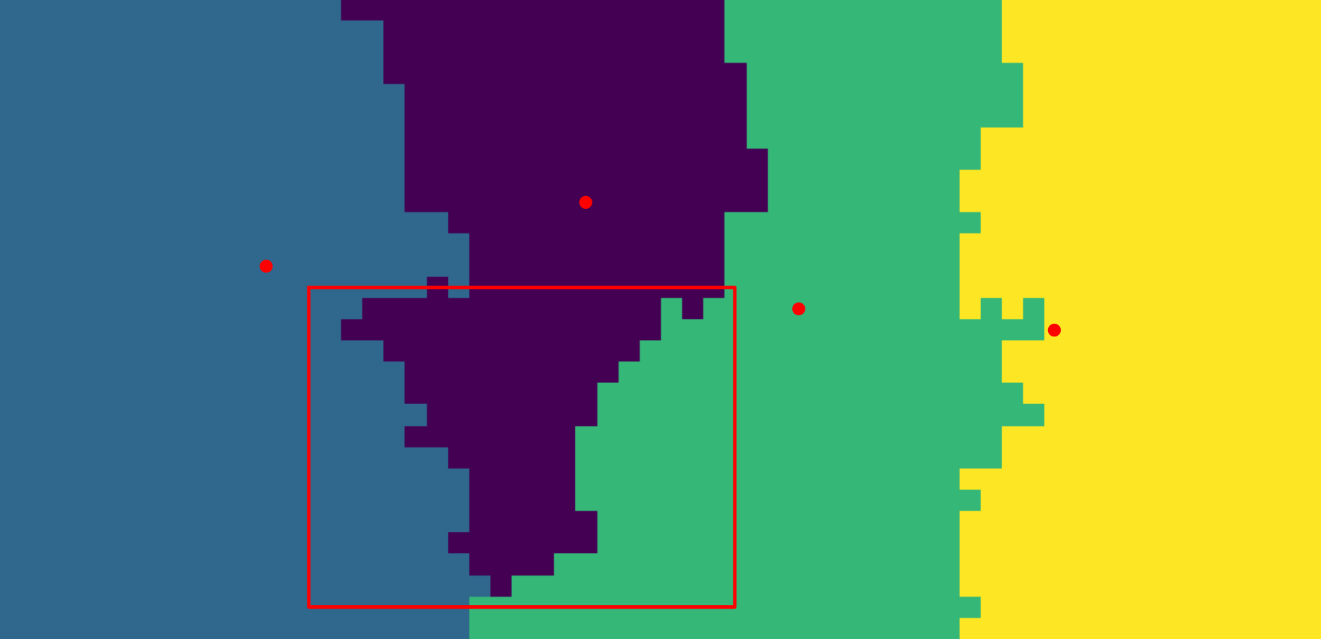
holds. There is no corresponding upper bound in the general case, since a rectangle can intersect many superpixels without containing any local maximum as depicted in Figure 5. Nevertheless, empirically, NR​(A)N_{R}(A) and KR​(A)K_{R}(A) are comparable for large regions (and the bound given by Eq. (7) is reasonably tight).
Refer to caption
Figure 5: The number of local maxima inside a part of the image does not always coincide with the number of superpixels intersecting this area. In this example, RR is a rectangle with boundaries marked in red. The number of local maxima inside RR is NR​(A)=0N_{R}(A)=0, whereas the number of superpixels intersecting RR is KR​(A)=3K_{R}(A)=3.
Refer to caption
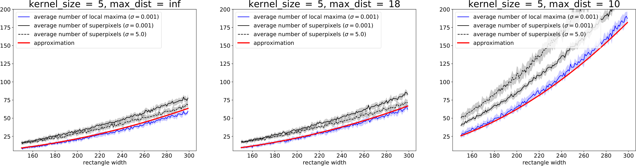
Figure 6: Evolution of the number of superpixels created by quickshift under Assumption 3.1. For each input shape, we run quickshift on ten images and count the number of local maxima and the number of superpixels in a rectangular patch far from the border of the image. We see that, when σ\sigma is small, the prediction of Theorem 3.2 (in red) is close to the empirical number of local maxima (in blue). Moreover, the number of local maxima coincides roughly with the number of superpixels (in black). When σ\sigma increases, as expected, this link weakens but we still observe a quadratic dependency in the size of the rectangle. The three choices of (ks,dm)(k_{s},d_{m}) correspond to the three different configurations (square, rounded square, and disk).

3.4 Average number of local maxima in flat regions

We are now ready to state and prove the main result of this section.

Theorem 3.2 (Average number of local maxima).

Assume that 3.1 holds. Let R⊆IR\subseteq I be a rectangle of height hh and width ww at distance greater than 2​kw2k_{w} from the border. Then

𝔼⁡[NR​(Q)]={hw⋅(1π​dm2+𝒪⁡(1dm))​ if ​dm≤kwhw⋅(1π⁡(3​kw​dm−kw2−dm2)+𝒪⁡(1kw)) if ​kw<dm≤2​kwhw⋅(14​kw2+𝒪⁡(1kw))​ otherwise. \Expec\left[N_{R}(Q)\right]=\begin{cases}hw\cdot\left(\frac{1}{\pi d_{m}^{2}}+\mathcal{O}\left(\frac{1}{d_{m}}\right)\right)\text{ if }d_{m}\leq k_{w}\\ hw\cdot\left(\frac{1}{\pi(3k_{w}d_{m}-k_{w}^{2}-d_{m}^{2})}+\mathcal{O}\left(\frac{1}{k_{w}}\right)\right)\\ \phantom{blablablabkablabla}\text{ if }k_{w}<d_{m}\leq\sqrt{2}k_{w}\\ hw\cdot\left(\frac{1}{4k_{w}^{2}}+\mathcal{O}\left(\frac{1}{k_{w}}\right)\right)\text{ otherwise. }\end{cases}

The main consequence of Theorem 3.2 is the scale of NR​(Q)N_{R}(Q) with respect to (i) the size of RR, and (ii) the hyperparameters. In plain words, firstly, we find NR​(Q)N_{R}(Q) to be proportional to the area of RR: a flat, rectangular part of the image will contain twice as many superpixels if its size is multiplied by two. Secondly, whatever the relative position of ksk_{s} and dmd_{m} is, NR​(Q)N_{R}(Q) is (−2)(-2)-homogeneous in (ks,dm)(k_{s},d_{m}): doubling both ksk_{s} and dmd_{m} will approximately divide NR​(Q)N_{R}(Q) by four. We illustrate the validity of Theorem 3.2 with respect to the non-modified version of quickshift (Algorithm 2 running on PP) in Figure 6.

Proof of Theorem 3.2. The key of the proof is the following result, which is the main motivation for finding an i.i.d.​ approximation of PP:

Lemma 3.2 (Key lemma).

Let A∈ℝ0​p​t×0​p​tA\in\mathbb{R}^{0pt\times 0pt} be a random array such that the Ai,jA_{i,j} are i.i.d.​ with cumulative distribution function GG and associated density gg. Let R⊆IR\subseteq I. Define Ni,j:=#​Ei,jN_{i,j}\vcentcolon=\#E_{i,j}. Then the expected number of local maxima in RR produced by Algorithm 3 applied to AA is given by

𝔼⁡[NR​(A)]=∑(i,j)∈R1Ni,j.\Expec\left[N_{R}(A)\right]=\sum_{(i,j)\in R}\frac{1}{N_{i,j}}\,.

Note that, as a consequence, Theorem 3.2 is not limited to a rectangular area, though it is less convenient to state for a general shape.

Proof of Lemma 3.2. We first write NR​(A)N_{R}(A) as the sum of indicator that (i,j)(i,j) is a local maximum. Further,

𝔼⁡[NR​(A)]=𝔼⁡[∑(i,j)∈R𝟙∀(u,v)∈Ei,j⋆,Ai,j>Au,v]\displaystyle\Expec\left[N_{R}(A)\right]=\Expec\left[\sum_{(i,j)\in R}\mathds{1}_{\forall(u,v)\in E_{i,j}^{\star},\,\,A_{i,j}>A_{u,v}}\right]
=∑(i,j)∈Rℙ(∀(u,v)∈Ei,j⋆,Ai,j>Au,v),\displaystyle=\sum_{(i,j)\in R}\Proba\left(\forall(u,v)\in E_{i,j}^{\star},\,\,A_{i,j}>A_{u,v}\right)\,,

where we write Ei,j⋆E_{i,j}^{\star} short for Ei,j∖{(i,j)}E_{i,j}\setminus\{(i,j)\}. Let us condition with respect to Ai,jA_{i,j}. Using the i.i.d.​​ assumption on the Ai,jA_{i,j}s, by definition of the cumulative distribution function GG,

ℙ(∀(u,v)∈Ei,j⋆,Ai,j>Au,v|Ai,j)=G(Ai,j)Ni,j−1.\mathbb{P}\left(\forall(u,v)\in E_{i,j}^{\star},\,\,A_{i,j}>A_{u,v}\middle|A_{i,j}\right)=G(A_{i,j})^{N_{i,j}-1}\,.

Integrating the last display yields the result, since

∫G​(t)Ni,j−1​g​(t)​𝑑t=[G​(t)Ni,jNi,j]−∞+∞=1Ni,j.\displaystyle\int G(t)^{N_{i,j}-1}g(t)\,\mathrm{d}t=\left[\frac{G(t)^{N_{i,j}}}{N_{i,j}}\right]_{-\infty}^{+\infty}=\frac{1}{N_{i,j}}\,.

∎

Further, we see that the Qi,jQ_{i,j} are indeed i.i.d.​ if we are outside a band of width 2​kw2k_{w} from the border: here, Δi,j\Delta_{i,j} does not depend on (i,j)(i,j). Thus we can apply Lemma 3.2 to the random array QQ. Finally, it is just a matter of counting the number of points inside Ei,jE_{i,j}. For instance, let us assume that dm≤kwd_{m}\leq k_{w}. In that case, we have to count the number of lattice points inside a disk of radius dmd_{m}. This is known as the Gauss circle problem, and an immediate bound (due to Gauss himself) is Ni,j=π​dm2+𝒪⁡(dm)N_{i,j}=\pi d_{m}^{2}+\mathcal{O}\left(d_{m}\right). Summing over all pixels in RR yields the last result in Theorem 3.2. The other cases are similar and the details can be found in the Appendix. ∎

4 SHARP EDGES

In this short section, we focus on well-defined boundaries between homogeneous patches of the image. More precisely, we assume the following:

Assumption 4.1 (Bicolor image).

There exist j0∈[0​p​t]j_{0}\in[0pt], c1,c2∈ℝ3c_{1},c_{2}\in\mathbb{R}^{3} such that the ξi,j\xi_{i,j} are i.i.d. 𝒩⁡(c1,σ2​I3)\Gaussian\left(c_{1},\sigma^{2}\Identity_{3}\right) (resp. 𝒩⁡(c2,σ2​I3)\Gaussian\left(c_{2},\sigma^{2}\Identity_{3}\right)) on Iℓ:=[0​p​t]×{1,…,j0}I_{\ell}\vcentcolon=[0pt]\times\{1,\ldots,j_{0}\} (resp. Ir:=[0​p​t]×{j0,…,0​p​t}I_{r}\vcentcolon=[0pt]\times\{j_{0},\ldots,0pt\}), with σ≤ks/5\sigma\leq k_{s}/5.

In plain words, we consider a bicolor image with a vertical boundary at j0j_{0} between them and i.i.d.​ Gaussian noise as in Section 3. We refer to Figure 7 for a visual depiction.

Refer to caption
Figure 7: The bicolor setting described by Assumption 4.1. Here, c1c_{1} is a light blue and c2c_{2} a light red. The border between the two patches marked at j0j_{0} is in the middle of the image.

Note that we can also work under Assumption 4.1 to understand what happens at the border of a flat image: Let us consider (i,j)(i,j) a pixel near the boundary of the image. In that case, Ci,jC_{i,j} contains fewer points than in the center of the image since the square centered at (i,j)(i,j) “overflows” the image, and therefore the sum in Eq. (2) is missing some terms. Instead of thinking of Ci,jC_{i,j} as reduced, we can think of Ci,jC_{i,j} intersecting a color patch where ‖ξu,v−ξi,j‖\left\lVert\xi_{u,v}-\xi_{i,j}\right\rVert is very large for all (u,v)(u,v) in that patch. In that event, the corresponding terms in Eq. (2) vanish. Without further ado, we can state the main result of this section:

Theorem 4.1 (Increasing density estimates).

Assume that 4.1 holds. Assume further that ks≥5k_{s}\geq 5 and that ‖c1−c2‖≥3​ks\left\lVert c_{1}-c_{2}\right\rVert\geq 3k_{s}. Then, for any (i,j)∈Im∩Iℓ(i,j)\in I_{m}\cap I_{\ell} such that |j−j0|≤kw\left\lvert j-j_{0}\right\rvert\leq k_{w},

ℙ⁡(Pi,j>Pi,j+1)≥1−16​σ2.\Proba\left(P_{i,j}>P_{i,j+1}\right)\geq 1-16\sigma^{2}\,.

In a nutshell, Theorem 4.1 states that, in the kw−k_{w}-neighborhood of the boundary, the density estimates are increasing away from the border. The main consequence of Theorem 4.1 is the absence of local maxima near the boundary between two homogeneous color patches when Algorithm 3 is applied to PP. Indeed, the nearest neighbor of (i,j+1)(i,j+1) with highest density will be (i,j)(i,j) with high probability, and thus the edges in a band of width kwk_{w} around the boundary are all pointing away from the boundary. An additional consequence is that the boundary is well-recognized by Algorithm 3 provided that the color difference is large enough with respect to ksk_{s}. Indeed, for all i∈[0​p​t]i\in[0pt], (i,j0)(i,j_{0}) is linked to (i,j0−1)(i,j_{0}-1) and (i,j0+1)(i,j_{0}+1) to (i,j0+2)(i,j_{0}+2) by symmetry, with high probability. Thus it is very unlikely that a point of IℓI_{\ell} belongs to the superpixel corresponding to IrI_{r}. We illustrate this phenomenon in Figure 8. We note that it is straightforward to adapt the proof of Theorem 4.1 for a horizontal boundary.

Sketch of the proof of Theorem 4.1. As in the homogeneous case, we can compute the expected estimated density under Assumption 4.1, which takes a slightly more involved expression:

𝔼⁡[Pi,j]=C2⋅∑(u,v)∈Ci,j∩Iℓδu,v\displaystyle\Expec\left[P_{i,j}\right]=C_{2}\cdot\sum_{(u,v)\in C_{i,j}\cap I_{\ell}}\delta_{u,v} (8)
+C2⋅exp(−‖c1−c2‖22​(ks2+2​σ2))⋅∑(u,v)∈Ci,j∩Irδu,v.\displaystyle+C_{2}\cdot\Exp\left(\frac{-\left\lVert c_{1}-c_{2}\right\rVert^{2}}{2(k_{s}^{2}+2\sigma^{2})}\right)\cdot\sum_{(u,v)\in C_{i,j}\cap I_{r}}\delta_{u,v}\,.

Using Eq. (8), we can look at the difference in expected estimated density between two neighbors. We prove that, if the color difference is large enough, the difference between the expected estimated density at two neighboring points is lower bounded by a term of order ksk_{s}. Namely, provided that ‖c1−c2‖≥3​ks\left\lVert c_{1}-c_{2}\right\rVert\geq 3k_{s},

𝔼⁡[Pi,j]−𝔼⁡[Pi,j+1]≥3​ks2.\Expec\left[P_{i,j}\right]-\Expec\left[P_{i,j+1}\right]\geq\frac{3k_{s}}{2}\,.

Finally, since the same upper bound on the variance of Pi,jP_{i,j} as in the homogeneous case holds, we can use Chebyshev’s inequality to find an event of large probability Ω\Omega on which both |Pi,j−𝔼⁡[Pi,j]|\left\lvert P_{i,j}-\Expec\left[P_{i,j}\right]\right\rvert and |Pi,j+1−𝔼⁡[Pi,j+1]|\left\lvert P_{i,j+1}-\Expec\left[P_{i,j+1}\right]\right\rvert are smaller than 3​ks/43k_{s}/4. Therefore, on Ω\Omega, by the triangle inequality, Pi,j>Pi,j+1P_{i,j}>P_{i,j+1}. ∎

Refer to caption
Figure 8: Illustration of Theorem 4.1: quickshift segmentation of a bicolor image with a vertical border. In this setting, the density estimate is increasing away from the border between parts of the image of different colors, with high probability. As a consequence, quickshift does not find local maxima (the red dots) in this area (marked by the thick dark lines).

5 EXPERIMENTS

In this section, we see how the claims of Section 3 extend to real images. We consider three datasets: (i) a subset of the ILSVRC2017 dataset (Russakovsky et al. 2015). From the original 55005500 images, we manually picked 748748 of them where a large, rectangular part of the image is visually homogeneous in color. (ii) a subset of the CityScapes dataset (Cordts et al. 2016). More precisely, the 544544 images taken in Berlin from the leftImg8bit_trainvaltest folder. (iii) a random subset of 500500 images from the JPEGImages folder of the Pascal VOC dataset (Everingham et al. 2015). Note that the images from the CityScapes dataset are much larger than those of the ILSVRC and PascalVOC dataset (typically 1024×20481024\times 2048 vs 300×500300\times 500). We first check the scaling with respect to the size of the image in Section 5.1 and the hyperparameters in Section 5.2, before concluding with a practical use-case in Section 5.3.

5.1 Scaling with respect to the image size

According to the discussion following Theorem 3.2, for any choice of hyperparameters, the expected number of superpixels on a rectangular, homogeneous part of an image of size h×wh\times w should scale as h​whw. To test this, we conducted the following experiment. For a given choice of hyperparameters, we first segmented each of the images in our datasets with quickshift, yielding norign_{\text{orig}} superpixels. In a second step, we rescaled the image by a given ratio ρ\rho, dividing both 0​p​t0pt and 0​p​t0pt by ρ\rho, and proceeded with the same experiment, yielding nnewn_{\text{new}} superpixels. According to Theorem 3.2, one should observe norig/nnew≈ρ2n_{\text{orig}}/n_{\text{new}}\approx\rho^{2}. We report in Table 1 the empirical average of norig/nnewn_{\text{orig}}/n_{\text{new}} for ρ∈{2,3}\rho\in\{2,3\}: as expected, this empirical average is close to ρ2\rho^{2} in all the hyperparameter configurations that we tested. We note that this relationship is the weakest for small dmd_{m}, as showed by the great variability of the ratio.

Table 1: Scaling with respect to the image size. We report the empirical average and standard deviation of norig/nnewn_{\text{orig}}/n_{\text{new}} for all datasets and three hyperparameter configurations.
ILSVRC Cityscapes Pascal VOC
ksk_{s} dmd_{m} ρ2=4\rho^{2}=4 ρ2=9\rho^{2}=9 ρ2=4\rho^{2}=4 ρ2=9\rho^{2}=9 ρ2=4\rho^{2}=4 ρ2=9\rho^{2}=9
5 +∞+\infty 3.8 (0.7) 7.9 (2.1) 4.3 (0.2) 10.2 (0.8) 3.9 (0.7) 8.2 (2.1)
5 18 3.3 (0.8) 6.3 (2.3) 4.0 (0.2) 9.0 (0.8) 3.3 (0.7) 6.4 (2.1)
5 10 4.3 (2.2) 9.1 (7.7) 3.9 (0.2) 8.6 (0.9) 4.3 (1.9) 8.9 (5.6)

5.2 Scaling with respect to ksk_{s} and dmd_{m}

Next, we turn to the influence of the hyperparameters. We now consider a fixed image, and multiply both ksk_{s} and dmd_{m} by a constant factor κ\kappa. According to the discussion following Theorem 3.2, one expects the average number of superpixels produced by quickshift on a flat portion of the image to be divided, roughly, by a factor κ2\kappa^{2}. To test this hypothesis, we conducted a similar experiment to that of the previous section. First, we segmented the images of our dataset for a given choice of ksk_{s} and dmd_{m}, and counted the number of superpixels obtained (as in Section 5.1, we call this number norign_{\text{orig}}). We then segmented again all images with quickshift, this time with hyperparameters (κ​ks,κ​dm)(\kappa k_{s},\kappa d_{m}) and counted the number of superpixels obtained in that case (nnewn_{\text{new}}). We report the average ratio norig/nnewn_{\text{orig}}/n_{\text{new}} in Table 2 for κ∈{0.5,2}\kappa\in\{0.5,2\}. Again, we obtain values close to 1/κ21/\kappa^{2} as expected when dmd_{m} is large with respect to ksk_{s}. For small dmd_{m}, the ratio can be off by a constant factor.

Table 2: Scaling with respect to the hyperparameters. We report the empirical average and standard deviation of norig/nnewn_{\text{orig}}/n_{\text{new}} for all datasets and three hyperparameter configurations.
ILSVRC Cityscapes Pascal VOC
ksk_{s} dmd_{m} κ−2=0.25\kappa^{-2}=0.25 κ−2=4\kappa^{-2}=4 κ−2=0.25\kappa^{-2}=0.25 κ−2=4\kappa^{-2}=4 κ−2=0.25\kappa^{-2}=0.25 κ−2=4\kappa^{-2}=4
5 +∞+\infty 0.26 (0.04) 3.7 (0.4) 0.22 (0.01) 3.8 (0.1) 0.24 (0.05) 3.8 (0.4)
5 18 0.18 (0.05) 10.9 (5.3) 0.20 (0.01) 5.5 (0.8) 0.18 (0.04) 10.9 (5.4)
5 10 0.11 (0.05) 14.4 (5.5) 0.17 (0.02) 8.1 (1.3) 0.11 (0.05) 16.3 (7.6)

5.3 A practical use case

Suppose that we have calibrated an image processing pipeline on downsized images with dimensions (0​p​t/ρ,0​p​t/ρ)(0pt/\rho,0pt/\rho) and now want to get back to the original size, in effect multiplying both 0​p​t0pt and 0​p​t0pt by a factor ρ\rho, without the number of superpixels produced by quickshift changing too drastically. Combining the insights from Section 5.1 and 5.2, we see that running quickshift with hyperparameters (ρ​ks,ρ​dm)(\rho k_{s},\rho d_{m}) on the original image will yield approximately the same number of superpixels. This simple heuristic provides a way to scale quickshift hyperparameters. We illustrate this process is Figure 9. In addition to recovering a similar number of superpixel, we note that their shapes are similar: increasing ksk_{s}, in certain limits, does not seem to damage the density estimation step too much.

As noted before, this heuristic works best when dmd_{m} is large, otherwise the deviations observed in Table 1 and 2 accumulate. We see two main reasons for this. First, we studied and derived a heuristic from a modified version of the quickshift algorithm. As explained in Section 3.2, these two versions can be quite different when dmd_{m} is small. Second, even on flat portions of the image, the distribution of the pixel values does not quite satisfy Assumption 3.1. For instance, the variance of the pixel values is typically much higher than in the regime where the closed-form expressions of Theorem 3.2 holds. There can also be a lot of spacial dependencies between pixel values, thus breaking the independent part of our assumption. We provide additional experiments in the Appendix (Section E.2) to demonstrate this qualitatively.

Refer to caption
Figure 9: Scaling quickshift hyperparameters. Left: segmentation of a downsized image (by a factor ρ=2\rho=2) with ks=5k_{s}=5 and dm=+∞d_{m}=+\infty, quickshift finds 2020 superpixels; middle: segmentation of the original image with the same hyperparameters (8787 superpixels); right: segmentation of the original image with rescaled hyperparameters (ks=2×5=10k_{s}=2\times 5=10), quickshift finds 1919 superpixels, approximately the same number as in the downsized image.

6 CONCLUSION

In this paper, we investigate the relationship between the number of superpixels produced by quickshift and the choice of the two main hyperparameters of the method: ksk_{s} and dmd_{m}. Theoretically, we find that, on a flat portion of the image and for a modified version of the algorithm, this number is proportional to the size of the patch and inversely proportional to the square of ksk_{s} or dmd_{m} (depending on their relative position). Experimentally, we see that this scaling law is true to some extent for the original algorithm applied to real images. This provides a simple heuristic to keep the number of superpixels approximately constant when going from small to large images. We also show that quickshift accurately detects the borders of homogeneous patches provided that ksk_{s} is large enough with respect to the color difference.

As future work, our main focus is to tackle the original version of the algorithm, in order to capture better the behavior for small dmd_{m}. The main difficulty in doing so seems to be the extension of Lemma 3.2, which seems challenging even considering i.i.d.​ inputs since the lookout area is no longer deterministic. We also want to obtain a uniform version of Theorem 3.1, which in turn would give a more rigorous justification in replacing PP by QQ in our analysis.

Acknowledgments

The author wants to thank Elena Di Bernardino for constructive discussions during the writing of the paper. This work was supported by the NIM-ML project (ANR-21-CE23-0005-01).

References

  • Achanta et al. (2012) R. Achanta, A. Shaji, K. Smith, A. Lucchi, P. Fua, and S. Süsstrunk. SLIC superpixels compared to state-of-the-art superpixel methods. IEEE Transactions on Pattern Analysis and Machine Intelligence, 34(11):2274–2282, 2012.
  • Arias-Castro et al. (2016) E. Arias-Castro, D. Mason, and B. Pelletier. On the estimation of the gradient lines of a density and the consistency of the mean-shift algorithm. The Journal of Machine Learning Research, 17(1):1487–1514, 2016.
  • Cheng (1995) Y. Cheng. Mean shift, mode seeking, and clustering. IEEE Transactions on Pattern Analysis and Machine Intelligence, 17(8):790–799, 1995.
  • Comaniciu and Meer (2002) D. Comaniciu and P. Meer. Mean shift: A robust approach toward feature space analysis. IEEE Transactions on Pattern Analysis and Machine Intelligence, 24(5):603–619, 2002.
  • Cordts et al. (2016) M. Cordts, M. Omran, S. Ramos, T. Rehfeld, M. Enzweiler, R. Benenson, U. Franke, S. Roth, and B. Schiele. The cityscapes dataset for semantic urban scene understanding. In Proceedings of the IEEE Conference on Computer Vision and Pattern Recognition (CVPR), 2016.
  • Everingham et al. (2015) M. Everingham, S. M. A. Eslami, L. Van Gool, C. K. I. Williams, J. Winn, and A. Zisserman. The pascal visual object classes challenge: A retrospective. International Journal of Computer Vision, 111(1):98–136, 2015.
  • Felzenszwalb and Huttenlocher (2004) P. F. Felzenszwalb and D. P. Huttenlocher. Efficient graph-based image segmentation. International Journal of Computer Vision, 59(2):167–181, 2004.
  • Fulkerson and Soatto (2010) B. Fulkerson and S. Soatto. Really quick shift: Image segmentation on a GPU. In European Conference on Computer Vision, pages 350–358. Springer, 2010.
  • Garreau and Mardaoui (2021) D. Garreau and D. Mardaoui. What does LIME really see in images? In Proceedings of the 38th International Conference on Machine Learning, pages 3620–3629, 2021.
  • Garreau and von Luxburg (2020) D. Garreau and U. von Luxburg. Explaining the explainer: A first theoretical analysis of LIME. In Proceedings of the Twenty Third International Conference on Artificial Intelligence and Statistics, pages 1287–1296, 2020.
  • Hardy (1959) G. H. Hardy. Ramanujan: Twelve lectures on subjects suggested by his life and work, volume 136. American Mathematical Society, third edition, 1959.
  • Hopcroft and Tarjan (1973) J. Hopcroft and R. Tarjan. Algorithm 447: efficient algorithms for graph manipulation. Communications of the ACM, 16(6):372–378, 1973.
  • Huxley (2000) M. N. Huxley. The rational points close to a curve II. Acta Arithmetica, 93(3):201–219, 2000.
  • Jiang (2017) H. Jiang. On the consistency of quick shift. In Advances in Neural Information Processing Systems, volume 30, 2017.
  • Jiang and Kpotufe (2017) H. Jiang and S. Kpotufe. Modal-set estimation with an application to clustering. In Artificial Intelligence and Statistics, pages 1197–1206. PMLR, 2017.
  • Jiang et al. (2018) H. Jiang, J. Jang, and S. Kpotufe. Quickshift++: Provably good initializations for sample-based mean shift. In Proceedings of the 35th International Conference on Machine Learning, pages 2294–2303, 2018.
  • Neubert and Protzel (2014) P. Neubert and P. Protzel. Compact watershed and preemptive SLIC: On improving trade-offs of superpixel segmentation algorithms. In 2014 22nd International Conference on Pattern Recognition, pages 996–1001. IEEE, 2014.
  • Parzen (1962) E. Parzen. On estimation of a probability density function and mode. The Annals of Mathematical Statistics, 33(3):1065–1076, 1962.
  • Pratt (2001) W. K. Pratt. Digital image processing: PIKS inside. John Wiley & sons, third edition, 2001.
  • Ribeiro et al. (2016) M. T. Ribeiro, S. Singh, and C. Guestrin. “Why should I trust you?” Explaining the predictions of any classifier. In Proceedings of the 22nd ACM SIGKDD International Conference on Knowledge Discovery and Data Mining, pages 1135–1144, 2016.
  • Rodriguez and Laio (2014) A. Rodriguez and A. Laio. Clustering by fast search and find of density peaks. Science, 344(6191):1492–1496, 2014.
  • Russakovsky et al. (2015) O. Russakovsky, J. Deng, H. Su, J. Krause, S. Satheesh, S. Ma, Z. Huang, A. Karpathy, A. Khosla, M. Bernstein, A. C. Berg, and L. Fei-Fei. ImageNet Large Scale Visual Recognition Challenge. International Journal of Computer Vision, 115(3):211–252, 2015.
  • Ryu et al. (2014) T. Ryu, B. G. Lee, and S.-H. Lee. Image compression system using colorization and meanshift clustering methods. In Y.-S. Jeong, Y.-H. Park, C.-H. R. Hsu, and J. J. J. H. Park, editors, Ubiquitous Information Technologies and Applications, pages 165–172, 2014.
  • Van der Vaart (2000) A. W. Van der Vaart. Asymptotic Statistics. Cambridge University Press, 3rd edition, 2000.
  • Van der Walt et al. (2014) S. Van der Walt, J. L. Schönberger, J. Nunez-Iglesias, F. Boulogne, J. D. Warner, N. Yager, E. Gouillart, and T. Yu. scikit-image: image processing in python. PeerJ, 2:e453, 2014.
  • Vedaldi and Soatto (2008) A. Vedaldi and S. Soatto. Quick shift and kernel methods for mode seeking. In European conference on computer vision, pages 705–718. Springer, 2008.
  • Verdinelli and Wasserman (2018) I. Verdinelli and L. Wasserman. Analysis of a mode clustering diagram. Electronic Journal of Statistics, 12(2):4288–4312, 2018.
  • Zhang et al. (2020) S. Zhang, Z. Ma, G. Zhang, T. Lei, R. Zhang, and Y. Cui. Semantic image segmentation with deep convolutional neural networks and quick shift. Symmetry, 12(3):427, 2020.
 

Supplementary material


In this appendix, we collect all missing proofs from the main paper and present some additional experimental results. It is organized as follows: Theorem 3.1, stating that the density estimates can be approximated by the Qi,jQ_{i,j} term, is proved in Section A. Section B is dedicated to the proof of Theorem 3.2, which gives the expected number of local maxima in a flat portion of the image. In Section C, we prove Theorem 4.1 of the paper, stating that the density estimates are increasing away from the boundary between two homogeneous patches of the image. Truly technical results are collected in Section D. Finally, we present some additional experiments, mainly in relation to the use-case, in Section E.

Appendix A DENSITY ESTIMATES APPROXIMATION

In this section, we provide a complete proof of Theorem 3.1 of the paper. We follow the sketch of the proof provided in Section 3.1 of the paper: after providing some elementary facts about Pi,jP_{i,j} in Section A.1, we compute its Hájek projection onto the ξi,j\xi_{i,j}s, P^i,j\widehat{P}_{i,j}, in Section A.2. In Section A.3, we show that Pi,jP_{i,j} is close to P^i,j\widehat{P}_{i,j} with high probability, essentially proving that they have similar variances for large ksk_{s}. Finally, we show in Section A.4 that P^i,j\widehat{P}_{i,j} is close to the main term Qi,jQ_{i,j}, and we conclude.

A.1 Elementary computations

Recall that, for any (i,j)∈I(i,j)\in I, we defined the observation window

Ci,j:={(u,v)∈I, s.t. |i−u|∨|j−v|≤kw},C_{i,j}\vcentcolon=\{(u,v)\in I,\text{ s.t. }\left\lvert i-u\right\rvert\vee\left\lvert j-v\right\rvert\leq k_{w}\}\,, (9)

corresponding to all pixels of II located within a square of side 2​kw2k_{w} centered at (i,j)(i,j). Our main object of interest in this section is the density estimate Pi,j=∑(u,v)∈Ci,jXu,vP_{i,j}=\sum_{(u,v)\in C_{i,j}}X_{u,v}, where

Xu,vi,j:=exp⁡(−‖ξi,j−ξu,v‖22​ks2)​δu,v,X_{u,v}^{i,j}\vcentcolon=\Exp\left(\frac{-\left\lVert\xi_{i,j}-\xi_{u,v}\right\rVert^{2}}{2k_{s}^{2}}\right)\delta_{u,v}\,,

(Eq. (3) in the paper) and

δu,vi,j:=exp⁡(−(i−u)2−(j−v)22​ks2).\delta_{u,v}^{i,j}\vcentcolon=\Exp\left(\frac{-(i-u)^{2}-(j-v)^{2}}{2k_{s}^{2}}\right)\,. (10)

As announced, we start our study by some elementary derivations, which we will use in the rest of this Appendix. Recall that we defined the normalization constant

∀p≥1,Cp:=(ks2ks2+p​σ2)32.\forall p\geq 1,\qquad C_{p}\vcentcolon=\left(\frac{k_{s}^{2}}{k_{s}^{2}+p\sigma^{2}}\right)^{\frac{3}{2}}\,. (11)

This normalization constant is important since it appears in most of the computations involving the expected value of the Xu,vX_{u,v} random variables under Assumption 3.1. Indeed, we have the following:

Lemma A.1 (Moments of Xu,vX_{u,v}).

Let (i,j)∈I(i,j)\in I and (u,v)∈Ci,j∖{(i,j)}(u,v)\in C_{i,j}\setminus\{(i,j)\}. Assume that ξi,j∼𝒩⁡(c1,σ2​I3)\xi_{i,j}\sim\Gaussian\left(c_{1},\sigma^{2}\Identity_{3}\right) and ξu,v∼𝒩⁡(c2,σ2​I3)\xi_{u,v}\sim\Gaussian\left(c_{2},\sigma^{2}\Identity_{3}\right) with c1,c2∈ℝ3c_{1},c_{2}\in\mathbb{R}^{3}. Then, for any p≥1p\geq 1,

𝔼⁡[Xu,vp|ξi,j]=Cp⋅exp⁡(−p​‖ξi,j−c2‖22​(ks2+p​σ2))⋅δu,vp,\mathbb{E}\left[X_{u,v}^{p}\middle|\xi_{i,j}\right]=C_{p}\cdot\Exp\left(\frac{-p\left\lVert\xi_{i,j}-c_{2}\right\rVert^{2}}{2(k_{s}^{2}+p\sigma^{2})}\right)\cdot\delta_{u,v}^{p}\,,

and

𝔼⁡[Xu,vp]=C2​p⋅exp⁡(−p​‖c1−c2‖22​(ks2+2​p​σ2))⋅δu,vp.\Expec\left[X_{u,v}^{p}\right]=C_{2p}\cdot\Exp\left(\frac{-p\left\lVert c_{1}-c_{2}\right\rVert^{2}}{2(k_{s}^{2}+2p\sigma^{2})}\right)\cdot\delta_{u,v}^{p}\,.

Under Assumption 3.1, we can easily deduce from Lemma A.1 the expected value of Xu,vX_{u,v}, that is,

𝔼⁡[Xu,v]=C2⋅δu,v.\Expec\left[X_{u,v}\right]=C_{2}\cdot\delta_{u,v}\,. (12)

Recall that we defined

Δi,j:=∑(u,v)∈Ci,jδu,v,\Delta_{i,j}\vcentcolon=\sum_{(u,v)\in C_{i,j}}\delta_{u,v}\,, (13)

by linearity we find that

𝔼⁡[Pi,j]=C2⋅Δi,j.\Expec\left[P_{i,j}\right]=C_{2}\cdot\Delta_{i,j}\,. (14)
Proof.

We begin by the computation of the conditional expectation. Conditionally to ξi,j\xi_{i,j}, we note that Xu,vpX_{u,v}^{p} can be written as a product of three independent random variables. Namely,

𝔼⁡[Xu,vp|ξi,j]\displaystyle\mathbb{E}\left[X_{u,v}^{p}\middle|\xi_{i,j}\right] =𝔼⁡[exp⁡(−p​‖ξi,j−ξu,v‖22​ks2)|ξi,j]⋅δu,vp\displaystyle=\mathbb{E}\left[\Exp\left(\frac{-p\left\lVert\xi_{i,j}-\xi_{u,v}\right\rVert^{2}}{2k_{s}^{2}}\right)\middle|\xi_{i,j}\right]\cdot\delta_{u,v}^{p}
=∏k=13𝔼⁡[exp⁡(−p​(ξi,j,k−ξu,v,k)22​ks2)|ξi,j,k]⋅δu,vp.\displaystyle=\prod_{k=1}^{3}\mathbb{E}\left[\Exp\left(\frac{-p(\xi_{i,j,k}-\xi_{u,v,k})^{2}}{2k_{s}^{2}}\right)\middle|\xi_{i,j,k}\right]\cdot\delta_{u,v}^{p}\,. (15)

Let us fix k∈{1,2,3}k\in\{1,2,3\}. The inner term can be written

𝔼⁡[exp⁡(−(ξi,j,k−ξu,v,k)22​ks2)|ξi,j,k]\displaystyle\mathbb{E}\left[\Exp\left(\frac{-(\xi_{i,j,k}-\xi_{u,v,k})^{2}}{2k_{s}^{2}}\right)\middle|\xi_{i,j,k}\right] =∫exp⁡(−p​(ξi,j,k−x)22​ks2)⋅exp⁡(−(x−c2,k)22​σ2)​d​xσ​2​π,\displaystyle=\int\Exp\left(\frac{-p(\xi_{i,j,k}-x)^{2}}{2k_{s}^{2}}\right)\cdot\Exp\left(\frac{-(x-c_{2,k})^{2}}{2\sigma^{2}}\right)\frac{\mathrm{d}x}{\sigma\sqrt{2\pi}}\,,

since ξu,v∼𝒩⁡(c2,σ2​I3)\xi_{u,v}\sim\Gaussian\left(c_{2},\sigma^{2}\Identity_{3}\right). We apply Lemma D.1 with a=ξi,j,ka=\xi_{i,j,k}, b=c2,kb=c_{2,k}, c=ks/pc=k_{s}/\sqrt{p}, and d=σd=\sigma to obtain

𝔼⁡[exp⁡(−p​(ξi,j,k−ξu,v,k)22​ks2)|ξi,j,k]=(ks2ks2+p​σ2)12⋅exp⁡(−p​(ξi,j,k−c2,k)22​(ks2+p​σ2)).\mathbb{E}\left[\Exp\left(\frac{-p(\xi_{i,j,k}-\xi_{u,v,k})^{2}}{2k_{s}^{2}}\right)\middle|\xi_{i,j,k}\right]=\left(\frac{k_{s}^{2}}{k_{s}^{2}+p\sigma^{2}}\right)^{\frac{1}{2}}\cdot\Exp\left(\frac{-p(\xi_{i,j,k}-c_{2,k})^{2}}{2(k_{s}^{2}+p\sigma^{2})}\right)\,.

Coming back to Eq. (15), we find the first statement of the lemma to be true.

To take the expectation with respect to ξi,j\xi_{i,j}, we take the same road and first write

𝔼⁡[Xu,vp]=(ks2ks2+p​σ2)32⋅∏k=13𝔼⁡[exp⁡(−p​(ξi,j,k−c2,k)22​(ks2+p​σ2))]⋅δu,vp.\Expec\left[X_{u,v}^{p}\right]=\left(\frac{k_{s}^{2}}{k_{s}^{2}+p\sigma^{2}}\right)^{\frac{3}{2}}\cdot\prod_{k=1}^{3}\Expec\left[\Exp\left(\frac{-p(\xi_{i,j,k}-c_{2,k})^{2}}{2(k_{s}^{2}+p\sigma^{2})}\right)\right]\cdot\delta_{u,v}^{p}\,. (16)

Fix k∈{1,2,3}k\in\{1,2,3\}. The inner term can be written

𝔼⁡[exp⁡(−p​(ξi,j,k−c2,k)22​(ks2+p​σ2))]=∫exp⁡(−p​(x−c2,k)22​(ks2+p​σ2))⋅exp⁡(−(x−c1,k)22​σ2)​dxσ​2​π.\Expec\left[\Exp\left(\frac{-p(\xi_{i,j,k}-c_{2,k})^{2}}{2(k_{s}^{2}+p\sigma^{2})}\right)\right]=\int\Exp\left(\frac{-p(x-c_{2,k})^{2}}{2(k_{s}^{2}+p\sigma^{2})}\right)\cdot\Exp\left(\frac{-(x-c_{1,k})^{2}}{2\sigma^{2}}\right)\frac{\mathrm{d}x}{\sigma\sqrt{2\pi}}\,.

We apply Lemma D.1 with a=c2,ka=c_{2,k}, b=c1,kb=c_{1,k}, c2=(ks2+p​σ2)/pc^{2}=(k_{s}^{2}+p\sigma^{2})/p, and d2=σ2d^{2}=\sigma^{2} to obtain

𝔼⁡[exp⁡(−p​(ξi,j,k−c2,k)22​(ks2+p​σ2))]=(ks2+p​σ2ks2+2​p​σ2)12⋅exp⁡(−p​(c1,k−c2,k)22​(ks2+2​p​σ2)).\Expec\left[\Exp\left(\frac{-p(\xi_{i,j,k}-c_{2,k})^{2}}{2(k_{s}^{2}+p\sigma^{2})}\right)\right]=\left(\frac{k_{s}^{2}+p\sigma^{2}}{k_{s}^{2}+2p\sigma^{2}}\right)^{\frac{1}{2}}\cdot\Exp\left(\frac{-p(c_{1,k}-c_{2,k})^{2}}{2(k_{s}^{2}+2p\sigma^{2})}\right)\,.

Coming back to Eq. (16), we have proved the second statement of the lemma. ∎

We now introduce two important functions for our study.

Definition A.1 (ψ\psi functions).

For any t≥0t\geq 0, we let

ψ1​(t):=1(1+4​t)32−1(1+2​t)3andψ2​(t):=1(1+t)32​(1+3​t)32−1(1+2​t)3.\psi_{1}(t)\vcentcolon=\frac{1}{(1+4t)^{\frac{3}{2}}}-\frac{1}{(1+2t)^{3}}\quad\text{and}\quad\psi_{2}(t)\vcentcolon=\frac{1}{(1+t)^{\frac{3}{2}}(1+3t)^{\frac{3}{2}}}-\frac{1}{(1+2t)^{3}}\,.

The main reason in introducing these auxiliary functions is their appearance in the variance computations that are key to our analysis. For instance, Lemma A.1 implies that

Var⁡(Xu,v)=[(ks2ks2+4​σ2)32−(ks2ks2+2​σ2)3]⋅δu,v2=ψ1​(σ2ks2)⋅δu,v2.\Var\left(X_{u,v}\right)=\left[\left(\frac{k_{s}^{2}}{k_{s}^{2}+4\sigma^{2}}\right)^{\frac{3}{2}}-\left(\frac{k_{s}^{2}}{k_{s}^{2}+2\sigma^{2}}\right)^{3}\right]\cdot\delta_{u,v}^{2}=\psi_{1}\left(\frac{\sigma^{2}}{k_{s}^{2}}\right)\cdot\delta_{u,v}^{2}\,. (17)

We also have the following:

Lemma A.2 (Covariance structure of the Xu,vX_{u,v}).

Under Assumption 3.1, for any distinct (u,v),(u′,v′)∈Ci,j(u,v),(u^{\prime},v^{\prime})\in C_{i,j},

Cov⁡(Xu,v,Xu′,v′)=ψ2​(σ2ks2)⋅δu,v​δu′,v′.\mathrm{Cov}(X_{u,v},X_{u^{\prime},v^{\prime}})=\psi_{2}\left(\frac{\sigma^{2}}{k_{s}^{2}}\right)\cdot\delta_{u,v}\delta_{u^{\prime},v^{\prime}}\,. (18)

Some technical facts about ψ1\psi_{1} and ψ2\psi_{2} are collected in Section D.3. For instance, according to Lemma D.5, ψ2​(t)\psi_{2}(t) is positive for any t≥0t\geq 0. We deduce that, under Assumption 3.1, Xu,vX_{u,v} and Xu′,v′X_{u^{\prime},v^{\prime}} are positively correlated for any (u,v),(u′,v′)∈Ci,j(u,v),(u^{\prime},v^{\prime})\in C_{i,j}.

Proof.

Let (u,v),(u′,v′)∈Ci,j(u,v),(u^{\prime},v^{\prime})\in C_{i,j} be distinct. We write

𝔼⁡[Xu,v​Xu′,v′|ξi,j]\displaystyle\mathbb{E}\left[X_{u,v}X_{u^{\prime},v^{\prime}}\middle|\xi_{i,j}\right] =𝔼⁡[Xu,v|ξi,j]⋅𝔼⁡[Xu′,v′|ξi,j]\displaystyle=\mathbb{E}\left[X_{u,v}\middle|\xi_{i,j}\right]\cdot\mathbb{E}\left[X_{u^{\prime},v^{\prime}}\middle|\xi_{i,j}\right]
=(ks2ks2+σ2)3⋅exp⁡(−‖ξi,j−c‖22​((ks2+σ2)/2))⋅δu,v​δu′,v′,\displaystyle=\left(\frac{k_{s}^{2}}{k_{s}^{2}+\sigma^{2}}\right)^{3}\cdot\Exp\left(\frac{-\left\lVert\xi_{i,j}-c\right\rVert^{2}}{2((k_{s}^{2}+\sigma^{2})/2)}\right)\cdot\delta_{u,v}\delta_{u^{\prime},v^{\prime}}\,,

where we used Lemma A.1 with p=1p=1. Marginalizing with respect to ξi,j\xi_{i,j}, we obtain

𝔼⁡[Xu,v​Xu′,v′]=(ks2ks2+σ2)3⋅(ks2+σ2ks2+3​σ2)32⋅δu,v​δu′,v′,\Expec\left[X_{u,v}X_{u^{\prime},v^{\prime}}\right]=\left(\frac{k_{s}^{2}}{k_{s}^{2}+\sigma^{2}}\right)^{3}\cdot\left(\frac{k_{s}^{2}+\sigma^{2}}{k_{s}^{2}+3\sigma^{2}}\right)^{\frac{3}{2}}\cdot\delta_{u,v}\delta_{u^{\prime},v^{\prime}}\,,

again using Lemma A.1. Eq. (12) combined with some straightforward algebra yields the promised result. ∎

Putting together Eq. (17) and Eq. (18), we see that

Var⁡(Pi,j)\displaystyle\Var\left(P_{i,j}\right) =ψ2​(σ2ks2)⋅∑(u,v),(u′,v′)∈Ci,j(u,v)≠(u′,v′)δu,v​δu′,v′+ψ1​(σ2ks2)⋅∑(u,v)∈Ci,jδu,v2.\displaystyle=\psi_{2}\left(\frac{\sigma^{2}}{k_{s}^{2}}\right)\cdot\sum_{\begin{subarray}{c}(u,v),(u^{\prime},v^{\prime})\in C_{i,j}\\ (u,v)\neq(u^{\prime},v^{\prime})\end{subarray}}\delta_{u,v}\delta_{u^{\prime},v^{\prime}}+\psi_{1}\left(\frac{\sigma^{2}}{k_{s}^{2}}\right)\cdot\sum_{(u,v)\in C_{i,j}}\delta_{u,v}^{2}\,. (19)

It can be cumbersome to work directly with this expression. We propose the following lower bound for the variance of Pi,jP_{i,j}:

Lemma A.3 (Lower bound on Var⁡(Pi,j)\Var\left(P_{i,j}\right)).

Assume that 3.1 holds. Then, for any (i,j)∈Im​(kw)(i,j)\in I_{m}(k_{w}),

Var⁡(Pi,j)≥σ4ks4⋅Δi,j2.\Var\left(P_{i,j}\right)\geq\frac{\sigma^{4}}{k_{s}^{4}}\cdot\Delta_{i,j}^{2}\,.
Proof.

On [0,1/25][0,1/25], both ψ1\psi_{1} and ψ2\psi_{2} are lower bounded by t2t^{2} (Lemma D.4 and D.5). Therefore, according to Eq. (19),

Var⁡(Pi,j)\displaystyle\Var\left(P_{i,j}\right) =ψ2​(σ2ks2)⋅∑(u,v),(u′,v′)∈Ci,j(u,v)≠(u′,v′)δu,v​δu′,v′+ψ1​(σ2ks2)⋅∑(u,v)∈Ci,jδu,v2\displaystyle=\psi_{2}\left(\frac{\sigma^{2}}{k_{s}^{2}}\right)\cdot\sum_{\begin{subarray}{c}(u,v),(u^{\prime},v^{\prime})\in C_{i,j}\\ (u,v)\neq(u^{\prime},v^{\prime})\end{subarray}}\delta_{u,v}\delta_{u^{\prime},v^{\prime}}+\psi_{1}\left(\frac{\sigma^{2}}{k_{s}^{2}}\right)\cdot\sum_{(u,v)\in C_{i,j}}\delta_{u,v}^{2}
≥σ4ks4⋅(∑(u,v),(u′,v′)∈Ci,j(u,v)≠(u′,v′)δu,v​δu′,v′+∑(u,v)∈Ci,jδu,v2)\displaystyle\geq\frac{\sigma^{4}}{k_{s}^{4}}\cdot\left(\sum_{\begin{subarray}{c}(u,v),(u^{\prime},v^{\prime})\in C_{i,j}\\ (u,v)\neq(u^{\prime},v^{\prime})\end{subarray}}\delta_{u,v}\delta_{u^{\prime},v^{\prime}}+\sum_{(u,v)\in C_{i,j}}\delta_{u,v}^{2}\right)
=σ4ks4⋅Δi,j2.\displaystyle=\frac{\sigma^{4}}{k_{s}^{4}}\cdot\Delta_{i,j}^{2}\,.

∎

We also have an upper bound on the variance of Pi,jP_{i,j}.

Lemma A.4 (Upper bound on Var⁡(Pi,j)\Var\left(P_{i,j}\right)).

Assume that 3.1 holds. In addition, suppose that ks≥5k_{s}\geq 5. Then, for any (i,j)∈Im​(kw)(i,j)\in I_{m}(k_{w}),

Var⁡(Pi,j)≤107​σ4.\Var\left(P_{i,j}\right)\leq 107\sigma^{4}\,.
Proof.

Since σ2≤ks2/25\sigma^{2}\leq k_{s}^{2}/25, according to Lemma D.4, we have

Var⁡(Xu,v)≤6​σ4ks4⋅δu,v2,\Var\left(X_{u,v}\right)\leq\frac{6\sigma^{4}}{k_{s}^{4}}\cdot\delta_{u,v}^{2}\,,

and according to Lemma D.5,

Cov⁡(Xu,v,Xu′,v′)≤2​σ4ks4⋅δu,v​δu′,v′.\mathrm{Cov}(X_{u,v},X_{u^{\prime},v^{\prime}})\leq\frac{2\sigma^{4}}{k_{s}^{4}}\cdot\delta_{u,v}\delta_{u^{\prime},v^{\prime}}\,.

Therefore,

Var⁡(Pi,j)≤6​σ4ks4​∑δu,v2+2​σ4ks4​∑δu,v​δu′,v′=2​σ4ks4​Δi,j2+4​σ4ks4​∑δu,v2.\Var\left(P_{i,j}\right)\leq\frac{6\sigma^{4}}{k_{s}^{4}}\sum\delta_{u,v}^{2}+\frac{2\sigma^{4}}{k_{s}^{4}}\sum\delta_{u,v}\delta_{u^{\prime},v^{\prime}}=\frac{2\sigma^{4}}{k_{s}^{4}}\Delta_{i,j}^{2}+\frac{4\sigma^{4}}{k_{s}^{4}}\sum\delta_{u,v}^{2}\,.

Now, we use Lemma D.2 to bound Δi,j\Delta_{i,j} and Eq. (31) to bound the sum of squares. We obtain

Var⁡(Pi,j)\displaystyle\Var\left(P_{i,j}\right) ≤2​σ4ks4⋅(5​ks+2)424+4​σ4ks4⋅(9​ks+5)225.\displaystyle\leq\frac{2\sigma^{4}}{k_{s}^{4}}\cdot\frac{(5k_{s}+2)^{4}}{2^{4}}+\frac{4\sigma^{4}}{k_{s}^{4}}\cdot\frac{(9k_{s}+5)^{2}}{25}\,.

We conclude by studying the last display as a function of ksk_{s} on [5,+∞)[5,+\infty). ∎

Remark A.1.

The main message of this section is that one can compute the moments of Xu,vX_{u,v} (and thus Pi,jP_{i,j}) under parametric assumptions on the pixel values. That the distribution of the noise is Gaussian is not crucial, the same computations could be made with another p.d.f., leading to different expressions for the moments and thus the variance.

A.2 Hájek projection of the density estimates

In this section, we study the Hájek projection of Pi,jP_{i,j} under Assumption 3.1. We refer to Chapter 11 in Van der Vaart 2000 for an introduction to Hájek projections. We start by the derivation of the projection itself, which is given without proof in the paper as Eq. (6).

Proposition A.1 (Hajek projection of the density estimates).

Under Assumption 3.1, the Hajek projection of Pi,jP_{i,j} onto the set of random variables {ξi,j,(i,j)∈I}\{\xi_{i,j},(i,j)\in I\} is given by

∀(i,j)∈I,P^i,j=C1⋅exp⁡(−‖ξi,j−c‖22​(ks2+σ2))⋅Δi,j+C1⋅∑(u,v)∈Ci,j(u,v)≠(i,j)[exp⁡(−‖ξu,v−c‖22​(ks2+σ2))−(ks2+σ2ks2+2​σ2)32]⋅δu,v.\forall(i,j)\in I,\quad\widehat{P}_{i,j}=C_{1}\cdot\Exp\left(\frac{-\left\lVert\xi_{i,j}-c\right\rVert^{2}}{2(k_{s}^{2}+\sigma^{2})}\right)\cdot\Delta_{i,j}+C_{1}\cdot\sum_{\begin{subarray}{c}(u,v)\in C_{i,j}\\ (u,v)\neq(i,j)\end{subarray}}\left[\Exp\left(\frac{-\left\lVert\xi_{u,v}-c\right\rVert^{2}}{2(k_{s}^{2}+\sigma^{2})}\right)-\left(\frac{k_{s}^{2}+\sigma^{2}}{k_{s}^{2}+2\sigma^{2}}\right)^{\frac{3}{2}}\right]\cdot\delta_{u,v}\,.
Proof.

According to Lemma 11.10 in Van der Vaart 2000,

P^i,j=𝔼⁡[Pi,j]+∑(u,v)∈Ci,j(𝔼⁡[Pi,j|ξu,v]−𝔼⁡[Pi,j]),\widehat{P}_{i,j}=\Expec\left[P_{i,j}\right]+\sum_{(u,v)\in C_{i,j}}(\mathbb{E}\left[P_{i,j}\middle|\xi_{u,v}\right]-\Expec\left[P_{i,j}\right])\,, (20)

since the ξu,v\xi_{u,v} with (u,v)∈Ci,j(u,v)\in C_{i,j} are the only random variables from which Pi,jP_{i,j} depends. By linearity, computing P^i,j\widehat{P}_{i,j} is thus a matter of computing 𝔼⁡[Pi,j|ξu,v]\mathbb{E}\left[P_{i,j}\middle|\xi_{u,v}\right], for all (u,v)∈Ci,j(u,v)\in C_{i,j}.

If (u,v)=(i,j)(u,v)=(i,j), then Lemma A.1 with p=1p=1 gives us

𝔼⁡[Pi,j|ξi,j]=C1⋅∑(u,v)∈Ci,jexp⁡(−‖ξi,j−c‖22​(ks2+σ2))⋅δu,v=C1⋅exp⁡(−‖ξi,j−c‖22​(ks2+σ2))⋅Δi,j.\mathbb{E}\left[P_{i,j}\middle|\xi_{i,j}\right]=C_{1}\cdot\sum_{(u,v)\in C_{i,j}}\Exp\left(\frac{-\left\lVert\xi_{i,j}-c\right\rVert^{2}}{2(k_{s}^{2}+\sigma^{2})}\right)\cdot\delta_{u,v}=C_{1}\cdot\Exp\left(\frac{-\left\lVert\xi_{i,j}-c\right\rVert^{2}}{2(k_{s}^{2}+\sigma^{2})}\right)\cdot\Delta_{i,j}\,.

Let us now assume that (u,v)≠(i,j)(u,v)\neq(i,j). By linearity of the conditional expectation, the main computation is thus 𝔼⁡[Xu′,v′|ξu,v]\mathbb{E}\left[X_{u^{\prime},v^{\prime}}\middle|\xi_{u,v}\right]. There are two cases. First, (u,v)=(u′,v′)(u,v)=(u^{\prime},v^{\prime}). Then similarly to the first part of the proof, we obtain

𝔼⁡[Xu,v|ξu,v]=C1⋅exp⁡(−‖ξu,v−c‖22​(ks2+σ2))⋅δu,v.\mathbb{E}\left[X_{u,v}\middle|\xi_{u,v}\right]=C_{1}\cdot\Exp\left(\frac{-\left\lVert\xi_{u,v}-c\right\rVert^{2}}{2(k_{s}^{2}+\sigma^{2})}\right)\cdot\delta_{u,v}\,.

Second, if (u,v)≠(u′,v′)(u,v)\neq(u^{\prime},v^{\prime}), then, by independence, 𝔼⁡[Xu′,v′|ξu,v]=𝔼⁡[Xu′,v′]\mathbb{E}\left[X_{u^{\prime},v^{\prime}}\middle|\xi_{u,v}\right]=\Expec\left[X_{u^{\prime},v^{\prime}}\right]. Keeping in mind that Xi,j=1X_{i,j}=1 a.s., we deduce that

𝔼⁡[Pi,j|Xu,v]\displaystyle\mathbb{E}\left[P_{i,j}\middle|X_{u,v}\right] =∑(u′,v′)∈Ci,j𝔼⁡[Xu′,v′|Xu,v]\displaystyle=\sum_{(u^{\prime},v^{\prime})\in C_{i,j}}\mathbb{E}\left[X_{u^{\prime},v^{\prime}}\middle|X_{u,v}\right]
=1+𝔼⁡[Xu,v|ξu,v]+∑(u′,v′)∈Ci,j(u′,v′)≠(i,j)(u′,v′)≠(u,v)𝔼⁡[Xu′,v′].\displaystyle=1+\mathbb{E}\left[X_{u,v}\middle|\xi_{u,v}\right]+\sum_{\begin{subarray}{c}(u^{\prime},v^{\prime})\in C_{i,j}\\ (u^{\prime},v^{\prime})\neq(i,j)\\ (u^{\prime},v^{\prime})\neq(u,v)\end{subarray}}\Expec\left[X_{u^{\prime},v^{\prime}}\right]\,.

Therefore

𝔼⁡[Pi,j|Xu,v]−𝔼⁡[Pi,j]=C1⋅[exp⁡(−‖ξu,v−c‖22​(ks2+σ2))−(ks2+σ2ks2+2​σ2)32]⋅δu,v.\mathbb{E}\left[P_{i,j}\middle|X_{u,v}\right]-\Expec\left[P_{i,j}\right]=C_{1}\cdot\left[\Exp\left(\frac{-\left\lVert\xi_{u,v}-c\right\rVert^{2}}{2(k_{s}^{2}+\sigma^{2})}\right)-\left(\frac{k_{s}^{2}+\sigma^{2}}{k_{s}^{2}+2\sigma^{2}}\right)^{\frac{3}{2}}\right]\cdot\delta_{u,v}\,.

We conclude the proof by simplifying the 𝔼⁡[Pi,j]\Expec\left[P_{i,j}\right] in Eq. (20) with the one in the (u,v)=(i,j)(u,v)=(i,j) term. ∎

Next, we will show that the variance ratio Var⁡(P^i,j)/Var⁡(Pi,j)\Var(\widehat{P}_{i,j})/\Var\left(P_{i,j}\right) is close to 11. We first derive the variance of P^i,j\widehat{P}_{i,j}.

Lemma A.5 (Variance of the Hajek projection).

Under Assumption 3.1,

Var⁡(P^i,j)\displaystyle\Var(\widehat{P}_{i,j}) =ψ2​(σ2ks2)⋅(Δi,j2+∑(u,v)∈Ci,j(u,v)≠(i,j)δu,v2)\displaystyle=\psi_{2}\left(\frac{\sigma^{2}}{k_{s}^{2}}\right)\cdot\left(\Delta_{i,j}^{2}+\sum_{\begin{subarray}{c}(u,v)\in C_{i,j}\\ (u,v)\neq(i,j)\end{subarray}}\delta_{u,v}^{2}\right)
=2​ψ2​(σ2ks2)⋅∑(u,v)∈Ci,jδu,v2+ψ2​(σ2ks2)⋅∑(u,v),(u′,v′)∈Ci,j(u,v)≠(u′,v′)δu,v​δu′,v′+ψ2​(σ2ks2).\displaystyle=2\psi_{2}\left(\frac{\sigma^{2}}{k_{s}^{2}}\right)\cdot\sum_{(u,v)\in C_{i,j}}\delta_{u,v}^{2}+\psi_{2}\left(\frac{\sigma^{2}}{k_{s}^{2}}\right)\cdot\sum_{\begin{subarray}{c}(u,v),(u^{\prime},v^{\prime})\in C_{i,j}\\ (u,v)\neq(u^{\prime},v^{\prime})\end{subarray}}\delta_{u,v}\delta_{u^{\prime},v^{\prime}}+\psi_{2}\left(\frac{\sigma^{2}}{k_{s}^{2}}\right)\,.
Proof.

By construction, the Hájek projection is a sum of independent variables, thus the main computation is that of the variance of the exponential term. Using Lemma A.1, we see that

Var⁡(exp⁡(−‖ξi,j−c‖22​(ks2+σ2)))=(ks2+σ2ks2+3​σ2)32−(ks2+σ2ks2+2​σ2)3.\Var\left(\Exp\left(\frac{-\left\lVert\xi_{i,j}-c\right\rVert^{2}}{2(k_{s}^{2}+\sigma^{2})}\right)\right)=\left(\frac{k_{s}^{2}+\sigma^{2}}{k_{s}^{2}+3\sigma^{2}}\right)^{\frac{3}{2}}-\left(\frac{k_{s}^{2}+\sigma^{2}}{k_{s}^{2}+2\sigma^{2}}\right)^{3}\,.

Multiplying the previous display by C12C_{1}^{2}, we recognize ψ2​(σ2/ks2)\psi_{2}(\sigma^{2}/k_{s}^{2}). Simple algebra yields the result, keeping in mind the definition of Δi,j\Delta_{i,j} and that δi,j=1\delta_{i,j}=1. ∎

A.3 Pi,jP_{i,j} is close to P^i,j\widehat{P}_{i,j}

In this section, we show that Pi,jP_{i,j} is close to P^i,j\widehat{P}_{i,j} with high probability. The main difficulty here is to prove that the variance ratio is close to 11, which is achieved by the next proposition.

Proposition A.2 (Controlling the variance ratio).

Assume that 3.1 holds. Assume further that ks≥5k_{s}\geq 5. Then, for any (i,j)∈Im​(kw)(i,j)\in I_{m}(k_{w}),

|Var⁡(P^i,j)Var⁡(Pi,j)−1|≤45​ks2.\left\lvert\frac{\Var(\widehat{P}_{i,j})}{\Var\left(P_{i,j}\right)}-1\right\rvert\leq\frac{4}{5k_{s}^{2}}\,.
Proof.

Using Lemma A.5 and Eq. (19), we first write

|Var⁡(P^i,j)−Var⁡(Pi,j)|\displaystyle\left\lvert\Var(\widehat{P}_{i,j})-\Var\left(P_{i,j}\right)\right\rvert ≤|2​ψ2​(σ2ks2)−ψ1​(σ2ks2)|⋅∑(u,v)∈Ci,jδu,v2+ψ2​(σ2ks2)\displaystyle\leq\left\lvert 2\psi_{2}\left(\frac{\sigma^{2}}{k_{s}^{2}}\right)-\psi_{1}\left(\frac{\sigma^{2}}{k_{s}^{2}}\right)\right\rvert\cdot\sum_{(u,v)\in C_{i,j}}\delta_{u,v}^{2}+\psi_{2}\left(\frac{\sigma^{2}}{k_{s}^{2}}\right)
≤3​σ4ks4⋅∑(u,v)∈Ci,jδu,v2+3​σ42​ks4,\displaystyle\leq\frac{3\sigma^{4}}{k_{s}^{4}}\cdot\sum_{(u,v)\in C_{i,j}}\delta_{u,v}^{2}+\frac{3\sigma^{4}}{2k_{s}^{4}}\,,

where we used the fact that |2​ψ2​(t)−ψ1​(t)|≤3​t2\left\lvert 2\psi_{2}(t)-\psi_{1}(t)\right\rvert\leq 3t^{2} and ψ2​(t)≤3​t2/2\psi_{2}(t)\leq 3t^{2}/2 for all t∈[0,1/25]t\in[0,1/25] (a consequence of Lemma D.6 and D.5).

Now recall that, according to Lemma A.3, Var⁡(Pi,j)≥σ4ks4​Δi,j2\Var\left(P_{i,j}\right)\geq\frac{\sigma^{4}}{k_{s}^{4}}\Delta_{i,j}^{2}. We deduce that

|Var⁡(P^i,j)Var⁡(Pi,j)−1|\displaystyle\left\lvert\frac{\Var(\widehat{P}_{i,j})}{\Var\left(P_{i,j}\right)}-1\right\rvert ≤3​σ4ks4​ks4​∑(u,v)∈Ci,jδu,v2σ4​Δi,j2+3​σ42​ks4⋅ks4σ4​Δi,j2\displaystyle\leq\frac{3\sigma^{4}}{k_{s}^{4}}\frac{k_{s}^{4}\sum_{(u,v)\in C_{i,j}}\delta_{u,v}^{2}}{\sigma^{4}\Delta_{i,j}^{2}}+\frac{3\sigma^{4}}{2k_{s}^{4}}\cdot\frac{k_{s}^{4}}{\sigma^{4}\Delta_{i,j}^{2}}
≤34​ks2+32⋅1(2​ks+1)4.\displaystyle\leq\frac{3}{4k_{s}^{2}}+\frac{3}{2}\cdot\frac{1}{(2k_{s}+1)^{4}}\,. (Lemma D.3 and D.2)

We deduce the result by studying the last display as a function of ksk_{s} on [5,+∞)[5,+\infty). ∎

Transferring this control on the variance ratio to the random variable and its projection is a classical idea when dealing with Hájek projections:

Corollary A.1 (Pi,jP_{i,j} and P^i,j\widehat{P}_{i,j} are close, in probability).

Assume that 3.1 holds. Assume further that ks≥5k_{s}\geq 5. Let ε>0\varepsilon>0. Then, for any fixed (i,j)∈Im​(kw)(i,j)\in I_{m}(k_{w}),

ℙ⁡(|Pi,j−𝔼⁡[Pi,j]Var⁡(Pi,j)−P^i,j−𝔼⁡[P^i,j]Var⁡(P^i,j)|>ε)≤1ks2​ε2.\Proba\left(\left\lvert\frac{P_{i,j}-\Expec\left[P_{i,j}\right]}{\sqrt{\Var\left(P_{i,j}\right)}}-\frac{\widehat{P}_{i,j}-\Expec[\widehat{P}_{i,j}]}{\sqrt{\Var(\widehat{P}_{i,j})}}\right\rvert>\varepsilon\right)\leq\frac{1}{k_{s}^{2}\varepsilon^{2}}\,.
Proof.

The assumptions of Proposition A.2 are satisfied, therefore

|Var⁡(P^i,j)Var⁡(Pi,j)−1|≤45​ks2,\left\lvert\frac{\Var(\widehat{P}_{i,j})}{\Var\left(P_{i,j}\right)}-1\right\rvert\leq\frac{4}{5k_{s}^{2}}\,,

which is smaller than 1/301/30 by our choice of ksk_{s}. Since ⋅\sqrt{\cdot} is 3/53/5-Lipschitz on [1−1/30,1+1/30][1-1/30,1+1/30], it holds that

|Var⁡(P^i,j)Var⁡(Pi,j)−1|≤35⋅45​ks2≤12​ks2.\left\lvert\sqrt{\frac{\Var(\widehat{P}_{i,j})}{\Var\left(P_{i,j}\right)}}-1\right\rvert\leq\frac{3}{5}\cdot\frac{4}{5k_{s}^{2}}\leq\frac{1}{2k_{s}^{2}}\,. (21)

A careful reading of the proof of Theorem 11.2 in Van der Vaart 2000 reveals that a factor 22 appears, which concludes the proof. ∎

A.4 Main term

We now show that Ri,j=P^i,j−Qi,jR_{i,j}=\widehat{P}_{i,j}-Q_{i,j} is negligible in probability when σ2\sigma^{2} is small. More precisely, we derive a variance bound for Ri,jR_{i,j}.

Lemma A.6 (Ri,jR_{i,j} is negligible).

Assume that 4.1 holds. Assume further that ks≥5k_{s}\geq 5. Then

Var⁡(Ri,j)≤σ24.\Var\left(R_{i,j}\right)\leq\frac{\sigma^{2}}{4}\,.
Proof.

It is clear that 𝔼⁡[Ri,j]=0\Expec\left[R_{i,j}\right]=0 and from the proof of Lemma A.5, we see that

Var⁡(Ri,j)\displaystyle\Var\left(R_{i,j}\right) =ψ2​(σ2ks2)⋅∑(u,v)∈Ci,j(u,v)≠(i,j)δu,v2\displaystyle=\psi_{2}\left(\frac{\sigma^{2}}{k_{s}^{2}}\right)\cdot\sum_{\begin{subarray}{c}(u,v)\in C_{i,j}\\ (u,v)\neq(i,j)\end{subarray}}\delta_{u,v}^{2}
≤3​σ42​ks4⋅(9​ks+5)225.\displaystyle\leq\frac{3\sigma^{4}}{2k_{s}^{4}}\cdot\frac{(9k_{s}+5)^{2}}{25}\,. (Eq. (31))

Since σ2≤ks2/25\sigma^{2}\leq k_{s}^{2}/25, we see that

Var⁡(Ri,j)≤3​(9​ks+5)22⋅25⋅25​ks2⋅σ2.\Var\left(R_{i,j}\right)\leq\frac{3(9k_{s}+5)^{2}}{2\cdot 25\cdot 25k_{s}^{2}}\cdot\sigma^{2}\,.

We conclude by studying the previous display as a function of ksk_{s} on [5,+∞)[5,+\infty). ∎

To conclude this section, we now prove Theorem 3.1 of the paper, which is re-stated here for completeness’ sake.

Theorem A.1 (Pi,jP_{i,j} is close to Qi,jQ_{i,j}, with high probability).

Assume that 3.1 holds. Suppose furthermore that ks≥5k_{s}\geq 5. Let (i,j)∈Im​(kw)(i,j)\in I_{m}(k_{w}). Then, for any ε>0\varepsilon>0,

ℙ⁡(|Pi,j−Qi,j|>ε)≤71​σ2ε2.\Proba\left(\left\lvert P_{i,j}-Q_{i,j}\right\rvert>\varepsilon\right)\leq\frac{71\sigma^{2}}{\varepsilon^{2}}\,.
Proof.

We first write

ℙ⁡(|Pi,j−Qi,j|>ε)≤ℙ⁡(|Pi,j−P^i,j|>ε/2)+ℙ⁡(|Ri,j|>ε/2).\Proba\left(\left\lvert P_{i,j}-Q_{i,j}\right\rvert>\varepsilon\right)\leq\Proba(\lvert P_{i,j}-\widehat{P}_{i,j}\rvert>\varepsilon/2)+\Proba\left(\left\lvert R_{i,j}\right\rvert>\varepsilon/2\right)\,. (22)

Let us focus on the second term, and notice that 𝔼⁡[Ri,j]=0\Expec\left[R_{i,j}\right]=0. Since the assumptions of Lemma A.6 are satisfied, we know that Var⁡(Ri,j)≤σ2/4\Var\left(R_{i,j}\right)\leq\sigma^{2}/4. Therefore, by Chebyshev’s inequality,

ℙ⁡(|Ri,j|>ε/2)≤22​σ24​ε2=σ2ε2.\Proba\left(\left\lvert R_{i,j}\right\rvert>\varepsilon/2\right)\leq\frac{2^{2}\sigma^{2}}{4\varepsilon^{2}}=\frac{\sigma^{2}}{\varepsilon^{2}}\,.

Now we turn back to the first term in Eq. (22). Noting that 𝔼⁡[Pi,j]=𝔼⁡[P^i,j]\Expec\left[P_{i,j}\right]=\Expec[\widehat{P}_{i,j}], we have

ℙ⁡(|Pi,j−P^i,j|>ε/2)\displaystyle\Proba(\lvert P_{i,j}-\widehat{P}_{i,j}\rvert>\varepsilon/2) =ℙ⁡(|Pi,j−𝔼⁡[Pi,j]Var⁡(P^i,j)−P^i,j−𝔼⁡[P^i,j]Var⁡(P^i,j)|>ε2​Var⁡(P^i,j))\displaystyle=\Proba\left(\left\lvert\frac{P_{i,j}-\Expec\left[P_{i,j}\right]}{\sqrt{\Var(\widehat{P}_{i,j})}}-\frac{\widehat{P}_{i,j}-\Expec\left[\widehat{P}_{i,j}\right]}{\sqrt{\Var(\widehat{P}_{i,j})}}\right\rvert>\frac{\varepsilon}{2\sqrt{\Var(\widehat{P}_{i,j})}}\right)
≤ℙ⁡(|Pi,j−𝔼⁡[Pi,j]Var⁡(Pi,j)−P^i,j−𝔼⁡[P^i,j]Var⁡(P^i,j)|>ε4​Var⁡(P^i,j))\displaystyle\leq\Proba\left(\left\lvert\frac{P_{i,j}-\Expec\left[P_{i,j}\right]}{\sqrt{\Var\left(P_{i,j}\right)}}-\frac{\widehat{P}_{i,j}-\Expec\left[\widehat{P}_{i,j}\right]}{\sqrt{\Var(\widehat{P}_{i,j})}}\right\rvert>\frac{\varepsilon}{4\sqrt{\Var(\widehat{P}_{i,j})}}\right) (23)
+ℙ⁡(|Pi,j−𝔼⁡[Pi,j]|⋅|1Var⁡(Pi,j)−1Var⁡(P^i,j)|>ε4​Var⁡(P^i,j)).\displaystyle+\Proba\left(\left\lvert P_{i,j}-\Expec\left[P_{i,j}\right]\right\rvert\cdot\left\lvert\frac{1}{\sqrt{\Var\left(P_{i,j}\right)}}-\frac{1}{\sqrt{\Var(\widehat{P}_{i,j})}}\right\rvert>\frac{\varepsilon}{4\sqrt{\Var(\widehat{P}_{i,j})}}\right)\,. (24)

According to Corollary A.1, Eq. (23) is upper bounded by

16​Var⁡(P^i,j)ks2​ε2≤16​Var⁡(Pi,j)ks2​ε2≤16⋅107⋅σ4ks2​ε2≤69​σ2ε2,\frac{16\Var(\widehat{P}_{i,j})}{k_{s}^{2}\varepsilon^{2}}\leq\frac{16\Var\left(P_{i,j}\right)}{k_{s}^{2}\varepsilon^{2}}\leq\frac{16\cdot 107\cdot\sigma^{4}}{k_{s}^{2}\varepsilon^{2}}\leq\frac{69\sigma^{2}}{\varepsilon^{2}}\,,

where we used, successively, the fact that projection reduces variance, Lemma A.4, and σ2≤ks2/25\sigma^{2}\leq k_{s}^{2}/25. Finally, we rewrite Eq. (24) as

ℙ⁡(|Pi,j−𝔼⁡[Pi,j]|>ε4​|Var⁡(P^i,j)Var⁡(Pi,j)−1|)\displaystyle\Proba\left(\left\lvert P_{i,j}-\Expec\left[P_{i,j}\right]\right\rvert>\frac{\varepsilon}{4\left\lvert\sqrt{\frac{\Var(\widehat{P}_{i,j})}{\Var\left(P_{i,j}\right)}}-1\right\rvert}\right) ≤16​Var⁡(Pi,j)ε2⋅|Var⁡(P^i,j)Var⁡(Pi,j)−1|2\displaystyle\leq\frac{16\Var\left(P_{i,j}\right)}{\varepsilon^{2}}\cdot\left\lvert\sqrt{\frac{\Var(\widehat{P}_{i,j})}{\Var\left(P_{i,j}\right)}}-1\right\rvert^{2} (Chebyshev)
≤16⋅107⋅σ4ε2⋅14​ks4\displaystyle\leq\frac{16\cdot 107\cdot\sigma^{4}}{\varepsilon^{2}}\cdot\frac{1}{4k_{s}^{4}} (Lemma A.4 and Eq. (21))
≤16⋅107⋅σ24​ε2⋅25⋅25\displaystyle\leq\frac{16\cdot 107\cdot\sigma^{2}}{4\varepsilon^{2}\cdot 25\cdot 25} (σ2≤ks2/25\sigma^{2}\leq k_{s}^{2}/25 and ks≥5k_{s}\geq 5)
≤σ2ε2.\displaystyle\leq\frac{\sigma^{2}}{\varepsilon^{2}}\,.

We conclude by summing all bounds. ∎

Remark A.2.

Here, trying to obtain a uniform bound, that is, a meaningful upper bound for ℙ⁡(‖P−Q‖∞>ε)\Proba\left(\left\lVert P-Q\right\rVert_{\infty}>\varepsilon\right) seems challenging. Indeed, since the typical deviations of PP are of order σ\sigma, we need ε\varepsilon to be of order σ\sigma for Theorem 3.1 to be useful. If we were to extend the bound given by Theorem 3.1 by a union bound argument, a factor 0​p​t⋅0​p​t0pt\cdot 0pt would appear.

Appendix B HOMOGENEOUS PATCHES

In this section, we provide a detailed proof of Theorem 3.2 of the paper. We start by providing a proof of Lemma 3.1 of the paper in Section B.1. We follow up by some area computations in Section B.2. In Section B.3, we show that the number of lattice points inside a square, a rounded square, or a disk, is close to the area of the geometric form. We conclude the proof in Section B.4.

B.1 Proof of Lemma 3.1

The main goal of this section is to prove the following (Lemma 3.1 in the paper).

Lemma B.1 (Connected components and local maxima).

Let 𝒢⁡(A)\mathcal{G}(A) be the directed graph produced by Algorithm 3 applied to an array A∈ℝ0​p​t×0​p​tA\in\mathbb{R}^{0pt\times 0pt}. Then to each connected component of 𝒢⁡(A)\mathcal{G}(A) corresponds a unique local maxima of AA in the sense of Definition 3.1.

Proof.

Let 𝒞\mathcal{C} be a connected component of 𝒢⁡(A)\mathcal{G}(A). We split the proof in existence and uniqueness of the local maximum.

Existence.

Let us pick any point in 𝒞\mathcal{C}. If this point has no outgoing edge, then it is a local maximum by definition. Otherwise, we follow outgoing edges until we meet a vertex that has no outgoing edge. This always happens since there is a finite number of points in 𝒞\mathcal{C} and loops are prohibited by construction of the outgoing edges.

Uniqueness.

Let us now suppose that there are two distinct local maxima in 𝒞\mathcal{C}, say (i1,j1)(i_{1},j_{1}) and (i2,j2)(i_{2},j_{2}). Since 𝒞\mathcal{C} is a connected component of 𝒢⁡(A)\mathcal{G}(A), there is a path between (i1,j1)(i_{1},j_{1}) and (i2,j2)(i_{2},j_{2}). This path cannot have directed edges flowing out of (i1,j1)(i_{1},j_{1}) (resp. (i2,j2)(i_{2},j_{2})): by construction of 𝒢⁡(A)\mathcal{G}(A), it would mean that there exists a vertex (i′,j′)(i^{\prime},j^{\prime}) inside Ei1,j1E_{i_{1},j_{1}} (resp. Ei2,j2E_{i_{2},j_{2}}) with higher value. Thus the path connecting (i1,j1)(i_{1},j_{1}) and (i2,j2)(i_{2},j_{2}) has directed edges going towards them. Let us call (i1′,j1′)(i_{1}^{\prime},j_{1}^{\prime}) and (i2′,j2′)(i_{2}^{\prime},j_{2}^{\prime}) the vertices at the origin of these edges. Of course, one has (i1′,j1′)≠(i2′,j2′)(i_{1}^{\prime},j_{1}^{\prime})\neq(i_{2}^{\prime},j_{2}^{\prime}), since a given vertex has only one outgoing edge by construction of the graph. Therefore, we can repeat the reasoning above and find two distinct vertices with edges flowing towards (i1′,j1′)(i_{1}^{\prime},j_{1}^{\prime}) and (i2′,j2′)(i_{2}^{\prime},j_{2}^{\prime}). This is absurd, since there is only a finite number of vertices in 𝒞\mathcal{C}. Therefore the local maximum is unique. ∎

B.2 Area computations

Computing the area of a square of half side kwk_{w} or of a disk of radius dmd_{m} is straightforward: we obtain 4​kw24k_{w}^{2} and π​dm2\pi d_{m}^{2}, respectively. The only difficulty is computing the area of a rounded square, the case of interest when kw≤dm≤2​kwk_{w}\leq d_{m}\leq\sqrt{2}k_{w}, which we will assume in this section. We begin by the computation of a circle segment (see Figure 10).

Figure 10: A circle segment with parameters (s,d)(s,d) is outlined in red, obtained by intersecting of the disk of radius O​D=dOD=d centered in OO and the square of half-side O​C=sOC=s. The area of the portion of the plane enclosed by the red curve is given by Lemma B.2.
Lemma B.2 (Area of a circle segment).

Let dmd_{m} and kwk_{w} be two real numbers such that kw<dm<2​kwk_{w}<d_{m}<\sqrt{2}k_{w}. Then the area of the circle segment is given by γ⁡(kw,dm)\gamma(k_{w},d_{m}), with

∀s,d,γ⁡(s,d):=d2​arctan⁡d2−s2s−s​d2−s2.\forall s,d,\qquad\gamma(s,d)\vcentcolon=d^{2}\arctan\frac{\sqrt{d^{2}-s^{2}}}{s}-s\sqrt{d^{2}-s^{2}}\,.

Before proving Lemma B.2, let us note that a direct consequence is that we can deduce that the area of the rounded square. Let us define

B⁡(s,d):=π​d2−4​γ​(s,d)=π​d2−4​d2​arctan⁡d2−s2s+4​s​d2−s2,B(s,d)\vcentcolon=\pi d^{2}-4\gamma(s,d)=\pi d^{2}-4d^{2}\arctan\frac{\sqrt{d^{2}-s^{2}}}{s}+4s\sqrt{d^{2}-s^{2}}\,, (25)

that is, the area of a disk of radius dd to which we subtract four times the area of the circle segment of parameters (s,d)(s,d). Then the area of the rounded square of parameters (kw,dm)(k_{w},d_{m}) is given by B⁡(kw,dm)B(k_{w},d_{m}). Notice that we recover the limit cases: when dm=ksd_{m}=k_{s}, B⁡(kw,dm)=π​dm2B(k_{w},d_{m})=\pi d_{m}^{2}, and when dm=2​ksd_{m}=\sqrt{2}k_{s}, B⁡(kw,dm)=4​ks2B(k_{w},d_{m})=4k_{s}^{2}, as expected.

Proof.

The area of the circle segment is given by the difference between the area of the angular sector O​A​BOAB and the area of the triangle O​A​BOAB. Let us recall that O​C=sOC=s and O​A=dOA=d. According to Pythagoras theorem, A​C=d2−s2AC=\sqrt{d^{2}-s^{2}}, and therefore tan⁡θ=d2−s2s\tan\theta=\frac{\sqrt{d^{2}-s^{2}}}{s}. We deduce that the area of the angular sector is given by d2​arctan⁡d2−s2sd^{2}\arctan\frac{\sqrt{d^{2}-s^{2}}}{s}. Finally, the area of the triangle is A​B×O​C/2AB\times OC/2, that is, s​d2−s2s\sqrt{d^{2}-s^{2}}. ∎

B.3 Counting lattice points

The main goal of this section is to prove a binding lemma: in order to count the number of lattice points inside on of the three geometrical shapes, it is sufficient to compute the area of these figures, if one is ready to loose 𝒪⁡(kw+dm)\mathcal{O}\left(k_{w}+d_{m}\right) terms. The idea of the proof is rather simple: show that the area expressions are Lipschitz with respect to kwk_{w} and dmd_{m}, and then use the idea of Gauss historical bound for the Gauss circle problem. As in Section B.2, the only challenging case is that of the rounded square. We thus focus our attention on this case for now on, and start by studying γ\gamma more precisely.

Figure 11: Plot of the γ\gamma function, the normalized version of the γ\gamma function derived in Lemma B.2.
Lemma B.3 (γ\gamma is Lipschitz in each coordinate).

Let ss and dd be fixed numbers such that s<d<2​ss<d<\sqrt{2}s. Then the function γ⁡(⋅,d)\gamma(\cdot,d) is dd-Lipschitz on [0,d][0,d] and the function γ⁡(s,⋅)\gamma(s,\cdot) is 3​s3s-Lipschitz on [s,2​s][s,\sqrt{2}s].

Proof.

Let us first consider the case where dd is fixed. We can write

γ⁡(d​s,d)\displaystyle\gamma(ds,d) =d2​arctan⁡d2−d2​s2d​s−d​s⋅d2−d2​s2\displaystyle=d^{2}\arctan\frac{\sqrt{d^{2}-d^{2}s^{2}}}{ds}-ds\cdot\sqrt{d^{2}-d^{2}s^{2}}
=d2​[arctan⁡1−s2s−s​1−s2]\displaystyle=d^{2}\left[\arctan\frac{\sqrt{1-s^{2}}}{s}-s\sqrt{1-s^{2}}\right]
γ⁡(d​s,d)\displaystyle\gamma(ds,d) =d2​γ​(s),\displaystyle=d^{2}\gamma(s)\,,

where we let γ⁡(⋅)\gamma(\cdot) denote γ⁡(⋅,1)\gamma(\cdot,1). As seen on Figure 11, γ⁡(⋅)\gamma(\cdot) is well-behaved. More precisely, one can check that γ′​(t)=−2​t​1−t2\gamma^{\prime}(t)=-2t\sqrt{1-t^{2}}. The maximum of |γ′​(t)|\left\lvert\gamma^{\prime}(t)\right\rvert on [0,1][0,1] is 11, attained at t=2/2t=\sqrt{2}/2. As a consequence, γ\gamma is 11-Lipschitz. For any hh small enough, we write

|γ⁡(s,d)−γ⁡(s+h,d)|\displaystyle\left\lvert\gamma(s,d)-\gamma(s+h,d)\right\rvert =d2​|γ⁡(s+hd)−γ⁡(sd)|\displaystyle=d^{2}\left\lvert\gamma\left(\frac{s+h}{d}\right)-\gamma\left(\frac{s}{d}\right)\right\rvert
≤d2​|s+hd−sd|=d​h,\displaystyle\leq d^{2}\left\lvert\frac{s+h}{d}-\frac{s}{d}\right\rvert=dh\,,

where we used the 11-Lipschitzness of γ\gamma in the inequality. We deduce that γ⁡(⋅,d)\gamma(\cdot,d) is dd-Lipschitz.

Next let us consider that ss is fixed. We directly compute the partial derivative of γ\gamma with respect to dd and we obtain 2​d​arctan⁡d2−s2s2d\arctan\frac{\sqrt{d^{2}-s^{2}}}{s}. It is an increasing function of dd, thus taking its maximum at the rightmost possible value for dd, which is d=2​sd=\sqrt{2}s. The extreme value is 2​2​s​arctan⁡1=π​22​s(≈2.22​s)2\sqrt{2}s\arctan 1=\frac{\pi\sqrt{2}}{2}s(\approx 2.22s), and we can deduce the result. ∎

We can now state and prove the main result of this section:

Proposition B.1 (Counting lattice points).

Let ss and dd positive real numbers. Then

  • •

    if d<sd<s, the number of lattice points inside a disk of radius dd is given by π​d2+𝒪⁡(d)\pi d^{2}+\mathcal{O}\left(d\right);

  • •

    if s<d<2​ss<d<\sqrt{2}s, the number of lattice points inside a rounded square of parameters (s,d)(s,d) is given by B⁡(s,d)+𝒪⁡(s)B(s,d)+\mathcal{O}\left(s\right);

  • •

    if 2​s<d\sqrt{2}s<d, the number of lattice points inside a square of half side ss is given by 4​s2+𝒪⁡(s)4s^{2}+\mathcal{O}\left(s\right).

Proof.

We begin by the first case, which is known as the Gauss circle problem in the literature. Let n⁡(d)n(d) denote the number of lattice points inside the disk of radius dd. For each lattice point inside the disk, we can draw a square of side 11 centered at the point. These squares are non-overlapping, and there total area is less than that of a disk of radius d+2/2d+\sqrt{2}/2: the limit case is that of a lattice point lying exactly on the boundary of the disk. In the same fashion, the total area cannot be less than that of a disk of radius d−2/2d-\sqrt{2}/2 (if d≤2/2d\leq\sqrt{2}/2, then there is no need to consider this case). Since the total area coincide with the number of lattice points inside the disk, we have obtained the following bound:

π​(d−2/2)2≤n⁡(d)≤π​(d+2/2)2.\pi(d-\sqrt{2}/2)^{2}\leq n(d)\leq\pi(d+\sqrt{2}/2)^{2}\,.

From this last display, we immediately deduce that |n⁡(d)−π​d2|=𝒪⁡(d)\left\lvert n(d)-\pi d^{2}\right\rvert=\mathcal{O}\left(d\right). This line of proof is actually the historical one, proposed by Gauss himself (Hardy 1959). We directly extend this reasoning to the square by considering an inner square of side 2​s−12s-1 and an outer square of side 2​s+12s+1.

The rounded square case is slightly more involved: essentially, one has to look at an inner rounded square of parameters (s−1/2,d−2/2)(s-1/2,d-\sqrt{2}/2) and an outer rounded square of parameters (s+1/2,d+2/2)(s+1/2,d+\sqrt{2}/2). Controlling the error amounts to bounding B⁡(s,d)−B⁡(s−1/2,d−2/2)B(s,d)-B(s-1/2,d-\sqrt{2}/2) (the outer case is similar). This is where Lemma B.3 comes into play: we write

|B⁡(s,d)−B⁡(s−1/2,d−2/2)|\displaystyle\left\lvert B(s,d)-B(s-1/2,d-\sqrt{2}/2)\right\rvert =|B⁡(s,d)−B⁡(s−1/2,d)+B⁡(s−1/2,d)−B⁡(s−1/2,d−2/2)|\displaystyle=\left\lvert B(s,d)-B(s-1/2,d)+B(s-1/2,d)-B(s-1/2,d-\sqrt{2}/2)\right\rvert
≤|B⁡(s,d)−B⁡(s−1/2,d)|+|B⁡(s−1/2,d)−B⁡(s−1/2,d−2/2)|\displaystyle\leq\left\lvert B(s,d)-B(s-1/2,d)\right\rvert+\left\lvert B(s-1/2,d)-B(s-1/2,d-\sqrt{2}/2)\right\rvert
≤d2+4​s2−(2​s−1)2+3​s​22=𝒪⁡(s),\displaystyle\leq\frac{d}{2}+4s^{2}-(2s-1)^{2}+\frac{3s\sqrt{2}}{2}=\mathcal{O}\left(s\right)\,,

where we used the (bi-)Lipschitzness of γ\gamma in the second inequality. ∎

Remark B.1.

Let us call E⁡(d)E(d) the difference between n⁡(d)n(d), the number of lattice points inside a disk of radius dd, and π​d2\pi d^{2}, the area of that disk. Following the classical argument, we showed that |E⁡(d)|≤2​2​π​d\left\lvert E(d)\right\rvert\leq 2\sqrt{2}\pi d. This is not the best bound, which is currently |E⁡(d)|=𝒪⁡(d131208)\left\lvert E(d)\right\rvert=\mathcal{O}\left(d^{\frac{131}{208}}\right) (Huxley 2000). Using this bound would improve the error made in Theorem 3.2 by considering π​dm2\pi d_{m}^{2} instead of Ni,jN_{i,j}, but additional work is required to extend the argument to the rounded square.

B.4 Average number of local maxima

We are now able to prove Theorem 3.2 of the paper. Let us recall the statement of Theorem 3.2:

Theorem B.1 (Average number of local maxima).

Assume that 3.1 holds. Let R⊆IR\subseteq I be a rectangle of height hh and width ww at distance greater than 2​kw2k_{w} from the border. Then

𝔼⁡[NR​(Q)]={hw⋅(1π​dm2+𝒪⁡(1dm))​ if ​dm≤kwhw⋅(1π⁡(3​kw​dm−kw2−dm2)+𝒪⁡(1kw))​ if ​kw<dm≤2​kwhw⋅(14​kw2+𝒪⁡(1kw))​ otherwise. \Expec\left[N_{R}(Q)\right]=\begin{cases}hw\cdot\left(\frac{1}{\pi d_{m}^{2}}+\mathcal{O}\left(\frac{1}{d_{m}}\right)\right)\text{ if }d_{m}\leq k_{w}\\ hw\cdot\left(\frac{1}{\pi(3k_{w}d_{m}-k_{w}^{2}-d_{m}^{2})}+\mathcal{O}\left(\frac{1}{k_{w}}\right)\right)\text{ if }k_{w}<d_{m}\leq\sqrt{2}k_{w}\\ hw\cdot\left(\frac{1}{4k_{w}^{2}}+\mathcal{O}\left(\frac{1}{k_{w}}\right)\right)\text{ otherwise. }\end{cases}
Proof.

Let us first focus on the disk case, that is, dm≤kwd_{m}\leq k_{w}. According to Lemma 3.2 of the paper,

𝔼⁡[NR​(Q)]=∑(i,j)∈R1Ni,j.\Expec\left[N_{R}(Q)\right]=\sum_{(i,j)\in R}\frac{1}{N_{i,j}}\,. (26)

Since RR is at distance greater than 2​kw>dm2k_{w}>d_{m} from the border of the image, Ei,jE_{i,j} is not intersecting the boundaries of the image, and in particular Ni,jN_{i,j} is constant. Moreover, according to Proposition B.1, we know that Ni,j=π​dm2+𝒪⁡(dm)N_{i,j}=\pi d_{m}^{2}+\mathcal{O}\left(d_{m}\right). We deduce the result since there are h​whw terms in the sum in Eq. (26), and since

1Ni,j=1π​dm2+𝒪⁡(dm)=1π​dm2​(1+𝒪⁡(1/d))=1π​dm2​(1+𝒪⁡(1dm)).\frac{1}{N_{i,j}}=\frac{1}{\pi d_{m}^{2}+\mathcal{O}\left(d_{m}\right)}=\frac{1}{\pi d_{m}^{2}(1+\mathcal{O}\left(1/d\right))}=\frac{1}{\pi d_{m}^{2}}\left(1+\mathcal{O}\left(\frac{1}{d_{m}}\right)\right)\,.

The square case is similar. Finally, in the rounded square case, the only difference is that we replaced B⁡(kw,dm)B(k_{w},d_{m}) by the more readable π⁡(3​kw​dm−kw2−dm2)\pi(3k_{w}d_{m}-k_{w}^{2}-d_{m}^{2}). This is justified by Lemma D.9. Indeed,

|1B⁡(kw,dm)−1π⁡(3​kw​dm−kw2−dm2)|=|B⁡(kw,dm)−π⁡(3​kw​dm−kw2−dm2)|B⁡(kw,dm)⋅π⁡(3​kw​dm−kw2−dm2)≤0.04​dm2π​(kw2)2,\left\lvert\frac{1}{B(k_{w},d_{m})}-\frac{1}{\pi(3k_{w}d_{m}-k_{w}^{2}-d_{m}^{2})}\right\rvert=\frac{\left\lvert B(k_{w},d_{m})-\pi(3k_{w}d_{m}-k_{w}^{2}-d_{m}^{2})\right\rvert}{B(k_{w},d_{m})\cdot\pi(3k_{w}d_{m}-k_{w}^{2}-d_{m}^{2})}\leq\frac{0.04d_{m}^{2}}{\pi\left(k_{w}^{2}\right)^{2}}\,,

since a disk of radius kwk_{w} is always included in the intersection in this configuration. Since kw≥dm/2k_{w}\geq d_{m}/\sqrt{2}, we deduce that

|1B⁡(kw,dm)−1π⁡(3​kw​dm−kw2−dm2)|=𝒪⁡(1dm3),\left\lvert\frac{1}{B(k_{w},d_{m})}-\frac{1}{\pi(3k_{w}d_{m}-k_{w}^{2}-d_{m}^{2})}\right\rvert=\mathcal{O}\left(\frac{1}{d_{m}^{3}}\right)\,,

and the leading term in the approximation comes from replacing Ni,jN_{i,j} by BB. ∎

Remark B.2.

The main reason for substituting π⁡(3​kw​dm−kw2−dm2)\pi(3k_{w}d_{m}-k_{w}^{2}-d_{m}^{2}) to B⁡(kw,dm)B(k_{w},d_{m}) is the clarity of the exposition. Both expressions are 22-homogeneous in (kw,dm)(k_{w},d_{m}) and we could have stated Theorem 3.2 of the paper with BB at the denominator in the second case.

Appendix C SHARP BOUNDARIES

In this section, we prove Theorem 4.1 of the paper, which is true in the bicolor setting (Assumption 4.1). The organization of this section follows the sketch of the proof: in Section C.1 , we compute the expected value of Pi,jP_{i,j} under Assumption 4.1, and the difference Pi,j+1−Pi,jP_{i,j+1}-P_{i,j}. In Section C.2, we study the variance of Pi,jP_{i,j} and show that the same bound holds. We conclude in Section C.3.

C.1 Expectation computation

The expected value of Pi,jP_{i,j} under Assumption 4.1 differs notably from the one computed under Assumption 3.1 (in Section A.1 of this Appendix).

Lemma C.1 (Expected density, bi-color setting).

Assume that 4.1 holds. Then, for all (i,j)∈Iℓ(i,j)\in I_{\ell}, we have

𝔼⁡[Pi,j]=C2⋅[∑(u,v)∈Ci,j∩Iℓδu,v+exp⁡(−‖c1−c2‖22​(ks2+2​σ2))⋅∑(u,v)∈Ci,j∩Irδu,v].\Expec\left[P_{i,j}\right]=C_{2}\cdot\left[\sum_{(u,v)\in C_{i,j}\cap I_{\ell}}\delta_{u,v}+\Exp\left(\frac{-\left\lVert c_{1}-c_{2}\right\rVert^{2}}{2(k_{s}^{2}+2\sigma^{2})}\right)\cdot\sum_{(u,v)\in C_{i,j}\cap I_{r}}\delta_{u,v}\right]\,.
Proof.

Straightforward from Lemma A.1. ∎

We now show that the expected density decreases near the boundary, provided that the color change is large enough.

Lemma C.2 (Expected density decreases near the boundary).

Assume that 4.1 holds. Assume further that ‖c1−c2‖≥3​ks\left\lVert c_{1}-c_{2}\right\rVert\geq 3k_{s} and ks≥5k_{s}\geq 5. Then, for any (i,j)∈Iℓ(i,j)\in I_{\ell},

𝔼⁡[Pi,j]−𝔼⁡[Pi,j+1]≥3​ks2.\Expec\left[P_{i,j}\right]-\Expec\left[P_{i,j+1}\right]\geq\frac{3k_{s}}{2}\,.
Proof.

We start by noticing that another way to read Lemma C.1 is

𝔼⁡[Pi,j]=C2⋅[Δi,j−(1−exp⁡(−‖c1−c2‖22​(ks2+2​σ2)))⋅∑(u,v)∈Ci,j∩Irδu,v].\Expec\left[P_{i,j}\right]=C_{2}\cdot\left[\Delta_{i,j}-\left(1-\Exp\left(\frac{-\left\lVert c_{1}-c_{2}\right\rVert^{2}}{2(k_{s}^{2}+2\sigma^{2})}\right)\right)\cdot\sum_{(u,v)\in C_{i,j}\cap I_{r}}\delta_{u,v}\right]\,.

Thus the difference that interests us here can be written

𝔼⁡[Pi,j]−𝔼⁡[Pi,j+1]=C2⋅(1−e−‖c1−c2‖22​(ks2+2​σ2))⋅[∑(u,v)∈Ci,j+1∩Irδu,vi,j+1−∑(u,v)∈Ci,j∩Irδu,vi,j].\Expec\left[P_{i,j}\right]-\Expec\left[P_{i,j+1}\right]=C_{2}\cdot\left(1-\Exps^{\frac{-\left\lVert c_{1}-c_{2}\right\rVert^{2}}{2(k_{s}^{2}+2\sigma^{2})}}\right)\cdot\left[\sum_{(u,v)\in C_{i,j+1}\cap I_{r}}\delta_{u,v}^{i,j+1}-\sum_{(u,v)\in C_{i,j}\cap I_{r}}\delta_{u,v}^{i,j}\right]\,.

Since δu,vi,j+1=δu,v−1i,j\delta_{u,v}^{i,j+1}=\delta_{u,v-1}^{i,j}, most of the terms cancel out in the right-hand side of the last display, and we are left with

𝔼⁡[Pi,j]−𝔼⁡[Pi,j+1]=C2⋅(1−e−‖c1−c2‖22​(ks2+2​σ2))⋅∑u=i−kwi+kwδu,j0i,j.\Expec\left[P_{i,j}\right]-\Expec\left[P_{i,j+1}\right]=C_{2}\cdot\left(1-\Exps^{\frac{-\left\lVert c_{1}-c_{2}\right\rVert^{2}}{2(k_{s}^{2}+2\sigma^{2})}}\right)\cdot\sum_{u=i-k_{w}}^{i+k_{w}}\delta_{u,j_{0}}^{i,j}\,. (27)

We now proceed to lower bound each term in Eq. (27). First, since we assumed σ2≤ks2/25\sigma^{2}\leq k_{s}^{2}/25, it is easy to check that C2≥4/5C_{2}\geq 4/5. Next, using Eq. (30) (we assumed that ks≥5k_{s}\geq 5), we see that

∑u=i−kwi+kwδu,v0i,j≥2⋅ks+1≥2​ks,\sum_{u=i-k_{w}}^{i+k_{w}}\delta_{u,v_{0}}^{i,j}\geq 2\cdot k_{s}+1\geq 2k_{s}\,,

since the worst case is at the border, where j=j0j=j_{0}. The last term requires a bit more attention. We start by writing

‖c1−c2‖22​(ks2+2​σ2)\displaystyle\frac{\left\lVert c_{1}-c_{2}\right\rVert^{2}}{2(k_{s}^{2}+2\sigma^{2})} ≥9​ks22​(ks2+2​σ2)\displaystyle\geq\frac{9k_{s}^{2}}{2(k_{s}^{2}+2\sigma^{2})} (since ‖c1−c2‖≥3​ks\left\lVert c_{1}-c_{2}\right\rVert\geq 3k_{s})
≥9⋅252⋅27.\displaystyle\geq\frac{9\cdot 25}{2\cdot 27}\,. (since σ2≤ks2/25\sigma^{2}\leq k_{s}^{2}/25)

We deduce that

1−e−‖c‖22​(ks2+2​σ2)≥1−e−9⋅252⋅27≥4950.1-\Exps^{\frac{-\left\lVert c\right\rVert^{2}}{2(k_{s}^{2}+2\sigma^{2})}}\geq 1-\Exps^{\frac{-9\cdot 25}{2\cdot 27}}\geq\frac{49}{50}\,.

Multiplying together the individual numerical bounds, we find the promised result. ∎

C.2 Variance computation

We now prove that the variance of Pi,jP_{i,j} in the bicolor case is upper bounded by the variance in the homogeneous case.

Lemma C.3 (Variance of Pi,jP_{i,j}, bicolor setting).

Assume that 4.1 holds. Assume further that ks≥5k_{s}\geq 5. Then

Var⁡(Pi,j)≤107​σ4.\Var\left(P_{i,j}\right)\leq 107\sigma^{4}\,.
Remark C.1.

There is no point in trying to derive a specific bound since the worst case is far from the border when Pi,jP_{i,j} coincides with its homogeneous version. In that event, both variance coincides. Lemma C.3 simply states that this is the worst case scenario.

Proof.

When computing the variance of the density estimate, all terms are identical to the homogeneous case when looking at the individual variances of Xu,vX_{u,v} for (u,v)∈Ci,j∩Iℓ(u,v)\in C_{i,j}\cap I_{\ell}. The covariance terms are also the same if both points lie in the same part of Ci,jC_{i,j}.

Let us compute Var⁡(Xu,v)\Var\left(X_{u,v}\right) when (u,v)∈Ci,j∩Ir(u,v)\in C_{i,j}\cap I_{r}. Using Lemma A.1, we find that

𝔼⁡[Xu,v]=(ks2ks2+2​σ2)32⋅exp⁡(−‖c1−c2‖22​(ks2+2​σ2))⋅δu,v.\Expec\left[X_{u,v}\right]=\left(\frac{k_{s}^{2}}{k_{s}^{2}+2\sigma^{2}}\right)^{\frac{3}{2}}\cdot\Exp\left(\frac{-\left\lVert c_{1}-c_{2}\right\rVert^{2}}{2(k_{s}^{2}+2\sigma^{2})}\right)\cdot\delta_{u,v}\,. (28)

and

𝔼⁡[Xu,v2]=(ks2ks2+4​σ2)32⋅exp⁡(−‖c1−c2‖2ks2+4​σ2)⋅δu,v2.\Expec\left[X_{u,v}^{2}\right]=\left(\frac{k_{s}^{2}}{k_{s}^{2}+4\sigma^{2}}\right)^{\frac{3}{2}}\cdot\Exp\left(\frac{-\left\lVert c_{1}-c_{2}\right\rVert^{2}}{k_{s}^{2}+4\sigma^{2}}\right)\cdot\delta_{u,v}^{2}\,.

Putting the last two displays together, we see that

Var⁡(Xu,v)=[(ks2ks2+4​σ2)32⋅e−‖c1−c‖2ks2+4​σ2−(ks2ks2+2​σ2)3⋅e−‖c1−c2‖2ks2+2​σ2]⋅δu,v2.\Var\left(X_{u,v}\right)=\left[\left(\frac{k_{s}^{2}}{k_{s}^{2}+4\sigma^{2}}\right)^{\frac{3}{2}}\cdot\Exps^{\frac{-\left\lVert c_{1}-c\right\rVert^{2}}{k_{s}^{2}+4\sigma^{2}}}-\left(\frac{k_{s}^{2}}{k_{s}^{2}+2\sigma^{2}}\right)^{3}\cdot\Exps^{\frac{-\left\lVert c_{1}-c_{2}\right\rVert^{2}}{k_{s}^{2}+2\sigma^{2}}}\right]\cdot\delta_{u,v}^{2}\,.

According to Lemma D.7, the left term is upper bounded by ψ1​(σ2/ks2)\psi_{1}(\sigma^{2}/k_{s}^{2}), provided that ‖c‖≥3​ks\left\lVert c\right\rVert\geq 3k_{s} and σ2≤ks2/25\sigma^{2}\leq k_{s}^{2}/25, which we assumed.

Finally, let us look at covariance terms with point (u,v)∈Ci,j∩Iℓ(u,v)\in C_{i,j}\cap I_{\ell} and (u′,v′)∈Ci,j∩Ir(u^{\prime},v^{\prime})\in C_{i,j}\cap I_{r}. In that case, we first write

𝔼⁡[Xu,v​Xu′,v′|ξi,j]\displaystyle\mathbb{E}\left[X_{u,v}X_{u^{\prime},v^{\prime}}\middle|\xi_{i,j}\right] =(ks2ks2+σ2)3⋅exp⁡(−‖ξi,j−c1‖22​(ks2+σ2))⋅exp⁡(−‖ξi,j−c2‖22​(ks2+σ2)),\displaystyle=\left(\frac{k_{s}^{2}}{k_{s}^{2}+\sigma^{2}}\right)^{3}\cdot\Exp\left(\frac{-\left\lVert\xi_{i,j}-c_{1}\right\rVert^{2}}{2(k_{s}^{2}+\sigma^{2})}\right)\cdot\Exp\left(\frac{-\left\lVert\xi_{i,j}-c_{2}\right\rVert^{2}}{2(k_{s}^{2}+\sigma^{2})}\right)\,,

by independence. The key computation here is

∫exp⁡(−(x−c1,k)22​(ks2+σ2)+−(x−c2,k)22​(ks2+σ2)+−(x−c1,k)22​σ2)​d​xσ​2​π=(ks2+σ2ks2+3​σ2)12⋅exp⁡(−(c1,k−c2,k)2ks2+3​σ2),\int\Exp\left(\frac{-(x-c_{1,k})^{2}}{2(k_{s}^{2}+\sigma^{2})}+\frac{-(x-c_{2,k})^{2}}{2(k_{s}^{2}+\sigma^{2})}+\frac{-(x-c_{1,k})^{2}}{2\sigma^{2}}\right)\frac{\mathrm{d}x}{\sigma\sqrt{2\pi}}=\left(\frac{k_{s}^{2}+\sigma^{2}}{k_{s}^{2}+3\sigma^{2}}\right)^{\frac{1}{2}}\cdot\Exp\left(\frac{-(c_{1,k}-c_{2,k})^{2}}{k_{s}^{2}+3\sigma^{2}}\right)\,,

for k∈{1,2,3}k\in\{1,2,3\}, since (i,j)∈Iℓ(i,j)\in I_{\ell}. In definitive, we obtain that

𝔼⁡[Xu,v​Xu′,v′]=ks6(ks2+σ2)32​(ks2+3​σ2)32⋅exp⁡(−‖c1−c2‖2ks2+3​σ2)⋅δu,v​δu′,v′.\Expec\left[X_{u,v}X_{u^{\prime},v^{\prime}}\right]=\frac{k_{s}^{6}}{(k_{s}^{2}+\sigma^{2})^{\frac{3}{2}}(k_{s}^{2}+3\sigma^{2})^{\frac{3}{2}}}\cdot\Exp\left(\frac{-\left\lVert c_{1}-c_{2}\right\rVert^{2}}{k_{s}^{2}+3\sigma^{2}}\right)\cdot\delta_{u,v}\delta_{u^{\prime},v^{\prime}}\,.

Now, the expectation of Xu,vX_{u,v} is unchanged:

𝔼⁡[Xu,v]=(ks2ks2+2​σ2)32⋅δu,v.\Expec\left[X_{u,v}\right]=\left(\frac{k_{s}^{2}}{k_{s}^{2}+2\sigma^{2}}\right)^{\frac{3}{2}}\cdot\delta_{u,v}\,.

The expectation of Xu′,v′X_{u^{\prime},v^{\prime}} is as in Eq. (28). Putting all of this together, we have

Cov⁡(Xu,v,Xu′,v′)=[ks6(ks2+σ2)32​(ks2+3​σ2)32⋅e−‖c1−c2‖2ks2+3​σ2−(ks2ks2+2​σ2)3⋅e−‖c1−c2‖22​(ks2+2​σ2)]⋅δu,v​δu′,v′.\mathrm{Cov}(X_{u,v},X_{u^{\prime},v^{\prime}})=\left[\frac{k_{s}^{6}}{(k_{s}^{2}+\sigma^{2})^{\frac{3}{2}}(k_{s}^{2}+3\sigma^{2})^{\frac{3}{2}}}\cdot\Exps^{\frac{-\left\lVert c_{1}-c_{2}\right\rVert^{2}}{k_{s}^{2}+3\sigma^{2}}}-\left(\frac{k_{s}^{2}}{k_{s}^{2}+2\sigma^{2}}\right)^{3}\cdot\Exps^{\frac{-\left\lVert c_{1}-c_{2}\right\rVert^{2}}{2(k_{s}^{2}+2\sigma^{2})}}\right]\cdot\delta_{u,v}\delta_{u^{\prime},v^{\prime}}\,.

In Lemma D.8, we show that the bracketed term is smaller than ψ2​(σ2ks2)\psi_{2}\left(\frac{\sigma^{2}}{k_{s}^{2}}\right). Thus Var⁡(Pi,j)\Var\left(P_{i,j}\right) is smaller than in the unicolor case, and the bound is thus identical to that of Lemma A.4. ∎

C.3 Putting everything together

We are now able to prove Theorem 4.1 of the paper, which we re-state here:

Theorem C.1 (Decreasing density estimates).

Assume that 4.1 holds. Assume further that ks≥5k_{s}\geq 5 and that ‖c1−c2‖≥3​ks\left\lVert c_{1}-c_{2}\right\rVert\geq 3k_{s}. Then, for any (i,j)∈Im∩Iℓ(i,j)\in I_{m}\cap I_{\ell} such that |j−j0|≤kw\left\lvert j-j_{0}\right\rvert\leq k_{w},

ℙ⁡(Pi,j>Pi,j+1)≥1−16​σ2.\Proba\left(P_{i,j}>P_{i,j+1}\right)\geq 1-16\sigma^{2}\,.
Proof.

We first use the Chebyshev’s inequality and Lemma C.3 to show that

ℙ⁡(|Pi,j−𝔼⁡[Pi,j]|≥3​ks4)≤Var⁡(Pi,j)32​ks2/42≤107​σ4⋅4232​ks2.\Proba\left(\left\lvert P_{i,j}-\Expec\left[P_{i,j}\right]\right\rvert\geq\frac{3k_{s}}{4}\right)\leq\frac{\Var\left(P_{i,j}\right)}{3^{2}k_{s}^{2}/4^{2}}\leq\frac{107\sigma^{4}\cdot 4^{2}}{3^{2}k_{s}^{2}}\,.

Since σ2≤ks2/25\sigma^{2}\leq k_{s}^{2}/25,

ℙ⁡(|Pi,j−𝔼⁡[Pi,j]|≥107⋅16​ks9⋅25)≤8​σ2.\Proba\left(\left\lvert P_{i,j}-\Expec\left[P_{i,j}\right]\right\rvert\geq\frac{107\cdot 16k_{s}}{9\cdot 25}\right)\leq 8\sigma^{2}\,.

We have the same bound for Pi,j+1P_{i,j+1}. Noting that 3​ks4\frac{3k_{s}}{4} is exactly half the minimal gap between both expectations given by Lemma C.2, we conclude by a union bound argument. ∎

Appendix D TECHNICAL RESULTS

We collect in this section technical lemmatas used throughout the proofs.

D.1 Expectation computations

In this section we collect technical facts related to Gaussian computations.

Lemma D.1 (Key Gaussian computation).

Let a,ba,b be real numbers, and c,dc,d be positive numbers. Then it holds that

∫exp⁡(−(x−a)22​c2+−(x−b)22​d2)​d​xd​2​π=(c2c2+d2)12⋅exp⁡(−(a−b)22​(c2+d2)).\int\Exp\left(\frac{-(x-a)^{2}}{2c^{2}}+\frac{-(x-b)^{2}}{2d^{2}}\right)\frac{\mathrm{d}x}{d\sqrt{2\pi}}=\left(\frac{c^{2}}{c^{2}+d^{2}}\right)^{\frac{1}{2}}\cdot\Exp\left(\frac{-(a-b)^{2}}{2(c^{2}+d^{2})}\right)\,.
Proof.

See for instance Lemma 11.1 in Garreau and von Luxburg 2020. ∎

D.2 Deterministic part

In this section, we collect some technical facts about δu,v\delta_{u,v} and Δi,j\Delta_{i,j}.

Lemma D.2 (Bounding Δi,j\Delta_{i,j}).

Assume that ks≥5k_{s}\geq 5. Then, for all (i,j)∈Im​(kw)(i,j)\in I_{m}(k_{w}),

(2​ks+1)2≤Δi,j≤(5​ks+2)24.(2k_{s}+1)^{2}\leq\Delta_{i,j}\leq\frac{(5k_{s}+2)^{2}}{4}\,.
Proof.

By definition of Δi,j\Delta_{i,j}, since (i,j)∈Im​(kw)(i,j)\in I_{m}(k_{w}), we have

Δi,j=(2​∑u=1kwexp⁡(−u22​ks2)+1)2.\Delta_{i,j}=\left(2\sum_{u=1}^{k_{w}}\Exp\left(\frac{-u^{2}}{2k_{s}^{2}}\right)+1\right)^{2}\,. (29)

The key idea of the proof is a series-integral comparison of the sum appearing in the previous display. Since the mapping u↦e−u2/(2ks2)u\mapsto\Exps^{-u^{2}/(2k_{s}^{2})} is decreasing on ℝ+\mathbb{R}_{+}, we write

∀u∈{1,…,kw},∫uu+1e−t22​ks2⁡d​t≤exp⁡(−u22​ks2)≤∫u−1ue−t22​ks2⁡d​t.\forall u\in\{1,\ldots,k_{w}\},\qquad\int_{u}^{u+1}\Exps^{\frac{-t^{2}}{2k_{s}^{2}}}\mathrm{d}t\leq\Exp\left(\frac{-u^{2}}{2k_{s}^{2}}\right)\leq\int_{u-1}^{u}\Exps^{\frac{-t^{2}}{2k_{s}^{2}}}\mathrm{d}t\,.

We then sum these inequalities over uu. On one side,

∑u=1kwexp⁡(−u22​ks2)\displaystyle\sum_{u=1}^{k_{w}}\Exp\left(\frac{-u^{2}}{2k_{s}^{2}}\right) ≥∫1kw+1e−t22​ks2⁡d​t\displaystyle\geq\int_{1}^{k_{w}+1}\Exps^{\frac{-t^{2}}{2k_{s}^{2}}}\mathrm{d}t
=ks⋅∫1/kskw+1kse−s22⁡d​s\displaystyle=k_{s}\cdot\int_{1/k_{s}}^{\frac{k_{w}+1}{k_{s}}}\Exps^{\frac{-s^{2}}{2}}\mathrm{d}s (s=t/kss=t/k_{s})
≥ks⋅∫1/53e−s22⁡d​s.\displaystyle\geq k_{s}\cdot\int_{1/5}^{3}\Exps^{\frac{-s^{2}}{2}}\mathrm{d}s\,. (kw=3​ksk_{w}=3k_{s} and ks≥5k_{s}\geq 5)

Evaluating numerically the integral in last display, we find

∑u=1kwexp⁡(−u22​ks2)≥1.0512⋅ks≥ks.\sum_{u=1}^{k_{w}}\Exp\left(\frac{-u^{2}}{2k_{s}^{2}}\right)\geq 1.0512\cdot k_{s}\geq k_{s}\,. (30)

Coming back to Eq. (29), we get the promised lower bound.

In the other direction, we find that

∑u=1kwe−u22​ks2\displaystyle\sum_{u=1}^{k_{w}}\Exps^{\frac{-u^{2}}{2k_{s}^{2}}} ≤∫0kwe−u22​ks2⁡d​u\displaystyle\leq\int_{0}^{k_{w}}\Exps^{\frac{-u^{2}}{2k_{s}^{2}}}\mathrm{d}u
=ks⋅∫03e−u22⁡d​u≈1.24⋅ks\displaystyle=k_{s}\cdot\int_{0}^{3}\Exps^{\frac{-u^{2}}{2}}\mathrm{d}u\approx 1.24\cdot k_{s}
≤5​ks2⋅2.\displaystyle\leq\frac{5k_{s}}{2\cdot 2}\,.

Coming back to Eq. (29), we get the promised upper bound. ∎

Lemma D.3 (Sum of squares is negligible).

Assume that ks≥5k_{s}\geq 5. Then, for any (i,j)∈Im​(kw)(i,j)\in I_{m}(k_{w}), it holds that

∑(u,v)∈Ci,jδu,v2≤Δi,j24​ks2.\sum_{(u,v)\in C_{i,j}}\delta_{u,v}^{2}\leq\frac{\Delta_{i,j}^{2}}{4k_{s}^{2}}\,.
Proof.

Similarly to the proof of LemmaD.2, we first write that

∑(u,v)∈Ci,jδu,v2=(2⋅∑u=1kwe−u2ks2+1)2,\sum_{(u,v)\in C_{i,j}}\delta_{u,v}^{2}=\left(2\cdot\sum_{u=1}^{k_{w}}\Exps^{\frac{-u^{2}}{k_{s}^{2}}}+1\right)^{2}\,,

since we consider that (i,j)∈Im​(kw)(i,j)\in I_{m}(k_{w}). Since the mapping u↦e−u2/ks2u\mapsto\Exps^{-u^{2}/k_{s}^{2}} is decreasing on ℝ+\mathbb{R}_{+}, we have

∑u=1kwe−u2ks2\displaystyle\sum_{u=1}^{k_{w}}\Exps^{\frac{-u^{2}}{k_{s}^{2}}} ≤∫0kwe−u2ks2⁡d​u\displaystyle\leq\int_{0}^{k_{w}}\Exps^{\frac{-u^{2}}{k_{s}^{2}}}\mathrm{d}u
=ks⋅∫03e−t2⁡d​t,\displaystyle=k_{s}\cdot\int_{0}^{3}\Exps^{-t^{2}}\mathrm{d}t\,,

where we used kw=3​ksk_{w}=3k_{s}. Numerically, we find this integral to be smaller than 9/109/10, and we deduce that

∑(u,v)∈Ci,jδu,v2≤(9​ks+5)225.\sum_{(u,v)\in C_{i,j}}\delta_{u,v}^{2}\leq\frac{(9k_{s}+5)^{2}}{25}\,. (31)

Recall that, since we assumed (i,j)∈Im​(kw)(i,j)\in I_{m}(k_{w}) and ks≥5k_{s}\geq 5, according to Lemma D.2,

Δi,j2≥(2​ks+1)4.\Delta_{i,j}^{2}\geq(2k_{s}+1)^{4}\,.

We notice that, for any ks≥5k_{s}\geq 5,

ks2​(18​ks+10)2100​(2​ks+1)4≤81400,\frac{k_{s}^{2}(18k_{s}+10)^{2}}{100(2k_{s}+1)^{4}}\leq\frac{81}{400}\,,

and we deduce the result. ∎

D.3 Facts about the ψ\psi functions

In this section, we collect facts about ψ1\psi_{1} and ψ2\psi_{2} that are used throughout the proofs.

Lemma D.4 (Bounds on ψ1\psi_{1}).

For any t≥0t\geq 0, ψ1​(t)≥0\psi_{1}(t)\geq 0. Moreover,

∀t∈[0,125],4​t2≤ψ1​(t)≤6​t2.\forall t\in\left[0,\frac{1}{25}\right],\qquad 4t^{2}\leq\psi_{1}(t)\leq 6t^{2}\,.
Proof.

For any t≥0t\geq 0, we have

(1+2​t)6−(1+4​t)3=12​t2+96​t3+240​t4+192​t5+64​t6≥0,(1+2t)^{6}-(1+4t)^{3}=12t^{2}+96t^{3}+240t^{4}+192t^{5}+64t^{6}\geq 0\,,

which proves the first statement. The second statement follows trough a function study. ∎

Lemma D.5 (Bounds on ψ2\psi_{2}).

For any t≥0t\geq 0, ψ2​(t)≥0\psi_{2}(t)\geq 0. Moreover,

∀t∈[0,125],t2≤ψ2​(t)≤3​t22.\forall t\in\left[0,\frac{1}{25}\right],\qquad t^{2}\leq\psi_{2}(t)\leq\frac{3t^{2}}{2}\,.
Proof.

For any t≥0t\geq 0, we have

(1+2​t)6−(1+t)3​(1+3​t)3=3​t2+24​t3+69​t4+84​t5+37​t6≥0,(1+2t)^{6}-(1+t)^{3}(1+3t)^{3}=3t^{2}+24t^{3}+69t^{4}+84t^{5}+37t^{6}\geq 0\,,

which proves the first statement. The second statement follows trough a function study. ∎

Lemma D.6 (A technical bound).

For any t∈[0,1/25]t\in[0,1/25],

|2​ψ1​(t)−ψ2​(t)|≤3​t2.\left\lvert 2\psi_{1}(t)-\psi_{2}(t)\right\rvert\leq 3t^{2}\,.
Proof.

Straightforward function study. ∎

D.4 Variance bounds

We detail here the variance bounds used in Section C.2.

Lemma D.7 (Upper bounding the variance in the bicolor case).

Assume that σ2≤ks2/25\sigma^{2}\leq k_{s}^{2}/25 and that ‖c‖≥3​ks\left\lVert c\right\rVert\geq 3k_{s}. Then

(ks2ks2+4​σ2)32​e−‖c‖2ks2+4​σ2−(ks2ks2+2​σ2)3​e−‖c‖2ks2+2​σ2≤ψ1​(σ2ks2).\left(\frac{k_{s}^{2}}{k_{s}^{2}+4\sigma^{2}}\right)^{\frac{3}{2}}\Exps^{\frac{-\left\lVert c\right\rVert^{2}}{k_{s}^{2}+4\sigma^{2}}}-\left(\frac{k_{s}^{2}}{k_{s}^{2}+2\sigma^{2}}\right)^{3}\Exps^{\frac{-\left\lVert c\right\rVert^{2}}{k_{s}^{2}+2\sigma^{2}}}\leq\psi_{1}\left(\frac{\sigma^{2}}{k_{s}^{2}}\right)\,. (32)
Proof.

Let us first study the limit case: ‖c‖=3​ks\left\lVert c\right\rVert=3k_{s}. In that case, we see Eq. (32) as a difference of functions of s=σ2/ks2s=\sigma^{2}/k_{s}^{2}. Studying this difference on [0,1/25][0,1/25], we see that it is negative on this interval, and thus Eq. (32) is true when ‖c‖=3​ks\left\lVert c\right\rVert=3k_{s}. Next, we see the left term of Eq. (32) as a function of t=‖c‖2t=\left\lVert c\right\rVert^{2}. We are going to prove that this function is decreasing. Indeed, the derivative at tt is given by

Φ⁡(t):=−ks3(ks2+4​σ2)52​e−tks2+4​σ2+ks6(ks2+2​σ2)4​e−tks2+2​σ2.\Phi(t)\vcentcolon=\frac{-k_{s}^{3}}{(k_{s}^{2}+4\sigma^{2})^{\frac{5}{2}}}\Exps^{\frac{-t}{k_{s}^{2}+4\sigma^{2}}}+\frac{k_{s}^{6}}{(k_{s}^{2}+2\sigma^{2})^{4}}\Exps^{\frac{-t}{k_{s}^{2}+2\sigma^{2}}}\,.

Asking for Φ⁡(t)\Phi(t) to be negative is equivalent to asking for

exp⁡(t⁡(−1ks2+2​σ2+1ks2+4​σ2))<(ks2+2​σ2)4ks3​(ks2+4​σ2)52.\Exp\left(t\left(\frac{-1}{k_{s}^{2}+2\sigma^{2}}+\frac{1}{k_{s}^{2}+4\sigma^{2}}\right)\right)<\frac{(k_{s}^{2}+2\sigma^{2})^{4}}{k_{s}^{3}(k_{s}^{2}+4\sigma^{2})^{\frac{5}{2}}}\,.

Since ks2+2​σ2<ks2+4​σ2k_{s}^{2}+2\sigma^{2}<k_{s}^{2}+4\sigma^{2}, the left-hand side of the last display is a decreasing function of tt, and we just have to consider the limit case t=9​ks2t=9k_{s}^{2}. Setting again s=σ2/ks2s=\sigma^{2}/k_{s}^{2}, one can check that

exp⁡(9​(−11+2​s+11+4​s))<(1+2​s)4(1+4​s)5/2\Exp\left(9\left(\frac{-1}{1+2s}+\frac{1}{1+4s}\right)\right)<\frac{(1+2s)^{4}}{(1+4s)^{5/2}}

for any s∈[0,1/25]s\in[0,1/25]. This concludes the proof. ∎

Lemma D.8 (Upper bounding the covariance in the bicolor case).

Assume that σ2≤ks2/25\sigma^{2}\leq k_{s}^{2}/25 and that ‖c‖≥3​ks\left\lVert c\right\rVert\geq 3k_{s}. Then

ks6(ks2+σ2)32​(ks2+3​σ2)32⋅e−‖c‖2ks2+3​σ2−(ks2ks2+2​σ2)3⋅e−‖c‖22​(ks2+2​σ2)≤ψ2​(σ2ks2).\frac{k_{s}^{6}}{(k_{s}^{2}+\sigma^{2})^{\frac{3}{2}}(k_{s}^{2}+3\sigma^{2})^{\frac{3}{2}}}\cdot\Exps^{\frac{-\left\lVert c\right\rVert^{2}}{k_{s}^{2}+3\sigma^{2}}}-\left(\frac{k_{s}^{2}}{k_{s}^{2}+2\sigma^{2}}\right)^{3}\cdot\Exps^{\frac{-\left\lVert c\right\rVert^{2}}{2(k_{s}^{2}+2\sigma^{2})}}\leq\psi_{2}\left(\frac{\sigma^{2}}{k_{s}^{2}}\right)\,.
Proof.

This time the proof is much simpler. Indeed, since ks2+3​σ2<2​(ks2+2​σ2)k_{s}^{2}+3\sigma^{2}<2(k_{s}^{2}+2\sigma^{2}), one finds that

e−‖c‖2ks2+3​σ2<e−‖c‖22​(ks2+2​σ2),\Exps^{\frac{-\left\lVert c\right\rVert^{2}}{k_{s}^{2}+3\sigma^{2}}}<\Exps^{\frac{-\left\lVert c\right\rVert^{2}}{2(k_{s}^{2}+2\sigma^{2})}}\,,

and we deduce the result since this last display is less than 11. ∎

D.5 Approximate expression for the rounded square area

The exact expression of BB can be cumbersome to use. We sometimes prefer to use the following approximation, which gives close enough values for all practical purposes:

Lemma D.9 (Approximate expression for BB).

Assume that s<d<2​ss<d<\sqrt{2}s. Then

|B⁡(s,d)−π⁡(3​s​d−s2−d2)|≤0.04​d2.\left\lvert B(s,d)-\pi(3sd-s^{2}-d^{2})\right\rvert\leq 0.04d^{2}\,.
Proof.

Recall that, for any s,ds,d such that s<d<2​ss<d<\sqrt{2}s,

γ⁡(s,d)=d2​γ​(t),withγ⁡(t)=arctan⁡1−t2t−t​1−t2.\gamma(s,d)=d^{2}\gamma(t),\quad\text{with}\quad\gamma(t)=\arctan\frac{\sqrt{1-t^{2}}}{t}-t\sqrt{1-t^{2}}\,.

Numerically, we find that

|γ⁡(t)−π2​(1−3​t2+t22)|≤0.04.\left\lvert\gamma(t)-\frac{\pi}{2}\left(1-\frac{3t}{2}+\frac{t^{2}}{2}\right)\right\rvert\leq 0.04\,.

We deduce that

|γ⁡(s,d)−π2​(d2−3​s​d2+s22)|≤0.04​d2.\left\lvert\gamma(s,d)-\frac{\pi}{2}\left(d^{2}-\frac{3sd}{2}+\frac{s^{2}}{2}\right)\right\rvert\leq 0.04d^{2}\,.

The result follows by definition of BB. ∎

Appendix E ADDITIONAL EXPERIMENTS

In this section, we present additional experimental results. We start with further verification of the validity of Theorem 3.2 of the paper in Section E.1. In Section E.2, we provide additional insights on the distribution of pixel values for real images. Finally, we showcase more qualitative results for the scaling use-case in Section E.3.

E.1 Checking Theorem 3.2

In this section, we provide some additional experimental checks of Theorem 3.2 on synthetic data, namely with lower and higher ksk_{s}. They are summarized in Figure 12. As in the paper, we generated ten random images with increasing shape and counted the number of superpixels in the central square area. The paper presents results for ks=5k_{s}=5 (which is the default choice), which we reproduce here for easier comparison (middle row of Figure 12).

Refer to caption
Refer to caption
Refer to caption
Figure 12: For small values of ksk_{s}, the averaging effect is not strong enough and the fit is not perfect between Theorem 3.2 and empirical runs of quickshift. However, we still recover the right scale for the number of superpixels. The fit improves as ksk_{s} increases. Notice the difference in the scale of the yy-axes.

E.2 Flat portions of real images

In this section, we showcase the limits of Assumption 3.1 when dealing with real images, expanding the discussion at the beginning of Section 5 in the paper. In Figure 13, we display the histogram of pixel values for an image of our dataset. More specifically, we took the same image as in Figure 1 of the paper, which we converted to CIELAB. Subsequently, we selected the pixels contained in the red rectangle and reported for each channel the histogram of the values. The main differences with our model are:

  • •

    higher variance: though rather small, the variance on each channel is higher than the values with which Theorem 3.2 of the paper is concerned. Moreover, it is not constant throughout all channels.

  • •

    distribution is not Gaussian: the pixel values distribution is not Gaussian. A Kolmogorov-Smirnov test rejects H0:H_{0}: “LL is normally distributed” at any level. Moreover, the bb channel is clearly multimodal (hinting that there are actually several colors in the rectangle).

  • •

    spacial dependencies: often, there is a source of light somewhere in the image drawing the LL values. In our example, the Pearson correlation between the first line of LL values and their indices is −0.68-0.68, far from 00, the theoretical value under Assumption 3.1.

This is a consistent behavior on all the flat regions of images that we tested.

Refer to caption
Figure 13: Histogram of CIELAB pixel values in the rectangle outlined in Figure 1 of the paper. Under Assumption 3.1, we should observe three bell curves with same width.

E.3 Scaling hyperparemeters

In this section, we present more qualitative results for the rescaling use-case described in Section 5.3 of the paper. All experiments presented here are done with the ILSVRC dataset. We took ks=5k_{s}=5 and a downsizing ratio equals to 22, that is, the downsized image has size 0​p​t/2×0​p​t/20pt/2\times 0pt/2, rounded to the closest integer. In Figure 14 we take dm=+∞d_{m}=+\infty, in Figure 15 dm=18d_{m}=18, and dm=10d_{m}=10 in Figure 16. For each image, we produce superpixels with the parameters indicated in the title. The left image is the downsized version, while the middle and right image have the original size. We denote by NN the number of superpixels in the image. The heuristic proposed in the paper amounts to multiply both ksk_{s} and dmd_{m} by the downsizing ratio (here, 22), in order to get approximately the same number of superpixels in downsized image as in the original image.

Refer to caption
Refer to caption
Refer to caption
Refer to caption
Refer to caption
Refer to caption
Figure 14: Additional results for the rescaling experiments. Original hyperparameters: ks=5k_{s}=5 and dm=+∞d_{m}=+\infty.
Refer to caption
Refer to caption
Refer to caption
Refer to caption
Refer to caption
Refer to caption
Figure 15: Additional results for the rescaling experiments. Original hyperparameters: ks=5k_{s}=5 and dm=18d_{m}=18.
Refer to caption
Refer to caption
Refer to caption
Refer to caption
Refer to caption
Figure 16: Additional results for the rescaling experiments. Original hyperparameters: ks=5k_{s}=5 and dm=10d_{m}=10.