Guilherme Novais Zeminiani
and mass shifts in nuclear matter and the nucleus bound states
São Paulo, December 2021
Universidade Cidade de São Paulo
Programa de Pós-Graduação
em Astrofísica e Física Computacional
Guilherme Novais Zeminiani
and mass shifts in nuclear matter and the nucleus bound states
São Paulo, December 2021
Guilherme Novais Zeminiani
and mass shifts in nuclear matter and the nucleus bound states
Texto apresentado ao Programa de Pós-graduação em Astrofísica e Física Computacional da Universidade Cidade de São Paulo, para Defesa de Mestrado, sob a orientação do Dr. Kazuo Tsushima.
São Paulo, December 2021.
Guilherme Novais Zeminiani
and mass shifts in nuclear matter and the nucleus bound states
Texto apresentado ao Programa de Pós-graduação em Astrofísica e Física Computacional da Universidade Cidade de São Paulo, para Defesa de Mestrado, sob a orientação do Dr. Kazuo Tsushima.
Aprovada em Dezembro de 2021.
BANCA EXAMINADORA
Prof. Dr. Kazuo Tsushima - Orientador
UNIVERSIDADE CIDADE DE SÃO PAULO
Prof. Dr. João Pacheco Bicudo Cabral de Melo
UNIVERSIDADE CIDADE DE SÃO PAULO
Prof. Dr. Jesús Javier Cobos-Martínez
UNIVERSIDADE DE SONORA
São Paulo, December 2021.
To God, source of all knowledge, to Holy Mary, throne of wisdom, and Saint Josemaria Escrivà, who taught me to see the study and erudition as a way of redemption and servitude. To my family and friends.
Acknowledgements
My sincere thanks to Kazuo Tsushima, for his supervision and guidance throughout these years. I also would like to thank Jesús Javier Cobos-Martínez, for the useful and helpful discussions, as well as for providing some of the results presented in this thesis. I would like to express my sincere gratitude to João Pacheco Bicudo Cabral de Melo, Bruno Omar El-Bennich and Gilberto Ramalho for the many inspiring lectures, advices, and for the help to improve this thesis. I would also like to extend my thanks to Tomoi Koide for his insightful comments and suggestions. I give many thanks to the Laboratório de Física Teórica e Computacional (LFTC), Universidade Cidade de São Paulo (UNICID) and Universidade Cruzeiro do Sul (UNICSUL) for offering me this opportunity. Many thanks to my friends and family for their support. And my thanks to CAPES for financing this project.
Eatur quo deorum ostenta et inimicorum iniquitas vocat. Iacta alea est.
C. IVLII CAESARIS, Vita Divi Iuli
List of Publications
- •
and mass shifts in nuclear matter, Eur. Phys. J. A 57, 259 (2021).
-
[1]Title: and mass shifts in nuclear matter and the 12C nucleus bound states, [2]Title: and mass shifts in nuclear matter and the nucleus bound states, [arXiv:2109.08636 [hep-ph]].
Resumo
Os desvios de massa (potenciais escalares) dos mésons e , assim como o do méson , são calculados pela primeira vez em matéria nuclear simétrica. O ponto principal é saber se a força das interações bottomonium-matéria nuclear e charmonium-matéria nuclear são similares ou muito diferentes, dentro de um intervalo de algumas dezenas de MeV à densidade de saturação da matéria nuclear. Isso porquê, cada grupo () e () é geralmente assumido como tendo propriedades muito similares, baseado nas massas pesadas dos quarks charm e bottom. A estimativa para o méson é feita usando uma Lagrangiana efetiva em SU(5), estudando as contribuições dos loops , e à suas auto-energias no vácuo e em meio nuclear. Como resultado, apenas a contribuição do loop é incluida como nossa previsão mínima para o méson . As massas em meio nuclear dos mésons e presentes nos loops da auto-energia são calculadas pelo modelo de acoplamento méson-quark. Fatores de forma são usados para regularizar as integrais das auto-energias, com uma ampla gama de valores para as massas de corte. Uma análise detalhada das contribuições dos loops , e ao desvio de massa do méson é feita comparando-as com suas respectivas contribuições correspondentes dos loops , e ao desvio de massa do méson . Baseado na análise feita para o méson , a previsão para o desvio de massa do méson é feita nos mesmos moldes do méson , isto é, incluindo apenas o loop mínimo . O desvio de massa do méson é previsto de estar entre -16 a -22 MeV à densidade de saturação da matéria nuclear, com os valores da massa de corte no intervalo de 2000 - 6000 MeV usando a constante de acoplamento de , determinada pelo modelo de dominância de méson vetorial com dados experimentais, enquanto o desvio de massa do méson é previsto entre -75 a -82 MeV, com a constante de acoplamento universal para SU(5) determinada pela constante de acoplamento de para o mesmo intervalo de valores das massas de corte. Os resultados sugerem que ambos, e , devem formar estados ligados com diversos núcleos considerados neste estudo, para os quais foram calculadas as energias de ligação -núcleo e -núcleo. Os resultados também mostram uma diferença considerável entre a força das interações bottomonium-matéria nuclear e charmonium-matéria nuclear. Também são estudados os desvios de massa de e em uma simetria de quarks pesados (mésons pesados), ou seja, calculando seus desvios de massa usando a mesma constante de acoplamento usada para estimar os desvios de massa dos mésons e . Para o desvio de massa de , o caso de quebra da simetria SU(5) também é estudado nesse limite. As previsões para esses casos à densidade de matéria nuclear são -6 a -9 MeV para , -31 a -38 MeV para e -8 a -11 MeV para com a simetria SU(5) quebrada, onde os respectivos correspondentes no setor de charm são -5 a -21 MeV para , -49 a -87 MeV para e -17 a -51 MeV para com a simetria SU(4) quebrada. Além disso, um estudo inicial foi feito para investigar a influência da escolha do fator de forma nas nossas previsões. Nós testamos um fator de forma diferente, mais sensível à massa de corte, mas que retorna um desvio de massa similar àqueles tomados como nossas previsões.
Palavras-chave: Física Hadrônica; Estrutura Hadrônica; Quark-Glúon Plasma e Matéria Hadrônica; Matéria nuclear e de Quarks.
Abstract
The and as well as meson mass shifts (scalar potentials) are estimated for the first time in symmetric nuclear matter. The main interest is, whether or not the strengths of the bottomonium-nuclear matter and charmonium-nuclear matter interactions are similar or very different, in the range of a few tens of MeV at the nuclear matter saturation density. This is because, each () and () meson group is usually assumed to have very similar properties based on the heavy charm and bottom quark masses. The estimate for the is made using an SU(5) effective Lagrangian density, by studying the , , and meson loop contributions for the self-energy in free space and in nuclear medium. As a result, only the meson loop contribution is included as our minimal prediction. As for the , is included only the meson loop contribution in the self-energy, to be consistent with the minimal prediction for the . The in-medium masses of the and mesons appearing in the self-energy loops are calculated by the quark-meson coupling model. Form factors are used to regularize the loop integrals with a wide range of the cutoff mass values. A detailed analysis on the , , and meson loop contributions for the mass shift is made by comparing with the respectively corresponding , and meson loop contributions for the mass shift. Based on the analysis for the , the prediction for the mass shift is made on the same footing as that for the , namely including only the minimal meson loop. The mass shift is predicted to be -16 to -22 MeV at the nuclear matter saturation density with the cutoff mass values in the range of 2000 - 6000 MeV using the coupling constant determined by the vector meson dominance model with the experimental data, while the mass shift is predicted to be -75 to -82 MeV with the SU(5) universal coupling constant determined by the coupling constant for the same range of the cutoff mass values. The results suggest that both and should form bound states with a variety of nuclei considered in this study, for which the -nucleus and -nucleus bound state energies are calculated. The results also show an appreciable difference between the bottomonium-nuclear matter and charmonium-nuclear matter interaction strengths. Are also studied the and mass shifts in a heavy quark (heavy meson) symmetry limit, namely, by calculating their mass shifts using the same coupling constant value that was used to estimate the and mass shifts. For the mass shift an SU(5) symmetry breaking case is also studied in this limit. The predictions for these cases at nuclear matter saturation density are, -6 to -9 MeV for , -31 to -38 MeV for , and -8 to -11 MeV for with a broken SU(5) symmetry, where the corresponding charm sector ones are, -5 to -21 MeV for , -49 to -87 MeV for , and -17 to -51 MeV for with a broken SU(4) symmetry. In addition, an initial study was done to investigate the influence of the choice of the form factor on our predictions. We have tested a different form factor, which is more sensitive to the cutoff mass value, but gives mass shifts similar to those regarded as our predictions.
Keywords: Hadron Physics; Hadron Structure; Quark-Gluon Plasma and Hadronic Matter; Nuclear and Quark Matter.
Chapter 1 Introduction
The 12 GeV upgrade of the Continuous Electron Beam Accelerator Facility (CEBAF) at the Jefferson Lab made it possible to produce low-momentum heavy-quarkonia in an atomic nucleus. In a recent experiment [2], a photon beam was used to produce a meson near-threshold, which was identified by the decay into an electron-positron pair. Also with the construction of the Facility for Antiproton and Ion Research (FAIR) in Germany, heavy and heavy-light mesons will be produced copiously by the annihilation of antiprotons on nuclei [3].
The production of heavy quarkonium in nuclei is one of the most useful methods for studying the interaction of the heavy quarkonium with nucleon, in particular, for probing its gluonic properties. We can, thus advance in understanding the hadron properties and their interactions based on quantum chromodynamics (QCD). Since the heavy quarkonium interacts with nucleon primarily via gluons, its production in a nuclear medium can be of great relevance to explore the roles of gluons.
In the past few decades, many attempts were made [4, 5, 6, 7] to find alternatives to the meson-exchange mechanism for the (heavy-quarkonium)-nucleon interaction. Some works employed charmed meson loops [8, 9, 10, 11, 12], others were based on QCD sum rules [13, 14, 15, 16], phenomenological potentials [17, 18], the charmonium color polarizability [19, 20], and van der Waals type forces [8, 21, 22, 23, 24, 25, 26, 27].
Furthermore, lattice QCD simulations for charmonium-nucleon interaction in free space were performed in the last decade [28, 29, 30, 31, 32]. More recently, studies for the binding of charmonia with nuclear matter and finite nuclei, as well as light mesons and baryons, were performed in lattice QCD simulations [33, 34]. These simulations, however, used unphysically heavy pion masses.
In addition, medium modifications of charmed and bottom hadrons were studied in Refs. [35, 36, 37, 38, 39, 40] based on the quark-meson coupling (QMC) model [41], on which we will partly rely in this study. The QMC model is a phenomenological, but very successful quark-based relativistic mean field model for nuclear matter, nuclear structure, and hadron properties in a nuclear medium. The model relates the relativistically moving confined light and quarks in the nucleon bags with the scalar-isoscalar (), vector-isoscalar (), and vector-isovector () mean fields self-consistently generated by the light quarks in the nucleons [41]. The QMC model assumes that the mean fields do not couple to the quark, because the density dependence of the -quark condensate is much smaller than that of the and quarks, in the sense that the -quark condensate changes very little as baryon density increases, by virtue of the heavier current mass of the quark compared to the quarks and [42].
Based on the and meson mass modifications in symmetric nuclear matter calculated by the QMC model, the mass shift of meson was predicted to be -16 to -24 MeV [9] at the symmetric nuclear matter saturation density ( fm-3). However, because of the unexpected contribution from the heavier meson loop for the self-energy, the authors G. Krein, A. W. Thomas and K. Tsushima, updated the prediction for the mass shift by including only the meson loop [7]. This gives the prediction of -3.0 to -6.5 MeV downward shift of the mass at . In the QMC model the internal structure of hadrons changes in medium by the strong nuclear mean fields directly interacting with the light quarks and (in this thesis, light quarks mean only and , but not the strange (s) quark), the present case in and mesons, and the dropping of these meson masses enhances the self-energy of more than that in free space, resulting in an attractive -nucleus potential (negative mass shift) [10].
As for the meson, experimental studies of the production in heavy ion collisions at the LHC were performed [43, 44, 45, 46, 47]. However, nearly no experiments were aimed to produce the at lower energies, probably due to the difficulties to perform experiment. Furthermore, only recently the in-medium properties of meson were renewed theoretically [48].
When it comes to the bottomonium sector on which we focus here, studies were made for photoproduction at EIC (Electron-Ion Collider) [49, 50], production in Pb collisions [51], and (excited state) decay into [52]. By such studies, we can further improve our understanding of the heavy quarkonium properties. QCD predicts that chiral symmetry would be partially restored in a nuclear medium, and the effect of the restoration is expected to change the properties of hadrons in medium, particularly those hadrons that contain nonzero light quarks and , because the reductions of the light quark and condensates are expected to be faster than those of the heavier quarks as nuclear density increases. Thus, usually the light quark condensates are regarded as the order parameters of the (dynamical) chiral symmetry. Some studies support the faster reduction of the light-quark condensates in medium as nuclear density increases than those of the heavier quarks: (i) based on the NJL model [53, 54] for the light and strange quark condensates in nuclear matter (more comment on the in-medium strange quark condensate will be given on page 4), and (ii) the result that the heavy quark condensates are proportional to the gluon condensate obtained by the operator product expansion [55] and also by a world-line effective action-based study [56], together with the result of the model independent estimate that the gluon condensate at nuclear matter saturation density decreases only about 5% by the QCD trace anomaly and Hellman-Feynman theorem [57].
The frequently considered interactions between the heavy quarkonium and the nuclear medium are QCD van der Waals type interactions [8, 21, 22, 23, 24, 25, 26, 27]. Naively, this must occur by the exchange of gluons in the lowest order, since heavy quarkonium has no light quarks, whereas the nuclear medium is composed of light quarks, and thus the light-quark or light-flavored hadron exchanges do not occur in this order. Another possible mechanism for the heavy quarkonium interaction with the nuclear medium is through the excitation of the intermediate state hadrons which contain light quarks.
One of the simple, but interesting questions may be, whether or not the strengths of the charmonium-(nuclear matter) and bottomonium-(nuclear matter) interactions are indeed similar, since one often expects the similar properties of charmonium and bottomonium based on the heavy charm and bottom quark masses.
In this thesis, after calculating the in-medium and meson masses, we estimate first the mass shift of meson in terms of the excitations of intermediate state hadrons with light quarks in the self-energy. As an example we show in Fig. 1.1 the meson loop contribution for the self-energy — we will also study the and meson loop contributions. Next, we also estimate the mass shift of the pseudoscalar quarkonium, meson, which is the lightest bound state. The estimates will be made using an SU(5) effective Lagrangian density (hereafter we will denote simply by ”Lagrangian”) which contains both the and mesons with one universal coupling constant, and the anomalous coupling one respecting an SU(5) symmetry in the coupling constant. Then, the present study can also provide information on the SU(5) symmetry breaking.

Upon expanding the SU(5) effective Lagrangian with minimal substitutions, we get the interaction Lagrangians for calculating the self-energy, i.e., the , and meson loops as well as for the the self-energy, the meson loop ( and interaction Lagrangians are anomalous coupling ones, not derived from the SU(5) effective Lagrangian). Thus, we need to have better knowledge on the in-medium properties (Lorentz-scalar and Lorentz-vector potentials) of the and mesons. For this purpose we use the QMC model invented by Guichon [41], which has been successfully applied for various studies [7, 9, 38, 58, 59, 60, 61, 62]. Note that, the in-medium meson mass is estimated and presented for the first time in this study, calculated by the QMC model.
We analyze the and meson loop contributions for the self-energy. After a detailed analysis, our predictions for the and mass shifts are made by including only the lowest order meson loop contribution for the , and only the meson loop contribution for the , where the in-medium masses of the and mesons are calculated by the QMC model. In addition, a detailed comparison is made between the and meson self-energies, in order to get a better insight into the cutoff mass values used in the form factors, as well as the form factors themselves.
This thesis is organized as follows. In Chap. 2 some important and basic knowledge that is going to be needed throughout the next chapters. We then discuss in Chap. 3 possible mechanisms for the production of heavy-quarkonia, as well as the possibilities of experimental productions. The production of a heavy-quarkonium vector meson is described by both photo- and electro-production, with the former process being presented by two different models. While the pseudo-scalars and mesons being covered in another section, with their production described as a production of a quark-antiquark pair. Chap. 4 covers the quark-meson coupling (QMC) model. It contains the model’s description of nuclear matter and its properties, as well as the properties of hadrons in nuclear matter and the description of finite nuclei. In addition, we estimate in this chapter the and mesons in symmetric nuclear matter. Next, in Chap. 5 we estimate the meson mass shift in nuclear matter and compare the results with the ones for the mass shift. The -nucleus potentials for various nuclei are then obtained and used to calculate the -nucleus bound state energies. The Chap. 6 is organized in a similar way, presenting the mass shift in nuclear matter, its nuclear potentials and bound state energies for the same set of nuclei as that for . In Chap. 7 we consider a heavy quark (heavy meson) symmetry limit for the and , and a broken SU(5) symmetry for the in this limit, and also give predictions for these cases. In addition, We perform an initial study for the effects of the form factor on the and mass shifts using a different form factor. Lastly, summary and conclusion are given in Chap. 8.
Chapter 2 Building blocks
2.1 Standard Model
The basic and elementary constituents of the visible matter in the Universe are described by the Standard Model (SM), a theory of interacting fields that divides the elementary particles in two main groups: Fermions with half-integer spins, which are the fundamental building blocks of ordinary matter, and bosons with integer spins, particles which mediate the interactions among fields.
These fields are of four types, being the Electromagnetic, Weak, Strong and Gravitational fields. The electromagnetic interaction acts between electrically charged elementary particles, with the mediated field quanta being the photons. As for the weak interaction, the quanta of the exchanged fields are the and charged bosons, and , which is electrically neutral. Unlike the Electromagnetic field, which has a massless field quanta, the weak interaction is short ranged due to the mass of the bosons exchanged. Regarding the quanta of the strong interaction field, the gluons (g), just like the photons they are assumed to be massless, but unlike the electromagnetic force it has a very short range. Gluons and quarks, which interact through gluons, are confined in a finite region under a normal condition. In addition to the four vector fields mentioned above, the SM also describes a building block particle, called the Higgs boson. The masses of elementary particles in the SM are induced through the interaction with the Higgs boson. Since the gravitational forces are of insignificant influence on the scales of particle physics, the Standard Model excludes it from the framework. Furthermore, it has not yet been successfully quantized.
The fermions, on the other hand, comes in two different types: quarks and leptons. While quarks can interact via all the three forces mentioned (ignoring gravitational force), the leptons can only interact through the electromagnetic and weak interactions.
There are six types of quarks called flavors: up , down , charm , top and bottom and their antiparticles are called antiquarks . They combine themselves together to form more complex structures known as hadrons. Combinations of three quarks forms barions, while combinations of two forms mesons. Quarks are not observed in isolated states in nature, although tetraquarks and pentaquarks are admitted and confirmed experimentally. Some examples of observed tetra and pentaquarks are the and states.
The particles of the SM are presented, with their masses, charges and spin in Fig. 2.1.

2.2 Feynman diagram loops
Loops arise due to the interactions, and modify the propagator, as shown in a Feynman diagram in 2.2. Considering the process , representing the scattering of spinless arbitrary particles with a propagator . The lowest order loop in this propagator occur as shown in Fig. 2.2.
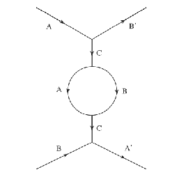
The corresponding amplitude for this diagram is [63]
| (2.1) |
where is the coupling constant, the two terms represent the two propagators and is the term associated with the loop, which is given by
| (2.2) |
with being the momentum of and the one of . A new term
| (2.3) |
is added at the amplitude for each new loop in the propagator. Considering a series of loops in the propagator , as shown in Fi. 2.3, the form of the propagator will be
| (2.4) |
with
| (2.5) |
where is called the irreducible self-energy.

2.3 Quantum chromodynamics
In this section we shall introduce basic common knowledge of Quantum Chromodynamics, in a way to be minimally self-contained.
Aside from the flavor, explained in Sec. 2.1, the quarks also posses another property called color charge. Quarks come in three primary colors: red (), green () and blue (). In the same way, antiquarks come in anticolors called antired (), antigreen (), and antiblue (). Each quark (or antiquark) can take only one of three values or charges.
Gluons, on the other hand, have their color charge constitued by a mixture of two colors (or anticolors). They can either be in a color singlet state
| (2.6) |
or in a color octet
| (2.7) |
where
| (2.8) |
But the strong force is of very short range, only eight kinds of gluons exist, excluding the singlet gluon of Eq. (2.6), because if a singlet gluon exists, it would be exchanged in a long-range interaction [64]. In the representation of the SU(3) group, explained in Appendix B, there are generators, so these eight color states are equivalent to the Gell-Mann matrices.
2.3.1 QCD Lagrangian
We begin writing down the QCD Lagrangian as [65]
| (2.9) |
where contains the light-flavor quark Dirac fields , the heavy-flavor quark Dirac fields and the pure-gluon part, with the lagrangians being
| (2.10) |
with , where is the gauge-covariant derivative
| (2.11) |
and is the gluon field strength tensor
| (2.12) |
where is the gluon field in the adjoint representation of SU(3) (explained in appendix B). The gluon field represents the gluon propagation in the strong interaction between quarks, being given by [66]
| (2.13) |
with each being a vector field and the index representing each of the eight possible combination of colors for the gluons .
The light and heavy quark mass matrices are
| (2.14) |
2.3.2 Chiral symmetry breaking
The mass scale is the value at which the theory becomes strongly coupled and nonperturbative and its value depends on the renormalization scheme used and on the number of active flavors (when the energy-momentum involved in the process allows to make active only a certain number of flavors, which means that heavier flavors will be suppressed even including the virtual state excitations). A common choice for the renormalization scheme is the Modified Minimal Subtraction scheme (). For the scheme, the values (in MeV) for different flavor numbers are
| (2.15) |
Since the masses of the light quarks , and are small compared with when just tree flavors are active (which is the case we consider), we may consider an approximation to QCD where the masses of these quarks are set to zero and do perturbation theory in about this limit. The limit is known as the chiral limit, where the light quark Lagrangian can be rewritten in terms of the operators and , (see appendix A for definitions on the gamma matrices) being given by [67]
| (2.16) |
and has a chiral symmetry under which the right and left-handed quark fields transform differently. Also, this Lagrangian is invariant under unitary transformations of the type
| (2.17) |
where and are independent SU(2) unitary transformation matrices satisfying .
The dynamical breaking of the symmetry can be written in terms of the nonzero value of the vacuum expectation value (v.e.v.) known as the quark condensate
| (2.18) |
where , and and are flavor indices. A nonzero value of the condensate implies a dynamically generated quark mass, since the dynamical mass is a function of the quark condensate [68].
Chapter 3 Heavy-Quarkonia production
This chapter aims to describe the production of heavy quarkonia by the models of photo-production featured in [49]. The process can be explained by various models, of which we focus here on the photon-gluon fusion (PGF) model and the pomeron exchange (PMEX) model, to be explained below. A separate section is dedicated to treat the specific case of production. This chapter also covers the estimate of heavy quarkonia production at an Electron-Ion Collider (EIC) and a brief mention of the possible production of heavy and heavy-light mesons at the Facility for Antiproton and Ion Research (FAIR).
3.1 Photo-production
The photo-production of heavy quarkonia is a process where a bound pair is produced by the interaction of a proton with a high energy photon . Since the proton is a complex system of valence quarks (the ones that contribute to a hadron’s quantum numbers), sea quarks (which are virtual quark-antiquark pairs () formed when a gluon of the hadron’s color field splits) and gluons, it is difficult to explicitly describe this process. Both models presented in this section are attempts to provide an explanation for this process.
3.1.1 Photo-gluon fusion model
In the photon-gluon fusion (PGF) model the photon fuses with a gluon emitted from the proton and split into a pair, as shown in Fig. 3.1. The model depends on the photon-gluon cross section, which is similar to (QCD analogue of) the pair production in photon-photon collisions, being given by [69]
| (3.1) |
where is the electromagnetic fine structure constant, and are are the electric charge and the mass of the heavy quark respectively, is the strong coupling at ( at ), , where is the proton mass and is the photon energy, and is defined as .
The cross section of heavy quarkonia photo-production is then given by
| (3.2) |
with being the gluon distribution of the proton at the mass scale , and is an adjustable parameter that accounts for the fraction of the specific quarkonium bound states available in the mass region between and , and and are the intermediate state hadrons for and , respectively.

3.1.2 Pomeron-exchange model
The phenomenological pomeron exchange (PMEX) model is used to study the photo-production of vector mesons (V), which is a process of the type , represented by the Feynman diagram shown in Fig. 3.2. A pomeron (PM) is a particle of a pre-QCD approach to describe hadron interactions, known as Regge theory (see Appendix C). In this theory, the pomerons (see Appendix D) are the objects exchanged by the interacting hadrons.
Bringing this description to a QCD view, one can interpret a two-gluon exchange (or even several gluon ladders) as if the gluons are “reggeised”, meaning that it can be taken as a pomeron exchange [70].
The is parameterized as a function of the photon-proton () center-of-mass energy [71], and for the and cases we have
| (3.3) |
where contains only the parameter for the photon-pomeron center of mass (no meson exchange is considered), and the free parameter is experimentally determined.

3.2 Electro-production
Now we discuss the electro-production of vector mesons, with the process represented in Fig. 3.3 for both the PGF and PMEX models. We express the cross section of as
| (3.4) |
where is the cross section for the vector meson production by a virtual photon, is the final state invariant mass [72] and
| (3.5) |
which is the probability of electron emitting virtual photons with energy and , where is the four-momentum of the intermediate photon, and minimum [73].
Since the vector meson production by the virtual photon is -dependent, the models described above may be used to calculate the electro-production cross-sections of heavy quarkonia.


3.3 Production
This section covers the methods presented in [74] to obtain the cross section of the inclusive () production , represented in Fig. 3.4. Considering now the production of a pseudo-scalar meson, it can be described as a production of heavy quark-antiquark pair .
For a general Fock state (see Appendix E), where we consider the state of the pair in the various Fock-state components (e.g. , which includes a dynamical gluon), the pair can be in either a color-singlet state or a color-octet state, and its angular-momentum state denoted by , where is the total spin of the quark and antiquark, (or ) is the orbital angular momentum, and is the total angular momentum. In the Fock state , the pair must be in a color-singlet state and in an angular momentum state , because the color-octet state evolves non-perturbatively into a physical color-singlet state by emission of one or more gluons [75].
Using a nonrelativistic QCD (NRQCD) approach, one needs to take into account the contributions of the color singlet (CS) and color octet (CO) components, with unknown nonperturbative long-distance matrix elements (LDME), that are treated as free parameters. LDMEs are organized into a hierarchy according to their scaling with , the typical velocity of the heavy quark. The calculation of the cross section involves colored heavy quark-antiquark pairs in and configurations, represented by the sates, where the indexes (1,8) represent whether the components are color siglet or color octet.
The cross section for production of a quarkonium state can be factorised as
| (3.6) |
where the s are short-distance coefficients, are operators of dimension describing the long-distance effects and is the heavy quark mass.
To study the production cross section, we write the Fock space expansion (See Appendix E) for the physical [76], with the main contributions to the cross section being the terms [75]
| (3.7) |
The color-octet state () becomes a physical by emitting a gluon (), then the case considered is
| (3.8) |
so the differential cross section for the production with specific angular momentum and colour states is given by [74]
| (3.9) | |||||
where is the transverse momentum of the final quarkonium, is the value of the heavy quarkonum wave function in the CS state at the origin, and the following notations for CO LDME are used [77]
| (3.10) | |||||
| (3.11) |

3.4 Production at EIC
In nuclear physics, many questions arise from the current fundamental understanding of QCD. How quarks and gluons inside the proton combine their spins to generate the proton’s overall spin (1/2), and how these objects are distributed in space and momentum inside the nucleon? Why quarks or gluons must remain confined? There is a boundary between the saturated gluon density and the more dilute quark-gluon matter regions? And if so, how does the quark-gluon distribution changes from each other?
To provide answers to these questions, electron-ion colliders (EIC) is being constructed. In addition, the electro-production of heavy quarkonia are among the key reactions that are going to be measured on electron-ion colliders. In the USA, two independent designs for a EIC are being considered using already existing infrastructure and facilities. At the Jefferson Laboratory (JLab) a new electron and ion collider ring complex will be added together with the already existing 12GeV upgraded Continuous Electron Beam Accelerator Facility (CEBAF), which in a recent experiment [2], a photon beam was used to produce a meson near-threshold, which was identified by its decay into an electron-positron pair. While at Brookhaven National Laboratory (BNL), the eRHIC design utilizes a new electron beam facility based on an Energy Recovery Linear Particle Accelerator (ERL) to be built inside the (Relativistic Heavy Ion Collider) RHIC tunnel to collide with RHICs existing high-energy polarized proton and nuclear beams. The schematics of both colliders are shown in Fig. 3.5. More information on this can be found in [78].

3.5 Production at FAIR
The Facility for Antiproton and Ion Research (FAIR) is currently under construction as an international facility at the campus of the GSI Helmholtzzentrum for Heavy-Ion Research in Darmstadt, Germany. It will be an accelerator-based research facility in many basic sciences and their applications. FAIR will cover researches on the structure and evolution of matter on both the microscopic and the cosmic scale. It will be able to explore hadron structure and dynamics exploiting proton-antiproton annihilation. With the construction of the FAIR facility, heavy and heavy-light mesons will be produced copiously by the annihilation of antiprotons on nuclei [3]. The facility layout is shown in Fig. 3.6.

Chapter 4 Quark-meson coupling model
The quark-meson coupling (QMC) model is a quark-based model for nuclear matter and finite nuclei by describing the internal structure of the nucleon using the MIT bag (original version), and the binding of nucleons by the self-consistent couplings of the confined light quarks to the scalar-, isoscalar-vector- and isovector-vector- meson fields generated by the confined light quarks in the nucleons [41, 58, 60]. In a nuclear medium, the hadrons with light quarks are expected to change their properties, and thus affect the interaction with nucleons, what makes the QMC model a useful model to describe the changes of the internal structure of hadrons in a nuclear medium.
Although the QMC model was invented by Guichon [41], a similar model for nuclear matter was studied around the same time by Frederico et al. [79], where the nucleon on nuclear matter properties is investigated within a -- model, and the quark confinement explained by a quark potential which takes the form of a harmonic oscillator. Also, in the early 90’s, Banerjee [80] studied the changes in the structure of a nucleon when it is placed in nuclear matter, Naar and Birse [81] studied nucleon properties in nuclear matter by treating it within a color-dielectric model, and Mishra et al. [82] investigated nuclear matter in the relativistic Hartree approximation using a - model.
In this chapter, the basis of this model will be set by describing the MIT bag model and its mathematical structure. Based on that, the description of the QMC model will be followed by details on the calculation of the in-medium masses of the and mesons, with the latter being obtained for the first time in symmetric nuclear matter.
4.1 MIT bag model
Initially, a kind of bag model was proposed by P.N. Bogoliubov in 1967 [83] to model the atomic nucleus as a system of independent quarks in a confining potential. The Bogoliubov model considered three massless quarks in a vacuum cavity of radius chosen so as to relate the energy of the 3 quarks to the mass of the hadron. This cavity contained a finite, spherical, square well potential, which finally was set to infinity.
This model was then improved seven years later by a group of five scientists from the Massachussets Institute of Technology (MIT) [84, 85], that stated that strongly interacting quarks are in a finite region of space to which fields are confined. This region is called a bag (hence the name MIT bag model). It also provided a natural explanation for the confinement phenomenon, which is accomplished within the model by surrounding the finite region with a constant (potential) energy per unit volume, .
Now we describe the mathematics of the MIT bag, emphasizing some of its aspects that will be of use further ahead on the study of the QMC model, that is, to include the influence of external fields to the bag.
We start by considering a system of three quarks, each with mass , in a scalar potential , where these quarks are confined in a cavity (in reality by the strong interactions among quarks mediated by the (exchanged) gluon fields) and under external fields. The enclosed region in which the quarks can move has an radius , and is subjected to a pressure . The bag radius is determined by the stability equation , where is the bag energy. This system is represented here in Fig. 4.1.
The quarks inside the cavity may interact with external fields of scalar- and vector-, types. This means that , and meson exchanges may occur.
The Dirac equation which describes this system has the form
| (4.1) |
with . So the Dirac equation containing real fields is
| (4.2) |
where is the isospin third component and , and describe the interactions between quarks and the fields , and through the quark-meson coupling constants , and .

4.2 Quark-meson coupling model
The quark-meson coupling model is a quark-based model that describes nuclear matter by nucleons and mesons, where the quark structure of the nucleon is modified by the surrounding nucleons and meson fields [41]. The infinite nuclear matter at normal density (or at a not very higher density, up to about 3 times the nuclear matter saturation density, since at higher densities the model description with nonoverlapping MIT bags for the nuclear medium may not be proper, and also quark-hadron mixed phase is expected to appear.) is a uniform distribution of nucleons interacting through the exchange of mesons which are coupled directly to the quarks, and only the -exchange, the (time component of the) -exchange () and the -exchange (, in the isospin asymmetric nuclear matter, where is determined by the difference in proton and neutron densities, ) contributes to the isospin asymmetric nuclear matter.
4.2.1 QMC description of nuclear matter
We start the description of the internal structure of the nucleon by treating it classically (at first). The descriptions of this subsection, subsections 4.2.2 and 4.2.5 are from [58]. It is then useful to take the coordinates in the rest frame of the nucleus (NRF), denoted by . In this frame the nucleon follows a classical trajectory, , and the instantaneous velocity of the nucleon is given by . We then define an instantaneous rest frame for a nucleon at each time (IRF), which is denoted with primes , and are related to the NRF coordinates by the Lorentz transformation (with = 1):
| (4.3) |
where and are, respectively, the parallel and transverse components to the velocity and is the rapidity defined by .
We can thus describe the internal structure of the nucleon in the IRF, adopting the the static spherical cavity approximation to the MIT bag. The appropriate Lagrangian density in the IRF is then [58, 62]
| (4.4) |
with being the bag constant, the bag volume, the bag radius for the nucleon and the position of the quark from the center of the bag in the IRF, where the 4-vector is denoted as .
Now to include the effects of the interactions with the surrounding nucleons, we incorporate the and fields generated by them. In the NRF they are functions of position, so we express them in the IRF by Lorentz transformation
| (4.5) |
where the subscript stands for the IRF. Now we can write the interaction as
| (4.6) |
with the coupling constants and . We do not include, however, the effect of the meson field (at least for now).
To construct the hamiltonian in the IRF, we shall evaluate the interaction term at equal time for all in the bag. Supposing that at time the bag center is located at in the IRF, in the NRF it will be located at at time , defined by
| (4.7) |
We then express the and fields as
| (4.8) |
where .
Thus, in the IRF the interaction Lagrangian is
| (4.9) |
and the corresponding Hamiltonian expressed in two pieces :
| (4.10) |
where is treated as a perturbation.
We then write a complete orthogonal set of eigenfunctions for the quark field, denoted by , where is a collective symbol to label the quantum numbers
| (4.11) |
with being a parameter. The lowest positive eigenfunction is given by
| (4.12) |
with , being the (Pauli 2-component spinor) spin function and
| (4.13) |
where is the eigenvalue for the lowest mode, which satisfies the boundary condition at the bag surface, , where and are the speherical Bessel functions.
The quark field is then expanded as
| (4.14) |
with being the annihilation operator for the quark and .
Considering now just the free Hamiltonian, we choose the effective quark mass as , and so we find the leading part of the energy and momentum operators in the IRF to be [58, 62]
| (4.15) |
where the frequency depends on because the effective quark mass varies, depending on position through the field. The nucleon is supposed to be described in terms of the three quarks in the lowest mode (), and since it should remain in that configuration as changes, the gradient term in the momentum operator becomes zero because of parity conservation. Then, the energy and momentum in the IRF can be written as
| (4.16) |
with the effective nucleon mass
| (4.17) |
with the bag radius given by the stability equation
| (4.18) |
Now we use the Lorentz transformation to express these terms in the NRF as
| (4.19) |
So the leading term in the energy can be written
| (4.20) |
with the effective nucleon mass in matter taking the form
| (4.21) |
where we parameterize the sum of the center of mass (c.m.) correction and gluon fluctuation corrections to the bag energy by , with these fluctuations and change in the center of mass arising due to the movement of the valence quarks and gluons inside the nucleon bag, where is assumed to be independent of the nuclear density, with the parameters and fixed by the free nucleon mass ( = 939 MeV) [62].
This is justified by the Born-Oppenheimer approximation, according to which the internal structure of the nucleon has enough time to adjust the varying external field so as to stay in its ground state.
Now we estimate the perturbation term by expanding and in powers of
| (4.22) |
and computing the effect to first order. To this order several terms give zero because of parity and one is left with
| (4.23) |
where is setted, with the spin projection of the quark in the lowest mode . Then
| (4.24) | |||||
with
| (4.25) |
where and are the upper and lower components of the quark wave function, respectively. And using the wave function of the MIT bag
| (4.26) |
The integral depends on through the implicit dependence of and on the local scalar field. Its value in the free case, , may then be expressed in terms of the nucleon isoscalar magnetic moment: with and = 2.79 and = -1.91 the experimental values (all in units of ). Using this, may be written by
| (4.27) |
with and being respectively the nucleon spin and angular momentum operators.
The interaction of the magnetic moment of the nucleon with the magnetic field of the meson seen from the rest frame of the nucleon induces a rotation of the spin as a function of time. But even when is zero, the spin even so would rotate because of the Thomas precession, which is independent of the structure and other effects [86]
| (4.28) |
where
| (4.29) |
The total spin-orbit interaction comes from combining this precession with the effect of
| (4.30) |
where
| (4.31) |
and
| (4.32) |
For completeness, we shall introduce the effect of the meson field. We do this by adding the following interaction term to
| (4.33) |
where is the -meson field with isospin component in the IRF, and are the Pauli matrices acting on the quark fields. In the mean field approximation only contributes (the mean field is of a isovector type, so it must be in the third direction of isospin (proportional to )). If the mean field value of the time component of the field is denoted by in the NRF, the results can be transposed for the field. The difference coming from the trivial isospin form factors
| (4.34) |
where is the nucleon isospin operator.
In the NRF, the energy and momentum of the nucleon moving in the meson fields are
| (4.35) |
with
| (4.36) | |||||
and
| (4.37) |
To finally quantize the model, the following Lagrangian is found by realizing that the above energy-momentum expressions can be derived from it
| (4.38) |
Then, the non-relativistic expression of the Lagrangian may be
| (4.39) |
which leads to the Hamiltonian
| (4.40) |
where the spin-orbit interaction is reintroduced in the potential . Thus, the nuclear, quantum Hamiltonian for the nucleus with atomic number is given by
| (4.41) |
Now we present the equations for the meson fields. For the meson-field operators , the equations of motion are given by
| (4.42) |
where the masses of , and mesons are , and , respectively.
To apply the mean field approximation to these meson fields, the mean fields are calculated as the expectation values with respect to the nuclear ground state :
| (4.43) |
then we need the expectation values of the sources
| (4.44) |
In the mean field approximation the sources are the sums of the sources created by each nucleon. We shall not treat now the source for the meson for simplicity. Thus we write
| (4.45) |
where is the matrix element in the nucleon located at at time . In the Born-Oppenheimer approximation, which is used in this model, the nucleon structure is described by 3 quarks in the lowest mode. In the IRF
| (4.46) |
In the NRF, the sources are given by
| (4.47) |
These sources can be rewritten in the form
| (4.48) |
with the sources in momentum space being
| (4.49) |
The mean field expressions for the meson sources are then given by
| (4.50) |
where the last equation follows from the fact that the velocity vector averages to zero (see Eq. (4.2.1)). This can be simplified even further to [58]
| (4.51) |
with the scalar (), baryon () and isospin () densities of the nucleon in the nucleus
| (4.52) |
where the () in the first equation, for the -th nucleon at is given by
| (4.53) |
in the MIT bag model. Then, combining the Eqs. (4.2.1), (4.2.1) and (4.2.1), we finally get the equations for , and
| (4.54) |
where () and the meson-nucleon coupling constants are defined by
| (4.55) |
The energy carried by the mean fields is
| (4.56) |
In order to make the calculation for finite nuclei self-consistent, the following steps must be taken:
- 1.
When using the MIT bag as the quark model for the nucleon, choose a quark mass and fix the bag parameters and to fit the nucleon mass and bag radius.
- 2.
Assume that the coupling constants and the masses of the mesons are known.
- 3.
- 4.
Guess initial forms of the densities , and in Eqs. (4.2.1).
- 5.
Fixed , and , solve Eqs. (4.2.1) for the meson fields.
- 6.
- 7.
Solve the eigenvalue problem given by the nuclear Hamiltonian (Eq. (4.41)) and compute , and .
- 8.
Go to step 5 and iterate until self-consistency is achieved.
4.2.2 Relativistic model
Now we express the model in the framework of relativisitic field theory at the mean field level. The Lagrangian density for the symmetric nuclear system may be written as [62]
| (4.57) |
where , and are the nucleon, and operators, respectively, and the free meson Lagrangian in the last term is given by
| (4.58) |
The nucleon mass can be separated as
| (4.59) |
and so the Lagrangian density can be rewritten as
| (4.60) |
In the mean field approximation, we can replace the meson-field operators by their expectation values in the Lagrangian as and . Then, the nucleon and meson fields satisfy the equations:
| (4.61) |
where
| (4.62) |
To include now the -meson contribution, and also to the Coulomb interaction, the following interaction Lagrangian must be added to Eq. (4.60) [62]
| (4.63) |
The expressions for the and Coulomb fields can be achieved by including trivial isospin factors or . The effective Lagrangian density for the QMC model in the mean field approximation is given by
| (4.64) | |||||
4.2.3 Nuclear matter properties
Considering the rest frame of infinitely large, symmetric nuclear matter, we set to zero the Coulomb field in Eq. (4.64) Lagrangian, and drop all the terms with any derivatives of the fields, and so it is done in the equations of motion in Eq. (4.2.2). So in the nuclear matter limit, within the Hartree mean-field approximation, the baryon and scalar densities with the nucleon Fermi momentum are respectively given by [62, 87, 88]
| (4.65) |
where is the (constant) value of the effective nucleon mass at a given density, shown in Fig. 4.2 [89]. The meson mean fields and are given by Eq. (4.2.2) with the derivatives of the fields set to zero
| (4.66) |
where is the constant value of the scalar density ratio (see Eq. 4.55).

The total energy per nucleon can be evaluated after one solves the self-consistency for the field
| (4.67) |
The coupling constants and are determined so as to fit the binding energy (-15.7 MeV) per nucleon at the saturation density, = 0.15 fm-3, for symmetric nuclear matter. The coupling constants at the nucleon level are = 5.39 and = 5.30. We show in Fig. 4.3 the calculated values of the total energy per nucleon, obtained using the determined quark-meson coupling constants [61].

The effective light-quark mass in nuclear medium is given by , with being the interaction of the light-quark with the scalar field. The effective light-quark mass, together with the corresponding mean field potentials felt by the light-quarks, and , are shown in Fig. 4.4 [61]. One should have in mind that the negative value of only reflects the strength of the attractive scalar potential, and thus the interpretation that the mass for a physical particle is positive should not be applied here.

4.2.4 Hadron properties in nuclear matter
The original version of the QMC model is based on the MIT bag, and so, the Dirac equations for the quarks and antiquarks in nuclear matter, in bags of hadrons , ( or , and or ) neglecting the Coulomb force are given by ( bag radius)
| (4.68) | |||
| (4.69) | |||
| (4.70) |
The (constant) mean-field potentials for the light and quarks in nuclear matter are defined by , , , with the , and being the corresponding quark-meson coupling constants, as before.
The static solution for the ground state quarks (antiquarks) with flavor in the hadron is written as , with normalization factor and as the corresponding spin and spatial part of the wave function. The eigenenergies for the quarks and antiquarks in in units of are [59]
| (4.71) | |||
| (4.72) | |||
| (4.73) |
The light quark field is modified by the term which acts as . Then, the mass modification is expected to occur to the hadrons containing those light quarks inside their bags. The mass of a hadron in a nuclear medium is calculated by
| (4.74) | |||
| (4.75) |
with , where and , with being the lowest mode bag eigenfrequencies. is the bag constant, and () are the lowest mode quark (antiquark) numbers for the quark flavors and in the hadron , and the parameterize the sum of the center-of-mass and gluon fluctuation effects and are assumed to be independent of density [58]. Since and are modified in medium when contains light quarks, is also modified in medium.
The bag radius of the nucleon in free space input value chosen is = 0.8 fm. The parameter is determined by the nucleon mass 939 MeV with 0.8 fm, and is fixed to reproduce the hadron mass, while the quark-meson coupling constants, , and were determined by the fit to the saturation energy (-15.7 MeV) at the saturation density ( fm-3) of symmetric nuclear matter for and , and the bulk symmetry energy (35 MeV) for [41, 62] (see Eq. 4.55).
4.2.5 QMC description of finite nuclei
The description of a finite nucleus with different numbers of protons and neutrons () needs to include the contributions of the meson, as well the Coulomb force. The following equations for static, spherically symmetric nuclei, comes from the variation of [62]
| (4.76) | |||||
| (4.77) | |||||
| (4.78) | |||||
| (4.79) | |||||
where and
| (4.80) | |||||
| (4.81) | |||||
with labeling the quantum numbers, being the energy, and and being, respectively, the radial part of the upper and the lower components of the solution to the Dirac equation for the nucleon [90, 91]
| (4.82) |
under the normalization condition
| (4.83) |
where is a two-component spinor and is the angular part wave functions.
The angular quantum numbers are specified by and the eigenvalue of the isospin operator by . Also, it is well parametrized the -dependent coupling as,
| (4.84) |
where is a slope parameter for the nucleon, ranging = 8.97 9.01 10-4 (MeV-1), depending on the parameterization for the mass in matter. The total energy of the system is then given by
| (4.85) | |||||
4.3 and meson in-medium masses
In this section we focus on the properties of and mesons in nuclear matter, calculating their effective masses using the QMC model. This is enough, since the vector potentials appearing in the and loops in the self-energy calculation, or in the energy-contour integral for each loop, cancel out, and this is consistent with the baryon number conservation at the quark level.
To determine the in-medium masses of the and mesons by the Eq. (4.74) (, and ), we obtain the following bag parameters for the bag radius of the nucleon in free space with value = 0.8 fm as input: = 5.69, = 2.72, = 9.33, = 170 MeV, = -1.136 and = -1.334, with he vacuum mass values (input) = 5279 MeV and = 5325 MeV, and the chosen values (, ) = (5, 4200) MeV for the current quark masses. The QMC model predicts a similar amount in the decrease of the in-medium effective Lorentz-scalar masses of the and mesons in symmetric nuclear matter as shown in Fig. 4.5. At the mass shifts of the and mesons are respectively, MeV and MeV, the difference in their mass shift values appears in the next digit. To calculate the and meson self-energies in symmetric nuclear matter by the excited and meson intermediate states in the loops, we use the calculated in-medium masses of them shown in Fig. 4.5.

Chapter 5 mass shift and bound state energies
The mass of the in-medium meson (and of heavy quarkonia in general) is also expected to be modified as a result of the interaction between with nuclei. But differently from the and mesons considered before in the last chapter, heavy quarkonium has no light quarks, and so, interactions involving light-quark or light-flavored hadron exchanges do not occur in the lowest order. However, the heavy quarkonium intermediate state hadrons do contain light quarks, what makes the excitation of these intermediate state hadrons a possible mechanism for the heavy quarkonium interaction with the nuclear medium. The mass shift in nuclear medium is then studied as the contribution of its possible intermediate state mesons to its self-energy by employing effective Lagrangians for the coupling of these mesons to [92]. The resultant negative shift in the mass is interpreted as an attractive potential that can bind the meson to nuclei.
In this chapter, the mass shift in nuclear medium is studied using effective Lagrangians, which are obtained from a unified SU(5) symmetry Lagrangian by minimal substitutions, introducing also an extra (anomalous coupling) Lagrangian for the -loop case. We present here the results for the contributions of the , and the meson loops to the self-energy, where the in-medium masses of the and mesons are obtained based on the QMC model, as explained in Chapter 4. This chapter also includes a comparison between the total ( + + ) meson loop contribution and its correspondent ( + + ) in the case. The -nucleus potential is calculated for various nuclei (4He, 12C, 16O, 40Ca, 48Ca, 90Zr and 208Pb) using a local density approximation, and the bound state energies are obtained by numerically solving the Klein-Gordon equation (originally the Proca equation) for each nucleus.
5.1 Effective Lagrangians
The mass shift in medium comes from the modification of , and meson loop contributions to the self-energy relative to that in free space, which is calculated, based on a flavor SU(5) symmetry using an effective Lagrangian density [93] (hereafter we simply call Lagrangian). The free Lagrangian for pseudoscalar and vector mesons is given by
| (5.1) |
with
where and (suppressing the Lorentz indices for ) are, respectively, the pseudoscalar and vector meson matrices in SU(5):
The following minimal substitution is introduced to obtain the couplings (interactions) between pseudoscalar mesons and vector mesons, in a similar way as the substitution to get the interaction of a charged particle with a electromagnetic field is introduced [65]:
| (5.2) | |||
| (5.3) |
Then, the effective Lagrangian is obtained as,
| (5.4) | |||||
Expanding this in terms of the and matrices above, we obtain the following interaction Lagrangians [93]
| (5.5) | |||||
| (5.6) | |||||
where the following convention was adopted
In addition we also include the anomalous-coupling [94, 95] interaction Lagrangian, similar to the case of that was introduced in the interaction Lagrangian in Refs. [96, 9],
| (5.7) |
where, we assume , the corresponding relation adopted for the case [9].
5.2 Coupling constants
The values of the coupling constants appearing in the Lagrangians of the last section are here determined by the Vector Meson Dominance model (VMD) [93]. In this model, represented in Fig. 5.1, the virtual photon in the process is coupled to the vector mesons , and . If we consider the case of zero momentum transfer, we can use the following relation:
| (5.8) |
where photon-vector-meson mixing amplitude is determined from the vector-meson decay width
| (5.9) |
with being the fine structure constant, which is a dimensionless measure of the strengths of the electromagnetic interactions. We have then
| (5.10) |
thus obtaining
| (5.11) |

5.3 Self-energy
The in-medium potential for the meson is given by the difference between the in-medium, , and free space, , masses of ,
| (5.12) |
with the free space physical mass being reproduced first by,
| (5.13) |
where is the bare mass, and the total self-energy is calculated by the sum of the contributions from the free space , and meson loops in the case we include all the meson loops considered in this study. Note that, we ignore the possible width, or the imaginary part in the self-energy in the present study. The in-medium mass, , is calculated likewise, by the total self-energy in medium using the medium-modified and meson masses with the same value fixed in free space. We remind that the value depends on the loops included in the self-energy of the in free space.
The S-Matrix is (see Appendix F)
| (5.14) |
where the second term containing the time order operator contains the information on the interactions and is the invariant amplitude, which is the probability amplitude of transition from the incoming states to the outgoing states in a scattering process. We then find the self-energy contribution for each interaction lagrangian in equations (5.5), (5.6) and (5.7) by making use of the following relation (see expression (2.1))
| (5.15) |
We then sum each meson loop contribution for the self-energy as
| (5.16) |
where and is the product of vertex form factors (to be discussed later). The for each meson loop contribution is given, similarly to the case [9],
| (5.17) | |||
| (5.18) | |||
| (5.19) |
where , , and
| (5.20) |
with
| (5.21) | |||||
| (5.22) | |||||
| (5.23) | |||||
| (5.24) |
where , and the is taken at rest, .
We use phenomenological form factors to regularize the self-energy loop integrals following Refs. [9, 97],
| (5.25) |
For the vertices , and , we use the form factors , , and , respectively, with () being the corresponding cutoff mass associated with () meson, and the common value, , will be used in this study.
We have to point out that the choice of the cutoff mass values in the form factors for the , and vertices has nonnegligible impact on the results. But the form factors are necessary to include the effects of the finite sizes of the mesons for the overlapping regions associated with the vertices. The cutoff values may be associated with the energies used to probe the internal structure of the mesons or the overlapping regions associated with the vertices. When these values get closer to the corresponding meson masses, the Compton wavelengths () associated with the values of are comparable to the sizes of the mesons (for and , we have ), and the use of the form factors does not make reasonable sense. Then, in order to have a physical meaning, we may be able to constrain the choice for the cutoff mass values, in such a way that the form factors reflect the finite size effect of the participating mesons reasonably. Later, an analysis on this issue will be made taking the , and vertices as examples.
By the heavy quark and heavy meson symmetry in QCD, the charm and bottom quark sectors are expected to have mostly similar properties (but quantitatively need to be shown if possible). We thus follow this naive expectation and choose the similar cutoff mass values as the ones used in the previous work of the mass shift [7], varying the values between , but with the larger upper values, since the and masses are larger than those of the and mesons.
5.4 Mass shift
5.4.1 Results for mass shift
In the following we present the results for the in-medium mass shift of meson together with each meson loop contribution for five different values of the cutoff mass , where we use the in-medium and meson masses shown in Fig. 4.5. The values used for the free space masses of , and mesons are, respectively, 9460, 5279 and 5325 MeV [98].
The values of , as well as each loop contributions to , in the range of the cutoff masses are: 9653 to 9802 MeV for the total loop contribution, 9836 to 10123 MeV for the ( + ) total loop contributions and 19649 to 24966 MeV for the ( + + ) total loop contributions. The loop contribution to ranges from 193 to 342 MeV, the contribution corresponding to the loop being 186 to 332 MeV, and the one from the loop ranging from 10003 to 15244 MeV.


In Fig. 5.2 we show the mass shift, taking the total contribution to be the meson loop for five values of the cutoff mass , 2000, 3000, 4000, 5000 and 6000 MeV (these values will be applied for all the studies in the following with ). As one can see, the effect of the decrease in the meson in-medium mass yields a negative mass shift of the . The decrease of the meson mass in (symmetric) nuclear matter enhances the meson loop contribution, thus the self-energy contribution in the medium becomes larger than that in the free space. This negative shift of the mass is also dependent on the value of the cutoff mass , i.e., the amount of the mass shift increases as value increases, ranging from -16 to -22 MeV at the symmetric nuclear matter saturation density, fm-3.
Next, in Fig. 5.3 we show the mass shift taking the total self-energy contribution to be the meson loops. The contributions are shown for the meson loop (top left), meson loop (top right), and the total meson loops (bottom). The total mass shift at ranges from -26 to -35 MeV for the same range of the values.
Finally, we show in Fig. 5.4 the mass shift taking the total self-energy contribution to be the meson loops. The contributions are shown for the meson loop (top left), the meson loop (top right), meson loop (bottom left), and the total meson loops (bottom right). The total mass shift at ranges from -74 to -84 MeV for the same range of the values.
It is important to note that due to the unexpectedly larger contribution from the heavier meson-pair meson loop ( meson loop) to the mass shift than the other lighter-meson-pair loops and presented in Fig. 5.4, we regard the form factor used for the vertices in the meson loop may not be appropriate, and need to consider either different form factors, or adopt an alternative regularization method in the future.
Summary for the mass shift:
The mass shift is shown separately in Figs. 5.2, 5.3
and 5.4, by the difference in the intermediate states contributing for
the total self-energy, namely, by the ,
, and meson
loops. The corresponding mass shift at ranges,
(-16 to -22) MeV, (-26 to -35) MeV, and (-74 to -84) MeV, for the adopted range
of the ) values.
The results indicate that the dependence on the values of the cutoff
mass is rather small compared to that of the for the case as will be discussed later,
and this gives smaller ambiguities for our prediction
originating from the cutoff mass values.
5.4.2 Comparison with mass shift


The issue of the larger contribution from the heavier vector meson loop, in the present case meson loop, was already observed in a previous study of the mass shift due to the heavier meson loop contribution, where a similar nongauged effective Lagrangian was used and no cutoff readjustment was made for the heavier vector meson intermediate states [9]. The cutoff mass value readjustment in a proper manner is important, because it controls the fluctuations from the shorter distances. However, we do not try this in the present exploratory study, since we first need to see the bare result without readjusting, so that we are able to compare with those of the case, focusing on the heavy quark and heavy meson symmetry.
We have calculated the total () meson loop contribution for the mass shift as featured in Ref. [7] using the same effective Lagrangian and cutoff mass values to compare with the total () meson loop contribution in the mass shift. The free space masses of the , and mesons used are 3097, 1867 and 2009 MeV [98], respectively.
The values of , as well as each loop contributions to , in the range of the cutoff masses are: 3120 to 3316 MeV for the total loop contribution, 3138 to 3499 MeV for the ( + ) total loop contributions and 4462 to 12000 MeV for the ( + + ) total loop contributions. The loop contribution to ranges from 23 to 219 MeV, the contribution corresponding to the loop being 18 to 196 MeV, and the the one from the loop ranging from 1336 to 8792 MeV.
The result is presented in Fig. 5.5. The meson loop contribution for the mass shift ranges from -61 to -164 MeV at , which is mostly larger than that of the (-67 to -77 MeV at ) for the same range of the cutoff mass values in the corresponding form factors. Note that, the larger cutoff mass values, and MeV, may not be appropriate as will be discussed in the following. We can see from Fig. 5.5 that the closer the cutoff mass value gets to the mass, less pronounced the negative mass shift becomes, until it reaches a transition point (when is larger than the free space mass), where the potential starts to become even positive. Naively, according to the second order perturbation theory in quantum mechanics, they should give the negative contribution, but the positive contributions for and MeV, thus suggest that such larger values of the cutoff mass may not be justified for the form factor used. One can expect a similar behavior in the meson loop in the total meson loop contribution when the cutoff mass value gets closer to the mass. Indeed, such behavior is observed for the and meson loop contributions, for the cutoff mass values larger than 10000 MeV. As already commented in Sec. 5.3, the large cutoff-mass values than the corresponding vector meson mass means that the distance for the interaction between the vector meson and the intermediate state meson included is shorter than the meson overlapping region, and a physical picture as an isolated vector meson is lost — one also needs to consider the quark-quark, quark-antiquark, and antiquark-antiquark interactions and/or the corresponding correlations at the quark level in such short distances, where the present approach does not have.
The bad high-energy behavior of the vector meson propagator is well known. To evaluate amplitudes in high-energy region that contain vector meson propagators in spontaneously broken gauge theory such as the weak interaction in the Standard Model, the generalized renormalizable gauge ( gauge) is usually used. This gauge uses an adjustable parameter to include other existing gauges as special cases, such as the , and ’t Hooft-Feynman gauges. In the gauge, the massive-vector-boson propagator is
| (5.26) | |||||
where is the vector-boson mass and can vary continuously from 0 to .
The gauge is connected to the other gauges as follows:
- 1.
gauge: Is a generalization of the Landau gauge in QED, obtained from the gauge by setting = 0.
- 2.
’t Hooft-Feynman gauge: Is obtained for = 1. In this gauge, the vector-boson propagator is proportional to the metric (see appendix A for the metric convention), and the unphysical scalar-boson propagator has a pole at .
- 3.
gauge: There’s no unphysical scalar bosons in this formulation, so the vector-boson propagator is just
(5.27) which is equivalent as taking in the gauge.
The gauge with (’t Hooft-Feynman gauge) makes the high-energy behavior of the vector meson propagators similar to that of the spin-0 meson propagators [99, 100, 101, 102]. gauge then removes unphysical degrees of freedom associated with the Goldstone bosons. In the present case, we cannot justify to use such vector meson propagators, so we need to tame the bad high-energy behavior phenomenologically. We can do this by introducing a phenomenological form factor for the meson loop case. But for the and meson loops we simply discard their contributions in the present study as was practiced in Ref. [7]. Therefore, our prediction should be regarded based on the minimum contribution with respect to the intermediate state meson loops, namely by only the meson loop contribution as in Ref. [7], which took only the meson loop contribution for estimating the mass shift. Regarding the form factors, another choice of form factors is possible to moderate the high-energy behavior [50, 103, 104], and an initial study of using a different form factor will be performed in Sec. 7.2.
Furthermore, although we have chosen the same coupling constants for , , and , it is certainly possible to use the different values for the coupling constants. Some studies of SU(4) flavor symmetry breaking couplings in charm sector offer alternative ways for the calculation of these coupling constants. This can be extended to include SU(5) symmetry breaking couplings. But for the flavor SU(5) sector, the breaking effect is expected to be even larger than that for the SU(4) sector, since bottom quark mass is much heavier than the charm quark, and the SU(5) symmetry breaking is expected to be larger. There are some studies focused on the SU(4) symmetry breaking of the coupling constants, although the results are not conclusive. A recent calculation [105] used dispersion formulation of the relativistic constituent quark model, where the couplings were obtained as residues at the poles of suitable form factors. Two other studies are made by the Schwinger-Dyson-equation-based approaches for QCD [106, 107, 108]. In the both approaches, the obtained results for the SU(4) symmetry breaking are considerably larger than those obtained using QCD sum-rule approach. We plan to do more dedicated studies on the issues in the future. In the present study, the coupling constant contains SU(5) symmetry breaking effect with respect to that of the corresponding charm sector, , where both of them are determined using the VMD model with experimental data.
We emphasize again that, the prediction for the mass shift made solely by the meson loop, gives -3.0 to -6.5 MeV based on Refs. [9, 7] (-5 to -21 MeV for the same range of the cutoff value, 2000 to 6000 MeV), while for the mass shift, taking only the contribution from the meson loop, gives -16 to -22 MeV. In Sec. 7.1 we will make some study for the and mass shifts focusing on the SU(5) symmetric coupling constant between the charm and bottom sectors, as well as a coupling constant in a broken SU(5) symmetry scheme between the and .
One might question further, as to why the () mass shift is larger than that of the (), although we have already commented the main reason by the larger coupling constant obtained by the VMD model with the experimental data. (The other way, why the bottom sector coupling constant is larger than that of the charm sector, or the corresponding experimental data in free space to determine the coupling constant is larger.) Of course, the heavier and meson masses than the corresponding and meson masses also influence the and mass shift difference, although the heavier and meson masses counteract to reduce the mass shift, since the heavier particles are more difficult to be excited in the intermediate states of the self-energy meson loops. To understand better, let us consider the systems of the bottom and charm sectors, and meson systems. For these two sets of systems, we can estimate the difference in the (heavy quark)-(light quark) interactions by and , since the existence of the light quark and its interaction with the heavy quark in each system gives the total mass of each meson. Using the values (all in MeV in the following), , , and , we get and . These results indicate that the -(light quark) interaction is more attractive than that of the -(light quark), since the larger mass differences for the -quark sector mesons without light quarks than those corresponding for the -quark sector mesons, are diminished more than those for the corresponding -quark sector mesons as the experimentally observed masses — the consequence of more attractive -(light quark) interaction. This implies that the bottomonium-nucleon (bottomonium-(nuclear matter)) interaction is more attractive than that of the charmonium-nucleon (charmonium-(nuclear matter)). In this way, we may be able to understand the larger mass shift of the () than that of the () due to the interaction with the nuclear medium — composed of infinite number of light quarks.
5.5 Nuclear potentials
For a -meson produced inside a nucleus A with baryon density distribution , the -meson potential within nucleus A for a distance from the center of the nucleus is given by
| (5.28) |
where a local density approximation was used, meaning that the potential is calculated for a given baryon density obtained for a given point inside the nucleus. Details are given in Appendix G. Also the nuclear density distributions were calculated within the QMC model (see Sec. 4.2.5), with the exception of the 4He nucleus, for which the parametrization was obtained in Ref. [109].
Are considered in this study the following nuclei: 4He, 12C, 16O, 40Ca, 48Ca, 90Zr and 208Pb. The -nucleus potential is calculated for each of the above mentioned nuclei, varying accordingly the cutoff parameter . In Figs. 5.6 and 5.7 the attractive potentials are presented separately for each nucleus. As one can see, the potential depth depends on the value of the cutoff mass, where the larger gets, deeper is the potential.


5.6 -nucleus bound state energies
In order to obtain the –nucleus single particle energies, we solve the Klein-Gordon equation (Since is a spin-1 particle, we make an approximation where the transverse and longitudinal components in the Proca equation are expected to be very similar for at rest, hence it is reduced to only one component, which corresponds to the Klein-Gordon equation) numerically. The following calculation was done in collaboration with Prof. J.J. Cobos-Martínez from University of Sonora, Mexico, who developed the computational code used in the calculation and also provided the results presented in this section. The author has been studying to handle this code, check it’s results and to extend it’s use for future studies.
The Klein-Gordon equation is obtained by treating the hadron-nucleus potential as an scalar and adding it to the mass term:
| (5.29) |
where is a scalar (nuclear) potential (see Eq. (5.28)), and is the reduced mass of the –nucleus system , with ) being the vacuum mass of the meson (nucleus).
We solve the Eq. (5.29) with the potential given in Eq. (5.28) for various nuclei, using momentum space methods. Here, the Klein-Gordon equation is first converted to a momentum space representation via Fourier transform, followed by a partial wave decomposition of the Fourier-transformed potential.
In momentum space and after a partial wave decomposition, Eq. (5.29) is given by
| (5.30) |
where is the energy eigenvalue and is the partial wave decomposition of the momentum space, , interaction potential
| (5.31) |
where and are the Legendre polynomials.
For a given value of orbital angular momentum , the eigenvalues of the resulting equation are found by the inverse iteration eigenvalue algorithm. This algorithm is used to solve equations of the type
| (5.32) |
For that, an operator is introduced as
| (5.33) |
where are reasonable approximations for the eigenvalues. Also, an arbitrary state is introduced, being described by the expansion
| (5.34) |
Operating times in this state with , we have
| (5.35) |
If is a good guess approximation, will rapidly take over the sum, so for a large enough N
| (5.36) |
After enough iterations, is obtained for each .
The hadron-nucleus bound state energies, given by , are listed in Tables 5.1-5.7. As can be seen, the is expected to form bound state with all of the nuclei studied. However, the bound state energies are dependent on the value of the cutoff mass used.
| Bound state energies | ||||||
|---|---|---|---|---|---|---|
| 1s | -5.6 | -6.4 | -7.5 | -9.0 | -10.8 | |
| Bound state energies | ||||||
|---|---|---|---|---|---|---|
| 1s | -10.6 | -11.6 | -12.8 | -14.4 | -16.3 | |
| 1p | -6.1 | -6.8 | -7.9 | -9.3 | -10.9 | |
| 1d | -1.5 | -2.1 | -2.9 | -4.0 | -5.4 | |
| 2s | -1.6 | -2.1 | -2.8 | -3.8 | -5.1 | |
| 2p | n | n | n | -0.1 | -0.7 | |
| Bound state energies | ||||||
|---|---|---|---|---|---|---|
| 1s | -11.9 | -12.9 | -14.2 | -15.8 | -17.8 | |
| 1p | -8.3 | -9.2 | -10.4 | -11.9 | -13.7 | |
| 1d | -4.4 | -5.1 | -6.2 | -7.5 | -9.2 | |
| 2s | -3.7 | -4.4 | -5.4 | -6.7 | -8.3 | |
| 1f | n | -0.9 | -1.8 | -2.9 | -4.3 | |
| 2p | -0.3 | -0.7 | -1.4 | -2.3 | -3.5 | |
| 3s | n | n | n | n | -0.1 | |
| Bound state energies | ||||||
|---|---|---|---|---|---|---|
| 1s | -15.5 | -16.6 | -18.2 | -20.0 | -22.3 | |
| 1p | -13.3 | -14.4 | -15.9 | -17.7 | -19.8 | |
| 1d | -10.8 | -11.9 | -13.3 | -15.0 | -17.1 | |
| 2s | -10.3 | -11.3 | -12.7 | -14.4 | -16.4 | |
| 1f | -8.1 | -9.1 | -10.4 | -12.1 | -14.0 | |
| 2p | -7.4 | -8.3 | -9.6 | -11.2 | -13.1 | |
| 1g | -5.2 | -6.1 | -7.4 | -8.9 | -10.8 | |
| 2d | -4.5 | -5.4 | -6.5 | -8.0 | -9.8 | |
| 3s | -4.3 | -5.1 | -6.2 | -7.7 | -9.4 | |
| 1h | -2.3 | -3.1 | -4.2 | -5.6 | -7.3 | |
| 2f | -1.8 | -2.5 | -3.5 | -4.8 | -6.4 | |
| 3p | -1.6 | -2.3 | -3.2 | -4.4 | -6.0 | |
| 1i | n | n | -0.9 | -2.2 | -3.8 | |
| 2g | n | n | -0.6 | -1.7 | -3.0 | |
| 3d | n | n | -0.7 | -1.6 | -2.8 | |
| 4s | n | -0.3 | -0.7 | -1.6 | -2.7 | |
| 4p | n | n | n | n | -0.4 | |
| 3f | n | n | n | n | -0.1 | |
| Bound state energies | ||||||
|---|---|---|---|---|---|---|
| 1s | -15.3 | -16.4 | -17.9 | -19.7 | -21.8 | |
| 1p | -13.5 | -14.6 | -16.0 | -17.8 | -19.9 | |
| 1d | -11.4 | -12.4 | -13.8 | -15.6 | -17.6 | |
| 2s | -10.8 | -11.8 | -13.2 | -14.9 | -16.9 | |
| 1f | -9.1 | -10.1 | -11.4 | -13.1 | -15.0 | |
| 2p | -8.3 | -9.2 | -10.5 | -12.2 | -14.1 | |
| 1g | -6.6 | -7.5 | -8.8 | -10.3 | -12.2 | |
| 2d | -5.7 | -6.6 | -7.8 | -9.3 | -11.1 | |
| 3s | -5.4 | -6.2 | -7.4 | -8.9 | -10.7 | |
| 1h | -3.9 | -4.8 | -6.0 | -7.5 | -9.2 | |
| 2f | -3.1 | -3.8 | -4.9 | -6.3 | -8.0 | |
| 3p | -2.7 | -3.5 | -4.5 | -5.8 | -7.5 | |
| 1i | -1.2 | -1.9 | -3.0 | -4.4 | -6.1 | |
| 2g | -0.6 | -1.2 | -2.1 | -3.4 | -4.9 | |
| 3d | -0.5 | -1.0 | -1.8 | -3.0 | -4.4 | |
| 4s | -0.5 | -1.0 | -1.8 | -2.8 | -4.2 | |
| 1k | n | n | n | -1.3 | -2.8 | |
| 2h | n | n | n | -0.5 | -1.9 | |
| 3f | n | n | n | -0.4 | -1.5 | |
| 4p | n | n | n | -0.5 | -1.5 | |
| Bound state energies | ||||||
|---|---|---|---|---|---|---|
| 1s | -15.5 | -16.6 | -18.1 | -19.9 | -22.0 | |
| 1p | -14.5 | -15.5 | -17.0 | -18.8 | -20.9 | |
| 1d | -13.2 | -14.2 | -15.7 | -17.4 | -19.5 | |
| 2s | -12.7 | -13.8 | -15.2 | -16.9 | -19.0 | |
| 1f | -11.7 | -12.7 | -14.1 | -15.9 | -17.9 | |
| 2p | -11.0 | -12.0 | -13.4 | -15.1 | -17.1 | |
| 1g | -10.1 | -11.1 | -12.4 | -14.1 | -16.1 | |
| 2d | -9.2 | -10.2 | -11.5 | -13.2 | -15.1 | |
| 3s | -8.8 | -9.8 | -11.1 | -12.8 | -14.7 | |
| 1h | -8.3 | -9.3 | -10.6 | -12.2 | -14.2 | |
| 2f | -7.2 | -8.2 | -9.4 | -11.1 | -13.0 | |
| 3p | -6.7 | -7.7 | -8.9 | -10.5 | -12.4 | |
| 1i | -6.4 | -7.3 | -8.6 | -10.2 | -12.1 | |
| 2g | -5.2 | -6.1 | -7.3 | -8.9 | -10.7 | |
| 3d | -4.6 | -5.5 | -6.7 | -8.2 | -10.0 | |
| 1k | -4.3 | -5.2 | -6.4 | -8.0 | -9.8 | |
| 4s | -4.4 | -5.2 | -6.4 | -7.9 | -9.7 | |
| 2h | -3.1 | -4.0 | -5.1 | -6.6 | -8.4 | |
| 3f | -2.5 | -3.3 | -4.4 | -5.8 | -7.5 | |
| 1l | -2.2 | -3.0 | -4.2 | -5.7 | -7.5 | |
| 4p | -2.3 | -3.0 | -4.1 | -5.4 | -7.1 | |
| 2i | -1.0 | -1.8 | -2.8 | -4.2 | -5.9 | |
| 3g | -0.6 | -1.2 | -2.2 | -3.4 | -5.0 | |
| 1m | n | -0.7 | -1.8 | -3.2 | -5.0 | |
| 4d | -0.5 | -1.0 | -1.9 | -3.0 | -4.5 | |
| 5s | -0.5 | -0.9 | -1.8 | -2.9 | -4.4 | |
| 2k | n | n | -0.6 | -1.8 | -3.4 | |
| 3h | n | n | n | -1.2 | -2.6 | |
| 1n | n | n | n | -0.7 | -2.4 | |
| 4f | n | n | n | -0.9 | -2.2 | |
| 5p | n | n | -0.1 | -0.8 | -2.0 | |
| 2l | n | n | n | n | -0.9 | |
| 3i | n | n | n | n | -0.3 | |
| 6s | n | n | n | n | -0.2 | |
| 5d | n | n | n | n | -0.2 | |
| 4g | n | n | n | n | -0.1 | |
| Bound state energies | ||||||
|---|---|---|---|---|---|---|
| 1s | -15.7 | -16.8 | -18.2 | -20.0 | -22.1 | |
| 1p | -15.2 | -16.2 | -17.7 | -19.4 | -21.5 | |
| 1d | -14.5 | -15.5 | -16.9 | -18.7 | -20.8 | |
| 2s | -14.1 | -15.2 | -16.6 | -18.3 | -20.4 | |
| 1f | -13.6 | -14.7 | -16.1 | -17.8 | -19.9 | |
| 2p | -13.2 | -14.2 | -15.6 | -17.3 | -19.4 | |
| 1g | -12.7 | -13.7 | -15.1 | -16.8 | -18.9 | |
| 2d | -12.1 | -13.1 | -14.5 | -16.2 | -18.2 | |
| 3s | -11.8 | -12.8 | -14.2 | -15.9 | -17.9 | |
| 1h | -11.6 | -12.7 | -14.0 | -15.7 | -17.8 | |
| 2f | -10.9 | -11.9 | -13.2 | -14.9 | -16.9 | |
| 1i | -10.5 | -11.5 | -12.9 | -14.6 | -16.6 | |
| 3p | -10.5 | -11.5 | -12.9 | -14.6 | -16.5 | |
| 2g | -9.6 | -10.6 | -11.9 | -13.6 | -15.6 | |
| 1k | -9.3 | -10.3 | -11.6 | -13.3 | -15.2 | |
| 3d | -9.1 | -10.1 | -11.4 | -13.1 | -15.1 | |
| 4s | -8.8 | -9.8 | -11.1 | -12.8 | -14.7 | |
| 2h | -8.3 | -9.2 | -10.5 | -12.2 | -13.9 | |
| 1l | -8.0 | -8.9 | -10.2 | -11.9 | -13.8 | |
| 3f | -7.7 | -8.6 | -9.9 | -11.5 | -13.5 | |
| 4p | -7.4 | -8.3 | -9.6 | -11.2 | -13.1 | |
| 2i | -6.9 | -7.8 | -9.1 | -10.7 | -12.6 | |
| 1m | -6.6 | -7.5 | -8.8 | -10.4 | -12.4 | |
| 3g | -6.2 | -7.1 | -8.4 | -10.0 | -11.9 | |
| 4d | -5.8 | -6.7 | -8.0 | -9.5 | -11.4 | |
| 5s | -5.6 | -6.5 | -7.8 | -9.4 | -11.3 | |
| 2k | -5.4 | -6.3 | -7.6 | -9.2 | -11.0 | |
| 1n | -5.1 | -6.0 | -7.3 | -8.9 | -10.8 | |
| 3h | -4.7 | -5.5 | -6.8 | -8.3 | -10.2 | |
| 4f | -4.2 | -5.1 | -6.3 | -7.8 | -9.6 | |
| 5p | -4.0 | -4.9 | -6.1 | -7.6 | -9.3 | |
| 2l | -3.9 | -4.7 | -5.9 | -7.5 | -9.3 | |
| 1o | -3.6 | -4.5 | -5.7 | -7.3 | -9.1 | |
| 3i | -3.1 | -3.9 | -5.1 | -6.6 | -8.3 | |
| 4g | -2.6 | -3.4 | -4.5 | -6.0 | -7.7 | |
| 2m | -2.3 | -3.1 | -4.3 | -5.8 | -7.6 | |
| 1q | -2.0 | -2.8 | -4.1 | -5.6 | -7.4 | |
| 5d | -2.4 | -3.1 | -4.2 | -5.6 | -7.4 | |
| 6s | -2.3 | -3.0 | -4.1 | -5.5 | -7.3 | |
| 3k | -1.5 | -2.3 | -3.4 | -4.9 | -6.8 | |
| 6p | -0.8 | -1.5 | -2.6 | -4.2 | -6.4 | |
| 4h | -1.1 | -1.8 | -2.9 | -4.5 | -6.4 | |
| 5f | -0.9 | -1.6 | -2.7 | -4.3 | -6.4 | |
| 2n | -0.7 | -1.5 | -2.7 | -4.2 | -5.9 | |
| 1r | -0.3 | -1.1 | -2.3 | -3.8 | -5.6 | |
| 7s | n | -0.4 | -1.4 | -3.0 | -5.3 | |
| 6d | n | -0.4 | -1.4 | -2.9 | -5.2 | |
| 3l | n | -0.8 | -1.9 | -3.3 | -5.1 | |
| 5g | n | -0.4 | -1.4 | -2.9 | -5.0 | |
| 4i | n | -0.5 | -1.5 | -3.0 | -4.9 | |
| 2o | n | n | -0.9 | -2.3 | -4.0 | |
| 1t | n | n | -0.5 | -2.0 | -3.7 | |
| 7p | n | n | -0.2 | -1.2 | -3.7 | |
| 6f | n | n | n | -1.1 | -3.6 | |
| 5h | n | n | n | -0.9 | -3.4 | |
| 3m | n | n | -0.2 | -1.4 | -2.9 | |
| 6g | n | n | n | -0.3 | -2.9 | |
| 7d | n | n | n | -0.5 | -2.8 | |
| 8s | n | n | n | -0.5 | -2.8 | |
| 4k | n | n | n | -0.9 | -2.8 | |
| 5i | n | n | n | n | -2.8 | |
| 4l | n | n | n | n | -2.2 | |
| 2q | n | n | n | -0.4 | -2.0 | |
| 5k | n | n | n | n | -2.0 | |
| 4m | n | n | n | n | -1.8 | |
| 1u | n | n | n | n | -1.8 | |
| 3n | n | n | n | n | -1.6 | |
| 7f | n | n | n | n | -1.3 | |
| 8p | n | n | n | n | -1.2 | |
| 3o | n | n | n | n | -0.8 | |
| 2r | n | n | n | n | -0.5 | |
As can be seen by the above tables, the absolute values of the bound state energies increases according to the increase in the value of . This behavior comes from the -nucleus potentials, which gets deeper as the value of the cutoff mass increases. One can also note that the strength of the biding is higher for heavier nuclei. Despite the fact that the particular values for the bound state energies are clearly dependent on the cutoff parameter , the overall results, namely the expectation that may form bound states with all of the nuclei studied, do not depend on . Furthermore, the few MeV difference between the bound state energies would make it difficult to experimentally distinguish between the states. And since we have no evidence to support the idea that the effect of the widths would be suppressed in medium, the inclusion of the imaginary part of the potentials (or equivalently, the in-medium width of the meson) in the calculations will be done in the near future, so we can test how much it will affect the predicted bound states.
Chapter 6 mass shift and bound state energies
6.1 Mass shift
Based on the discussion and analysis made for the mass shift so far, we proceed to study the mass shift. By the same philosophy as adopted for the mass shift, we take only the meson loop contribution for the self-energy as our prediction, namely, participants in the self-energy diagram of the meson are, one vector meson , and two pseudoscalar mesons and .
Before going into the details of the mass shift, we comment on an issue discussed in the pionic-atom study, the Ericson-Ericson-Lorentz-Lorenz (EELL) double (multiple) scattering correction [110, 111, 112]. Since the mean field potentials become constant and the coupling constants are determined within the Hartree approximation (local) in the present QMC model treatment, the EELL double scattering correction (nonlocal effect), which was also considered for the and meson mass shifts in nuclear matter [113], may be regarded as effectively included in our calculation. In fact, based on this argument with some discussions, the EELL effect was not included explicitly in the study of the mass shift [48]. We simply follow Ref. [48] on the issue of the EELL effect in the present study. Aside from this, we mention that there is a lack of useful information in the literature on the -nucleon scattering length, even if one wants to estimate the EELL effect.
The effective Lagrangian for the interaction is obtained from Eq. (5.4) in the same way as those for the , and we get,
| (6.1) |
where the coupling constant in the SU(5) scheme is used for :
| (6.2) |
We also study the anomalous coupling contribution,
| (6.3) |
assuming . If we rely on the heavy quark symmetry and/or heavy meson (spin) symmetry, the above relation, , which is used for our prediction of the mass shift, may be justified.
The self-energy is expressed by [48]
| (6.4) |
with
| (6.5) | |||||
| (6.6) |
and for the at rest,
| (6.7) | |||||
| (6.9) | |||||
and . For the and vertices, we use the similar form factors as for the case, and , respectively, with
| (6.10) |
Note that, in Eq. (6.9) no terms arise originating from in the propagators, due to the (two multiplication of) totally antisymmetric tensor in the amplitude. Thus, in contrast to the loop contribution for the self-energy, the loop contribution for the self-energy is expected to be small, and to give a less divergent high energy behavior than that in the self-energy.
6.1.1 Results for mass shift


To be consistent, we show in Fig. 6.1 the calculated mass shift for including only the loop — our prediction (left panel), and that including the () loops (right panel) for five different cutoff mass values, the same as those applied for the . We have used MeV [98] for the free space value, with the values of in the range of the cutoff masses being 14962 to 17726 MeV for the sole loop contribution, and 14800 to 17475 MeV for the ( + ) total loop contributions. The loop contribution to ranges from 5563 to 8327 MeV, and the one from the loop contribution being -261 to -483 MeV.
The mass shift at with the loop only (left panel) ranges from -75 to -82 MeV, while that with the () loops (right panel) ranges from -74 to -81 MeV. The two results show very similar mass shifts. In the latter case, the loop contribution ranges from +3 to +5 MeV at . The reason for the smaller contribution compared to that for the self-energy is explained already in Sec. 6.1. By the above difference and the fact that the smallness of the loop contribution for the self-energy, we can conclude that the large loop contribution for the self energy arises due to (summation of) the polarization vector, correlating with the momentum dependent part in numerators of the two propagators, , which also often gives a divergent high energy behavior with including the integral measure in the meson propagator.
Note that, similar to the mass shift, dependence of the mass shift on the cutoff mass value is again small, and it gives less ambiguity for the prediction originating from the cutoff mass value. Unexpectedly, the mass shift is much larger than the predicted mass shift due to only the meson loop contribution, although the same lowest order meson loop contribution (one vector and two pseudoscalar mesons) is included in the self-energy with the same range of the cutoff mass values. One of the main reasons lies in the Lagrangian Eq. (6.1). By the explicit calculation one can show that the large number of the interaction terms in the Lagrangian contributes to the self-energy, results to make the total contribution large. This is reflected in the coefficient in Eq. (6.5), and in contrast to the case of the meson loop contribution in the self-energy. The similar, larger mass shift of the than that of the was also observed in Ref. [48], using the corresponding Lagrangians in the SU(4) sector.
6.2 Nuclear potentials
The -nucleus scalar potential is calculated in the local density approximation from the mass shift in nuclear matter, in the same way as for and for the same set of nuclei, together with the baryon density profile of the given nucleus, also calculated in the QMC model, as
| (6.11) |
where is the distance from the center of the nucleus, and is the mass shift in the nucleus . The attractive potentials are presented for each nucleus in Figs. 6.2 and 6.3.


6.3 -nucleus bound state energies
We obtain the -nucleus bound state energies by solving Eq. (5.29) with the potential given in Eq. (6.11). In the same way that was done for the case, the calculation was done with the code provided by Prof. J.J. Cobos-Martínez. Again, the author is studying the code in order to check the results and to apply it to further extensions of this study.
We present the results for the binding energies for each nucleus in Tables 6.1-6.7. By the results obtained, the meson is expected to be bound to all of the studied nuclei.
| Bound state energies | ||||||
|---|---|---|---|---|---|---|
| 1s | -63.1 | -64.7 | -66.7 | -69.0 | -71.5 | |
| 1p | -40.6 | -42.0 | -43.7 | -45.8 | -48.0 | |
| 1d | -17.2 | -18.3 | -19.7 | -21.4 | -23.2 | |
| 2s | -15.6 | -16.6 | -17.9 | -19.4 | -21.1 | |
| 2p | n | n | -0.3 | -0.9 | -1.7 | |
| Bound state energies | ||||||
|---|---|---|---|---|---|---|
| 1s | -65.8 | -67.2 | -69.0 | -71.1 | -73.4 | |
| 1p | -57.0 | -58.4 | -60.1 | -62.1 | -64.3 | |
| 1d | -47.5 | -48.8 | -50.4 | -52.3 | -54.4 | |
| 2s | -46.3 | -47.5 | -49.1 | -51.0 | -53.0 | |
| 1f | -37.5 | -38.7 | -40.2 | -42.0 | -43.9 | |
| 2p | -36.0 | -37.1 | -38.6 | -40.3 | -42.2 | |
| 1g | -27.1 | -28.2 | -29.6 | -31.3 | -33.1 | |
| 2d | -25.7 | -26.7 | -28.1 | -29.7 | -31.4 | |
| 3s | -25.1 | -26.2 | -27.5 | -29.1 | -30.8 | |
| 1h | -16.6 | -17.7 | -18.9 | -20.4 | -22.0 | |
| 2f | -15.7 | -16.6 | -17.8 | -19.2 | -20.8 | |
| 3p | -15.4 | -16.3 | -17.4 | -18.8 | -20.3 | |
| 1i | -6.1 | -6.9 | -8.1 | -9.4 | -10.9 | |
| 4s | -6.9 | -7.6 | -8.5 | -9.5 | -10.7 | |
| 3d | -6.7 | -7.4 | -8.3 | -9.4 | -10.6 | |
| 2g | -6.3 | -7.1 | -8.1 | -9.3 | -10.6 | |
| 4p | -1.0 | -1.3 | -1.8 | -2.5 | -3.2 | |
| 3f | n | -0.3 | -0.9 | -1.6 | -2.4 | |
| 2h | n | n | n | -0.2 | -1.2 | |
| Bound state energies | ||||||
|---|---|---|---|---|---|---|
| 1s | -67.8 | -69.2 | -71.0 | -73.1 | -75.4 | |
| 1p | -61.8 | -63.2 | -64.9 | -67.0 | -69.2 | |
| 1d | -54.9 | -56.2 | -57.9 | -59.9 | -62.0 | |
| 2s | -53.2 | -54.6 | -56.3 | -58.2 | -60.3 | |
| 1f | -47.3 | -48.6 | -50.2 | -52.1 | -54.2 | |
| 2p | -45.0 | -46.2 | -47.9 | -49.7 | -51.8 | |
| 1g | -39.1 | -40.3 | -41.9 | -43.7 | -45.7 | |
| 2d | -36.4 | -37.6 | -39.1 | -40.9 | -42.9 | |
| 3s | -35.3 | -36.5 | -38.0 | -39.8 | -41.7 | |
| 1h | -30.5 | -31.6 | -33.1 | -34.9 | -36.8 | |
| 2f | -27.6 | -28.7 | -30.1 | -31.8 | -33.7 | |
| 3p | -26.2 | -27.3 | -28.7 | -30.3 | -32.1 | |
| 1i | -21.4 | -22.5 | -23.9 | -25.6 | -27.4 | |
| 2g | -18.7 | -19.7 | -21.0 | -22.6 | -24.3 | |
| 3d | -17.3 | -18.3 | -19.5 | -21.0 | -22.7 | |
| 4s | -16.7 | -17.7 | -19.0 | -20.4 | -22.0 | |
| 1k | -12.1 | -13.1 | -14.4 | -16.0 | -17.6 | |
| 2h | -9.8 | -10.8 | -12.0 | -13.4 | -14.9 | |
| 3f | -8.8 | -9.7 | -10.8 | -12.1 | -13.6 | |
| 4p | -8.5 | -9.3 | -10.4 | -11.6 | -13.0 | |
| 1l | -2.6 | -3.5 | -4.7 | -6.2 | -7.7 | |
| 2i | -1.3 | -2.1 | -3.2 | -4.4 | -5.8 | |
| 3g | -1.3 | -2.0 | -2.9 | -3.9 | -5.1 | |
| 5s | -2.1 | -2.6 | -3.2 | -4.1 | -5.1 | |
| 4d | -1.8 | -2.3 | -3.1 | -4.0 | -5.1 | |
| 5p | n | n | n | n | -0.2 | |
| Bound state energies | ||||||
|---|---|---|---|---|---|---|
| 1s | -79.0 | -80.6 | -82.6 | -85.0 | -87.5 | |
| 1p | -75.4 | -77.0 | -79.0 | -81.4 | -83.9 | |
| 1d | -71.4 | -73.0 | -74.9 | -77.2 | -79.7 | |
| 2s | -70.5 | -72.0 | -74.0 | -76.3 | -78.8 | |
| 1f | -67.0 | -68.5 | -70.4 | -72.7 | -75.1 | |
| 2p | -65.6 | -67.1 | -69.0 | -71.3 | -73.7 | |
| 1g | -62.2 | -63.6 | -65.6 | -67.8 | -70.2 | |
| 2d | -60.4 | -61.9 | -63.8 | -66.0 | -68.4 | |
| 3s | -59.7 | -61.2 | -63.1 | -65.3 | -67.6 | |
| 1h | -57.0 | -58.5 | -60.4 | -62.5 | -64.9 | |
| 2f | -55.0 | -56.4 | -58.3 | -60.4 | -62.8 | |
| 3p | -53.9 | -55.4 | -57.2 | -59.4 | -61.7 | |
| 1i | -51.6 | -53.0 | -54.8 | -57.0 | -59.3 | |
| 2g | -49.3 | -50.8 | -52.6 | -54.7 | -56.9 | |
| 3d | -48.0 | -49.4 | -51.2 | -53.3 | -55.5 | |
| 4s | -47.4 | -48.8 | -50.6 | -52.7 | -54.9 | |
| 1k | -45.9 | -47.3 | -49.2 | -51.1 | -53.4 | |
| 2h | -43.5 | -44.9 | -46.6 | -48.7 | -50.9 | |
| 3f | -42.0 | -43.3 | -45.0 | -47.1 | -49.2 | |
| 4p | -41.1 | -42.5 | -44.2 | -46.2 | -48.4 | |
| 1l | -40.0 | -41.3 | -43.0 | -45.1 | -47.2 | |
| 2i | -37.5 | -38.8 | -40.5 | -42.5 | -44.6 | |
| 3g | -35.8 | -37.1 | -38.8 | -40.7 | -42.8 | |
| 4d | -34.8 | -36.1 | -37.8 | -39.7 | -41.8 | |
| 5s | -34.4 | -35.7 | -37.3 | -39.2 | -41.3 | |
| 1m | -33.8 | -35.1 | -36.8 | -38.8 | -40.9 | |
| 2k | -31.3 | -32.6 | -34.2 | -36.1 | -38.2 | |
| 3h | -29.6 | -30.8 | -32.4 | -34.3 | -36.3 | |
| 4f | -28.5 | -29.7 | -31.3 | -33.2 | -35.2 | |
| 5p | -28.0 | -29.2 | -30.7 | -32.5 | -34.5 | |
| 1n | -27.5 | -28.7 | -30.4 | -32.3 | -34.3 | |
| 2l | -25.0 | -26.3 | -27.8 | -29.7 | -31.7 | |
| 3i | -23.4 | -24.5 | -26.1 | -27.9 | -29.8 | |
| 4g | -22.3 | -23.4 | -24.9 | -26.7 | -28.6 | |
| 5d | -21.6 | -22.8 | -24.2 | -26.0 | -27.8 | |
| 1o | -21.0 | -22.2 | -23.8 | -25.6 | -27.7 | |
| 6s | -21.4 | -22.5 | -24.0 | -25.7 | -27.5 | |
| 2m | -18.7 | -19.9 | -21.4 | -23.1 | -25.0 | |
| 3k | -17.1 | -18.3 | -19.7 | -21.4 | -23.2 | |
| 4h | -16.2 | -17.2 | -18.6 | -20.3 | -22.1 | |
| 5f | -15.6 | -16.6 | -18.0 | -19.6 | -21.3 | |
| 6p | -15.3 | -16.3 | -17.6 | -19.2 | -20.9 | |
| 1q | -14.3 | -15.5 | -17.0 | -18.8 | -20.7 | |
| 2n | -12.3 | -13.4 | -14.8 | -16.5 | -18.3 | |
| 3l | -11.0 | -12.0 | -13.4 | -15.0 | -16.7 | |
| 4i | -10.2 | -11.2 | -12.5 | -14.0 | -15.7 | |
| 5g | -9.8 | -10.8 | -12.0 | -13.4 | -15.0 | |
| 6d | -9.6 | -10.5 | -11.7 | -13.1 | -14.7 | |
| 7s | -9.5 | -10.4 | -11.6 | -13.0 | -14.5 | |
| 1r | -7.6 | -8.7 | -10.1 | -11.8 | -13.6 | |
| 2o | -5.9 | -6.9 | -8.3 | -9.9 | -11.6 | |
| 3m | -5.0 | -6.0 | -7.2 | -8.7 | -10.3 | |
| 4k | -4.6 | -5.5 | -6.6 | -8.0 | -9.5 | |
| 5h | -4.6 | -5.3 | -6.4 | -7.7 | -9.1 | |
| 6f | -4.6 | -5.4 | -6.4 | -7.6 | -8.9 | |
| 7p | -4.7 | -5.4 | -6.4 | -7.5 | -8.8 | |
| 1t | -0.7 | -1.8 | -3.1 | -4.8 | -6.5 | |
| 2q | n | -0.5 | -1.8 | -3.2 | -4.8 | |
| 8s | -1.2 | -1.6 | -2.2 | -3.0 | -4.0 | |
| 3n | n | n | -1.2 | -2.5 | -4.0 | |
| 7d | -1.0 | -1.4 | -2.1 | -2.9 | -4.0 | |
| 6g | -0.6 | -1.1 | -1.8 | -2.7 | -3.8 | |
| 4l | n | -0.2 | -1.2 | -2.3 | -3.6 | |
| 5i | n | -0.6 | -1.4 | -2.5 | -3.6 | |
| 8p | n | n | n | -0.2 | -0.7 | |
| Bound state energies | ||||||
|---|---|---|---|---|---|---|
| 1s | -76.7 | -78.2 | -80.2 | -82.5 | -85.0 | |
| 1p | -74.0 | -75.5 | -77.4 | -79.7 | -82.1 | |
| 1d | -70.8 | -72.3 | -74.2 | -76.4 | -78.8 | |
| 2s | -69.9 | -71.4 | -73.3 | -75.5 | -77.9 | |
| 1f | -67.2 | -68.6 | -70.6 | -72.8 | -75.1 | |
| 2p | -65.8 | -67.3 | -69.2 | -71.4 | -73.8 | |
| 1g | -63.2 | -64.7 | -66.6 | -68.7 | -71.1 | |
| 2d | -61.5 | -63.0 | -64.8 | -67.0 | -69.3 | |
| 3s | -60.8 | -62.2 | -64.1 | -66.3 | -68.6 | |
| 1h | -59.0 | -60.4 | -62.3 | -64.4 | -66.7 | |
| 2f | -56.9 | -58.4 | -60.2 | -62.3 | -64.6 | |
| 3p | -55.9 | -57.3 | -59.1 | -61.2 | -63.5 | |
| 1i | -54.4 | -55.9 | -57.7 | -59.8 | -62.1 | |
| 2g | -52.1 | -53.5 | -55.3 | -57.4 | -59.7 | |
| 3d | -50.8 | -52.1 | -53.9 | -56.0 | -58.2 | |
| 4s | -50.2 | -51.5 | -53.3 | -55.4 | -57.6 | |
| 1k | -49.6 | -51.0 | -52.8 | -54.9 | -57.1 | |
| 2h | -47.1 | -48.5 | -50.2 | -52.3 | -54.5 | |
| 3f | -45.5 | -46.8 | -48.6 | -50.6 | -52.8 | |
| 1l | -44.6 | -45.9 | -47.7 | -49.7 | -51.9 | |
| 4p | -44.6 | -46.0 | -47.7 | -49.7 | -51.9 | |
| 2i | -41.9 | -43.2 | -44.9 | -46.9 | -49.1 | |
| 3g | -40.0 | -41.4 | -43.1 | -45.0 | -47.2 | |
| 1m | -39.3 | -40.6 | -42.5 | -44.3 | -46.5 | |
| 4d | -39.0 | -40.3 | -41.9 | -43.9 | -46.0 | |
| 5s | -38.5 | -39.8 | -41.5 | -43.4 | -45.5 | |
| 2k | -36.5 | -37.8 | -39.4 | -41.4 | -43.5 | |
| 3h | -34.5 | -35.8 | -37.4 | -39.3 | -41.4 | |
| 1n | -33.8 | -35.1 | -36.8 | -38.7 | -40.8 | |
| 4f | -33.2 | -34.5 | -36.1 | -38.0 | -40.1 | |
| 5p | -32.6 | -33.8 | -35.5 | -37.3 | -39.4 | |
| 2l | -30.9 | -32.2 | -33.8 | -35.7 | -37.7 | |
| 3i | -28.9 | -30.1 | -31.7 | -33.5 | -35.6 | |
| 1o | -28.2 | -29.4 | -31.0 | -32.9 | -35.0 | |
| 4g | -27.5 | -28.7 | -30.3 | -32.1 | -34.1 | |
| 5d | -26.7 | -27.9 | -29.4 | -31.2 | -33.2 | |
| 6s | -26.3 | -27.5 | -29.1 | -30.9 | -32.8 | |
| 2m | -25.2 | -26.4 | -28.0 | -29.9 | -31.9 | |
| 3k | -23.2 | -24.4 | -25.9 | -27.7 | -29.6 | |
| 1q | -22.3 | -23.5 | -25.1 | -26.9 | -28.9 | |
| 4h | -21.8 | -22.9 | -24.4 | -26.2 | -28.1 | |
| 5f | -20.9 | -22.0 | -23.5 | -25.2 | -27.1 | |
| 6p | -20.5 | -21.6 | -23.0 | -24.7 | -26.6 | |
| 2n | -19.4 | -20.6 | -22.1 | -23.9 | -25.8 | |
| 3l | -17.4 | -18.6 | -20.0 | -21.7 | -23.6 | |
| 1r | -16.3 | -17.5 | -19.0 | -20.8 | -22.7 | |
| 4i | -16.1 | -17.2 | -18.6 | -20.3 | -22.1 | |
| 5g | -15.3 | -16.3 | -17.7 | -19.3 | -21.1 | |
| 6d | -14.8 | -15.8 | -17.2 | -18.7 | -20.5 | |
| 7s | -14.6 | -15.6 | -16.9 | -18.5 | -20.2 | |
| 2o | -13.6 | -14.7 | -16.2 | -17.9 | -19.7 | |
| 3m | -11.7 | -12.8 | -14.2 | -15.8 | -17.6 | |
| 1t | -10.2 | -11.3 | -12.8 | -14.5 | -16.4 | |
| 4k | -10.5 | -11.6 | -12.9 | -14.4 | -16.1 | |
| 5h | -9.8 | -10.8 | -12.0 | -13.5 | -15.2 | |
| 6f | -9.4 | -10.4 | -11.6 | -13.0 | -14.6 | |
| 7p | -9.2 | -10.2 | -11.3 | -12.8 | -14.3 | |
| 2q | -7.7 | -8.7 | -10.1 | -11.7 | -13.5 | |
| 3n | -6.1 | -7.1 | -8.4 | -9.9 | -11.6 | |
| 4l | -5.2 | -6.1 | -7.3 | -8.7 | -10.3 | |
| 1u | -3.9 | -5.0 | -6.4 | -8.1 | -9.9 | |
| 5i | -4.7 | -5.6 | -6.7 | -8.0 | -9.5 | |
| 6g | -4.6 | -5.3 | -6.4 | -7.7 | -9.1 | |
| 7d | -4.5 | -5.3 | -6.3 | -7.5 | -8.9 | |
| 8s | -4.5 | -5.2 | -6.2 | -7.4 | -8.7 | |
| 2r | -1.7 | -2.7 | -4.0 | -5.6 | -7.3 | |
| 3o | -0.5 | -1.4 | -2.6 | -4.0 | -5.6 | |
| 4m | n | -0.9 | -1.9 | -3.2 | -4.6 | |
| 5k | -0.1 | -0.8 | -1.8 | -2.9 | -4.2 | |
| 8p | -1.0 | -1.5 | -2.2 | -3.0 | -4.1 | |
| 7f | -0.8 | -1.3 | -2.0 | -3.0 | -4.0 | |
| 6h | -0.5 | -1.0 | -1.8 | -2.9 | -4.0 | |
| 1v | n | n | n | -1.5 | -3.3 | |
| 2t | n | n | n | n | -1.0 | |
| 9s | n | n | n | -0.3 | -0.8 | |
| 8d | n | n | n | -0.1 | -0.6 | |
| 7g | n | n | n | n | -0.3 | |
| Bound state energies | ||||||
|---|---|---|---|---|---|---|
| 1s | -75.5 | -77.0 | -78.9 | -81.1 | -83.5 | |
| 1p | -74.1 | -75.6 | -77.5 | -79.7 | -82.1 | |
| 1d | -72.3 | -73.8 | -75.7 | -77.9 | -80.2 | |
| 2s | -71.6 | -73.0 | -74.9 | -77.1 | -79.5 | |
| 1f | -70.2 | -71.7 | -73.6 | -75.8 | -78.1 | |
| 2p | -69.2 | -70.7 | -72.6 | -74.8 | -77.1 | |
| 1g | -67.9 | -69.4 | -71.2 | -73.4 | -75.8 | |
| 2d | -66.6 | -68.1 | -69.9 | -72.1 | -74.4 | |
| 3s | -66.0 | -67.4 | -69.3 | -71.5 | -73.8 | |
| 1h | -65.4 | -66.8 | -68.7 | -70.8 | -73.2 | |
| 2f | -63.8 | -65.2 | -67.0 | -69.2 | -71.5 | |
| 3p | -62.9 | -64.4 | -66.2 | -68.4 | -70.7 | |
| 1i | -62.6 | -64.0 | -65.9 | -68.0 | -70.3 | |
| 2g | -60.7 | -62.1 | -64.0 | -66.1 | -68.4 | |
| 1k | -59.7 | -61.1 | -62.9 | -65.0 | -67.3 | |
| 3d | -59.6 | -61.0 | -62.9 | -65.0 | -67.3 | |
| 4s | -59.1 | -60.5 | -62.3 | -64.4 | -66.7 | |
| 2h | -57.5 | -58.9 | -60.7 | -62.8 | -65.1 | |
| 1l | -56.5 | -57.9 | -59.7 | -61.8 | -64.1 | |
| 3f | -56.1 | -57.5 | -59.4 | -61.5 | -63.7 | |
| 4p | -55.4 | -56.8 | -58.6 | -60.7 | -63.0 | |
| 2i | -54.1 | -55.5 | -57.3 | -59.4 | -61.6 | |
| 1m | -53.2 | -54.6 | -56.4 | -58.5 | -60.7 | |
| 3g | -52.5 | -53.9 | -55.7 | -57.8 | -60.0 | |
| 4d | -51.5 | -52.9 | -54.7 | -56.8 | -59.0 | |
| 5s | -51.1 | -52.4 | -54.2 | -56.3 | -58.5 | |
| 2k | -50.5 | -51.9 | -53.7 | -55.8 | -58.0 | |
| 1n | -49.7 | -51.1 | -52.8 | -54.9 | -57.1 | |
| 3h | -48.7 | -50.1 | -51.9 | -53.9 | -56.1 | |
| 4f | -47.6 | -48.9 | -50.7 | -52.7 | -54.9 | |
| 5p | -46.9 | -48.3 | -50.1 | -52.1 | -54.3 | |
| 2l | -46.8 | -48.2 | -50.0 | -52.0 | -54.2 | |
| 1o | -46.0 | -47.4 | -49.1 | -51.2 | -53.4 | |
| 3i | -44.8 | -46.2 | -47.9 | -49.9 | -52.1 | |
| 4g | -43.5 | -44.8 | -46.5 | -48.5 | -50.7 | |
| 2m | -43.0 | -44.3 | -46.1 | -48.1 | -50.2 | |
| 5d | -42.6 | -44.0 | -45.7 | -47.7 | -49.9 | |
| 1q | -42.2 | -43.5 | -45.2 | -47.3 | -49.4 | |
| 6s | -42.2 | -43.5 | -45.2 | -47.2 | -49.4 | |
| 3k | -40.8 | -42.1 | -43.8 | -45.8 | -48.0 | |
| 4h | -39.2 | -40.6 | -42.3 | -44.2 | -46.4 | |
| 2n | -39.0 | -40.3 | -42.0 | -44.0 | -46.1 | |
| 1r | -38.2 | -39.5 | -41.2 | -43.2 | -45.3 | |
| 5f | -38.2 | -39.6 | -41.2 | -43.2 | -45.3 | |
| 6p | -37.7 | -39.0 | -40.7 | -42.7 | -44.8 | |
| 3l | -36.6 | -37.9 | -39.6 | -41.6 | -43.7 | |
| 4i | -35.0 | -36.2 | -37.9 | -39.9 | -42.0 | |
| 2o | -34.8 | -36.2 | -37.8 | -39.8 | -41.9 | |
| 1t | -34.1 | -35.4 | -37.0 | -39.0 | -41.1 | |
| 5g | -33.8 | -35.1 | -36.7 | -38.7 | -40.7 | |
| 6d | -33.1 | -34.4 | -36.0 | -37.9 | -40.0 | |
| 7s | -32.7 | -34.0 | -35.6 | -37.5 | -39.6 | |
| 3m | -32.4 | -33.7 | -35.3 | -37.2 | -39.3 | |
| 2q | -30.6 | -31.9 | -33.5 | -35.5 | -37.5 | |
| 4k | -30.6 | -31.8 | -33.5 | -35.4 | -37.4 | |
| 1u | -29.8 | -31.0 | -32.7 | -34.6 | -36.7 | |
| 5h | -29.3 | -30.5 | -32.2 | -34.0 | -36.1 | |
| 6f | -28.5 | -29.7 | -31.3 | -33.2 | -35.2 | |
| 3n | -28.0 | -29.3 | -30.9 | -32.8 | -34.8 | |
| 7p | -28.0 | -29.2 | -30.8 | -32.7 | -34.7 | |
| 2r | -26.2 | -27.5 | -29.1 | -31.0 | -33.1 | |
| 4l | -26.1 | -27.4 | -29.0 | -30.8 | -32.8 | |
| 1v | -25.3 | -26.6 | -28.3 | -30.1 | -32.2 | |
| 5i | -24.8 | -26.0 | -27.5 | -29.4 | -31.4 | |
| 6g | -23.8 | -25.0 | -26.6 | -28.4 | -30.3 | |
| 3o | -23.6 | -24.8 | -26.4 | -28.3 | -30.3 | |
| 7d | -23.3 | -24.4 | -26.0 | -27.8 | -29.7 | |
| 8s | -22.9 | -24.1 | -25.6 | -27.4 | -29.4 | |
| 2t | -21.8 | -23.0 | -24.6 | -26.4 | -28.5 | |
| 4m | -21.6 | -22.8 | -24.4 | -26.2 | -28.2 | |
| 1w | -20.8 | -22.0 | -23.6 | -25.5 | -27.5 | |
| 5k | -20.2 | -21.4 | -22.9 | -24.7 | -26.6 | |
| 3q | -19.1 | -20.3 | -21.8 | -23.6 | -25.6 | |
| 6h | -19.2 | -20.4 | -21.9 | -23.6 | -25.5 | |
| 7f | -18.6 | -19.7 | -21.2 | -22.9 | -24.8 | |
| 8p | -18.2 | -19.4 | -20.8 | -22.5 | -24.4 | |
| 2u | -17.2 | -18.4 | -20.0 | -21.8 | -23.7 | |
| 4n | -17.1 | -18.3 | -19.8 | -21.5 | -23.4 | |
| 1x | -16.1 | -17.3 | -18.9 | -20.8 | -22.8 | |
| 5l | -15.7 | -16.8 | -18.3 | -20.0 | -21.8 | |
| 3r | -14.5 | -15.7 | -17.2 | -18.9 | -20.8 | |
| 6i | -14.6 | -15.7 | -17.2 | -18.8 | -20.7 | |
| 7g | -14.0 | -15.0 | -16.4 | -18.1 | -19.9 | |
| 8d | -13.6 | -14.6 | -16.0 | -17.6 | -19.4 | |
| 9s | -13.3 | -14.4 | -15.8 | -17.4 | -19.1 | |
| 2v | -12.5 | -13.7 | -15.2 | -17.0 | -18.9 | |
| 4o | -12.5 | -13.7 | -15.1 | -16.8 | -18.7 | |
| 1y | -11.3 | -12.5 | -14.1 | -15.9 | -17.9 | |
| 5m | -11.1 | -12.2 | -13.6 | -15.3 | -17.1 | |
| 3t | -9.9 | -11.0 | -12.5 | -14.2 | -16.0 | |
| 6k | -10.2 | -11.2 | -12.6 | -14.1 | -15.9 | |
| 7h | -9.5 | -10.5 | -11.8 | -13.4 | -15.1 | |
| 8f | -9.1 | -10.1 | -11.4 | -12.9 | -14.6 | |
| 9p | -8.9 | -9.9 | -11.2 | -12.7 | -14.3 | |
| 2w | -7.8 | -8.9 | -10.4 | -12.1 | -14.0 | |
| 4q | -8.0 | -9.1 | -10.5 | -12.1 | -13.9 | |
| 1z | -6.4 | -7.6 | -9.1 | -10.9 | -12.8 | |
| 5n | -6.7 | -7.7 | -9.0 | -10.6 | -12.3 | |
| 6l | -5.8 | -6.8 | -8.1 | -9.5 | -11.2 | |
| 3u | -5.2 | -6.3 | -7.7 | -9.4 | -11.2 | |
| 7i | -5.3 | -6.2 | -7.4 | -8.9 | -10.4 | |
| 8g | -5.0 | -5.9 | -7.0 | -8.4 | -9.9 | |
| 9d | -4.9 | -5.7 | -6.8 | -8.2 | -9.7 | |
| 10s | -4.8 | -5.6 | -6.7 | -8.0 | -9.5 | |
| 4r | -3.5 | -4.5 | -5.8 | -7.4 | -9.1 | |
| 2x | -3.0 | -4.1 | -5.5 | -7.2 | -9.0 | |
| 5o | -2.4 | -3.3 | -4.5 | -6.0 | -7.6 | |
| 6m | -1.8 | -2.6 | -3.7 | -5.1 | -6.6 | |
| 3v | -0.6 | -1.6 | -3.0 | -4.5 | -6.3 | |
| 7k | -1.5 | -2.3 | -3.3 | -4.6 | -6.0 | |
| 8h | -1.4 | -2.1 | -3.1 | -4.3 | -5.6 | |
| 9f | -1.5 | -2.1 | -3.0 | -4.1 | -5.4 | |
| 10p | -1.6 | -2.2 | -3.0 | -4.1 | -5.3 | |
| 4t | n | n | -1.2 | -2.7 | -4.3 | |
| 2y | n | n | -0.6 | -2.2 | -4.0 | |
| 5q | n | n | -0.2 | -1.5 | -3.0 | |
| 6n | n | n | n | -0.9 | -2.2 | |
| 7l | n | n | n | -0.6 | -1.9 | |
| 10d | n | n | -0.3 | -0.9 | -1.8 | |
| 11s | n | n | -0.4 | -1.0 | -1.8 | |
| 9g | n | n | n | -0.8 | -1.7 | |
| 8i | n | n | n | -0.7 | -1.7 | |
| 3w | n | n | n | n | -1.4 | |
| Bound state energies | ||||||
|---|---|---|---|---|---|---|
| 1s | -74.7 | -76.2 | -78.1 | -80.3 | -82.6 | |
| 1p | -74.2 | -75.7 | -77.5 | -79.7 | -82.1 | |
| 1d | -73.2 | -74.7 | -76.6 | -78.8 | -81.1 | |
| 2s | -72.7 | -74.1 | -76.0 | -78.2 | -80.5 | |
| 1f | -72.1 | -73.6 | -75.5 | -77.6 | -80.0 | |
| 2p | -71.5 | -73.0 | -74.9 | -77.1 | -79.4 | |
| 1g | -70.9 | -72.3 | -74.2 | -76.4 | -78.7 | |
| 2d | -70.1 | -71.5 | -73.4 | -75.6 | -77.9 | |
| 3s | -69.6 | -71.0 | -72.9 | -75.0 | -77.3 | |
| 1h | -69.5 | -71.0 | -72.8 | -75.0 | -77.3 | |
| 2f | -68.5 | -70.0 | -71.8 | -74.0 | -76.3 | |
| 1i | -68.0 | -69.5 | -71.3 | -73.5 | -75.8 | |
| 3p | -68.0 | -69.5 | -71.3 | -73.5 | -75.8 | |
| 2g | -66.8 | -68.2 | -70.1 | -72.2 | -74.6 | |
| 1k | -66.4 | -67.8 | -69.7 | -71.8 | -74.1 | |
| 3d | -66.1 | -67.6 | -69.4 | -71.5 | -73.9 | |
| 4s | -65.6 | -67.1 | -68.9 | -71.0 | -73.3 | |
| 2h | -65.0 | -66.4 | -68.3 | -70.4 | -72.7 | |
| 1l | -64.6 | -66.1 | -67.9 | -70.0 | -72.3 | |
| 3f | -64.1 | -65.5 | -67.4 | -69.5 | -71.8 | |
| 4p | -63.7 | -65.1 | -66.9 | -69.0 | -71.4 | |
| 2i | -63.0 | -64.5 | -66.3 | -68.4 | -70.7 | |
| 1m | -62.8 | -64.2 | -66.0 | -68.2 | -70.4 | |
| 3g | -62.0 | -63.4 | -65.3 | -67.4 | -69.7 | |
| 4d | -61.4 | -62.8 | -64.6 | -66.8 | -69.0 | |
| 2k | -61.0 | -62.4 | -64.3 | -66.4 | -68.7 | |
| 5s | -60.9 | -62.3 | -64.2 | -66.3 | -68.6 | |
| 1n | -60.8 | -62.2 | -64.0 | -66.2 | -68.4 | |
| 3h | -59.8 | -61.2 | -63.0 | -65.1 | -67.4 | |
| 4f | -59.0 | -60.4 | -62.3 | -64.4 | -66.6 | |
| 2l | -58.9 | -60.3 | -62.1 | -64.2 | -66.5 | |
| 1o | -58.7 | -60.1 | -61.9 | -64.0 | -66.3 | |
| 5p | -58.6 | -60.0 | -61.8 | -63.9 | -66.2 | |
| 3i | -57.5 | -58.9 | -60.7 | -62.8 | -65.1 | |
| 2m | -56.6 | -58.0 | -59.8 | -61.9 | -64.2 | |
| 4g | -56.6 | -58.0 | -59.8 | -61.9 | -64.1 | |
| 1q | -56.5 | -57.9 | -59.7 | -61.8 | -64.1 | |
| 5d | -56.0 | -57.4 | -59.2 | -61.3 | -63.5 | |
| 6s | -55.6 | -57.0 | -58.8 | -60.8 | -63.1 | |
| 3k | -55.1 | -56.5 | -58.3 | -60.4 | -62.6 | |
| 2n | -54.3 | -55.7 | -57.5 | -59.5 | -61.8 | |
| 1r | -54.2 | -55.6 | -57.4 | -59.5 | -61.8 | |
| 4h | -54.0 | -55.4 | -57.2 | -59.3 | -61.5 | |
| 5f | -53.3 | -54.7 | -56.5 | -58.6 | -60.8 | |
| 6p | -52.9 | -54.3 | -56.1 | -58.2 | -60.4 | |
| 3l | -52.6 | -54.0 | -55.8 | -57.8 | -60.1 | |
| 1t | -51.9 | -53.2 | -55.0 | -57.1 | -59.3 | |
| 2o | -51.8 | -53.2 | -55.0 | -57.1 | -59.3 | |
| 4i | -51.4 | -52.8 | -54.6 | -56.6 | -58.8 | |
| 5g | -50.5 | -51.9 | -53.7 | -55.8 | -58.0 | |
| 3m | -50.0 | -51.4 | -53.2 | -55.2 | -57.5 | |
| 6d | -50.0 | -51.4 | -53.2 | -55.2 | -57.4 | |
| 7s | -49.6 | -51.0 | -52.7 | -54.8 | -57.0 | |
| 1u | -49.4 | -50.8 | -52.5 | -54.6 | -56.8 | |
| 2q | -49.3 | -50.7 | -52.5 | -54.5 | -56.7 | |
| 4k | -48.7 | -50.0 | -51.8 | -53.9 | -56.1 | |
| 5h | -47.7 | -49.1 | -50.8 | -52.9 | -55.1 | |
| 3n | -47.4 | -48.7 | -50.5 | -52.5 | -54.7 | |
| 6f | -47.0 | -48.4 | -50.2 | -52.2 | -54.4 | |
| 1v | -46.8 | -48.2 | -49.9 | -52.0 | -54.2 | |
| 2r | -46.7 | -48.0 | -49.8 | -51.8 | -54.0 | |
| 7p | -46.7 | -48.1 | -49.8 | -51.8 | -54.0 | |
| 4l | -45.9 | -47.2 | -49.0 | -51.0 | -53.2 | |
| 5i | -44.8 | -46.1 | -47.9 | -49.9 | -52.1 | |
| 3o | -44.6 | -46.0 | -47.7 | -49.7 | -51.9 | |
| 1w | -44.1 | -45.5 | -47.2 | -49.3 | -51.5 | |
| 2t | -44.0 | -45.3 | -47.1 | -49.1 | -51.3 | |
| 6g | -44.0 | -45.4 | -47.1 | -49.1 | -51.3 | |
| 7d | -43.5 | -44.9 | -46.6 | -48.6 | -50.8 | |
| 8s | -43.2 | -44.5 | -46.2 | -48.2 | -50.4 | |
| 4m | -43.0 | -44.4 | -46.1 | -48.1 | -50.3 | |
| 3q | -41.8 | -43.1 | -44.9 | -46.9 | -49.0 | |
| 5k | -41.8 | -43.1 | -44.9 | -46.9 | -49.0 | |
| 1x | -41.4 | -42.7 | -44.5 | -46.5 | -48.7 | |
| 2u | -41.2 | -42.5 | -44.3 | -46.3 | -48.4 | |
| 6h | -40.9 | -42.2 | -44.0 | -46.0 | -48.1 | |
| 7f | -40.3 | -41.7 | -43.4 | -45.4 | -47.5 | |
| 4n | -40.1 | -41.4 | -43.1 | -45.1 | -47.3 | |
| 8p | -40.0 | -41.3 | -43.0 | -45.0 | -47.2 | |
| 3r | -38.9 | -40.2 | -41.9 | -43.9 | -46.1 | |
| 5l | -38.7 | -40.1 | -41.8 | -43.8 | -45.9 | |
| 1y | -38.5 | -39.9 | -41.6 | -43.6 | -45.8 | |
| 2v | -38.3 | -39.6 | -41.4 | -43.4 | -45.5 | |
| 6i | -37.8 | -39.1 | -40.8 | -42.7 | -44.9 | |
| 4o | -37.1 | -38.4 | -40.1 | -42.1 | -44.2 | |
| 7g | -37.1 | -38.4 | -40.1 | -42.0 | -44.2 | |
| 8d | -36.6 | -37.9 | -39.6 | -41.6 | -43.7 | |
| 9s | -36.2 | -37.5 | -39.2 | -41.2 | -43.3 | |
| 3t | -35.9 | -37.2 | -38.9 | -40.9 | -43.0 | |
| 1z | -35.6 | -36.9 | -38.6 | -40.6 | -42.8 | |
| 5m | -35.6 | -37.0 | -38.6 | -40.6 | -42.7 | |
| 2w | -35.4 | -36.7 | -38.4 | -40.4 | -42.5 | |
| 6k | -34.6 | -35.9 | -37.5 | -39.5 | -41.6 | |
| 4q | -34.0 | -35.3 | -37.0 | -38.9 | -41.0 | |
| 7h | -33.8 | -35.1 | -36.7 | -38.7 | -40.8 | |
| 8f | -33.2 | -34.5 | -36.2 | -38.1 | -40.2 | |
| 3u | -32.8 | -34.2 | -35.8 | -37.8 | -39.9 | |
| 9p | -32.9 | -34.2 | -35.9 | -37.8 | -39.9 | |
| 5n | -32.5 | -33.8 | -35.4 | -37.4 | -39.5 | |
| 2x | -32.3 | -33.6 | -35.3 | -37.3 | -39.4 | |
| 6l | -31.3 | -32.6 | -34.2 | -36.2 | -38.2 | |
| 4r | -30.8 | -32.1 | -33.8 | -35.7 | -37.8 | |
| 7i | -30.4 | -31.7 | -33.3 | -35.2 | -37.3 | |
| 3v | -29.7 | -31.0 | -32.7 | -34.6 | -36.7 | |
| 8g | -29.8 | -31.1 | -32.7 | -34.6 | -36.7 | |
| 9d | -29.4 | -30.7 | -32.3 | -34.2 | -36.2 | |
| 2y | -29.2 | -30.5 | -32.2 | -34.1 | -36.2 | |
| 5o | -29.3 | -30.5 | -32.2 | -34.1 | -36.2 | |
| 10s | -29.1 | -30.3 | -32.0 | -33.8 | -35.9 | |
| 6m | -28.0 | -29.3 | -30.9 | -32.8 | -34.8 | |
| 4t | -27.7 | -28.9 | -30.6 | -32.5 | -34.5 | |
| 7k | -27.0 | -28.3 | -29.9 | -31.8 | -33.8 | |
| 3w | -26.6 | -27.8 | -29.5 | -31.4 | -33.4 | |
| 8h | -26.3 | -27.6 | -29.2 | -31.1 | -33.1 | |
| 2z | -26.0 | -27.3 | -29.0 | -30.9 | -33.0 | |
| 5q | -26.0 | -27.2 | -28.9 | -30.8 | -32.8 | |
| 9f | -25.9 | -27.1 | -28.7 | -30.6 | -32.6 | |
| 10p | -25.6 | -26.9 | -28.4 | -30.3 | -32.3 | |
| 6n | -24.7 | -25.9 | -27.5 | -29.4 | -31.4 | |
| 4u | -24.4 | -25.7 | -27.3 | -29.2 | -31.2 | |
| 7l | -23.7 | -24.9 | -26.5 | -28.3 | -30.3 | |
| 3x | -23.3 | -24.6 | -26.2 | -28.1 | -30.1 | |
| 8i | -22.9 | -24.1 | -25.7 | -27.5 | -29.5 | |
| 5r | -22.7 | -23.9 | -25.5 | -27.4 | -29.4 | |
| 9g | -22.3 | -23.6 | -25.1 | -26.9 | -28.9 | |
| 10d | -22.0 | -23.2 | -24.8 | -26.6 | -28.5 | |
| 11s | -21.7 | -22.9 | -24.4 | -26.2 | -28.2 | |
| 6o | -21.3 | -22.5 | -24.1 | -25.9 | -27.9 | |
| 4v | -21.1 | -22.3 | -23.9 | -25.8 | -27.8 | |
| 7m | -20.2 | -21.4 | -23.0 | -24.8 | -26.8 | |
| 3y | -20.0 | -21.2 | -22.9 | -24.7 | -26.7 | |
| 5t | -19.3 | -20.6 | -22.1 | -23.9 | -25.9 | |
| 8k | -19.4 | -20.6 | -22.1 | -23.9 | -25.9 | |
| 9h | -18.8 | -20.0 | -21.5 | -23.3 | -25.2 | |
| 10f | -18.4 | -19.6 | -21.1 | -22.9 | -24.8 | |
| 11p | -18.2 | -19.4 | -20.9 | -22.6 | -24.6 | |
| 6q | -17.9 | -19.1 | -20.7 | -22.5 | -24.4 | |
| 4w | -17.8 | -19.0 | -20.5 | -22.4 | -24.4 | |
| 3z | -16.6 | -17.9 | -19.5 | -21.3 | -23.3 | |
| 7n | -16.8 | -18.0 | -19.5 | -21.3 | -23.2 | |
| 5u | -16.0 | -17.2 | -18.7 | -20.5 | -22.4 | |
| 8l | -16.0 | -17.1 | -18.6 | -20.4 | -22.3 | |
| 9i | -15.4 | -16.5 | -18.0 | -19.7 | -21.6 | |
| 10g | -14.9 | -16.0 | -17.5 | -19.2 | -21.1 | |
| 6r | -14.5 | -15.7 | -17.2 | -19.0 | -20.9 | |
| 4x | -14.4 | -15.6 | -17.1 | -18.9 | -20.9 | |
| 11d | -14.6 | -15.8 | -17.2 | -18.9 | -20.8 | |
| 12s | -14.4 | -15.5 | -16.9 | -18.6 | -20.4 | |
| 7o | -13.4 | -14.6 | -16.0 | -17.8 | -19.6 | |
| 5v | -12.6 | -13.7 | -15.2 | -17.0 | -18.9 | |
| 8m | -12.6 | -13.7 | -15.1 | -16.8 | -18.7 | |
| 9k | -11.9 | -13.0 | -14.4 | -16.1 | -17.9 | |
| 10h | -11.5 | -12.5 | -13.9 | -15.6 | -17.4 | |
| 4y | -11.0 | -12.1 | -13.6 | -15.4 | -17.3 | |
| 6t | -11.1 | -12.3 | -13.7 | -15.4 | -17.3 | |
| 11f | -11.2 | -12.2 | -13.6 | -15.2 | -17.0 | |
| 12p | -11.0 | -12.1 | -13.4 | -15.0 | -16.8 | |
| 7q | -10.0 | -11.1 | -12.6 | -14.2 | -16.0 | |
| 5w | -9.2 | -10.3 | -11.8 | -13.5 | -15.3 | |
| 8n | -9.2 | -10.3 | -11.6 | -13.3 | -15.1 | |
| 9l | -8.6 | -9.6 | -11.0 | -12.6 | -14.3 | |
| 10i | -8.1 | -9.1 | -10.5 | -12.0 | -13.7 | |
| 6u | -7.8 | -8.8 | -10.3 | -11.9 | -13.7 | |
| 4z | -7.5 | -8.6 | -10.1 | -11.8 | -13.7 | |
| 11g | -7.8 | -8.8 | -10.1 | -11.7 | -13.4 | |
| 12d | -7.7 | -8.6 | -9.9 | -11.4 | -13.1 | |
| 13s | -7.5 | -8.4 | -9.7 | -11.2 | -12.9 | |
| 7r | -6.7 | -7.7 | -9.1 | -10.7 | -12.5 | |
| 5x | -5.7 | -6.8 | -8.3 | -9.9 | -11.7 | |
| 8o | -5.9 | -6.9 | -8.2 | -9.8 | -11.5 | |
| 9m | -5.3 | -6.3 | -7.6 | -9.1 | -10.8 | |
| 10k | -5.0 | -5.9 | -7.1 | -8.6 | -10.2 | |
| 6v | -4.4 | -5.4 | -6.8 | -8.4 | -10.2 | |
| 11h | -4.7 | -5.6 | -6.8 | -8.2 | -9.8 | |
| 12f | -4.6 | -5.4 | -6.6 | -8.0 | -9.6 | |
| 13p | -4.5 | -5.3 | -6.5 | -7.9 | -9.4 | |
| 7t | -3.4 | -4.4 | -5.7 | -7.2 | -8.9 | |
| 5y | -2.3 | -3.4 | -4.8 | -6.4 | -8.1 | |
| 8q | -2.7 | -3.6 | -4.9 | -6.4 | -8.0 | |
| 9n | -2.3 | -3.1 | -4.3 | -5.7 | -7.3 | |
| 10l | -2.0 | -2.8 | -3.9 | -5.3 | -6.8 | |
| 6w | -1.1 | -2.1 | -3.4 | -4.9 | -6.6 | |
| 11i | -1.9 | -2.6 | -3.7 | -5.0 | -6.4 | |
| 12g | -1.8 | -2.6 | -3.6 | -4.8 | -6.2 | |
| 13d | -1.8 | -2.5 | -3.5 | -4.7 | -6.1 | |
| 14s | -1.7 | -2.4 | -3.3 | -4.5 | -5.9 | |
| 7u | -0.2 | -1.1 | -2.3 | -3.8 | -5.4 | |
| 8r | n | -0.5 | -1.7 | -3.0 | -4.6 | |
| 5z | n | n | -1.3 | -2.8 | -4.5 | |
| 9o | n | -0.2 | -1.2 | -2.5 | -3.9 | |
| 10m | n | n | -1.0 | -2.2 | -3.5 | |
| 11k | n | -0.1 | -0.9 | -2.0 | -3.3 | |
| 12h | n | -0.2 | -0.9 | -1.9 | -3.1 | |
| 6x | n | n | n | -1.4 | -3.1 | |
| 13f | n | -0.3 | -1.0 | -1.9 | -3.1 | |
| 14p | n | -0.4 | -1.0 | -1.9 | -3.0 | |
| 7v | n | n | n | n | -2.0 | |
| 8t | n | n | n | n | -1.2 | |
| 9q | n | n | n | n | -0.8 | |
| 14d | n | n | n | n | -0.7 | |
| 15s | n | n | n | n | -0.7 | |
| 13g | n | n | n | n | -0.6 | |
| 10n | n | n | n | n | -0.6 | |
| 12i | n | n | n | n | -0.5 | |
| 11l | n | n | n | n | -0.5 | |
In the same way as for the case, the values of the -nucleus bound state energies depends on the cutoff parameter, because the depth of the -nucleus potential gets higher with increasing . And in this case, the biding is also stronger for heavier nuclei. The general results suggests that must form bound states with all of the studied nuclei, and this is independent of the value of . Even though, as explained in Sec. 5.6, the absence of the width in the calculations may prove it difficult to resolve the individual states, we plan to in the near future include the effects of the widths in the calculations and see how much it will impact our results.
Chapter 7 Coupling and Form factor influence on the mass shift
7.1 Heavy meson symmetry limit
In the following, we consider a heavy quark (heavy meson) symmetry limit, by treating the and , as well as the and mesons on the same footing, namely, to assign the same coupling constant value in the corresponding interaction vertices with used in Refs. [9, 48]. Furthermore, to compare with the mass shift given in Ref. [48] calculated by considering an SU(4) symmetry breaking by , we also study the same case for the mass shift.
In Fig. 7.1 we show the mass shifts calculated in the heavy quark (heavy meson) symmetry limit, and also the broken SU(5) symmetry in this limit for the , namely, (i) mass shift calculated by the coupling constant appearing in the self-energy by (top), (ii) mass shift by (bottom left), and (iii) mass shift with a broken SU(5) symmetry by (bottom right), where we use [9, 48].


Although the coupling constant value used for the bottom sector is now the same as that for the charm sector, since the relevant mesons in the bottom sector are heavier than those of the corresponding charm sector in free space as well as in medium, the dependence of the mass shifts on the cutoff mass value becomes more insensitive than that of the charm sector for the same range of the cutoff mass values. Thus, the ranges of the mass shifts of and by the values of the cutoff mass becomes smaller than those of the corresponding and . In this limit, the obtained mass shifts range at corresponding to the cases stated above are, (i) -6 to -9 MeV (-5 to -21 MeV) for (), (ii) -31 to -38 MeV (-49 to -87 MeV) for (), and (iii) -8 to -11 MeV (-17 to -51 MeV) for (), with the same range of the cutoff mass values in 2000 to 6000 MeV ( in 2000 to 6000 MeV). These results indicate, as one can expect, the amounts of mass shifts for the and become smaller than those of the corresponding and . This fact confirms that the larger mass shifts of the and than those of the and obtained in previous sections are due to the larger coupling constant than , where both values are obtained by the VMD model with the corresponding experimental data. If this heavy quark (heavy meson) symmetry limit is more closely realized in nature, we expect to obtain smaller mass shifts for the and than those of the corresponding and .
7.2 Initial study of using a different form factor
To see the effects of the form factor on the and mass shifts, we calculate their mass shifts using a different form factor for the lowest order contributions, and loops, respectively (our predictions), as an initial study. (We plan to perform an elaborate study for the effects of different form factors on the and mass shifts.) For this purpose we use the form factor [53, 93, 104],
| (7.1) |
where the above and are applied in the same way as those already applied for the corresponding vertices with . The Fourier transform of the function in the form factor Eq. (7.1), gives the Yukawa-potential type function, , where is the distance of or meson from the or meson for the corresponding vertices. Derivative of the integrand in the Fourier transform with respect to gives the dipole form Eq. (7.1) aside the irrelevant constant, and the function structure remains and keeps controlling the same interaction range. As is known, for , suppresses effectively the interactions between the - and -, where the dependence is expected to be more sensitive than the form factors in Eqs. (5.25) and (6.10). Since the masses of and mesons are respectively , we expect that the cutoff mass value MeV may be a reasonable value for the form factor Eq. (7.1). Thus, for this form factor, we take the cutoff mass central value MeV, and calculate the and mass shifts for the cutoff-mass value range, 4900 MeV 5700 MeV.
The calculated mass shifts are shown in Fig. 7.2, for the (left panel) and (right panel).


The results for the and in Fig. 7.2 may be compared with the corresponding results shown in Fig. 5.2 for the , and Fig. 6.1 the , respectively.
The mass shifts at with the form factor Eq. (7.1) are respectively, from -14 to -19 MeV for the , and from -95 to -104 MeV for the for the range, 4900 MeV 5700 MeV. The corresponding mass shifts at for the with the form factor Eq. (5.25) and with the form factor Eq. (6.10) are respectively, from -16 to -22 MeV, and -75 to -82 MeV for the cutoff mass range 2000 MeV 6000 MeV. The different form factor given by Eq. (7.1), which is more sensitive to the cutoff mass value, gives the similar mass shifts with those regarded as our predictions. The use of the form factors Eq. (7.1) may give a better physical picture for the form factor. The results shown in Fig. 7.2, especially for , have turned out to give very similar values with those corresponding ones obtained with the form factors Eqs. (5.25) but a wider range of the , where the form factor Eq. (7.1) can provide a better physical picture on the interaction range of the corresponding mesons. As mentioned in Subsec. 5.4.1, we need, and plan to study further the effects of the other form factors, and/or the other regularization methods on the and mass shifts, as well as on the and mass shifts.
Chapter 8 Summary and Conclusions
We have estimated for the first time the , and mass shifts in symmetric nuclear matter, as well as the -nucleus and -nucleus bound state energies, neglecting any possible widths of the mesons.
For the , we have studied the , , and meson loop contributions using effective SU(5) symmetry-based Lagrangians and the anomalous coupling one, with coupling constants calculated from the experimental data using the vector meson dominance model. The in-medium and meson masses necessary to evaluate the and self-energies in symmetric nuclear matter, are calculated by the quark-meson coupling model. In considering the unexpectedly larger contribution from the heavier vector meson meson loop contribution, and the similar fact for the mass shift due to the meson loop, we regard our prediction for the mass shift as taking the minimum meson loop contribution, namely, that is estimated by taking only the meson loop contribution, as was practiced similarly for the mass shift taking only the meson loop contribution. Our prediction by this only -loop, gives the in-medium mass shift that varies from -16 MeV to -22 MeV at the symmetric nuclear matter saturation density ( fm-3) for the cutoff mass values in the range from 2000 MeV to 6000 MeV.
A detailed analysis is also made for the self-energy meson loops due to the total () contribution and the decomposition by comparing with the corresponding () contribution and the decomposition for the mass shift, focusing on the form factors in the interaction vertices using the correspondence between ( and ), ( and ), and ( and ) mesons. We have confirmed that, in the both cases of the and mass shifts, the heavier and meson loop contributions for the respective self-energies are larger than those of the corresponding lighter mesons, ( and ) and ( and ) meson loops, respectively. This fact suggests that our treatment for the vertices involving mesons for the self-energy, as well as the mesons for the self-energy, should be improved in treating the short distance fluctuations better. Furthermore, we have chosen the same coupling constant value for , and . A more dedicated study on this will be carried out in the near future.
For the meson produced in a large nucleus with a sufficiently low relative momentum to the nucleus, the mass shift obtained is enough to form the -nucleus bound states with the only--loop-based mass shift (potential). The -nucleus bound state energies have been obtained for various nuclei by solving the Klein-Gordon equation (originally the Proca equation), with the nuclear potentials obtained using a local density approximation, and the the nuclear density distributions calculated within the quark-meson coupling (QMC) model.
Based on the detailed analysis on the mass shift, we have also studied the mass shift on the same footing as that for the , based on an SU(5) effective Lagrangian. By this we have included only the meson loop contribution for the self-energy as our prediction. The obtained mass shift at symmetric nuclear matter saturation density ranges from -75 to -82 MeV for the same ranges of the cutoff mass values used for the mass shift, from 2000 MeV to 6000 MeV. For the coupling constant, we have used the SU(5) universal coupling constant determined by the coupling constant by the vector meson dominance model with the experimental data. The -nucleus bound state energies were calculated in the same way as that for , with the results indicating that should form bound states with all of the nuclei studied. The mass shifts and nuclear binding energies for the are larger than those of the , in our predictions of the present study.
We have also studied the and mass shifts in a heavy quark (heavy meson) symmetry limit by calculating their mass shifts using the same coupling constant value with that for the corresponding and mass shifts. For the mass shift, also a broken SU(5) symmetry from the case has been studied within this limit. Our predictions for these cases at nuclear matter saturation density are, -6 to -9 MeV for , -31 to -38 MeV for , and -8 to -11 MeV for with a broken SU(5) symmetry, where the corresponding mass shifts in the charm sector ones are, -5 to -21 for , -49 to -87 for , and -17 to -51 for with a broken SU(4) symmetry. Thus, the bottomonium mass shifts are generally smaller than those of the corresponding charm sector in this limit, and the dependence on the cutoff mass value in the form factor is also smaller. To see whether these or the other cases are closely realized in nature, further experiments are needed to get more information on the bottomonium-nucleon (bottomonium-(nuclear matter)) interactions as well as those for the charmonium.
For all cases of the predicted mass shifts for the and mesons, the variations in the predicted values for a wide range of the cutoff mass values (from 2000 to 6000 MeV) in the corresponding form factors, are small — less than 10 MeV, and this fact reduces some ambiguity in the predictions originating from the cutoff mass values.
In addition, we have also performed an initial study for the effects of a form factor on the lowest order and mass shifts — our predictions. The different form factor applied gives a clearer physics picture for the interaction ranges between the -, - and -. Using the cutoff mass values based on the physics picture of the form factor, the calculated and mass shifts have turned out to give similar values with those for the predicted values of the and mass shifts obtained using the original form factors.
Although the general results suggests that both and shall form bound states with all of the nuclei studied, the narrow gap between the values obtained for the bound state energies may impose difficulties to the observability of the predicted bound states. This has to do with the fact that we have ignored the possible widths of the mesons. Then still remains to be tested the impact of the widths in our results.
In the future we plan to perform an elaborated study on the form factors appearing in the and self-energy vertices, as well as those corresponding in the and . Furthermore, we plan to study the effect of the meson widths.
Appendix A Conventions
- 1.
A general four-vector is defined as the set of quantities
(A.1) Then, the defition of the four-momentum is
(A.2) where for a particle of rest mass , .
- 2.
The metric tensors and , responsible for lowering and raising indices, are defined so that , , with all other components being zero.
So, if we apply to , we have , and so on. It is the same as to write .
- 3.
The contravariant gamma matrices in the Dirac basis are
(A.3) where is the identity matrix, , and are the Pauli matrices
(A.4) The defining property for the gamma matrices is the anticommutation relation
(A.5) In addition, the fifth gamma matrix, , is given by
(A.6)
Appendix B The SU(3) group
The group SU(3) is formed by the set of unitary matrices with unitary determinant . The generators are the eight matrices
| (B.1) |
with , and being the Gell-Mann matrices that form the matrix representation of the SU(3) group, in the same way as the Pauli matrices with respect to the group SU(2)
| (B.2) |
The commutation relation
| (B.3) |
defines the structure constants , given by
| (B.4) |
with the rest being zero.
Appendix C Regge theory
The Regge theory is a pre-QCD theory of the ’60s that described nonperturbative hadronic processes. The idea behind this theory is to treat the scattering process considering scattering amplitudes in the complex angular-momentum plane.
Considering a scattering between two particles, the partial-wave expansion of the scattering amplitude in the s-channel is given by [114]
| (C.1) |
where and are the Mandelstam variables, is the s-channel angular momentum, the Legendre polynomials, and are the expansion coefficients. Rewriting this as a contour integral in the complex plane, one obtains:
| (C.2) |
The integration contour extends to infinity and circles the positive real axis clockwise. The argument l of a and P is no longer written as an index to indicate that it is a now complex variable and that these functions have been analytically continued over the whole complex l plane.
In the high energy (Regge) limit, the integration contour is transformed so that the contour integral vanishes in this limit. The remaining residues of the poles are called Regge poles, and for each pole there’s a contribution
| (C.3) |
where is the position of the pole in the complex plane, depending on . This is interpreted as an exchange of an object with angular momentum equal to , called “Reggeon”, where is called its Regge trajectory. In Regge theory, Regge trajectories are assumed to be
| (C.4) |
with being called the Reggeon’s Regge intercept, and its Regge slope.
Appendix D The Pomeron
A Pomeron is a Reggeon (described by Regge theory), in the sense that it is an “object” which can be exchanged in an scattering processes. It has its name after the Pomeranchuk theorem, which states that total cross sections of scattering processes in which charged particles (“charged” here reffers to any type of charge, being either electric, color, etc.) are exchanged have to vanish asymptotically for high energy. But in reality, these cross sections continue to rise slowly. For this reason, Pomeranchuk postulated an object (not a particle), the Pomeron (PM), which carries no charge, having the quantum numbers of the vacuum, to account for the continuing rise of total cross sections.
This account of the increasing total cross sections was made by introducing the Pomeron as an additional Regge trajectory [115]
| (D.1) |
and therefore, the Pomeron can be defined as a Reggeon with the intercept close to 1 (cf. Eq. C.4).
Appendix E Fock states
Given an eigenvalue equation
| (E.1) |
where is the eigenvalue of and the corresponding eigenvector, the complete set of orthogonal states may be written as
| (E.2) |
with the number operator [116] being Hermitian, and and being the creation and annihilation operators.
Starting from the ground state , all other states can be generated by successive application of the creation operator . If we normalize these states according to , we get the so called Fock states. The th Fock state is given by
| (E.3) |
where are the normalization constants.
Appendix F S-Matrix
In a scattering process with given initial and final states, the asymptotic states are defined by [117]
| (F.1) |
where the “in” states are the ones created by creation operators evaluated at times , and the “out” states those created by creation operators evaluated at times . The amplitude for the scattering involving those states is written
| (F.2) |
The in and out states are assumed to be the same set of states but labeled differently (isomorphism), which implies the existence of a unitary operator S called the S matrix, that can be defined such that
| (F.3) |
in a way that the amplitude can now be written in terms of the in and out states such as
| (F.4) |
We say that S applies the out states on in states according to the above equation, and its matrix elements are taken in the in space, the reason why the “in” index is dropped. The S operator can be written as
| (F.5) |
where the identity in the first term is there to consider the possibility of no interaction (disconnected diagrams). But we are concerned with the part of the amplitude that do allow interactions, which is the second term.
The transition amplitude for a scattering of two particles into two other particles is then
| (F.6) |
where is the Lorentz invariant transition amplitude with the overall momentum conservation delta function already factored out.
Appendix G Details on the nuclear potentials calculation
We can obtain the - and -nuclear potentials for a given point inside a nucleus by fitting the cutoff dependent or mass shifts to the nucleus density profile data calculated within the QMC model, which gives us, for a given point of (fm) from the center of the nucleus, the and for each nucleus .
The fitting was done using an interpolation Fortran subroutine (SPLINE) available at [118]. For this routine we use the inputs , which is the number of points for each nucleus corresponding to the “knots” in the spline curve, the density associated with each value of the mass shift, which will be the abscissas in the curve, and as the ordinates of the knots.
The output is an array of the form (,), giving us the value for the nuclear potential for each . We do this using the data for the mass shifts for each value of the cutoff to obtain the potentials shown in the previous sections. That said, this can also be done by using the Interpolation function in Wolfram Mathematica.
But since needs to be in momentum space by going through a Fourier transform and then decomposed into partial waves, it’s more practical to use an analytical expression for the potential, instead of the numerical results we’ve obtained.
To find the analytical potential we use a Wolfram Mathematica program made by Prof. J.J. Cobos-Martínez, which find a fit of the Woods-Saxon type potential for . The Woods-Saxon potential is of the form
| (G.1) |
where , and are parameters to be determined by the program. It uses the FindFit function to return these fitted parameters for the Woods-Saxon potential, which will be the one used in the momentum space calculations for the bound states.
We are aware that this fitting may differ in some points from the original potential, specially for lighter nuclei, since it is smoother. It remains to be checked how valid this approximation may be for the nuclei considered in this study, which will be done in the near future.
References
- [1]
- [2] A. Ali et al. [GlueX], Phys. Rev. Lett. 123, 072001 (2019).
- [3] M. Durante, P. Indelicato, B. Jonson, V. Koch, K. Langanke, U. G. Meißner, E. Nappi, T. Nilsson, T. Stöhlker, E. Widmann, and M. Wiescher, Phys. Scripta 94, no.3, 033001 (2019).
- [4] A. Hosaka, T. Hyodo, K. Sudoh, Y. Yamaguchi and S. Yasui, Prog. Part. Nucl. Phys. 96, 88 (2017).
- [5] G. Krein, AIP Conf. Proc. 1701, 020012 (2016).
- [6] V. Metag, M. Nanova and E. Y. Paryev, Prog. Part. Nucl. Phys. 97, 199 (2017).
- [7] G. Krein, A. W. Thomas and K. Tsushima, Prog. Part. Nucl. Phys. 100, 161 (2018).
- [8] S. H. Lee and C. M. Ko, Phys. Rev. C 67, 038202 (2003).
- [9] G. Krein, A. W. Thomas and K. Tsushima, Phys. Lett. B 697, 136 (2011).
- [10] K. Tsushima, D. H. Lu, G. Krein and A. W. Thomas, Phys. Rev. C 83, 065208 (2011).
- [11] K. Tsushima, D. Lu, G. Krein and A. W. Thomas, AIP Conf. Proc. 1354, 39 (2011).
- [12] G. Krein, J. Phys. Conf. Ser. 422, 012012 (2013).
- [13] F. Klingl, S. s. Kim, S. H. Lee, P. Morath and W. Weise, Phys. Rev. Lett. 82, 3396 (1999); Phys. Rev. Lett. 83, 4224(E) (1999).
- [14] A. Hayashigaki, Prog. Theor. Phys. 101, 923 (1999).
- [15] S. s. Kim and S. H. Lee, Nucl. Phys. A 679, 517 (2001).
- [16] A. Kumar and A. Mishra, approach,” Phys. Rev. C 82, 045207 (2010).
- [17] V. Belyaev, N. Shevchenko, A. Fix and W. Sandhas, Nucl. Phys. A 780, 100 (2006).
- [18] A. Yokota, E. Hiyama and M. Oka, PTEP 2013, 113D01 (2013).
- [19] M. E. Peskin, Nucl. Phys. B 156, 365 (1979).
- [20] D. Kharzeev, Proc. Int. Sch. Phys. Fermi 130, 105 (1996).
- [21] A. B. Kaidalov and P. E. Volkovitsky, Phys. Rev. Lett. 69, 3155 (1992).
- [22] M. E. Luke, A. V. Manohar and M. J. Savage, Phys. Lett. B 288, 355 (1992).
- [23] G. F. de Teramond, R. Espinoza and M. Ortega-Rodriguez, Phys. Rev. D 58, 034012 (1998).
- [24] S. J. Brodsky and G. A. Miller, Phys. Lett. B 412, 125 (1997).
- [25] A. Sibirtsev and M. B. Voloshin, Phys. Rev. D 71, 076005 (2005).
- [26] M. B. Voloshin, Prog. Part. Nucl. Phys. 61, 455 (2008).
- [27] J. Tarrús Castellà and G. Krein, Phys. Rev. D 98, no.1, 014029 (2018).
- [28] K. Yokokawa, S. Sasaki, T. Hatsuda and A. Hayashigaki, Phys. Rev. D 74, 034504 (2006).
- [29] L. Liu, H. W. Lin and K. Orginos, PoS LATTICE2008, 112 (2008).
- [30] T. Kawanai and S. Sasaki, Phys. Rev. D 82, 091501(R) (2010).
- [31] T. Kawanai and S. Sasaki, PoS LATTICE2010, 156 (2010).
- [32] U. Skerbis and S. Prelovsek, Phys. Rev. D 99, 094505 (2019).
- [33] S. R. Beane, E. Chang, S. D. Cohen, W. Detmold, H. W. Lin, K. Orginos, A. Parreno and M. J. Savage, Phys. Rev. D 91, 114503 (2015).
- [34] M. Alberti, G. S. Bali, S. Collins, F. Knechtli, G. Moir and W. Soldner, Phys. Rev. D 95, 074501 (2017).
- [35] A. Sibirtsev, K. Tsushima and A. W. Thomas, Eur. Phys. J. A 6, 351 (1999).
- [36] A. Sibirtsev, K. Tsushima, K. Saito and A. W. Thomas, Phys. Lett. B 484, 23 (2000).
- [37] K. Tsushima, D. H. Lu, A. W. Thomas, K. Saito and R. H. Landau, Phys. Rev. C 59, 2824 (1999).
- [38] K. Tsushima and F. Khanna, Phys. Lett. B 552, 138 (2003).
- [39] K. Tsushima and F. Khanna, Prog. Theor. Phys. Suppl. 149, 160 (2003).
- [40] K. Tsushima and F. C. Khanna, J. Phys. G 30, 1765 (2004).
- [41] P. A. Guichon, Phys. Lett. B 200, 235 (1988).
- [42] P. Gubler and D. Satow, Prog. Part. Nucl. Phys. 106, 1 (2019).
- [43] R. Aaij et al. [LHCb], TeV,” Eur. Phys. J. C 80, 191 (2020).
- [44] Tichouk, H. Sun and X. Luo, Phys. Rev. D 101, 094006 (2020).
- [45] Tichouk, H. Sun and X. Luo, Phys. Rev. D 101, 054035 (2020).
- [46] V. P. Goncalves and B. D. Moreira, Phys. Rev. D 97, 094009 (2018).
- [47] S. R. Klein, Phys. Rev. D 98, 118501 (2018).
- [48] J. J. Cobos-Martínez, K. Tsushima, G. Krein and A. W. Thomas, Phys. Lett. B 811, 135882 (2020).
- [49] Y. Xu, Y. Xie, R. Wang and X. Chen, Eur. Phys. J. C 80, 283 (2020).
- [50] O. Gryniuk, S. Joosten, Z. E. Meziani and M. Vanderhaeghen, Phys. Rev. D 102, 014016 (2020).
- [51] R. Aaij et al. [LHCb], JHEP 11, 194 (2018).
- [52] W. Liang, N. Ikeno and E. Oset, Phys. Lett. B 803, 135340 (2020).
- [53] K. Tsushima, T. Maruyama and A. Faessler, Nucl. Phys. A 535, 497 (1991).
- [54] T. Maruyama, K. Tsushima and A. Faessler, Nucl. Phys. A 537, 303 (1992).
- [55] M. A. Shifman, A. I. Vainshtein and V. I. Zakharov, Nucl. Phys. B 147, 385-447 (1979).
- [56] D. Antonov and J. E. F. T. Ribeiro, Eur. Phys. J. C 72, 2179 (2012).
- [57] T. D. Cohen, R. J. Furnstahl and D. K. Griegel, Phys. Rev. C 45, 1881-1893 (1992).
- [58] P. A. M. Guichon, K. Saito, E. N. Rodionov and A. W. Thomas, Nucl. Phys. A 601, 349 (1996).
- [59] K. Tsushima, K. Saito, A. W. Thomas and S. V. Wright, Phys. Lett. B 429, 239 (1998); Phys. Lett. B 436, 453(E) (1998).
- [60] K. Saito, K. Tsushima and A. W. Thomas, Nucl. Phys. A 609, 339 (1996).
- [61] K. Tsushima, AAPPS 29, 37 (2019).
- [62] K. Saito, K. Tsushima and A. W. Thomas, Prog. Part. Nucl. Phys. 58, 1 (2007).
- [63] I. J. R. Aitchison and A. J. G. Hey, “Gauge theories in particle physics: A practical introduction. Vol. 1: From relativistic quantum mechanics to QED.”
- [64] D. Griffiths, “Introduction to elementary particles.”
- [65] Fayyazuddin and Riazuddin, “Modern introduction to particle physics.”
- [66] I. J. R. Aitchison and A. J. G. Hey, “Gauge theories in particle physics: A practical introduction. Vol. 2: Non-Abelian gauge theories: QCD and the electroweak theory,” 2004.
- [67] A. V. Manohar and M. B. Wise, Camb. Monogr. Part. Phys. Nucl. Phys. Cosmol. 10, 1-191 (2000).
- [68] H. D. Politzer, Nucl. Phys. B 117, 397 (1976).
- [69] A. Sibirtsev, S. Krewald and A. W. Thomas, J. Phys. G 30, 1427 (2004).
- [70] L. N. Lipatov, Sov. J. Nucl. Phys. 23, 338 (1976).
- [71] S. R. Klein, J. Nystrand, J. Seger, Y. Gorbunov and J. Butterworth, Comput. Phys. Commun. 212, 258 (2017).
- [72] C. Adloff et al. [H1], Eur. Phys. J. C 13, 371 (2000).
- [73] V. M. Budnev, I. F. Ginzburg, G. V. Meledin and V. G. Serbo, Phys. Rept. 15, 181 (1975).
- [74] A. K. Likhoded, A. V. Luchinsky and S. V. Poslavsky, Mod. Phys. Lett. A 30, no.07, 1550032 (2015).
- [75] S. S. Biswal and K. Sridhar, J. Phys. G 39, 015008 (2012).
- [76] P. L. Cho and A. K. Leibovich, Phys. Rev. D 53, 6203 (1996).
- [77] M. M. Meijer, J. Smith and W. L. van Neerven, Phys. Rev. D 77, 034014 (2008).
- [78] A. Accardi, J. L. Albacete, M. Anselmino, N. Armesto, E. C. Aschenauer, A. Bacchetta, D. Boer, W. K. Brooks, T. Burton and N. B. Chang, et al. Eur. Phys. J. A 52, no.9, 268 (2016).
- [79] T. Frederico, B. V. Carlson, R. A. Rego and M. S. Hussein, J. Phys. G 15, 297 (1989).
- [80] M. K. Banerjee, Phys. Rev. C 45, 1359 (1992).
- [81] E. Naar and M. C. Birse, J. Phys. G 19, 555 (1993).
- [82] V. K. Mishra, G. Fai, P. C. Tandy and M. R. Frank, Phys. Rev. C 46, 1143 (1992).
- [83] P.N. Bogolioubov, Ann. Inst. Henry Poincaré 8, no.2, 163 (1968).
- [84] A. Chodos, R. L. Jaffe, K. Johnson, C. B. Thorn and V. F. Weisskopf, Phys. Rev. D 9, 3471 (1974).
- [85] K. Johnson, Acta Phys. Polon. B 6, 865 (1975).
- [86] J. D. Jackson, New York, USA: Wiley (1999) 794 p.
- [87] K. Tsushima, Phys. Rev. D 99, 014026 (2019).
- [88] J. D. Walecka, Annals Phys. 83, 491 (1974).
- [89] J. P. B. C. de Melo, K. Tsushima, B. El-Bennich, E. Rojas and T. Frederico, Phys. Rev. C 90, 035201 (2014).
- [90] K. Saito, K. Tsushima and A. W. Thomas, Phys. Rev. C 55, 2637 (1997).
- [91] C. J. Horowitz and B. D. Serot, Nucl. Phys. A 368, 503 (1981).
- [92] G. N. Zeminiani, J. J. Cobos-Martinez and K. Tsushima, Eur. Phys. J. A 57, 259 (2021).
- [93] Z. w. Lin and C. M. Ko, Phys. Lett. B 503, 104 (2001).
- [94] D. B. Leinweber, A. W. Thomas, K. Tsushima and S. V. Wright, Phys. Rev. D 64, 094502 (2001).
- [95] V. L. Eletsky, B. L. Ioffe and Y. I. Kogan, Phys. Lett. B 122, 423-426 (1983).
- [96] Y. s. Oh, T. Song and S. H. Lee, interactions,” Phys. Rev. C 63, 034901 (2001).
- [97] D. B. Leinweber, A. W. Thomas, K. Tsushima and S. V. Wright, Phys. Rev. D 61, 074502 (2000).
- [98] P.A. Zyla et al. (Particle Data Group), Prog. Theor. Exp. Phys. 2020, 083C01 (2020).
- [99] G. ’t Hooft, Nucl. Phys. B 35, 167 (1971).
- [100] G. ’t Hooft, Nucl. Phys. B 33, 173 (1971).
- [101] B. W. Lee, Phys. Rev. D 5, 823 (1972).
- [102] K. Fujikawa, B. W. Lee and A. I. Sanda, Phys. Rev. D 6, 2923 (1972).
- [103] K. Tsushima, S. W. Huang and A. Faessler, Phys. Lett. B 337, 245 (1994).
- [104] Z. w. Lin and C. M. Ko, Phys. Rev. C 62, 034903 (2000).
- [105] W. Lucha, D. Melikhov, H. Sazdjian and S. Simula, Phys. Rev. D 93 (2016), 016004 (2016).
- [106] B. El-Bennich, G. Krein, L. Chang, C. D. Roberts and D. J. Wilson, Phys. Rev. D 85, 031502(R) (2012).
- [107] B. El-Bennich, M. A. Paracha, C. D. Roberts and E. Rojas, Phys. Rev. D 95, 034037 (2017).
- [108] B. El-Bennich and F. E. Serna, PoS CHARM2020, 25 (2021).
- [109] K. Saito, K. Tsushima and A. W. Thomas, Phys. Rev. C 56, 566 (1997).
- [110] M. Ericson and T. E. O. Ericson, Annals Phys. 36, 323 (1966).
- [111] T.E.O. Ericson, W. Weise, Pions and Nuclei, Oxford Univ. Press, Oxford, 1988.
- [112] G. E. Brown, Nucl. Phys. A 518, 99 (1990).
- [113] S. D. Bass and A. W. Thomas, Phys. Lett. B 634, 368 (2006).
- [114] V. Barone and E. Predazzi, “High-Energy Particle Diffraction,” 2002.
- [115] J. M. Jauch and F. Rohrlich, “The theory of photons and electrons. The relativistic quantum field theory of charged particles with spin one-half,” 1976.
- [116] L. Mandel and E. Wolf, “Optical Coherence and Quantum Optics,” 1995.
- [117] J. D. Bjorken and S. D. Drell, “Relativistic Quantum Fields,” 1965.
- [118] G.E. Forsythe, M.A. Malcolm, C.B. Moler, and C. Moler, “Computer methods for mathematical computations”, Prentice-Hall Series in Computational Mathematics, Prentice-Hall, 1977.
International presentations at Conferences/Workshops
- 1.
(8-10 March, 2021) YITP international workshop on Hadron in Nucleus (HIN2020) Panasonic hall in Yukawa Institute for Theoretical Physics, Kyoto University, Kyoto, Japan (Speaker).
- 2.
(14-16 July, 2021) APCTP Focus Program in Nuclear Physics 2021, Seoul, Korea (Invited Speaker).
- 3.
(26-31 July, 2021) 19th International Conference on Hadron Spectroscopy and Structure, Mexico City, Mexico (Speaker).
A contribution for the Proceedings can be found in [arXiv:2109.08636 [hep-ph]].
- 4.
(5-10 September, 2021) 22nd Particles and Nuclei International Conference (PANIC2021) Laboratory for Instrumentation and Experimental Particle Physics, University of Lisbon, Lisbon, Portugal (Speaker).