Clocks and Trajectories in Quantum Cosmology

The problem of time in quantum cosmology Anderson 2017; Kiefer and Peter 2022 is well-known and, as of now, unsolved. It rests on the fact that general relativity (GR) is a totally constrained theory, and its canonically quantised counterpart can be reduced to the Wheeler–DeWitt (WDW) equation $\mathcal{H}\Psi=0$, which is a Schrödinger equation without time. Hence, dynamics is absent and, in a sense, meaningless in this framework.

A simple way to reintroduce dynamical properties into the theory consists in deparametrisation, namely by making use of the fact that there exists a constraint and using a variable to serve as clock. Indeed, let us denote the relevant canonical variables $\{q^{k}\}$ and their associated momenta $\{p_{k}\}$, one has $\mathcal{H}\left(\{q^{k}\},\{p_{k}\}\right)\approx 0$ in the Dirac weak sense. Performing a canonical transformation $\left(\{q^{k}\},\{p_{k}\}\right)\mapsto\left(\{Q^{a}\},\{P_{a}\}\right)$ and assuming that there exists a new variable $Q^{\alpha}$ such that the Poisson bracket $\{Q^{\alpha},\mathcal{H}\}_{\textsc{p.b.}}$ is unity, one obtains $\mathrm{d}Q^{\alpha}/\mathrm{d}t=1$, so that the variable $Q^{\alpha}$ itself can be used as time; this is a classical internal clock.

A simple and illustrative example consists in the Hamiltonian $H_{\bm{x}y}=H_{\bm{x}}+H_{y}$ with arbitrary $H_{\bm{x}}$ for a set of variables $\bm{x}$ but independent of the variable $y$, and $H_{y}=-\frac{1}{2}(\overset{\,{}_{\mbox{\Large.}}}{y}^{2}+y^{2})$ represents a harmonic oscillator with negative sign. The (local) canonical transformation $T=2\arctan(p_{y}/y)$ and $p_{T}=-\frac{1}{2}(p_{y}^{2}+y^{2})$ produces $H_{y}=p_{T}$, leading to $\overset{\,{}_{\mbox{\Large.}}}{p}_{T}=0$ and $\overset{\,{}_{\mbox{\Large.}}}{T}=1$, showing that $T$ is a perfectly acceptable (local) clock variable for the Hamiltonian $H_{\bm{x}}$.

Denoting $Q^{\alpha}\to t$ and its canonically conjugate momentum $P_{\alpha}\to P_{t}$, one notes that since $\{Q^{\alpha},\mathcal{H}\}_{\textsc{p.b.}}=1$, the total Hamiltonian can be split into $\mathcal{H}=P_{t}+H$, where $H$ may depend on $t$ but not on $P_{t}$. At the quantum level, it then suffices to apply the Dirac operator prescription $p_{t}\mapsto\hat{p}_{t}=-i\hbar\partial/\partial t$ to the original time WDW equation without time to transform it into $i\hbar\partial\Psi/\partial t=H\Psi$ and thus recover a time-dependent Schrödinger equation. Although this procedure is not always applicable for configurations in superspace, restriction to a cosmological minisuperspace often permits it.

The question that naturally comes to mind is whether a clock thus defined is unique and what the effect of changing it is. In what follows, we first discuss a simple cosmological model based on a homogeneous but anisotropic Bianchi I metric in Section 2 in which we obtain a clock provided by the shear; this yields a simple free-particle Hamiltonian in which we introduce an affine quantisation procedure (Section 3) to account for the restriction that the scale factor is positive definite. Section 4 is dedicated to exploring in detail the clock transformations relevant to our quantised model, and we discuss the associated trajectories in Section 5 before wrapping up our findings and concluding.

We begin by assuming a homogeneous and anisotropic Bianchi type I metric

thereby defining the scale factors $a_{i}$ and the lapse $N$. Classically, in order to ensure the required symmetries, all these functions are assumed to depend on time $\tau$ only. For the metric (1), the usual Einstein–Hilbert action then reduces to

in which we assume the comoving volume of 3-space to be finite (compact space ensuring the extrinsic curvature surface term to be absent) and set to $\mathcal{V}_{0}$. Noting that

one integrates (2) by each part and discards the boundary term to obtain the reduced action

from which the momenta are found to be

leading to the Hamiltonian

where we emphasise the constraint $C$, which classically vanishes, with the lapse function $N(\tau)$ always being nonvanishing.

For later convenience, we consider instead of $\beta_{0}$ the volume variable $V=\exp(3\beta_{0})$, with momentum $p_{V}=p_{0}\exp(-3\beta_{0})/3$, transforming the Hamiltonian into

In (6) and in what follows, we assume units such that $16\pi G_{\textsc{n}}=\mathcal{V}_{0}$.

As $H$ in (6) depends on neither $\beta_{\pm}$, these cyclic coordinates have conserved associated momenta $p_{\pm}$, which we write as

in which we assume $k>0$. Correspondingly, we find that the corresponding momenta can be written as $p_{k}=-\beta_{+}\cos\varphi-\beta_{-}\sin\varphi$ and $p_{\varphi}=k(\beta_{+}\sin\varphi-\beta_{-}\cos\varphi)$. Plugging these relations into the Hamiltonian, it turns out that the new variable $\varphi$ can be altogether ignored as neither $\varphi$ nor its momentum $p_{\varphi}$ appears in $H$. We thus end with

As the volume is positive definite, solving the constraint $C=0$ translates into setting $k^{2}=9V^{2}p_{V}^{2}$, so that $\mathrm{d}k/\mathrm{d}\tau=[1/(2k)][\mathrm{d}(k^{2})/\mathrm{d}\tau]=[1/(2k)][\mathrm{d}(9V^{2}p_{V}^{2})/\mathrm{d}\tau]$, and finally

where

The variable $\Upsilon$ now serves as an integrating measure in the action, and it has therefore turned into a clock variable.

As now the constraint is satisfied; setting aside the boundary term above, one finally obtains the action in the form

where we have introduced an arbitrary function $T(V,p_{V},p_{k})$ of the original relevant variables. Discarding the last, integrated term and setting $q=Vp_{V}T$ and $p=Vp_{V}$, the action is expressed in the canonical form

provided we set $t=\Upsilon+T$ as the new time variable.

A thorough discussion of this issue together with that of choosing the otherwise arbitrary function $T$ is given in Ref. Małkiewicz et al. 2020, where in particular it was shown that there exist two categories of possible choices, namely the so-called fast- and slow-time gauges. In the former case, the singularity is somehow not removed upon quantisation, in the sense that the wavefunction asymptotically shrinks towards a $\delta-$function around the vanishing scale factor (hence a singularity) after an infinite amount of time. In the latter case of slow-time gauge, the singularity is resolved into a bouncing universe.

We shall restrict out attention in what follows to the slow-time gauge only and therefore assume the arbitrary function to take the simple form $T=V^{-1}$, leading the relevant variable $q$ to be identified with the volume $V$. The classical Hamiltonian is now reduced to that of a free particle confined to the semi-infinite half line $\mathbb{R}^{+}$. We now turn to the quantisation of this problem.

Quantising a Hamiltonian system in principle follows a well-defined procedure, referred to as “canonical quantization” and proposed by Dirac. It consists of replacing the relevant dynamical variables by corresponding operators and the Poisson brackets by $i$ times the commutators between these operators. In the position representation with wavefunction $\Psi(q,t)$, the operator $\hat{Q}$ becomes the multiplication by $q$ and the momentum yields $\hat{P}\Psi=-i\hbar\partial\Psi/\partial q$.

Canonical quantisation is based on the unitary and irreducible representation of the group of translations in the $(q,p)$ plane, the Weyl–Heisenberg group. For a particle living in a smaller space, it therefore might not apply in a straightforward manner, as one has to reduce the Hilbert space of available states to ensure the mathematical properties of the observables to be satisfied. Instead of adopting this potentially problematic approach, we propose that the so-called covariant integral be considered. This is based on a minimal group of canonical transformations with a nontrivial unitary representation.

For the half-plane that arises in the Bianchi I case of the previous section, the natural choice is the 2-parameter affine group of a real line with elements $(q,p)\in\mathbb{R}^{+}\times\mathbb{R}$, transforming $s\in\mathbb{R}$ into $(q,p)\cdot s=s/q+p$ and with composition law

and left-invariant measure $\mathrm{d}q^{\prime}\wedge\mathrm{d}p^{\prime}=\mathrm{d}q\wedge\mathrm{d}p$. It is clear that $q$ represents a change of scale, which is what one would expect for a scale factor (dimensionless in our conventions), while the momentum is rescaled and translated as the scale is modified. For the 2-parameter affine group, one can find a unitary, irreducible and square-integrable representation in the Hilbert space $\mathcal{H}=L^{2}(\mathbb{R}^{+},\mathrm{d}x)$. It reads

where $\xi(x)=\langle x|\xi\rangle\in\mathcal{H}$ and $|\xi\rangle\in\mathcal{H}$ is an (almost) arbitrary fiducial state vector belonging to the Hilbert space (see Ref. Martin et al. 2021 and references therein). As for the unitary operator $U(q,p)$ implementing an affine transformation, it reads

with $\widehat{D}:=\frac{1}{2}(\widehat{Q}\widehat{P}+\widehat{P}\widehat{Q})$ as the dilation operator, forming with $\widehat{Q}$ the algebra $\left[\widehat{Q},\widehat{D}\right]=i\hbar\widehat{Q}$.

Let us define the series of integrals

assumed convergent, and the quantisation rule

associating to each function $f(q,p)$ of the classical dynamical variables a unique operator $A_{\xi}[f]$ in the Hilbert space $\mathcal{H}$. The normalisation $\mathcal{N}_{\xi}$ comes from the resolution of unity

using $2\pi\hbar\delta(x-y)=\int\mathrm{e}^{ip(x-y)/\hbar}\mathrm{d}p$. Useful operators can then be represented, such as powers of $q$ or the momentum $p$, namely

and

showing that the fiducial state $|\xi\rangle$ should be such that $\rho_{\xi}(1)=\rho_{\xi}(0)$ in (14) to ensure the canonical commutation relations $[A_{\xi}[q],A_{\xi}[p]]=[\widehat{Q},\widehat{P}]=i\hbar$. Finally, the compound quantity $q^{s}p^{2}$ is quantised to

so that the classical Hamiltonian in (10), namely $H(q,p)=\frac{1}{2}p^{2}$, has an affine quantum counterpart given by

with $\mathcal{K}_{\xi}=\sigma_{\xi}(-2)/\rho_{0}$; given the arbitrariness of the fiducial vector, this coefficient is essentially arbitrary. If instead of the affine quantisation one applies the canonical prescription, it would simply vanish ($\mathcal{K}_{\mathrm{can}}\to 0$). Among the advantages of this quantisation is the fact that it permits us to merely parametrise the well-known operator ordering ambiguity, replacing it by a single unknown number, to be ultimately fixed by experiment.

It should be noted that if $\mathcal{K}_{\xi}\geq\frac{3}{4}$, the Hamiltonian (20) is essentially self-adjoint, so one needs not impose any boundary conditions at $q=0$, the dynamics generated being unique and unitary by construction Vilenkin 1988. In the framework of quantum cosmology that concerns us here, affine quantisation induces a repulsive potential $V(\widehat{Q})$ thanks to which it is natural to expect that the classical GR Big Bang singularity will be resolved by quantum effects, as indeed is found to happen with our choice of clock Małkiewicz et al. 2020.

A classically constrained Hamiltonian theory with $H_{\text{full}}(q_{\text{full}},p_{\text{full}})\approx 0$ and deparametrised to a reduced phase space $(q,p)$ using an internal degree of freedom $t$ as clock is invariant under the so-called clock transformations. The idea behind the clock transformation is the following: given a clock $t$ and its associated reduced phase space formalism $(q,p,t)$, one seeks, prior to deparametrisation, another choice of clock $\tilde{t}$, say, leading to a similar reduced phase space formalism $(\tilde{q},\tilde{p},\tilde{t})$. This involves transformations of both the clock variable $t\mapsto\tilde{t}(q,p,t)$ and the canonical variables $(q,p)\mapsto[\tilde{q}(q,p,t),\tilde{p}(q,p,t)]$ as the change in time generally changes the canonical relations in reduced phase space. These clock transformations can also be understood as canonical transformations in the full phase space $(q_{\text{full}},p_{\text{full}})$, thereafter restricted to the constraint surface. This restriction is responsible for altering the canonical relations in the reduced phase space. The relation between the full- and reduced-phase-space formulations of the clock transformations was investigated in Małkiewicz 2015.

Let us start by noticing that the new canonical variables $(\tilde{q},\tilde{p})$ associated with the new clock $\tilde{t}$ can be chosen conveniently as to satisfy

where the form of the reduced Hamiltonian $H(\cdot,\cdot,\cdot)$ is preserved by the clock transformation Małkiewicz and Miroszewski 2017. The above choice of $\tilde{q}$ and $\tilde{p}$ is convenient because once the solution to the dynamics is known in $t$ as $q=S_{q}(t),p=S_{p}(t)$, it is automatically known in all other clocks $\tilde{t}$ as $\tilde{q}=S_{q}(\tilde{t}),~\tilde{p}=S_{p}(\tilde{t})$. It is obviously the same physical solution but now differently parametrised. It is easy to notice that $\tilde{t}\neq t$ implies $\mathrm{d}q\wedge\mathrm{d}p\neq\mathrm{d}\tilde{q}\wedge\mathrm{d}\tilde{p}$, and the clock transformation indeed alters the canonical relations in the reduced phase space. This is a sufficient reason for the existence of unitarily inequivalent quantum dynamics based on different choices of clock (as we shall see shortly). Let us now explain how the clock transformation satisfying the above condition is determined in practice.

One first calculates Dirac observables $C_{i}(q,p,t)$ ($i=1,2$ in the two-dimensional phase space discussed here) by solving their defining equation, namely $\partial_{t}C_{i}+\{C_{i},H\}_{\textsc{p.b.}}=0$. One then demands that for the transformation $(q,p,t)\mapsto(\tilde{q},\tilde{p},\tilde{t})$, one has $C_{i}(q,p,t)=C_{i}(\tilde{q},\tilde{p},\tilde{t})$, thus leading to the required relationship between $(\tilde{q},\tilde{p})$ and $(q,p)$ for an arbitrary change of clock time $t\mapsto\tilde{t}$. It should be emphasised at this point that the clock transformation provides an actual invariance provided there is an underlying Hamiltonian, even a time-dependent one.

Consider first the Hamiltonian in (10), namely $H_{0}=\frac{1}{2}p^{2}$. The Dirac observable requirement then reads $\partial_{t}C_{i}+p\partial C_{i}/\partial V=0$. One set of solution is $C_{1}=p$ and $C_{2}=pt-q$, leading to $\tilde{p}=p$, and $\tilde{p}\tilde{t}-\tilde{q}=pt-q$, which implies $\tilde{q}=q+(\tilde{t}-t)p=q+\Delta p$, thereby defining the function

The effects of this transformation was studied in Ref. Małkiewicz et al. 2020 for various arbitrary $\Delta$. In phase space, the solutions for $H_{0}$ are $\overset{\,{}_{\mbox{\Large.}}}{p}=0$, and therefore $p=p_{0}$ constant, with $\overset{\,{}_{\mbox{\Large.}}}{q}=p=p_{0}$ so that $q=p_{0}t+q_{0}$: these are straight lines in the $(q,p)$ space, labelled by $t$. Changing to $\tilde{t}$ yields the same Hamiltonian, now in the new variables, and therefore the same equations of motion, and thus the same formal solutions, namely $\tilde{p}=\tilde{p}_{0}$ and $\tilde{q}=\tilde{p}_{0}\tilde{t}+\tilde{q}_{0}$. Applying the transformation implies $\tilde{q}_{0}=q_{0}$ and $\tilde{p}_{0}=p_{0}$. For one particular solution, Equation (22) provides $\tilde{t}(t)$, which must be monotonic and invertible, yielding $t(\tilde{t})$: $q(t)$ now transforms into $q(\tilde{t})$, and because $p$ is constant, one recovers straight lines, now labelled in a different way.

Let us now turn to the more complicated example of the quantum Hamiltonian (20), now considered classical and written as $H=\frac{1}{2}p^{2}+\mathcal{K}/q^{2}$. One now needs to find the solution to

which is solved by the set

For the clock transformation, one derives from (23) the relations

where we have set $Z=2\Delta(pq+H\Delta)$. Two conditions must be imposed for the choice of $\Delta$. First, it must be made such that it satisfies $Z\geq-q^{2}$ to ensure $\tilde{q}^{2}\geq 0$ and hence $\tilde{q}\in\mathbb{R}$. Second, the inequality

must hold in order that the time delay function $\Delta$ ensures monotony of the new time with respect to the old one, i.e., $\mathrm{d}\tilde{t}/\mathrm{d}t>0$. Note that the transformation (24) gives back that corresponding to $\mathcal{K}=0$ in both limits $\mathcal{K}\to 0$ and $q\to\infty$.

Our system originates classically from the simplest option, namely $H\to H_{0}=\frac{1}{2}p^{2}$, but that derived from the quantum one (20) can imply semiclassical (or perhaps semiquantum Martin et al. 2021) trajectories that should be invariant under (24). It is therefore important to derive actual trajectories one way or another to be able to estimate the effects a choice of clock can have.

There are various ways to implement physically meaningful trajectories in our quantum description of the dynamics of a Bianchi I universe, as illustrated in Figure 1. The first and most obvious consists merely in evaluating expectation values. If the wavefunction is sufficiently narrow, this can provide an effective semiclassical approximation.

With the Hamiltonian (20), it has been shown that an approximate space trajectory can be deduced directly from the quantum version of the algebra Małkiewicz et al. 2020: using $[\widehat{D},\widehat{H}]=2i\widehat{H}$ and the fact that $\widehat{H}$ is a constant operator, one can integrate the Heisenberg equation of motion $\mathrm{d}\widehat{D}/\mathrm{d}t=-i[\widehat{D},\widehat{H}]=2\widehat{H}$, leading to $\widehat{D}(t)=\widehat{D}(0)+2\widehat{H}t$. Even though the operator $\widehat{Q}$ itself cannot be integrated directly from the algebra because $[\widehat{Q},\widehat{H}]=i\widehat{P}$ and $[\widehat{P},\widehat{H}]=2i\mathcal{K}\widehat{Q}^{-3}$, its square leads to $[\widehat{Q}^{2},\widehat{H}]=2i\widehat{D}$, so one finds $\mathrm{d}\widehat{Q}^{2}/\mathrm{d}t=-i[\widehat{Q}^{2},\widehat{H}]=2\widehat{D}(t)=2\widehat{D}(0)+4\widehat{H}t$. This implies $\widehat{Q}^{2}=\widehat{Q}^{2}(0)+2[\widehat{D}(0)t+\widehat{H}t^{2}]$. A semiclassical trajectory can then be defined in phase space by setting $q_{\mathrm{sem}}(t)=\sqrt{\langle\widehat{Q}^{2}\rangle}$ and $p_{\mathrm{sem}}(t)=\langle\widehat{D}\rangle/q_{\mathrm{sem}}(t)$. Shifting the time to set the minimum of $q_{\mathrm{sem}}(t)$ at $t_{\textsc{b}}=0$, one obtains a bouncing behaviour $q_{\mathrm{sem}}(t)=q_{\textsc{b}}\sqrt{(\omega t)^{2}+1}$.

Another option consists in solving the Schrödinger equation and evaluating the expectation values directly with the relevant wavefunction. This leads to another semiclassical trajectory $Q_{\mathrm{sem}}(t)=\langle\widehat{Q}\rangle$ and $P_{\mathrm{sem}}(t)=\langle\widehat{P}\rangle$. It turns out that for $t<0$, one has $Q_{\mathrm{sem}}(t)\simeq q_{\mathrm{sem}}(t)$, although close to the bounce and afterwards, there is a systematic shift between $Q_{\mathrm{sem}}(t)$ and $q_{\mathrm{sem}}(t)$. The phase space trajectories $(q_{\mathrm{sem}},p_{\mathrm{sem}})$ and $(Q_{\mathrm{sem}},P_{\mathrm{sem}})$ are in good agreement, with only a difference in their time labelling.

A third way to obtain approximate trajectories consists in considering coherent states, as defined through Equations (12) and (13). Indeed, if one changes the fiducial state $|\xi\rangle$, satisfying the canonical condition $\rho_{\xi}(1)=\rho_{\xi}(0)$ below (18), to $|\zeta\rangle$ such that $\langle\zeta|\widehat{Q}|\zeta\rangle=1$ and $\langle\zeta|\widehat{P}|\zeta\rangle=0$, the Schrödinger action

is transformed into Klauder 2015

once the arbitrary state $|\psi\rangle$ is replaced by the coherent state $|q(t),p(t)\rangle_{\zeta}$, now defined with a priori unknown functions of time $q_{\zeta}(t)$ and $p_{\zeta}(t)$. It is clear from Equation (26) that the initially arbitrary functions $q_{\zeta}(t)$ and $p_{\zeta}(t)$ are now, in order to minimise the action, subject to Hamilton equations

with the original Hamiltonian replaced by the semiclassical one $H_{\mathrm{sem}}$.

Applying the coherent state method to the quantum Hamiltonian (20) yields

in which $\mathcal{K}=\hbar^{2}\left[\mathcal{K}_{\xi}\rho_{\zeta}(1)+\sigma_{\zeta}(-2)\right]$. As above, the coefficient $\mathcal{K}$ depends on the choice of fiducial state $|\zeta\rangle$ and is, to a large extent, arbitrary.

Solving Equations (27) with (28) yields

where $q_{\textsc{b}}=\sqrt{\mathcal{K}/H_{\text{sem}}}$ and $\omega=H_{\text{sem}}\sqrt{2/\mathcal{K}}$. It is interesting to note that the solution (29) is functionally the same as that obtained by using the operator algebra $q_{\mathrm{sem}}(t)$ and $p_{\mathrm{sem}}(t)$, and even though the parameters $q_{\textsc{b}}$ and $\omega$ in both solutions differ in principle, they satisfy $\omega q_{\textsc{b}}=\sqrt{2H}$ in both cases.

Finally, trajectories can be obtained in the quantum theory of motion Holland 1993 formulation of quantum mechanics originally proposed by de Broglie in 1927 de Broglie 1927 and subsequently formalised in more detail by Bohm in 1952 Bohm 1952a; Bohm 1952b; we shall accordingly refer in what follows to this formulation as the de Broglie–Bohm (dBB) approach. Applied to quantum gravity Kiefer 2012, it permits some relevant issues to be reformulated and, in some cases, solved Pinto-Neto and Fabris 2013.

The basic idea stems from the eikonal approximation in the classical wave theory of radiation for which light rays can be obtained by merely following the gradients of the phase of the wave. Similarly, in quantum mechanics, the wavefunction is understood to represent an actual wave whose phase gradient provides a means to calculate a trajectory. In practice, for a Hamiltonian such as (20), the Schrödinger equation reads $i\hbar\partial_{t}\psi=-\frac{1}{2}\partial^{2}_{q}\psi+V\psi$, which can be expanded, setting $\psi(q,t)=\sqrt{\rho(q,t)}\exp[iS(q,t)/\hbar]$, into a continuity equation

naturally leading to the identification $\overset{\,{}_{\mbox{\Large.}}}{q}_{\text{d}\textsc{bb}}=\partial_{q}S$, and a quantum-modified Hamilton–Jacobi equation

which confirms the above identification, while highlighting a new potential adding to the original one. Appropriately called the quantum potential, $V_{\textsc{q}}$, being built out of the wavefunction solving the Schrödinger equation, is in general a time-dependent potential.

With the identification $\overset{\,{}_{\mbox{\Large.}}}{q}_{\text{d}\textsc{bb}}=\partial_{q}S$, one gets $\overset{\,{}_{\mbox{\Large..}}}{q}_{\text{d}\textsc{bb}}=\mathrm{d}(\partial_{q}S)/\mathrm{d}t=\partial_{t}(\partial_{q}S)+\partial^{2}_{q}S\overset{\,{}_{\mbox{\Large.}}}{q}_{\text{d}\textsc{bb}}$, so using the identification again and the Hamilton–Jacobi equation (31), one finds$\overset{\,{}_{\mbox{\Large..}}}{q}_{\text{d}\textsc{bb}}=-\partial_{q}(V+V_{\textsc{q}})$, i.e., a modified Newton equation that, formally, can be derived from the time-dependent Hamiltonian $H_{\text{d}\textsc{bb}}=\frac{1}{2}p_{\text{d}\textsc{bb}}^{2}+V(q_{\text{d}\textsc{bb}})+V_{\textsc{q}}(q_{\text{d}\textsc{bb}},t)$. These trajectories happen to be very different from those derived above for various reasons. In particular, the coherent state approximation leads to one and only one trajectory $q_{\zeta}(t)$ once the initial coherent state (including the fiducial state) is given. Similarly, expectation values are unique for a given quantum state, so that $q_{\text{sem}}(t)$ and $Q_{\text{sem}}(t)$ define one semiclassical or semiquantum approximation only, which is entirely fixed by the parameters defining the state, whereas $q_{\text{d}\textsc{bb}}(t)$, stemming from a differential equation, needs an initial value $q_{\text{d}\textsc{bb}}(t_{0})$ to be evolved, and therefore there exists, for a given state, an infinite number of acceptable trajectories. One could, however, argue that for the coherent state trajectory, depending on the choice of a particular fiducial state, there remains some amount of ambiguity in this choice, permitting various families of such trajectories to be defined. In that sense, the coherent state approximation and the dBB approach can be compared.

Another crucial difference is that $q_{\text{sem}}(t)$, $Q_{\text{sem}}(t)$ and $q_{\zeta}(t)$ represent approximations supposed to encode the underlying quantum mechanical evolution of the wavefunction. The trajectories $q_{\text{d}\textsc{bb}}(t)$ are, by contrast, an extra degree of freedom in the dBB formulation and thus exact solutions of the equations of motion.

Let us consider beginning with the canonical quantisation case, for which $\mathcal{K}\to 0$. In this case, our Bianchi I vacuum model is formally equivalent, in the minisuperspace limit, to that of a Friedmann universe filled with radiation Acacio de Barros et al. 1998, and one finds that there exists a wavefunction such that the $q_{\text{d}\textsc{bb}}(t)$ has the same functional dependence in time as $q_{\zeta}(t)$ in Equation (29), except for the fact that the minimum scale factor value is now given not only by the parameters describing the wavefunction, but also depends on an initial condition $q_{\text{d}\textsc{bb}}(t_{0})$. In that case, this comes from the fact that the quantum potential happens to be $V_{\textsc{q}}\propto q^{-2}$, so one naturally recovers the Hamiltonian (28): one thus finds that all trajectories are similar in shape.

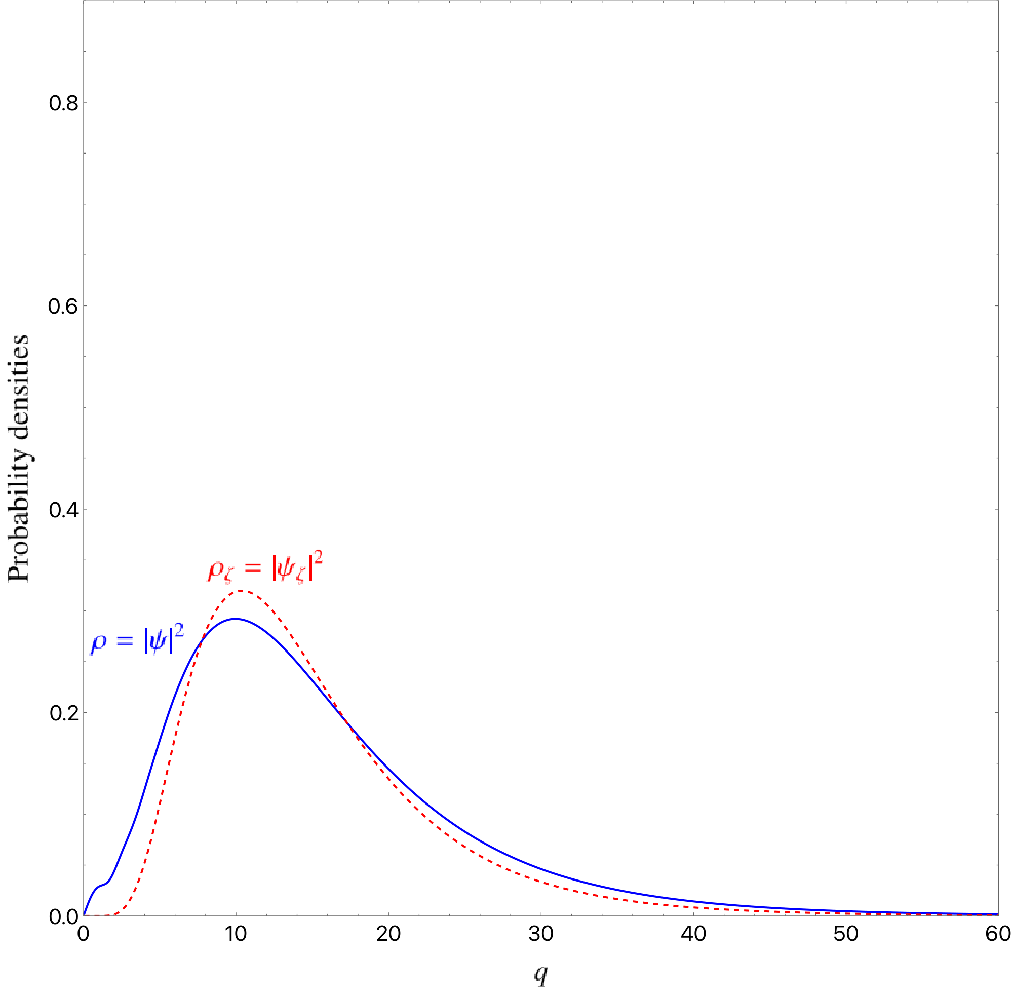
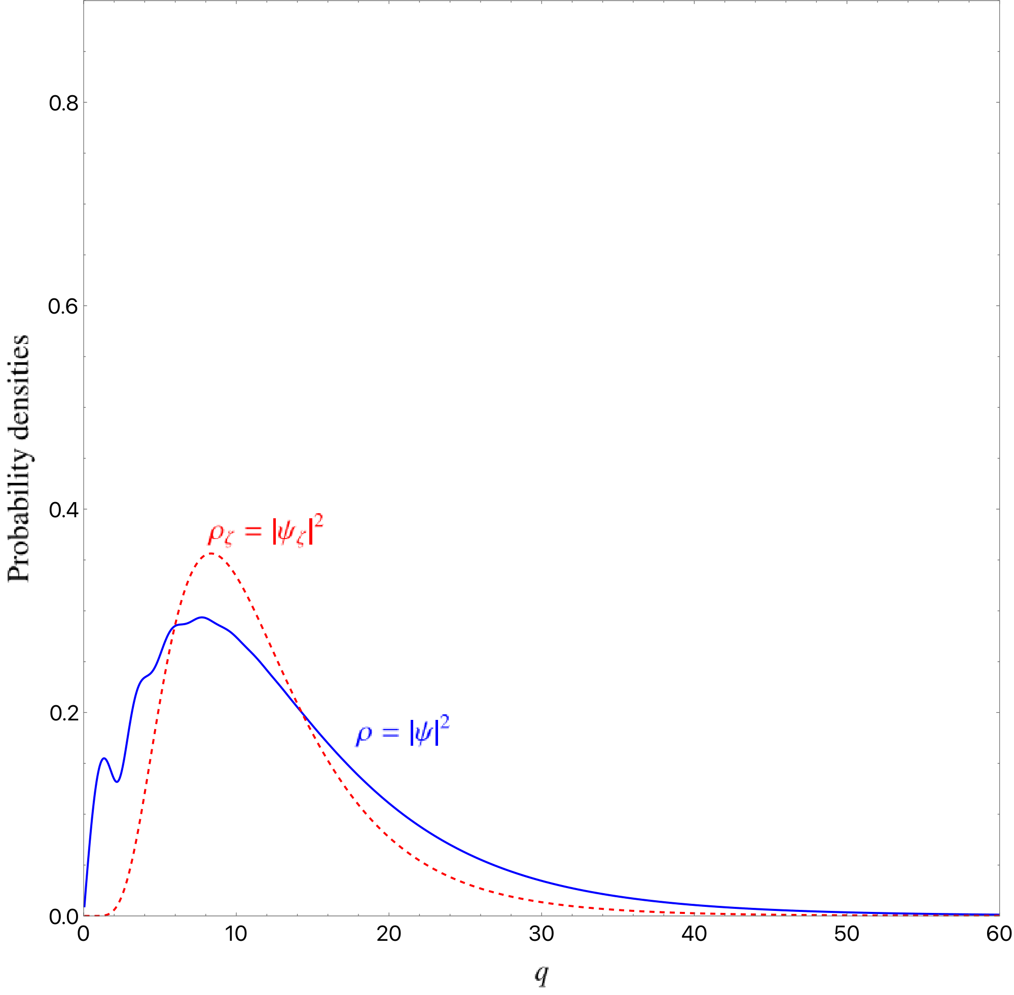
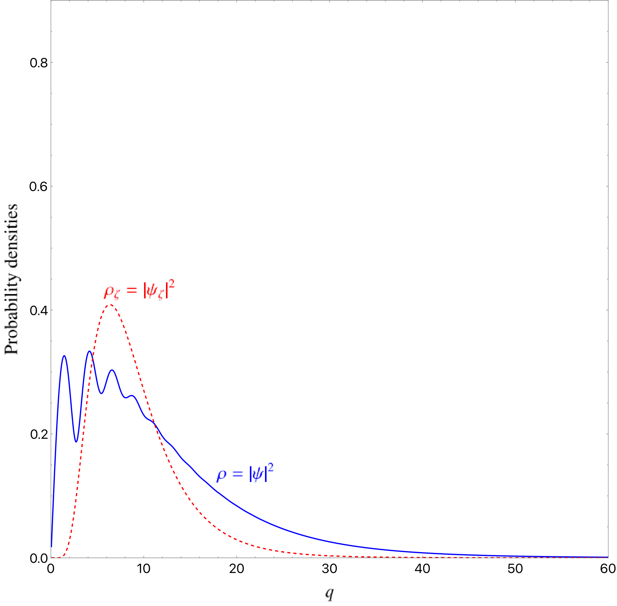
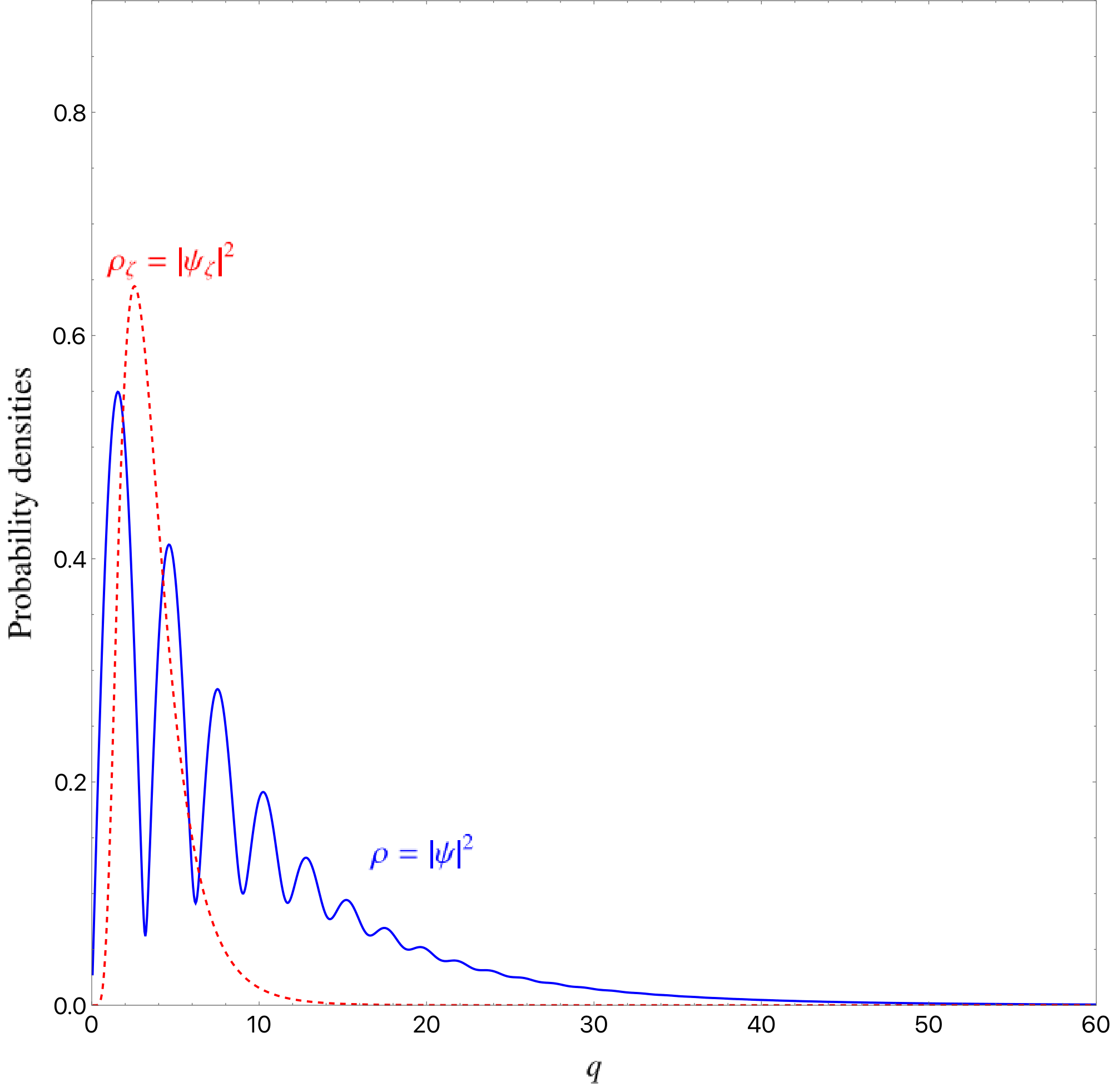
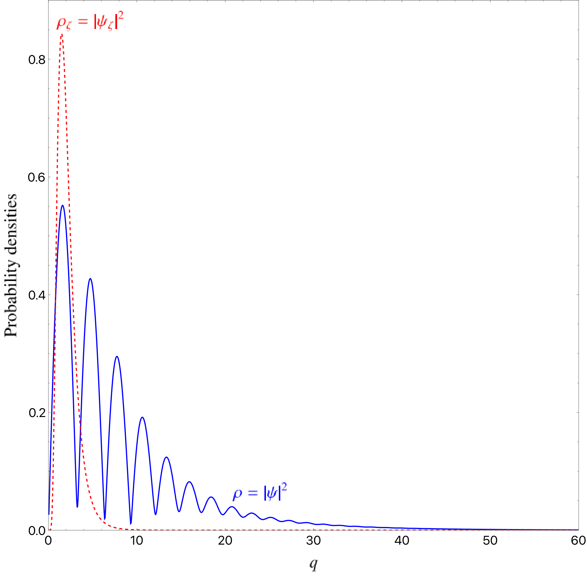
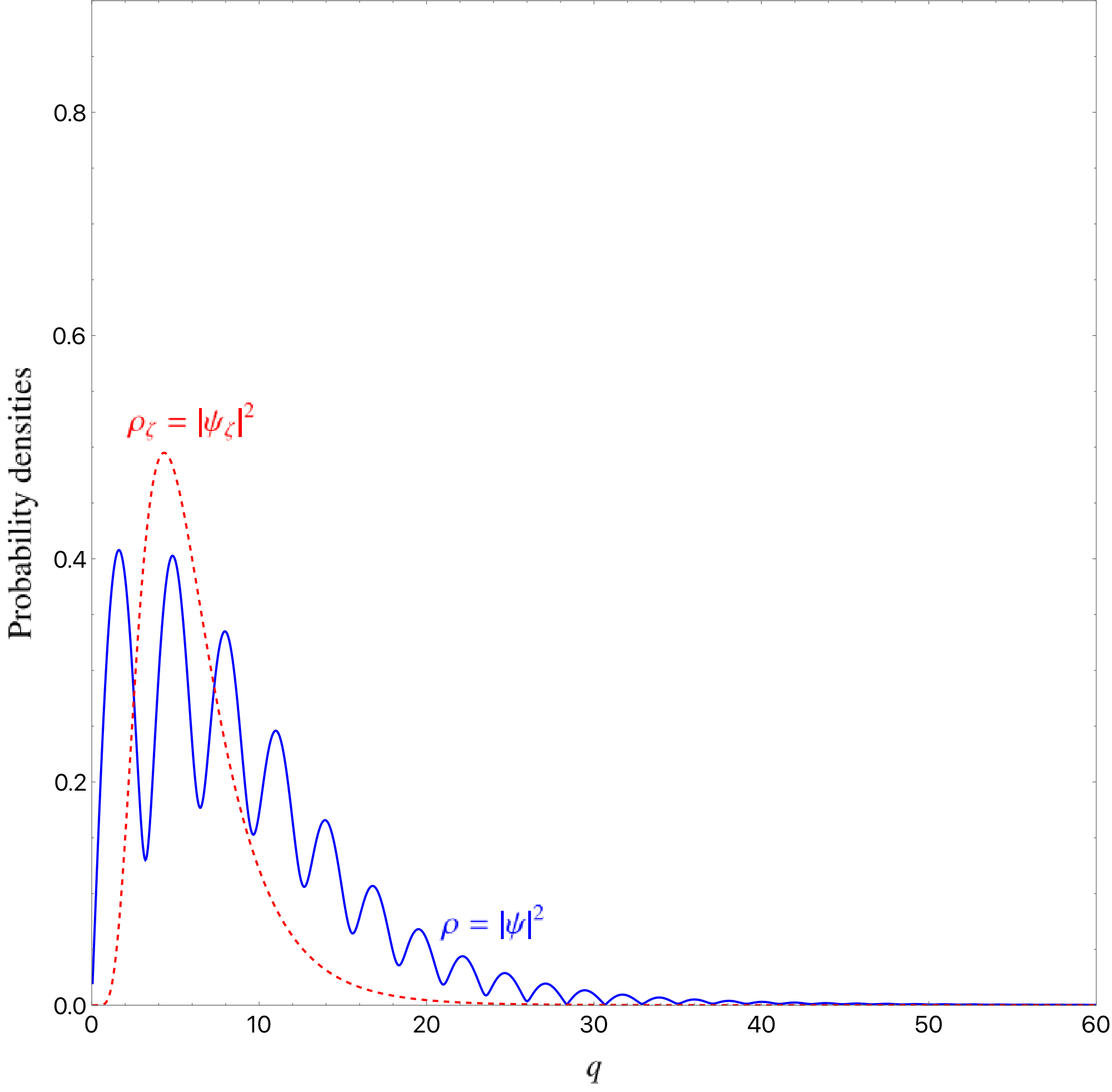
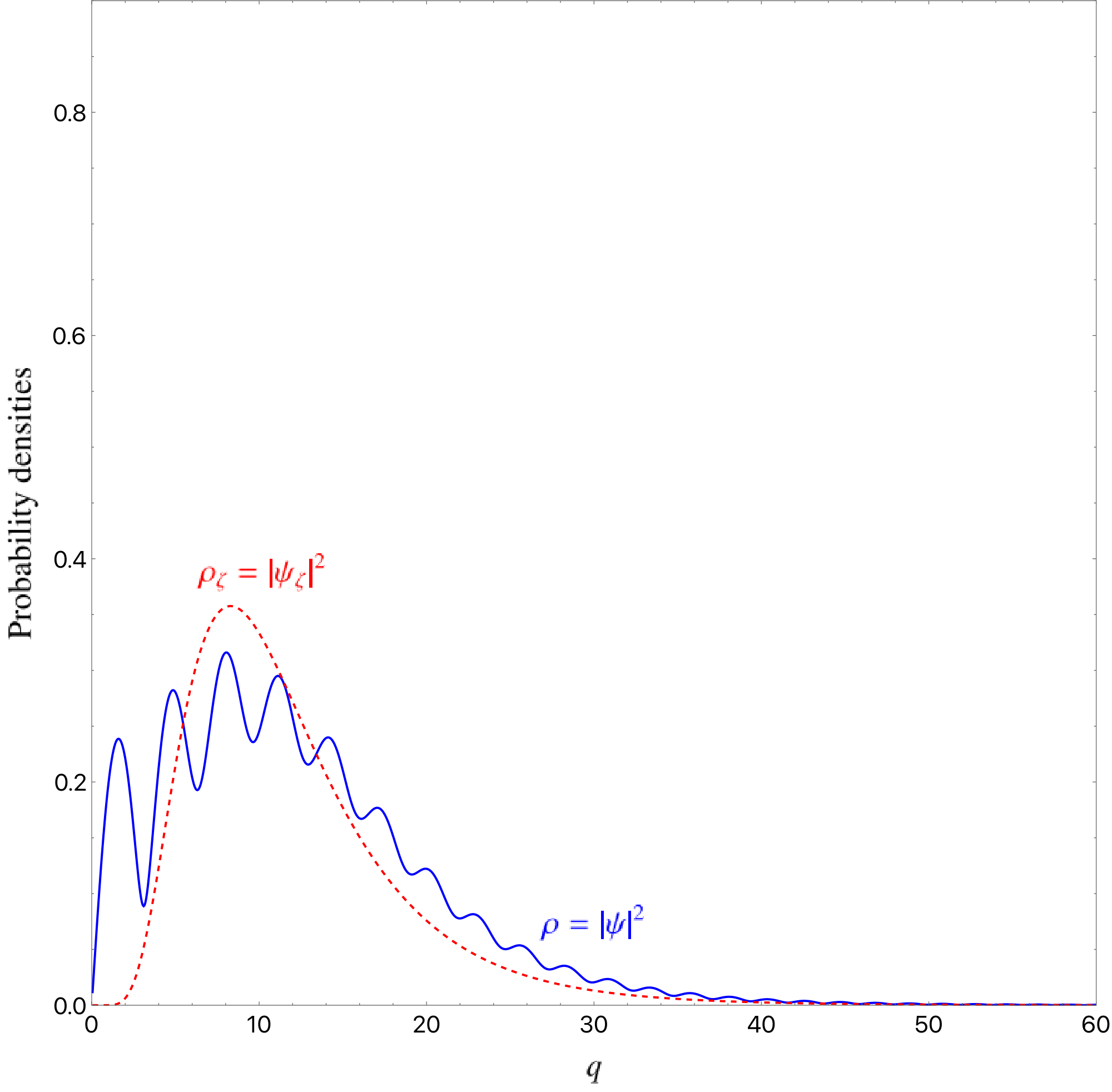
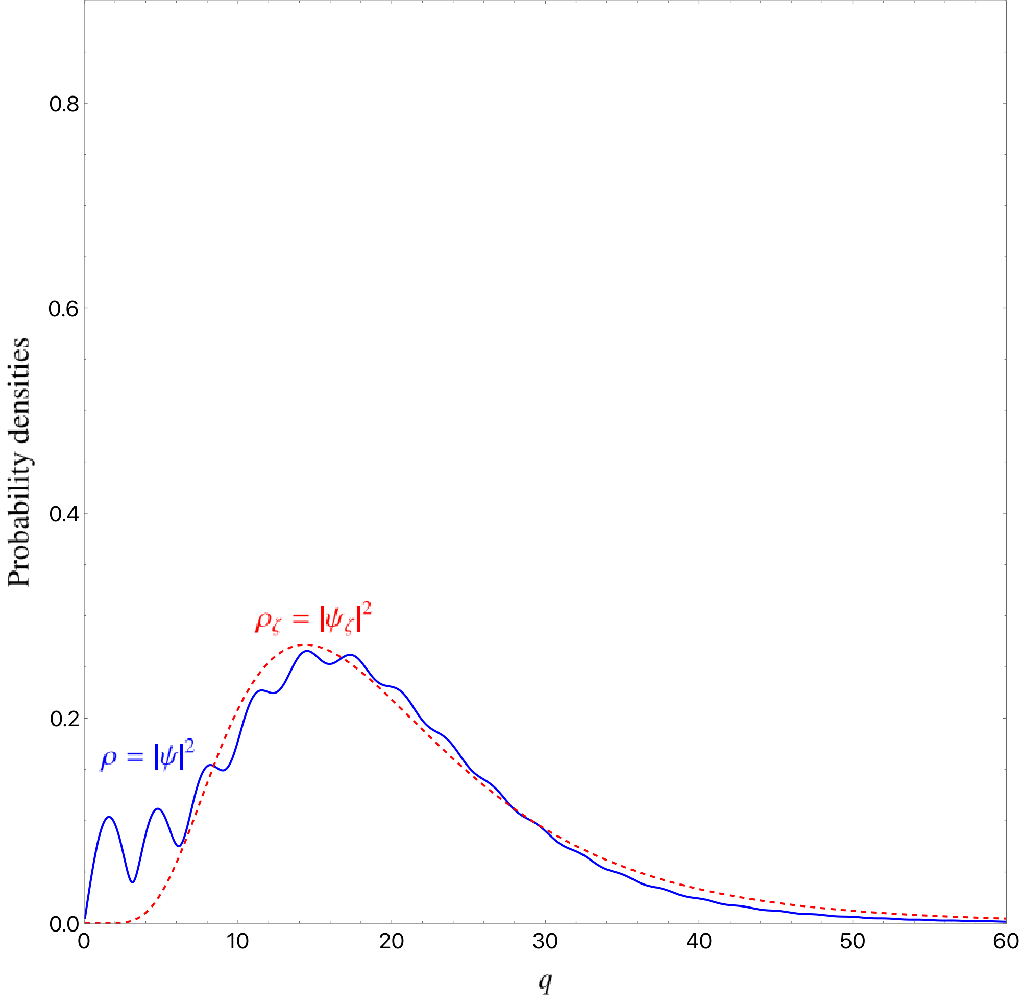
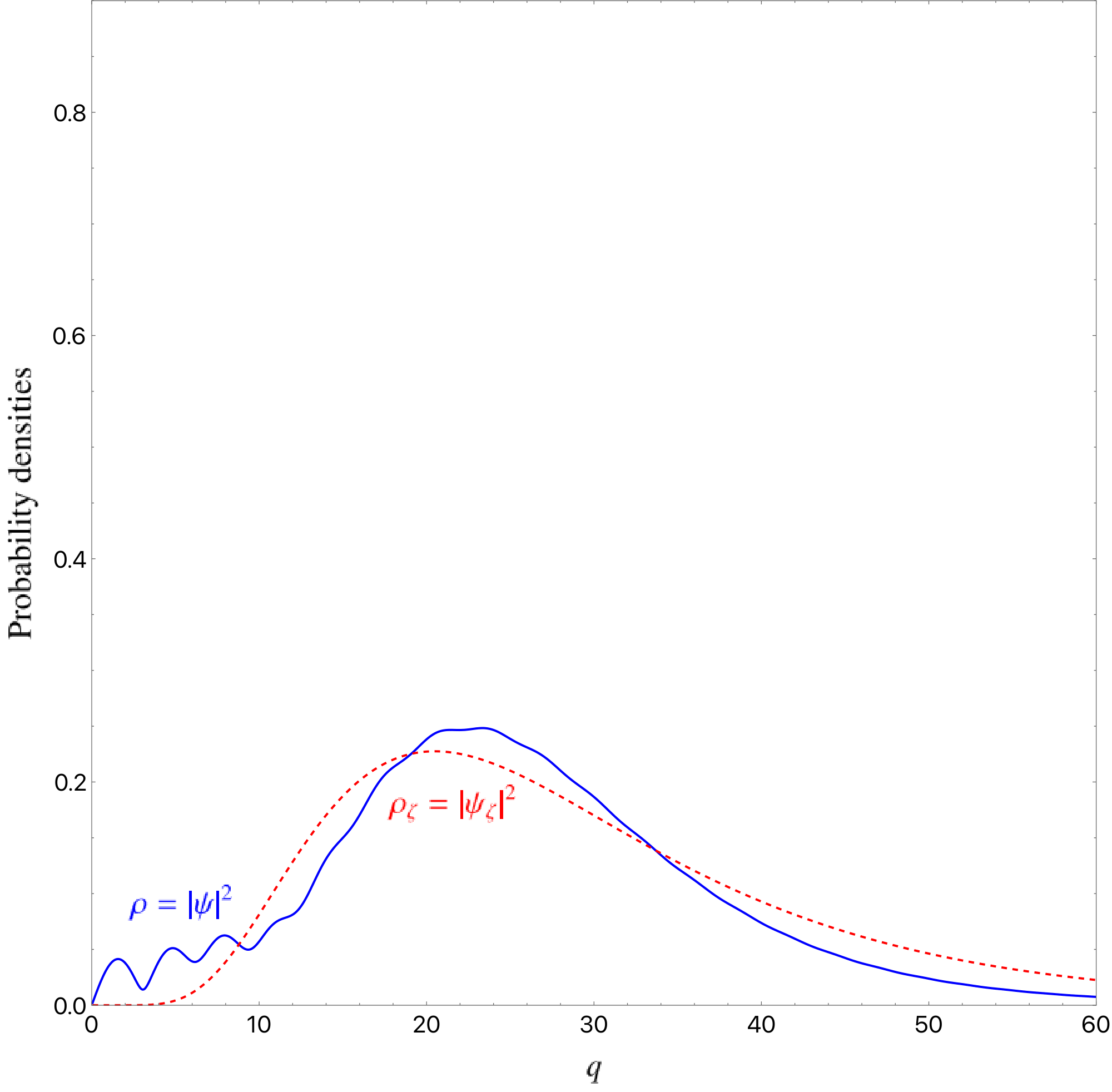
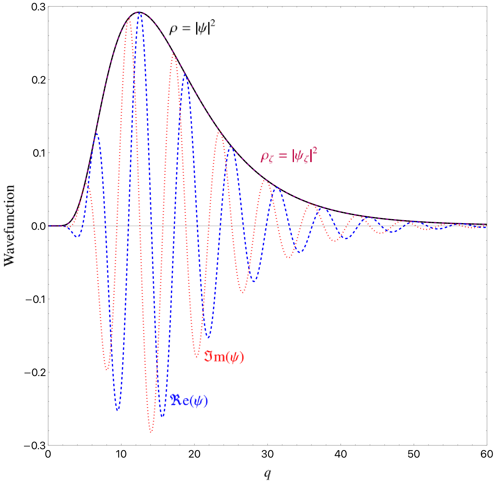
The more relevant model in which $\mathcal{K}\not=0$ can also be solved analytically under special conditions (see Ref. Małkiewicz et al. 2020 for details and the solution itself). Our choice in the present work was to assume an initial wavefunction $\psi_{\text{true}}(q,t_{\text{ini}})$ in the far past, with $q$ large, to be in a coherent state $\psi_{\zeta}(q,t_{\text{ini}})$ (see the right panel of Figure 3) and to evolve it with the Schrödinger equation. Figure 2 shows how $\psi(q,t)=\psi_{\text{true}}(q,t)$ and then very rapidly departs from $\psi_{\zeta}(q,t)$, although the expectation value trajectories $q_{\text{sem}}$ and $Q_{\text{sem}}$ remain similar (in shape, if not in actual values) to $q_{\zeta}$. As it happens, as the wave packets move towards the origin $q\to 0$, $\psi$ starts oscillating, thus producing the oscillations in the dBB trajectory $Q_{\text{d}\textsc{bb}}$, while the coherent state remains smooth at all times, being merely squeezed close to the origin. It is interesting to note that even though the wavefunctions differ drastically at the time of the bounce, the relevant trajectories (except the dBB one) are well described by (29), although with different parameters $q_{\textsc{b}}$ and $\omega$. We take that as an indication that the coherent state approximation is a valid one in most circumstances as long as one is only interested in expectation values. Given the very significant differences with the true wavefunction, however, it can be assumed that higher order moments are not well approximated.

As a result, the trajectories defined through either expectation values or coherent state approximation are invariant under the clock transformation (24), contrary to the dBB ones. However, as can be seen on Figure 4, in which the transformation stemming from the free particle Hamiltonian is applied to the phase space trajectories, they do depend on the choice of clock before quantisation. This is actually even more true for the dBB case, for which these clock transformations can lead to such tremendous modifications of the space space trajectories that the actual predictivity of the underlying theory becomes questionable.

We have reviewed the question of clock transformation and trajectories in quantum cosmology by means of a simple deparametrised and quantised Bianchi I model. The Wheeler–DeWitt equation in this minisuperspace case reduces to the Schrödinger equation of a free particle or, depending on the quantisation scheme, with a repulsive potential which can be studied using standard techniques. The relevant degree of freedom, from the point of view of cosmology, is the spatial volume $q=V$, i.e., the cube of the scale factor $a$, while the canonically conjugate momentum is mostly given by the Hubble parameter.

Extending a previous work Małkiewicz et al. 2020 to include dBB trajectories, we found very substantial differences between those and their counterparts obtained by some averaging processes. In the later case, all trajectories stem from a semiclassical Hamiltonian and are therefore invariant under the corresponding clock transformation (although not for that corresponding to the original classical theory). In the former case, however, unless the wavefunction is restricted to belong to a very special class (for which the coherent state approximation is not valid), we found that the dBB trajectories depend in a much more drastic way on the clock transformations, rendering the ambiguity it stems from extremely serious, to the point that the theory may no longer even be predictive. Calculating the spectrum of primordial perturbations, for instance, involves the second time derivative of the scale factor, and hence of our $q$, so that the choice of clock and initial conditions can yield tremendously different predictions. For semiclassical trajectories, on the other hand, the choice is mostly irrelevant, and the resulting perturbations might merely depend on a few parameters.

That said, it must be emphasised that the classical limit is, in all cases (hence including dBB), well defined and consistent, so there remains the possibility that whatever dynamical quantity (e.g., perturbations) is evolved through the full quantum phase might be unique. We postpone such a discussion to a forthcoming work Boldrin et al. 2022.

This research was funded by the Polish National Agency for Academic Exchange and Programme Hubert Curien POLONIUM 2019 grant number 42657QJ.

References

- Anderson (2017) Anderson, E. The Problem of Time; Springer: Cham, Switzerland, 2017; Volume 190.
- Kiefer and Peter (2022) Kiefer, C.; Peter, P. Time in quantum cosmology. Universe 2022, 8, 36,
- Małkiewicz et al. (2020) Małkiewicz, P.; Peter, P.; Vitenti, S.D.P. Quantum empty Bianchi I spacetime with internal time. Phys. Rev. D 2020, 101, 046012,
- Martin et al. (2021) Martin, J.d.C.; Małkiewicz, P.; Peter, P. Unitarily inequivalent quantum cosmological bouncing models. Phys. Rev. D 2022, 105, 023522,
- Vilenkin (1988) Vilenkin, A. Quantum Cosmology and the Initial State of the Universe. Phys. Rev. D 1988, 37, 888.
- Małkiewicz (2015) Małkiewicz, P. Multiple choices of time in quantum cosmology. Class. Quant. Grav. 2015, 32, 135004,
- Małkiewicz and Miroszewski (2017) Małkiewicz, P.; Miroszewski, A. Internal clock formulation of quantum mechanics. Phys. Rev. D 2017, 96, 046003,
- Klauder (2015) Klauder, J.R. Enhanced Quantization: Particles, Fields and Gravity; World Scientific: Hackensack, NJ, USA, 2015.
- Holland (1993) Holland, P.R. The de Broglie-Bohm theory of motion and quantum field theory. Phys. Rept. 1993, 224, 95–150.
- de Broglie (1927) De Broglie, L. La mécanique ondulatoire et la structure atomique de la matière. J. Phys. Radium 1927, 8, 225–241.
- Bohm (1952a) Bohm, D. A Suggested interpretation of the quantum theory in terms of hidden variables. 1. Phys. Rev. 1952, 85, 166–179.
- Bohm (1952b) Bohm, D. A Suggested interpretation of the quantum theory in terms of hidden variables. 2. Phys. Rev. 1952, 85, 180–193.
- Kiefer (2012) Kiefer, C. Quantum Gravity, 3rd ed.; Oxford University Press: Oxford, UK, 2012.
- Pinto-Neto and Fabris (2013) Pinto-Neto, N.; Fabris, J.C. Quantum cosmology from the de Broglie-Bohm perspective. Class. Quant. Grav. 2013, 30, 143001,
- Acacio de Barros et al. (1998) Acacio de Barros, J.; Pinto-Neto, N.; Sagioro-Leal, M.A. The Causal interpretation of dust and radiation fluids nonsingular quantum cosmologies. Phys. Lett. 1998, A241, 229–239,
- Boldrin et al. (2022) Boldrin, A.; Małkiewicz, P.; Peter, P. Problem of time and the generation of primordial structure. 2022, in preparation.