跳到论文正文
W Papers独立论文阅读器 arXiv:2201.09098 论文正文 计算阅读时间 · 0%
引用这篇论文根据当前论文元数据生成,正式投稿前建议核对。


License: CC BY 4.0
arXiv:2201.09098v2 [stat.ME] 17 May 2022

Estimation of the covariance structure from SNP allele frequencies

Jan van Waaij1, Zilong Li2, Carsten Wiuf1,∗

∗ Corresponding author (wiuf@math.ku.dk)

Running title: Estimation of SNP Covariance Matrix

1 Department of Mathematical Science, University of Copenhagen, 2100 Copenhagen, Denmark

2 Department of Biology, University of Copenhagen, 2100 Copenhagen, Denmark

Abstract

We propose two new statistics, V^\widehat{V} and S^\widehat{S}, to disentangle the population history of related populations from SNP frequency data. If the populations are related by a tree, we show by theoretical means as well as by simulation that the new statistics are able to identify the root of a tree correctly, in contrast to standard statistics, such as the observed matrix of F2F_{2}-statistics (distances between pairs of populations). The statistic V^\widehat{V} is obtained by averaging over all SNPs (similar to standard statistics). Its expectation is the true covariance matrix of the observed population SNP frequencies, offset by a matrix with identical entries. In contrast, the statistic S^\widehat{S} is put in a Bayesian context and is obtained by averaging over pairs of SNPs, such that each SNP is only used once. It thus makes use of the joint distribution of pairs of SNPs.

In addition, we provide a number of novel mathematical results about old and new statistics, and their mutual relationship.

1 Introduction

A common situation in population genetics is ancestral disentanglement of related populations (Pickrell and Pritchard 2012, Patterson et al. 2012, Leppala et al. 2017, Lipson 2020, Korunes and Goldberg 2021). Imagine we observe genetic data in the form of allele frequencies from nn SNPs and mm related populations, and assume the population history is described by an unknown admixture graph. This graph is estimated from the data under the assumption of neutral evolution. The estimation typically takes place in two steps. First the covariance matrix of the SNP allele frequencies is estimated from the data, which in turn is used to determine the admixture graph. This covariance matrix is at the core of much inference on population history. In this article we are interested in efficient estimation of the covariance matrix.

To put some notation, assume we observe data vectors, X1,…,XnX^{1},\ldots,X^{n} (one for each SNP), where Xk=(X1k,…,Xmk)tX^{k}=(X_{1}^{k},\ldots,X_{m}^{k})^{t} is an mm-dimensional real-valued vector with common expectations 𝔼⁡(Xik)=μk\E(X_{i}^{k})=\mu_{k}, i=1,…,mi=1,\ldots,m, and m×mm\times m covariance matrix Σk\Sigma^{k}, k=1,…,nk=1,\ldots,n. Here, XjkX_{j}^{k} is the frequency of a particular allele (say, the reference allele) of the kkth SNP in population jj. While it is standard to assume an underlying admixture graph or tree (Patterson et al. 2012, Lipson 2020), we will not impose this here. However, we do assume the populations share a common ancestor (‘root’) at some point in the past, represented by the mean value μk\mu_{k}.

The objective is to estimate

Σ=1n​∑k=1nΣk=1n​∑k=1n𝔼⁡[(Xk−μk​e)​(Xk−μk​e)t],\Sigma=\frac{1}{n}\sum_{k=1}^{n}\Sigma^{k}=\frac{1}{n}\sum_{k=1}^{n}\E[(X^{k}-\mu_{k}e)(X^{k}-\mu_{k}e)^{t}], (1)

the average covariance matrix over all sites. The mean values μk\mu_{k}, k=1,…,nk=1,\ldots,n, are nuisance parameters of little interest. In the absence of any knowledge about μk\mu_{k}, Pickrell and Pritchard 2012 suggests a surrogat statistic W^\widehat{W} for a related covariance matrix WW, obtained from Σ\Sigma by replacing μk\mu_{k} in eq. 1 with the average allele frequency. If the population history is a tree, one cannot infer the placement of the root from W^\widehat{W}. Consequently, to rectify this, one might choose manually one population as an outgroup and use this to place the root (Pickrell and Pritchard 2012). The same situation appears for another surrogate statistic, the observed distance matrix D^\widehat{D}, that is an estimator of the pairwise F2F_{2}-distance matrix DD (for formal definitions, see section 2) (Patterson et al. 2012).

In the present paper, we are concerned with two things. The first is to make available some results on the statistics W^\widehat{W} and D^\widehat{D}, and their mutual relationship. The second is to propose two new statistics, V^\widehat{V} and S^\widehat{S}, that both can be used to recover the placement of the root, without using an outgroup. Whereas, V^\widehat{V} is similar in spirit to W^\widehat{W} and D^\widehat{D} in the sense of averaging over all SNPs, S^\widehat{S} is based on pairwise comparison of SNPs, and is put in a Bayesian context. This statistic might open for new ways to explore the data.

The results are stated generally and do not rely on any specific distributional assumptions on the SNP allele frequencies. In particular, the XikX_{i}^{k}s do not need to be frequencies at all, but could be arbitrary random variables with mean and variance. Hence, the proposed theory and methodology might have wider applications in population genetics and genomics, as well as outside these fields.

Notation

If AA is a matrix, then AtA^{t} denotes the transposed matrix. Vectors are assumed to be column vectors. If vv is a vector, then vtv^{t} is a row vector. Let II be the m×mm\times m identity matrix, EE the symmetric m×mm\times m square matrix with all entries equal to one, and e=(1,…,1)te=(1,\ldots,1)^{t} the vector in ℝm\R^{m} with all entries one. Furthermore, let eie_{i} be the iith unit vector, i=1,…,mi=1,\ldots,m. So, (ei)i=1(e_{i})_{i}=1 and (ei)j=0(e_{i})_{j}=0 for j≠ij\neq i.

For an m​×⁡mm\x m matrix AA, the Frobenius norm of AA is ‖A‖F=∑a=1m∑b=1mAa​b2\|A\|_{F}=\sqrt{\sum_{a=1}^{m}\sum_{b=1}^{m}A_{ab}^{2}}. For a linear operator 𝒳:𝕊m→𝕊m\sX\colon\mathbb{S}_{m}\to\mathbb{S}_{m}, the image is im⁡(𝒳)={𝒳⁡(A):A∈𝕊m}\im(\sX)=\left\{\sX(A)\colon A\in\mathbb{S}_{m}\right\}, and the operator norm is

‖𝒳‖op=sup‖A‖F=1‖𝒳⁡(A)‖F.\|\sX\|_{\text{op}}=\sup_{\|A\|_{F}=1}\|\sX(A)\|_{F}.

If 𝒳\sX is an orthogonal projection then the operator norm is one.

2 Estimation of the covariance matrix

The theory to be developed holds for general random vectors, X1,…,XnX^{1},\ldots,X^{n} with values in ℝm\R^{m}, m≥2m\geq 2. However, we put the theory in the context of population genetics as this is the application area we have in mind. Thus, we think of Xk=(X1k,…,Xmk)X^{k}=(X_{1}^{k},\ldots,X^{k}_{m}), k=1,…,nk=1,\ldots,n, as vectors of observed allele frequencies, either population or sample based.

Recall the covariance matrix in eq. 1,

Σ=1n​∑k=1nΣk=1n​∑k=1n𝔼⁡[(Xk−μk​e)​(Xk−μk​e)t].\Sigma=\frac{1}{n}\sum_{k=1}^{n}\Sigma^{k}=\frac{1}{n}\sum_{k=1}^{n}\E[(X^{k}-\mu_{k}e)(X^{k}-\mu_{k}e)^{t}].

In the case the means μk\mu_{k}, k=1,…,nk=1,\ldots,n, are known, then a natural unbiased estimator of Σ=(Σi​j)i,j=1,…,m\Sigma=(\Sigma_{ij})_{i,j=1,\ldots,m}, is

Σ^i​j=1n​∑k=1n(Xik−μk)​(Xjk−μk),i,j=1,…,m.\widehat{\Sigma}_{ij}=\frac{1}{n}\sum_{k=1}^{n}(X_{i}^{k}-\mu_{k})(X_{j}^{k}-\mu_{k}),\quad i,j=1,\ldots,m. (2)

However, in the absence of such knowledge, we cannot estimate Σ\Sigma from the data without further assumptions. This has led to the proposal of alternative approaches, for example by substitution of μk\mu_{k} with an estimated mean (Pickrell and Pritchard 2012). A natural unbiased estimator of μk\mu_{k} is the moment estimator 1m​∑i=1mXik\frac{1}{m}\sum_{i=1}^{m}X_{i}^{k}. Plugging this into eq. 2, yields the statistic W^\widehat{W} given by

W^i​j=1n​∑k=1n(Xik−μ^k)​(Xjk−μ^k),whereμ^k=1m​∑i=1mXik\widehat{W}_{ij}=\frac{1}{n}\sum_{k=1}^{n}\left(X_{i}^{k}-\widehat{\mu}_{k}\right)\left(X_{j}^{k}-\widehat{\mu}_{k}\right),\quad\text{where}\quad\widehat{\mu}_{k}=\frac{1}{m}\sum_{i=1}^{m}X_{i}^{k}

is the empirical mean (Pickrell and Pritchard 2012). This is not an estimator of Σ\Sigma per se, but it still contains information about the data generating process. In Pickrell and Pritchard 2012, W^\widehat{W} is used as a surrogate for Σ^\widehat{\Sigma}.

Obviously, W^\widehat{W} is a symmetric matrix and

W^i​j\displaystyle\widehat{W}_{ij} =1n​∑k=1n((Xik−μk)−1m​∑a=1m(Xak−μk))​((Xjk−μk)−1m​∑b=1m(Xbk−μk))\displaystyle=\frac{1}{n}\sum_{k=1}^{n}\left((X_{i}^{k}-\mu_{k})-\frac{1}{m}\sum_{a=1}^{m}(X_{a}^{k}-\mu_{k})\right)\left((X_{j}^{k}-\mu_{k})-\frac{1}{m}\sum_{b=1}^{m}(X_{b}^{k}-\mu_{k})\right)
=Σ^i​j−1m​∑a=1mΣ^i​a−1m​∑b=1mΣ^j​b+1m2​∑a=1m∑b=1mΣ^a​b\displaystyle=\widehat{\Sigma}_{ij}-\frac{1}{m}\sum_{a=1}^{m}\widehat{\Sigma}_{ia}-\frac{1}{m}\sum_{b=1}^{m}\widehat{\Sigma}_{jb}+\frac{1}{m^{2}}\sum_{a=1}^{m}\sum_{b=1}^{m}\widehat{\Sigma}_{ab}

(Pickrell and Pritchard 2012, equation 23).

Patterson et al. 2012 suggest a different statistic to capture the evolutionary distances between the populations. For populations ii and jj, and SNP kk, the distance between the populations (at SNP kk) is defined as the variance of Xik−XjkX_{i}^{k}-X_{j}^{k}, which is known as an F2F_{2} statistic. Let DD be the matrix with (i,j)(i,j) entry Di​j=1n​∑k=1nvar⁡(Xik−Xjk)D_{ij}=\frac{1}{n}\sum_{k=1}^{n}\var(X_{i}^{k}-X_{j}^{k}). An obvious estimator of DD is defined by

D^i​j=1n​∑k=1n(Xik−Xjk)2.\widehat{D}_{ij}=\frac{1}{n}\sum_{k=1}^{n}(X_{i}^{k}-X_{j}^{k})^{2}.

Also, DD and D^\widehat{D} are symmetric matrices, and

D^i​j=1n​∑k=1n(Xik−μk+μk−Xjk)2=Σ^i​i+Σ^j​j−2​Σ^i​j.\widehat{D}_{ij}=\frac{1}{n}\sum_{k=1}^{n}(X_{i}^{k}-\mu_{k}+\mu_{k}-X_{j}^{k})^{2}=\widehat{\Sigma}_{ii}+\widehat{\Sigma}_{jj}-2\widehat{\Sigma}_{ij}.

Thus, both D^\widehat{D} and W^\widehat{W} are linear transformations of Σ^\widehat{\Sigma}. Furthermore, they are related to each other by an isomorphism (see theorem 2), and hence carry the same information. To formalise this, we need some further notation.

Let 𝕊m\mathbb{S}_{m} be the vector space of symmetric m​×⁡mm\x m-matrices with dimension m⁡(m+1)/2m(m+1)/2, and define linear operators 𝒟,𝒲:𝕊m→𝕊m\sD,\sW\colon\mathbb{S}_{m}\to\mathbb{S}_{m} by

𝒲⁡(A)ij=\displaystyle\sW(A)_{ij}= Ai​j−1m​∑a=1mAi​a−1m​∑a=1mAj​a+1m2​∑a=1m∑b=1mAa​b,\displaystyle A_{ij}-\frac{1}{m}\sum_{a=1}^{m}A_{ia}-\frac{1}{m}\sum_{a=1}^{m}A_{ja}+\frac{1}{m^{2}}\sum_{a=1}^{m}\sum_{b=1}^{m}A_{ab},
𝒟⁡(A)ij=\displaystyle\sD(A)_{ij}= Ai​i+Aj​j−2​Ai​j.\displaystyle A_{ii}+A_{jj}-2A_{ij}.

Obviously, D^=𝒟⁡(Σ^)\widehat{D}=\sD(\widehat{\Sigma}) and W^=𝒲⁡(Σ^)\widehat{W}=\sW(\widehat{\Sigma}).

Lemma 1.

The linear operator 𝒲\sW has the representation

𝒲⁡(A)=(I−1m​E)​A​(I−1m​E).\sW(A)=\left(I-\frac{1}{m}E\right)A\left(I-\frac{1}{m}E\right). (3)

Consequently, if AA is positive definite, then 𝒲⁡(A)\sW(A) is positive semi-definite. In particular, 𝒲⁡(Σ)\sW(\Sigma) is positive semi-definite.

Proof.

The first part follows by straightforward evaluation. For the second part, let x∈ℝmx\in\R^{m}. We have

xt​𝒲⁡(A)​x=xt​(I−1m​E)​A​(I−1m​E)​x=((I−1m​E)​x)t​A​(I−1m​E)​x≥0,\displaystyle x^{t}\sW(A)x=x^{t}\left(I-\tfrac{1}{m}E\right)A\left(I-\tfrac{1}{m}E\right)x=\left(\left(I-\tfrac{1}{m}E\right)x\right)^{t}A\left(I-\tfrac{1}{m}E\right)x\geq 0,

as AA is positive semi-definite by assumption. The final part follows by noting that Σ\Sigma is positive definite, since it is a covariance matrix. ∎

Theorem 2.

We have

𝒟=𝒟∘𝒲,𝒲=−12𝒲∘𝒟,𝒟∘𝒟=−2𝒟and𝒲∘𝒲=𝒲.\sD=\sD\circ\sW,\quad\sW=-\tfrac{1}{2}\sW\circ\sD,\quad\sD\circ\sD=-2\sD\en\sW\circ\sW=\sW.

The operator 𝒲\sW is an orthogonal projection (hence has operator norm one), while −12​𝒟-\frac{1}{2}\sD is a non-orthogonal projection with operator norm

‖−12​𝒟‖op=m.\|\!-\!\tfrac{1}{2}\sD\|_{\op}=\sqrt{m}.

The operators 𝒟\sD and 𝒲\sW have the same mm-dimensional kernel, given by

K\displaystyle K ={e​vt+v​et:v∈ℝm},\displaystyle=\left\{ev^{t}+ve^{t}\colon v\in\R^{m}\right\},

The restrictions

𝒲:im⁡(𝒟)→im⁡(𝒲),−12​𝒟:im⁡(𝒲)→im⁡(𝒟)\sW\colon\im(\sD)\to\im(\sW),\quad-\tfrac{1}{2}\sD\colon\im(\sW)\to\im(\sD)

are each others inverse. The images of 𝒲\sW and 𝒟\sD have dimension 12​m​(m−1)\tfrac{1}{2}m(m-1).

The proof of theorem 2 is deferred to section 7.1.

Let W:=𝔼⁡(W^)W:=\E(\widehat{W}) and D:=𝔼⁡(D^)D:=\E(\widehat{D}).

Theorem 3.

It holds that W=𝒲⁡(Σ)W=\sW(\Sigma), and D=𝒟⁡(Σ)D=\sD(\Sigma).

Proof.

By linearity of the expectation and the definition of 𝒲\sW and 𝒟\sD. ∎

The interpretation of the results are well understood in the case the populations are related by a tree, see fig. 1. In this case, it is standard to associate independent random variables to the edges and the root of the tree, such that

Xki=Ckr+∑e∈Γr​iCke,k=1,…,n,i=1,…,m,X^{k}_{i}=C^{k}_{r}+\sum_{e\in\Gamma_{ri}}C^{k}_{e},\quad k=1,\ldots,n,\quad i=1,\ldots,m, (4)

where the sum is over all edges ee on the unique path Γr​i\Gamma_{ri} from the root rr to population ii, CrkC^{k}_{r} is the random variable associated the root, and CekC^{k}_{e} the random variable associated the edge ee. This model naturally arises from the normal approximation model,

Xt∼Normal​(x0,tNe​x0​(1−x0))X_{t}\sim\text{Normal}\left(x_{0},\frac{t}{N_{e}}x_{0}(1-x_{0})\right)

(Nicholson et al. 2002), where x0x_{0} is the SNP frequency at time 00, NeN_{e} is the effective population size, and XtX_{t} is the SNP frequency tt generations later. The change in frequency might be found by summing independent increments over different time epochs, leading to the model in eq. 4.

Consider the case of m=2m=2, and let Σ\Sigma be given as

Σ=(σ1+τττσ2+τ),\Sigma=\begin{pmatrix}\sigma_{1}+\tau&\tau\\ \tau&\sigma_{2}+\tau\end{pmatrix}, (5)

where σ1,σ2,τ≥0\sigma_{1},\sigma_{2},\tau\geq 0, corresponding to the graph in fig. 1(a). Typically, in an evolutionary context, τ\tau might be taken to be zero (the variance of the root variable), as data from the two populations will not contain any information about the evolution of the two populations prior to their most recent common ancestor. However, one might alternatively think of τ\tau as the variance of the SNP means μk\mu_{k}, k=1,…,nk=1,\ldots,n (to be explored in section 5).

It follows from eq. 5 and D=𝒟⁡(Σ)D=\sD(\Sigma) that

𝒟⁡(Σ)=(0σ1+σ2σ1+σ20),\sD(\Sigma)=\begin{pmatrix}0&\sigma_{1}+\sigma_{2}\\ \sigma_{1}+\sigma_{2}&0\end{pmatrix},

from which only the sum σ1+σ2\sigma_{1}+\sigma_{2} might be recovered. Hence, neither the length of the “root tip” (τ\tau) nor the placement of the root can be recovered. The elements of the kernel might be seen as operations on the tree, while preserving 𝒟⁡(Σ)\sD(\Sigma). This is perhaps best illustrated for m=3m=3, in which case we take the tree of fig. 1(b) as starting point, with

Σ=(σ11000σ12+σ2σ120σ12σ12+σ3)+τ​E.\Sigma=\begin{pmatrix}\sigma_{11}&0&0\\ 0&\sigma_{12}+\sigma_{2}&\sigma_{12}\\ 0&\sigma_{12}&\sigma_{12}+\sigma_{3}\end{pmatrix}+\tau E.

Adding the kernel element

e​(y00)+(y00)​e′+(x−y)​E=x​E+(y000−y−y0−y−y)e\begin{pmatrix}y&0&0\end{pmatrix}+\begin{pmatrix}y\\ 0\\ 0\end{pmatrix}e^{\prime}+(x-y)E=xE+\begin{pmatrix}y&0&0\\ 0&-y&-y\\ 0&-y&-y\end{pmatrix}

to Σ\Sigma corresponds to extending the outgoing edge from the root with xx and sliding the root by yy to the right on the edge, see fig. 1(b) and (c). Choosing y=σ12y=\sigma_{12} yields a trifurcated star-shaped tree. Now, using other similar kernel elements, the star-shaped tree might be turned into many other trees while preserving the distance matrix

𝒟⁡(Σ)=(0σ1+σ2σ1+σ3σ1+σ20σ2+σ3σ1+σ3σ2+σ30),\displaystyle\sD(\Sigma)=\begin{pmatrix}0&\sigma_{1}+\sigma_{2}&\sigma_{1}+\sigma_{3}\\ \sigma_{1}+\sigma_{2}&0&\sigma_{2}+\sigma_{3}\\ \sigma_{1}+\sigma_{3}&\sigma_{2}+\sigma_{3}&0\end{pmatrix},

where σ11+σ12=σ1\sigma_{11}+\sigma_{12}=\sigma_{1}.

The same applies for higher m>3m>3 by iteratively applying kernel matrices to move ancestral nodes of the tree while preserving 𝒟⁡(Σ)\sD(\Sigma).

Refer to caption
Figure 1: A tree with two (a) and three (b) leaves. In (c), the length τ\tau of the root tip is extended by xx and slided yy to the right. We refer to the full edge labelled tree as a rooted tree with a root tip; the tree without the root tip but with the placement of the root as a rooted tree without the root tip; and the tree without the root tip and the placement of the root as an unrooted tree. In the latter case, the branches labeled σ11\sigma_{11} and σ1\sigma_{1} in (b) are replaced by a single branch of length σ11+σ12\sigma_{11}+\sigma_{12}.

3 A new statistic

We suggest a third symmetric statistic, that carries more information about Σ\Sigma than the other two statistics. It is defined by

V^\displaystyle\widehat{V} =1n​∑k=1nXk​(Xk)t−μ^k2​E.\displaystyle=\frac{1}{n}\sum_{k=1}^{n}X^{k}(X^{k})^{t}-\widehat{\mu}_{k}^{2}E.

The second term is a correction term that makes the expectation of V^\widehat{V} independent of the mean μk\mu_{k}. Also, it ensures the sum of all entries of V^\widehat{V} is zero. In contrast to the other two statistics, V^\widehat{V} is not linear in Σ^\widehat{\Sigma}. However, if we define Y=1n​∑k=1nXk​(Xk)tY=\frac{1}{n}\sum_{k=1}^{n}X^{k}(X^{k})^{t}, then W^=𝒲⁡(Y)\widehat{W}=\sW(Y), D^=𝒟⁡(Y)\widehat{D}=\sD(Y) and V^=𝒱⁡(Y)\widehat{V}=\sV(Y), where VV is defined in eq. 6.

By inspection, it holds that 𝒲⁡(V^)=W^\sW(\widehat{V})=\widehat{W} and 𝒟⁡(V^)=D^\sD(\widehat{V})=\widehat{D}. Let 𝒱:𝕊m→𝕊m\sV\colon\mathbb{S}_{m}\to\mathbb{S}_{m} be defined as

𝒱⁡(A)=A−1m2​EAE.\sV(A)=A-\frac{1}{m^{2}}EAE. (6)

The following holds.

Theorem 4.

The operator 𝒱\sV is an orthogonal projection, 𝒱=𝒱∘𝒱\sV=\sV\circ\sV with kernel {λ​E:λ∈ℝ}\left\{\lambda E\colon\lambda\in\R\right\}. In particular, 𝒱\sV has operator norm one. Furthermore, V:=𝔼⁡(V^)=𝒱⁡(Σ)V:=\E(\widehat{V})=\sV(\Sigma).

Proof.

Let V=𝒱⁡(A)V=\sV(A). Note that et​V​e=0e^{t}Ve=0. Hence, 𝒱⁡(V)=V\sV(V)=V, which implies 𝒱∘𝒱=𝒱\sV\circ\sV=\sV. It follows from eq. 6, that 𝒱⁡(E)=0\sV(E)=0, but also that AA differs from 𝒱⁡(A)\sV(A) by a constant times EE. Hence ker⁡(𝒱)={λ​E:λ∈ℝ}\ker(\sV)=\left\{\lambda E:\lambda\in\R\right\}. Note that an m​×⁡mm\x m-matrix FF is orthogonal to EE if and only if ∑i=1m∑j=1mFi​j=0\sum_{i=1}^{m}\sum_{j=1}^{m}F_{ij}=0. We have

∑i=1m∑j=1m𝒱⁡(A)ij=∑i=1m∑j=1mAij−∑i=1m∑j=1mAij=0.\sum_{i=1}^{m}\sum_{j=1}^{m}\sV(A)_{ij}=\sum_{i=1}^{m}\sum_{j=1}^{m}A_{ij}-\sum_{i=1}^{m}\sum_{j=1}^{m}A_{ij}=0.

Hence, 𝒱\sV is an orthogonal projection. In particular, 𝒲\sW has operator norm one, for m≥2m\geq 2. Define V^k=Xk​(Xk)t−μ^k2​E\widehat{V}^{k}=X^{k}(X^{k})^{t}-\hat{\mu}_{k}^{2}E, such that V^=1n​∑k=1nV^k\widehat{V}=\frac{1}{n}\sum_{k=1}^{n}\widehat{V}^{k}. Note that

𝔼⁡(μ^k2)=1m2​∑a=1m∑b=1m𝔼⁡(Xak​Xbk)​and​𝔼⁡(Xk​(Xk)t)=Σk+μk2​E,\displaystyle\E(\hat{\mu}_{k}^{2})=\frac{1}{m^{2}}\sum_{a=1}^{m}\sum_{b=1}^{m}\E(X_{a}^{k}X_{b}^{k})\en\E(X^{k}(X^{k})^{t})=\Sigma^{k}+\mu_{k}^{2}E,

Then, 𝔼⁡(μ^k2)=μk2+et​Σk​e/(m2)\E(\hat{\mu}_{k}^{2})=\mu_{k}^{2}+e^{t}\Sigma^{k}e/(m^{2}), and

𝔼⁡(V^)=1n​∑k=1nΣk−1m2​(et​Σk​e)​E=Σ−1m2​E​Σ​E,\displaystyle\E(\widehat{V})=\frac{1}{n}\sum_{k=1}^{n}\Sigma^{k}-\frac{1}{m^{2}}(e^{t}\Sigma^{k}e)E=\Sigma-\frac{1}{m^{2}}E\Sigma E,

and the proof is complete. ∎

In the case of a tree, the placement of the root is identifiable from V=𝒱⁡(Σ)V=\sV(\Sigma), but not the length of the root tip. For m=2m=2, we find

𝒱⁡(Σ)=14​(3​σ1−σ2−σ1−σ2−σ1−σ23​σ2−σ1),\sV(\Sigma)=\frac{1}{4}\begin{pmatrix}3\sigma_{1}-\sigma_{2}&-\sigma_{1}-\sigma_{2}\\ -\sigma_{1}-\sigma_{2}&3\sigma_{2}-\sigma_{1}\end{pmatrix}, (7)

from which σ1,σ2\sigma_{1},\sigma_{2} might be recovered. The general statement for arbitrary mm is here:

Theorem 5.

The unrooted tree is identifiable from DD (or WW). The rooted tree without the root tip is identifiable from VV. The rooted tree with the root tip is identifiable from Σ\Sigma.

Proof.

The first statement is well known in literature (Semple and Steel, theorem 7.1.8, page 148). By theorem 2, it also holds true for WW.

Let 𝒯1=(𝒱1,ℰ1)\sT_{1}=(\sV_{1},\sE_{1}) and 𝒯2=(𝒱2,ℰ2)\sT_{2}=(\sV_{2},\sE_{2}) be two rooted trees with vertex sets 𝒱1,𝒱2\sV_{1},\sV_{2}, respectively, and edge sets ℰ1\sE_{1}, ℰ2\sE_{2}, respectively, and common m×mm\times m covariance matrix Σ\Sigma,. Define the (m+1)​×⁡(m+1)(m+1)\x(m+1) matrix AA as follows

(⋱Σ11𝒟⁡(Σ)⋱Σm​mΣ11…Σm​m0).\begin{pmatrix}\ddots&&&&\Sigma_{11}\\ &\sD(\Sigma)&&&\vdots\\ &&\ddots&&\Sigma_{mm}\\ \Sigma_{11}&\ldots&\Sigma_{mm}&&0\\ \end{pmatrix}.

The element Ai​jA_{ij} is the distance between the leaves ii and jj of 𝒯1\sT_{1} (or 𝒯2\sT_{2}) for i,j≤mi,j\leq m, and Ai,m+1=Am+1,i=Σi​iA_{i,m+1}=A_{m+1,i}=\Sigma_{ii} is the distance from the root to the leaf ii. If we consider the root as another ‘leaf’, then there is a isomorphism φ:𝒱1→𝒱2\varphi\colon\sV_{1}\to\sV_{2}, such that x−yx-y is an edge in 𝒱1\sV_{1} if and only if φ⁡(x)−φ⁡(y)\varphi(x)-\varphi(y) is an edge in 𝒯2\sT_{2} (indifferent of the direction). Moreover, the length of x−yx-y is equal to the length of φ⁡(x)−φ⁡(y)\varphi(x)-\varphi(y), and φ\varphi maps the iith leaf of 𝒯1\sT_{1} to the iith leaf of 𝒯2\sT_{2}, and the root of 𝒯1\sT_{1} to the root of 𝒯2\sT_{2}. It follows that 𝒯1\sT_{1} and 𝒯2\sT_{2} are isomorphic as directed labelled trees.

Let 𝒯1\sT_{1} and 𝒯2\sT_{2} be two trees with the same matrix VV. Let Σ1\Sigma_{1} and Σ2\Sigma_{2} be their corresponding covariance matrices. Then, Σ1−Σ2=λ​E\Sigma_{1}-\Sigma_{2}=\lambda E for some λ\lambda. Without loss of generality, λ≥0\lambda\geq 0. If we make the root tip of 𝒯2\sT_{2} λ\lambda longer, resulting in a tree 𝒯2′\sT_{2}^{\prime}, with corresponding covariance matrix Σ2′\Sigma_{2}^{\prime}, then Σ1−Σ2′=0\Sigma_{1}-\Sigma_{2}^{\prime}=0. It follows that 𝒯1\sT_{1} and 𝒯2′\sT_{2}^{\prime} are isomorphic. Consequently, it follows that 𝒯1\sT_{1} and 𝒯2\sT_{2} are equal except for the length of the root tip. ∎

The following theorem relates 𝒱\sV with 𝒟\sD and 𝒲\sW, analogous to theorem 2. Simple examples show that 𝒱∘𝒟≠𝒟\sV\circ\sD\neq\sD.

Theorem 6.

It holds that 𝒱∘𝒲=𝒲∘𝒱=𝒲\sV\circ\sW=\sW\circ\sV=\sW and 𝒟∘𝒱=𝒟\sD\circ\sV=\sD.

Proof.

Let A∈𝕊mA\in\mathbb{S}_{m} and let V=𝒱⁡(A)V=\sV(A). Note that AA and VV differ only by a constant times EE. As EE is in the kernel of 𝒲\sW and 𝒟\sD, we have 𝒲⁡(V)=𝒲⁡(A)\sW(V)=\sW(A) and 𝒟⁡(V)=𝒟⁡(A)\sD(V)=\sD(A). This proves 𝒟∘𝒱=𝒟\sD\circ\sV=\sD and 𝒲∘𝒱=𝒲\sW\circ\sV=\sW.

Note that et​𝒲⁡(A)​e=et​(I−E/m)​A​(I−E/m)​e=0e^{t}\sW(A)e=e^{t}(I-E/m)A(I-E/m)e=0. It follows that 𝒱⁡(𝒲⁡(A))=𝒲⁡(A)\sV(\sW(A))=\sW(A). Hence, 𝒱∘𝒲=𝒲\sV\circ\sW=\sW. ∎

We end by showing consistency of the statistic V^\widehat{V}, assuming (almost) independence between sites, large nn and not too large mm.

Theorem 7.

Assume X1,…,XnX^{1},\ldots,X^{n} are random vectors in ℝm\R^{m} with mean μk​e\mu_{k}e and m​×⁡mm\x m covariance matrix Σk\Sigma^{k}, and that there is an integer t≥1t\geq 1, such that XkX^{k} and XℓX^{\ell} are independent whenever |k−ℓ|≥t|k-\ell|\geq t. Moreover, if there exists a constant C>0C>0, such that the forth moments of XikX_{i}^{k}, k=1,…,nk=1,\ldots,n, i=1,…,mi=1,\ldots,m, are smaller than CC, then

𝔼⁡(‖V^−V‖F)≤4​m2​tn,\E(\|\widehat{V}-V\|_{F})\leq 4\sqrt{\frac{m^{2}t}{n}},
𝔼⁡(‖D^−D‖F)≤16​m2​tn​C,𝔼⁡(‖W^−W‖F)≤16​m2​tn​C,\E(\|\widehat{D}-D\|_{F})\leq 16\sqrt{\frac{m^{2}t}{n}C},\quad\E(\|\widehat{W}-W\|_{F})\leq 16\sqrt{\frac{m^{2}t}{n}C},

for any m,n,tm,n,t.

We defer the proof of theorem 7 to section 7.2. If X1,…,XnX^{1},\ldots,X^{n}, are frequencies, then the boundedness assumption is naturally met. The bound provides means to establish convergence in Frobenious norm as n,mn,m become large, and highlights the individual importance of m,n,tm,n,t, respectively.

4 Least Square Estimation

In TreeMix (Pickrell and Pritchard 2012), the basic observation is W^\widehat{W} from which parameters are estimated, for example, assuming the populations are related by a tree. One might alternatively take V^\widehat{V} to be the basic observation. We pose the question whether the parameter estimates obtained from W^\widehat{W} and V^\widehat{V}, respectively, are compatible?

A natural estimation procedure is Least Square (LS) estimation, which we will consider here. (We note that TreeMix in principle uses weighted LS estimation, where the weights are empirically obtained.) Let LL be a linear subspace of 𝒱⁡(𝕊m)\sV(\mathbb{S}_{m}) and H:V∈L⊆𝒱⁡(𝕊m)H\colon V\in L\subseteq\sV(\mathbb{S}_{m}) a linear hypothesis about VV. We define the LS estimator of VV under HH by

V^L=argminA∈L​‖V^−A‖F.\widehat{V}_{L}=\text{argmin}_{A\in L}\|\widehat{V}-A\|_{F}.

Similarly, one might estimate WW from W^\widehat{W} under the corresponding linear hypothesis H′:W∈𝒲⁡(L)⊆𝒲⁡(𝕊m)H^{\prime}\colon W\in\sW(L)\subseteq\sW(\mathbb{S}_{m}),

W^L=argminA∈𝒲⁡(L)​‖W^−A‖F.\widehat{W}_{L}=\text{argmin}_{A\in\sW(L)}\|\widehat{W}-A\|_{F}.

In either case, the LS estimator is the projection of the observation V^\widehat{V} (respectively, W^\widehat{W}) onto the linear space LL (respectively, 𝒲⁡(L)\sW(L)).

Theorem 8.

Let L⊆𝒱⁡(𝕊m)L\subseteq\sV(\mathbb{S}_{m}) be a linear subspace. If 𝒲⁡(L)⊆L\sW(L)\subseteq L, then W^L=𝒲⁡(V^L)\widehat{W}_{L}=\sW(\widehat{V}_{L}). Additionally, W^L=arg minA∈L⁡‖W^−A‖F\widehat{W}_{L}=\argmin_{A\in L}\|\widehat{W}-A\|_{F}.

Proof.

As 𝒲\sW is an orthogonal projection, we have for A∈LA\in L,

‖V^−A‖F2\displaystyle\|\widehat{V}-A\|_{F}^{2} =‖𝒲⁡(V^−A)‖F2+‖(I−𝒲)​(V^−A)‖F2\displaystyle=\|\sW(\widehat{V}-A)\|_{F}^{2}+\|(I-\sW)(\widehat{V}-A)\|_{F}^{2}
=‖W^−𝒲⁡(A)‖F2+‖V^−W^−(I−𝒲)​(A)‖F2,\displaystyle=\|\widehat{W}-\sW(A)\|_{F}^{2}+\|\widehat{V}-\widehat{W}-(I-\sW)(A)\|_{F}^{2},

further using that 𝒲⁡(V^)=W^\sW(\widehat{V})=\widehat{W}. As 𝒲⁡(L)⊆L\sW(L)\subseteq L by assumption, hence also (I−𝒲)​(L)⊆L(I-\sW)(L)\subseteq L, and 𝒲⁡(L)⊕(I−𝒲)​(L)=L\sW(L)\oplus(I-\sW)(L)=L by orthogonality of 𝒲\sW. Hence, the minimum can be found as V^L=V^1+V^2\widehat{V}_{L}=\widehat{V}_{1}+\widehat{V}_{2}, where

V^1=arg minA∈𝒲⁡(L)⁡‖W^−A‖F,V^2=arg minA∈(1−𝒲)​(L)⁡‖V^−W^−A‖F.\widehat{V}_{1}=\argmin_{A\in\sW(L)}\|\widehat{W}-A\|_{F},\quad\widehat{V}_{2}=\argmin_{A\in(1-\sW)(L)}\|\widehat{V}-\widehat{W}-A\|_{F}.

This implies V^1=W^L\widehat{V}_{1}=\widehat{W}_{L} by definition and W^L=𝒲⁡(V^L)\widehat{W}_{L}=\sW(\widehat{V}_{L}).

For the last statement, minA∈𝒲⁡(L)⁡‖W^−A‖F≥minA∈L⁡‖W^−A‖F\min_{A\in\sW(L)}\|\widehat{W}-A\|_{F}\geq\min_{A\in L}\|\hat{W}-A\|_{F}, as 𝒲⁡(L)⊆L\sW(L)\subseteq L. Using orthogonality of 𝒲\sW, we have for A∈LA\in L,

‖W^−A‖F2=‖W^−𝒲⁡(A)‖F2+‖𝒲⁡(A)−A‖F2.\displaystyle\|\widehat{W}-A\|_{F}^{2}=\|\widehat{W}-\sW(A)\|_{F}^{2}+\|\sW(A)-A\|_{F}^{2}.

Further, for A∈LA\in L, 𝒲⁡(𝒲⁡(A))=𝒲⁡(A)\sW(\sW(A))=\sW(A). Hence, ‖W^−𝒲⁡(𝒲⁡(A))‖F=‖W^−𝒲⁡(A)‖F\|\widehat{W}-\sW(\sW(A))\|_{F}=\|\widehat{W}-\sW(A)\|_{F} and ‖𝒲⁡(𝒲⁡(A))−𝒲⁡(A)‖F=0\|\sW(\sW(A))-\sW(A)\|_{F}=0. It follows that ‖W^−𝒲⁡(A)‖F≤‖W^−A‖F\|\widehat{W}-\sW(A)\|_{F}\leq\|\widehat{W}-A\|_{F} for A∈LA\in L. Therefore, minA∈𝒲⁡(L)⁡‖W^−A‖F≤minA∈L⁡‖W^−A‖F,\min_{A\in\sW(L)}\|\widehat{W}-A\|_{F}\leq\min_{A\in L}\|\widehat{W}-A\|_{F}, and consequently, minA∈𝒲⁡(L)⁡‖W^−A‖F=minA∈L⁡‖W^−A‖F\min_{A\in\sW(L)}\|\widehat{W}-A\|_{F}=\min_{A\in L}\|\widehat{W}-A\|_{F}. ∎

Note that 𝒲⁡(L)⊆L\sW(L)\subseteq L if and only if (I−𝒲)​(L)⊆L(I-\sW)(L)\subseteq L. Hence, provided 𝒲⁡(L)⊆L\sW(L)\subseteq L holds, it follows from theorem 8 by symmetry that the LS estimator U^L\widehat{U}_{L} under the linear hypothesis H′′:U∈(I−𝒲)​(L)⊆𝕊mH^{\prime\prime}\colon U\in(I-\sW)(L)\subseteq\mathbb{S}_{m},

U^L=argminA∈(I−𝒲)​(L)​‖W^−A‖F.\widehat{U}_{L}=\text{argmin}_{A\in(I-\sW)(L)}\|\widehat{W}-A\|_{F}.

fulfils U^L=(1−𝒲)​(V^L)\widehat{U}_{L}=(1-\sW)(\widehat{V}_{L}). It leads to a reverse statement to that of theorem 8.

Theorem 9.

Let BB be the support of the random variable V^=V^​(X1,…,Xn)\widehat{V}=\widehat{V}(X_{1},\ldots,X_{n}) and assume span​(B)=𝒱⁡(𝕊m)\text{span}(B)=\sV(\mathbb{S}_{m}). Furthermore, let L⊆𝒱⁡(𝕊m)L\subseteq\sV(\mathbb{S}_{m}) be a linear subspace. If W^L=𝒲⁡(V^L)\widehat{W}_{L}=\sW(\widehat{V}_{L}) and U^L=(1−𝒲)​(V^L)\widehat{U}_{L}=(1-\sW)(\widehat{V}_{L}) hold for all V^∈B\widehat{V}\in B, then 𝒲⁡(L)⊆L\sW(L)\subseteq L.

Proof.

We proceed by contradiction. By the remark above, we might assume that 𝒲⁡(L)⊈L\sW(L)\not\subseteq L or (I−𝒲)​(L)⊈L(I-\sW)(L)\not\subseteq L, and show that it leads to a contradiction. Choose an arbitrary point V^∈B\widehat{V}\in B such that V^=V^1+V^2∈𝒲⁡(L)⊕(I−𝒲⁡(L))∖L\widehat{V}=\widehat{V}_{1}+\widehat{V}_{2}\in\sW(L)\oplus(I-\sW(L))\setminus L, where V^1∈𝒲⁡(L)\widehat{V}_{1}\in\sW(L), V^2∈(1−𝒲)​(L)\widehat{V}_{2}\in(1-\sW)(L). Such a point exists due to the span condition.

The LS estimate V^L\widehat{V}_{L} fulfils V^L≠V^\widehat{V}_{L}\not=\widehat{V}, as V^∉L\widehat{V}\not\in L, while the LS estimates W^L\widehat{W}_{L} and U^L\widehat{U}_{L} clearly fulfil W^L=V^1\widehat{W}_{L}=\widehat{V}_{1} and U^L=V^2\widehat{U}_{L}=\widehat{V}_{2}, respectively, as V^1∈𝒲⁡(L)\widehat{V}_{1}\in\sW(L) and V^2∈(I−𝒲)​(L)\widehat{V}_{2}\in(I-\sW)(L) by assumption. Since V^L≠V^\widehat{V}_{L}\not=\widehat{V}, then either 𝒲⁡(V^L)≠V^1\sW(\widehat{V}_{L})\not=\widehat{V}_{1} or (I−𝒲)​(V^L)≠V^2(I-\sW)(\widehat{V}_{L})\not=\widehat{V}_{2}, contradicting the conditions of the theorem. The proof is completed. ∎

LL𝒲⁡(ℝ2)\sW(\R^{2})(I−𝒲)​(ℝ2)(I-\sW)(\R^{2})V^\widehat{V}V^L\widehat{V}_{L}W^\widehat{W}𝒲⁡(V^L)\sW(\widehat{V}_{L})
Figure 2: Imagine V^∈ℝ2\widehat{V}\in\R^{2}, and that 𝒲\sW and I−𝒲I-\sW are the projections onto the two coordinate axes, respectively. Furthermore, assume the hypothesis H:V∈LH\colon V\in L corresponds to the red line. The corresponding hypothesis for WW is H′:W∈𝒲⁡(L)=ℝ×{0}H^{\prime}\colon W\in\sW(L)=\R\times\{0\}. The LS estimate of VV under HH is V^L\widehat{V}_{L} (top red point), while the LS estimate of WW under H′H^{\prime}, is W^L=W^\widehat{W}_{L}=\widehat{W} itself. However, this LS estimate is different from the projection of V^L\widehat{V}_{L} onto 𝒲⁡(L)\sW(L) (bottom red point). Compared to the conditions of the theorem, 𝒲⁡(L)⊈L\sW(L)\not\subseteq L.
Example 10.

Two populations related by a tree as in fig. 1(a) corresponds to the linear hypothesis, H:V∈LH\colon V\in L, given by

V∈L\displaystyle V\in L ={14(3​σ1−σ2−σ1−σ2−σ1−σ23​σ2−σ1)|σ1,σ2∈ℝ}\displaystyle=\left\{\frac{1}{4}\begin{pmatrix}3\sigma_{1}-\sigma_{2}&-\sigma_{1}-\sigma_{2}\\ -\sigma_{1}-\sigma_{2}&3\sigma_{2}-\sigma_{1}\end{pmatrix}\,\Big|\,\sigma_{1},\sigma_{2}\in\R\right\}
={14(σ+2​δ−σ−σσ−2​δ)|σ,δ∈ℝ},\displaystyle=\left\{\frac{1}{4}\begin{pmatrix}\sigma+2\delta&-\sigma\\ -\sigma&\sigma-2\delta\end{pmatrix}\,\Big|\,\sigma,\delta\in\R\right\},

where σ=σ1+σ2\sigma=\sigma_{1}+\sigma_{2} and δ=σ1−σ2\delta=\sigma_{1}-\sigma_{2}, see eq. 7. The projection of LL by 𝒲\sW fulfils

𝒲⁡(L)\displaystyle\sW(L) ={14​(σ−σ−σσ)|σ∈ℝ}⊆L,\displaystyle=\left\{\frac{1}{4}\begin{pmatrix}\sigma&-\sigma\\ -\sigma&\sigma\end{pmatrix}\,\Big|\,\sigma\in\R\right\}\subseteq L,

Hence, theorem 8 applies.

However, assuming the branch lengths are related by σ1=2​σ2\sigma_{1}=2\sigma_{2}, then σ=3​σ2\sigma=3\sigma_{2} and δ=σ2\delta=\sigma_{2}, and LL reduces to a one-dimensional linear subspace,

L~\displaystyle\widetilde{L} ={14​(5​σ2−3​σ2−3​σ2σ2)|σ2∈ℝ},\displaystyle=\left\{\frac{1}{4}\begin{pmatrix}5\sigma_{2}&-3\sigma_{2}\\ -3\sigma_{2}&\sigma_{2}\end{pmatrix}\,\Big|\,\sigma_{2}\in\R\right\},

while 𝒲⁡(L~)=𝒲⁡(L)\sW(\widetilde{L})=\sW(L). Clearly,

𝒲⁡(L~)∩L~={(0000)}≠𝒲⁡(L~),\sW(\widetilde{L})\cap\widetilde{L}=\left\{\begin{pmatrix}0&0\\ 0&0\end{pmatrix}\right\}\not=\sW(\widetilde{L}),

and the conclusion of theorem 8 does not hold. This case might be seen as an instance of fig. 2.

5 Combining information across SNPs

By combining information across SNPs, one might derive more informative about the data generating process and also derive other useful statistics. In this case, it is necessary to require some regularity across sites for reasons of comparison. We propose one such statistic, which is closely related to Σ\Sigma in the previous section, by

S^=12​⌊n/2⌋​∑k=1⌊n/2⌋(X2​k−X2​k−1)​(X2​k−X2​k−1)t.\displaystyle\widehat{S}=\frac{1}{2\left\lfloor n/2\right\rfloor}\sum_{k=1}^{\left\lfloor n/2\right\rfloor}(X^{2k}-X^{2k-1})(X^{2k}-X^{2k-1})^{t}.

assuming the number of SNPs is even (if it is odd, one might discard one SNP). Assuming the true allele frequencies are draws from a common distribution then the average allele frequency cancels out in the difference X2​k−X2​k−1X^{2k}-X^{2k-1}. Thus, we are left with an expression for the variance alone, see below.

As S^\widehat{S} makes use of information from pairs of variables, it is natural to impose some regularity conditions on the parameters (μk,Σk)(\mu_{k},\Sigma^{k}), k=1,…,nk=1,\ldots,n, of the model. Perhaps the simplest approach is to embed the model into a Bayesian framework (as is often used for simulation purposes (Escalona et al. 2016)). Specifically, we assume (μk,Σk)(\mu_{k},\Sigma^{k}), i=1,…,ni=1,\ldots,n, are draws (at this point not necessarily independent) from a common distribution FF, and the random vector XkX^{k} subsequently is a draw from a distribution GG, characterised by (μk,Σk)(\mu_{k},\Sigma^{k}),

(μk,Σk)∼FXk|μk,Σk∼G⁡(⋅∣μk,Σk).\begin{split}(\mu_{k},\Sigma^{k})&\sim F\\ X^{k}\mid\mu_{k},\Sigma^{k}&\sim G(\sdot\mid\mu_{k},\Sigma^{k}).\end{split} (8)

Here, we assume FF is a distribution concentrated on ℝ⁡×⁡ℙm\R\x\PP_{m}, where ℙm⊆𝕊m\PP_{m}\subseteq\mathbb{S}_{m} is the space of real symmetric positive definite matrices with mean (μ0,Σ0)(\mu_{0},\Sigma_{0}), and the marginal distribution of μk\mu_{k} has variance τ\tau.

Then, XkX^{k} has mean,

𝔼⁡(Xk)=𝔼⁡(𝔼⁡(Xk∣μk,Σk))=𝔼⁡(μk​e)=μ0​e,\displaystyle\E(X^{k})=\E(\E(X^{k}\mid\mu_{k},\Sigma^{k}))=\E(\mu_{k}e)=\mu_{0}e,

and covariance

cov⁡(Xk)\displaystyle\cov(X^{k}) =𝔼⁡[(Xk−μ0​e)​(Xk−μ0​e)t]\displaystyle=\E[(X^{k}-\mu_{0}e)(X^{k}-\mu_{0}e)^{t}]
=𝔼(𝔼[(Xk−μke+μke−μ0e)(Xk−μke+μke−μ0e)t∣μk,Σk])\displaystyle=\E\big(\E[(X^{k}-\mu_{k}e+\mu_{k}e-\mu_{0}e)(X^{k}-\mu_{k}e+\mu_{k}e-\mu_{0}e)^{t}\mid\mu_{k},\Sigma^{k}]\big)
=𝔼⁡(Σk)+𝔼⁡((μk−μ0)2​E)\displaystyle=\E(\Sigma^{k})+\E((\mu_{k}-\mu_{0})^{2}E)
=Σ0+τ​E,\displaystyle=\Sigma_{0}+\tau E,

where τ=𝔼⁡((μk−μ0)2)\tau=\E((\mu_{k}-\mu_{0})^{2}). Set Σ1=Σ0+τ​E\Sigma_{1}=\Sigma_{0}+\tau E. Since Σk\Sigma^{k} is assumed to be positive definite, then so is Σ0\Sigma_{0}, and hence also Σ1\Sigma_{1}. The latter follows directly from xt​(Σ0+τ​E)​x=xt​Σ0​x+τ​(∑i=1mxi)2≥0x^{t}(\Sigma_{0}+\tau E)x=x^{t}\Sigma_{0}x+\tau(\sum_{i=1}^{m}x_{i})^{2}\geq 0 (with equality if and only of x=0x=0).

Assuming X2​k−1X^{2k-1} and X2​kX^{2k} are independent, then

𝔼⁡[(X2​k−X2​k−1)​(X2​k−X2​k−1)t]\displaystyle\E[(X^{2k}-X^{2k-1})(X^{2k}-X^{2k-1})^{t}]
=𝔼⁡[(X2​k−μ0​e+μ0​e−X2​k−1)​(X2​k−μ0​e+μ0​e−X2​k−1)t]\displaystyle\quad=\E[(X^{2k}-\mu_{0}e+\mu_{0}e-X^{2k-1})(X^{2k}-\mu_{0}e+\mu_{0}e-X^{2k-1})^{t}]
=2​Σ1,\displaystyle\quad=2\Sigma_{1},

hence E⁡(S^)=Σ1E(\widehat{S})=\Sigma_{1}.

To connect to the model of Section 2, we might think of Σ\Sigma as Σ1=Σ0+τ​E\Sigma_{1}=\Sigma_{0}+\tau E, and τ\tau as the variance of the means across sites.

In the context of population genetics, the assumption that X2​k−1X^{2k-1} and X2​kX^{2k} are independent, is quite mild. We only ask for a pairing of the variables, X1,…,XnX^{1},\ldots,X^{n}, such that the two variables of each pair are independent, not that pairs of variables themselves are independent. One could, for example take one member of the pair from one chromosome and the other from another chromosome, assuming there are sufficient number of SNPs for such pairing. A precise condition is given here.

Lemma 11.

Assume that each SNP with a corresponding random variable is associated to one of CC chromosomes, such that random variables associated to SNPs on different chromosomes are independent of each other. Let nin_{i} be the number of SNPs associated to chromosome ii, i=1,…,Ci=1,\ldots,C. Furthermore, assume the chromosomes are ordered such that n1≥n2≥…≥nCn_{1}\geq n_{2}\geq\ldots\geq n_{C}. If n1+…+nCn_{1}+\ldots+n_{C} is an even number and ∑i=2Cni≥n1\sum_{i=2}^{C}n_{i}\geq n_{1}, then the SNPs can be ordered in pairs, such that the corresponding random variables of each pair are independent.

A proof can be found in Hakemi 1962. A multi-graph (a graph potentially with multiple edges between two nodes) is constructed with CC nodes, representing chromosomes. Each edge between two nodes represents a pair of variables. Then there is a simple automated method for ordering the pairs: the nCn_{C} variables on chromosome CC are linked to nCn_{C} variables on chromosome 11. Then, there are n2,…,nC−1n_{2},\ldots,n_{C-1} and n1′=n1−nCn_{1}^{\prime}=n_{1}-n_{C} variables left on C−1C-1 chromosomes. These are reordered from large to small and the pairing reiterated Hakemi 1962.

The proof of the next statement can be found in section 7.3.

Theorem 12.

Assume X1,…,XnX^{1},\ldots,X^{n} are random vectors in ℝm\R^{m} defined by eq. 8, and that there exists an integer t≥1t\geq 1, such that the pairs (X2​k−1,X2​k)(X^{2k-1},X^{2k}) and (X2​ℓ−1,X2​ℓ)(X^{2\ell-1},X^{2\ell}) are independent whenever |k−ℓ|≥t|k-\ell|\geq t, and that X2​k−1X^{2k-1} and X2​kX^{2k} are independent for k=1,…,⌊n/2⌋k=1,\ldots,\left\lfloor n/2\right\rfloor. Moreover, if there exists a constant C>0C>0, such that the forth moments of XikX_{i}^{k}, k=1,…,nk=1,\ldots,n, i=1,…,mi=1,\ldots,m, are smaller than CC, then

𝔼⁡[‖S^−Σ‖2]\displaystyle\E[\|\widehat{S}-\Sigma\|_{2}] ≤4​m2​t⌊n/2⌋​C,\displaystyle\leq 4\sqrt{\frac{m^{2}t}{\left\lfloor n/2\right\rfloor}C},

for all n,mn,m.

This estimator has as the additional benefit that it accurately estimates the variance of XkX^{k}, while V^\widehat{V} only estimates it up to a constant.

5.1 Sampling bias

In the previous section, we did not make any specific assumptions about the random vectors X1,…,XnX^{1},\ldots,X^{n}, though it would be natural to think of them as population allele frequencies. However, typically, we do not have access to population allele frequencies, but only sample allele frequencies.

To make this specific, let X1,…,XnX^{1},\ldots,X^{n} denote population allele frequencies and Xs,k=(X1s,k,…,Xms,k)X^{s,k}=(X_{1}^{s,k},\ldots,X_{m}^{s,k}), k=1,…,nk=1,\ldots,n, be the corresponding sample allele frequencies. We will assume the sample allele counts are binomial, that is, Xis,k=Zik/(2​Ni​k)X_{i}^{s,k}=Z_{i}^{k}/(2N_{ik}), where Zik∼Bi​(2​Ni​k,Xik)Z_{i}^{k}\sim\text{Bi}(2N_{ik},X_{i}^{k}), and Ni​kN_{ik} denotes the sample size at site kk in population ii. By allowing Ni​kN_{ik} to vary over kk, we allow for missing data across loci.

Define

Y=1n​∑k=1nXk​(Xk)t,Ys=1n​∑k=1nXs,k​(Xs,k)t.Y=\frac{1}{n}\sum_{k=1}^{n}X^{k}(X^{k})^{t},\quad Y^{s}=\frac{1}{n}\sum_{k=1}^{n}X^{s,k}(X^{s,k})^{t}.

Then, the three statistics W^\widehat{W}, D^\widehat{D} and V^\widehat{V} are linear maps of YY, namely, W^=𝒲⁡(Y)\widehat{W}=\sW(Y), D^=𝒟⁡(Y)\widehat{D}=\sD(Y) and V^=𝒱⁡(Y)\widehat{V}=\sV(Y) (the proof is left to the reader). Conditioned on XkX^{k}, the variable Xs,k−XkX^{s,k}-X^{k} has zero mean, such that

𝔼⁡[Xs,k​(Xs,k)t]=𝔼⁡[(Xs,k−Xk)​(Xs,k−Xk)t]+𝔼⁡[Xk​(Xk)t],\displaystyle\E[X^{s,k}(X^{s,k})^{t}]=\E[(X^{s,k}-X^{k})(X^{s,k}-X^{k})^{t}]+\E[X^{k}(X^{k})^{t}],

by adding and subtracting XkX^{k}.

Also conditioned on XkX^{k}, the sample variables Xas,kX^{s,k}_{a} and Xbs,kX^{s,k}_{b} are independent for a≠ba\neq b. Hence, 𝔼⁡[(Xas,k−Xak)​(Xbs,k−Xbk)]=0\E[(X^{s,k}_{a}-X^{k}_{a})(X^{s,k}_{b}-X^{k}_{b})]=0 for a≠ba\neq b. Furthermore,

𝔼⁡[(X^ak−Xak)2]=Xak​(1−Xak)2​Ni,k.\E[(\hat{X}^{k}_{a}-X^{k}_{a})^{2}]=\frac{X^{k}_{a}(1-X^{k}_{a})}{2N_{i,k}}.

Thus, the bias correction of YnsY_{n}^{s} is the diagonal matrix

bias​(Ys)=1n​∑k=1ndiag⁡(X1s,k​(1−X1s,k)8​N1​k2​(N1​k−1),…,Xms,k​(1−Xms,k)8​Nm​k2​(Nm​k−1))\text{bias}(Y^{s})=\frac{1}{n}\sum_{k=1}^{n}\diag\left(\frac{X_{1}^{s,k}(1-X_{1}^{s,k})}{8N_{1k}^{2}(N_{1k}-1)},\ldots,\frac{X_{m}^{s,k}(1-X_{m}^{s,k})}{8N_{mk}^{2}(N_{mk}-1)}\right)

(Pickrell and Pritchard 2012, text S1, supplementary material).

By the linearity of the mean (and hence the bias) the bias of D^,W^\widehat{D},\widehat{W} and V^\widehat{V} are 𝒟⁡(bias​(Ys)),\sD(\text{bias}(Y^{s})), 𝒲⁡(bias​(Ys))\sW(\text{bias}(Y^{s})), and 𝒱⁡(bias​(Ys)),\sV(\text{bias}(Y^{s})), respectively.

Similarly, the bias correction for S^\widehat{S} is

bias⁡(S^)=12​⌊n/2⌋​∑k=1⌊n/2⌋diag⁡(X1s,2​k−1​(1−X1s,2​k−1)8​N1,2​k−12​(N1,2​k−1−1)+X1s,2​k​(1−X1s,2​k)8​N1,2​k2​(N1,2​k−1),…CLOSE,\displaystyle\bias(\hat{S})=\frac{1}{2\left\lfloor n/2\right\rfloor}\sum_{k=1}^{\left\lfloor n/2\right\rfloor}\diag\Bigg(\frac{X_{1}^{s,2k-1}(1-X_{1}^{s,2k-1})}{8N_{1,2k-1}^{2}(N_{1,2k-1}-1)}+\frac{X_{1}^{s,2k}(1-X_{1}^{s,2k})}{8N_{1,2k}^{2}(N_{1,2k}-1)},\ldots,\quad\quad
OPENXms,2​k−1​(1−Xms,2​k−1)8​Nm,2​k−12​(Nm,2​k−1−1)+Xms,2​k−1​(1−Xms,2​k−1)8​Nm,2​k−12​(Nm,2​k−1−1)).\displaystyle\frac{X_{m}^{s,2k-1}(1-X_{m}^{s,2k-1})}{8N_{m,2k-1}^{2}(N_{m,2k-1}-1)}+\frac{X_{m}^{s,2k-1}(1-X_{m}^{s,2k-1})}{8N_{m,2k-1}^{2}(N_{m,2k-1}-1)}\Bigg).

6 Simulation results

Here we present simulation results and analyses of real data that show one may identify the position of the root in a genealogical tree from both V^\widehat{V} and S^\widehat{S} directly. This is in contrast to TreeMix that relies on an outgroup to place the root onto the tree.

For each of the scenarios below, we compute W^\widehat{W}, V^\widehat{V}, and S^\widehat{S}, as well as run TreeMix by specifying an outgroup. To estimate the placement of the root from V^\widehat{V} and S^\widehat{S}, respectively, we simply search for the partition of the mm populations into two groups that minimizes the average covariance between populations in different groups. The rationale for this is that the covariance Cov​(Xik,Xjk)\text{Cov}(X^{k}_{i},X^{k}_{j}), the (i,j)(i,j)th entry of Σk\Sigma^{k}, is smallest among the covariances when population ii and jj descend from opposite branches emanating from the root. The same holds for the (i,j)(i,j)th entry of VV and Σ1\Sigma_{1} (the expectation of S^\widehat{S}).

6.1 Two simulation scenarios

We adopt a test scenario used in Pickrell and Pritchard 2012 and originally proposed in DeGiorgio et al. 2009 to study human evolution. We consider 20 populations related by a tree as shown in fig. 3. At each split in the tree, the ‘outbranching’ ancestral population goes through a bottleneck, but population sizes are otherwise constant. We simulated two scenarios using the same commands as in Pickrell and Pritchard 2012, a short branch and a long branch scenario. Specifically, we assume

  • •

    200 Mb long genome distributed into 400 independent regions, each 500 Kb long,

  • •

    20 individuals sampled from each of the 20 populations,

  • •

    Time and parameters are scaled by the effective population size, see Hudson 1983, Hudson 2002 for details, using an effective population size of Ne=10000N_{e}=10000, and a per base per generation mutation/recombination rate of 10−810^{-8}. This yields a population scaled mutation rate of θ=200\theta=200, and population scaled recombination rate of ρ=200\rho=200 for each region,

  • •

    Splits happen at equidistant times, the iith population splits out from the (i−1)(i-1)th population at time T⁡(21−i)T(21-i), i=2,…,20i=2,\ldots,20, in the past. In the short branch scenario T=0.00275T=0.00275; in the long branch scenario T=0.1375T=0.1375 (50 times longer than in the short branch scenario),

  • •

    Immediately after the ii population has split from the (i−1)(i-1)th population, its population size is reduced to 2.5%2.5\% of its original size. The bottleneck lasts for BB time units before regaining its original size. In the short branch scenario B=0.00005B=0.00005; in the long branch scenario B=0.0025B=0.0025 (50 times longer than in the short branch scenario).

……11223319192020
Figure 3: Schematic drawing of the simulation set-up. Sequential splitting at equidistant times. After each splits the one of the populations undergoes a severe bottleneck. The placement of the root can be identified from the two groups of populations descending from the two branching emanating from the root; here population 1 and populations 2-20.

The simulation results in 1,225,747 SNPs in the short branch scenario, and 6,530,862 SNPs in the long branch scenario. Since we simulate a large number of SNPs, we do not bias correct.

We compute the covariance Σ\Sigma assuming the normal approximation and a fixed root frequency x0kx^{k}_{0} for SNP k=1,…,nk=1,\ldots,n, see eq. 4. Then, the entries become

Σi​jk\displaystyle\Sigma_{ij}^{k} =(i−1)​(T−B+B0.025)​x0k​(1−x0k),for1≤i<j≤m\displaystyle=(i-1)\left(T-B+\frac{B}{0.025}\right)x^{k}_{0}(1-x^{k}_{0}),\quad\text{for}\quad 1\leq i<j\leq m (9)
Σi​ik\displaystyle\Sigma_{ii}^{k} =[(i−1)​(T−B+B0.025)+(21−(i+1))​T]​x0k​(1−x0k),fori=1,…,m.\displaystyle=\left[(i-1)\left(T-B+\frac{B}{0.025}\right)+(21-(i+1))T\right]\!x^{k}_{0}(1-x^{k}_{0}),\quad\text{for}\quad i=1,\ldots,m.

The variance Σi​ik\Sigma_{ii}^{k} increases with increasing ii. The covariance Σi​jk\Sigma_{ij}^{k} is independent of j>ij>i, and increases with increasing ii. The difference between Σ\Sigma and VV is a constant matrix, hence the same conclusions hold for VV.

Using population 11 as an outgroup, Treemix constructs the tree topology exactly as modeled. However, if there is not an outgroup specified or a wrong outgroup is used, then Treemix cannot return the correct tree topology. With our statistics V^\widehat{V} and S^\widehat{S}, we correctly identify the split into one group consisting of population 1 and another group consisting of the remaining populations, both in the short as well as the long branch scenario, see fig. 4 and fig. 5.

Refer to caption
Figure 4: Short branch scenario. Color-coding runs from dark red (small values) to dark blue (large values). The diagonal elements V^i​i\widehat{V}_{ii} (S^i​i\widehat{S}_{ii}) increases from population 1 to 20 due to an increasing number of bottlenecks (zero for population 1; 19 for population 20). Also, the off-diagonal elements V^i​j\widehat{V}_{ij} (S^i​j\widehat{S}_{ij}) are roughly constant for j>ij>i. Both observations are in accordance with theoretical expectations, eq. 9.
Refer to caption
Figure 5: Long branch scenario. Color-coding runs from dark red (small values) to dark blue (large values).

6.2 Data from the 1000 Genomes Project

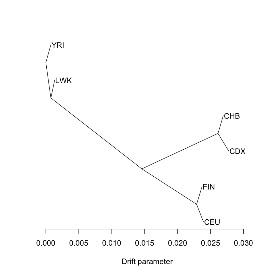
We selected data from six populations from the 1000 Genomes Project (see https:// www.internationalgenome.org/data-portal/data-collection/30x-grch38) that are supposedly not admixed: YRI (Yoruba in Ibadan, Nigeria; 108 individuals), LWK (Luhya in Webuye, Kenya; 99 individuals), CEU (Northern and Western European; 99 individuals), FIN (Finnish; 99 individuals), CHB (Han Chinese; 103 individuals), CDX (Dai Chinese; 93 individuals). The number of SNPs is 4,391,887; all SNPs with MAF >5%>5\%. Since the data set contains a large number of SNPs, we do not bias correct.

Using YRI as an outgroup, TreeMix produces the tree in fig. 6. In contrast, using either V^\widehat{V} or S^\widehat{S}, we identify the root to separate the clades (YRI, LWK) and (CEU, FIN, CHB, CDX), see fig. 7. Placing the root between the two clades would produce a more balanced, molecular clock-like tree.
Refer to caption
Figure 6: TreeMix tree of the six 1000 Genomes Project populations, forcing YRI to be the outgroup.
Refer to caption
Figure 7: Color-coding runs from dark red (small values) to dark blue (large values). Population 1: YRI, 2: CHB, 3: CDX, 4: LWK, 5: CEU, 6: FIN. For both statistics, the entries for pairs of populations in the two different clades, (YRI, LWK) and (CEU, FIN, CHB, CDX), are smaller than any other entry.

7 Proofs

7.1 Proof of theorem 2

Let AA be a symmetric m​×⁡mm\x m matrix. Let W=𝒲⁡(A)W=\sW(A). So

𝒟⁡(W)ij\displaystyle\sD(W)_{ij} =Wi​i+Wj​j−2​Wi​j\displaystyle=W_{ii}+W_{jj}-2W_{ij}
=Ai​i−2m​∑k=1mAi​k+1m2​∑k=1m∑ℓ=1mAk​ℓ\displaystyle=A_{ii}-\frac{2}{m}\sum_{k=1}^{m}A_{ik}+\frac{1}{m^{2}}\sum_{k=1}^{m}\sum_{\ell=1}^{m}A_{k\ell}
+Aj​j−2m​∑k=1mAj​k+1m2​∑k=1m∑ℓ=1mAk​ℓ\displaystyle\quad+A_{jj}-\frac{2}{m}\sum_{k=1}^{m}A_{jk}+\frac{1}{m^{2}}\sum_{k=1}^{m}\sum_{\ell=1}^{m}A_{k\ell}
−2​(Ai​j−1m​∑k=1mAi​k−1m​∑k=1mAj​k+1m2​∑k=1m∑ℓ=1mAk​ℓ)\displaystyle\quad-2\left(A_{ij}-\frac{1}{m}\sum_{k=1}^{m}A_{ik}-\frac{1}{m}\sum_{k=1}^{m}A_{jk}+\frac{1}{m^{2}}\sum_{k=1}^{m}\sum_{\ell=1}^{m}A_{k\ell}\right)
=Ai​i+Aj​j−2​Ai​j\displaystyle=A_{ii}+A_{jj}-2A_{ij}
=𝒟⁡(A)ij.\displaystyle=\sD(A)_{ij}.

It follows that 𝒟=𝒟∘𝒲\sD=\sD\circ\sW.

Let D=𝒟⁡(A)D=\sD(A). Then

−12​𝒲⁡(D)ij\displaystyle-\frac{1}{2}\sW(D)_{ij} =−12​Di​j+12​m​∑k=1mDi​k+12​m​∑k=1mDj​k−12​m2​∑k=1m∑ℓ=1mDk​ℓ\displaystyle=-\frac{1}{2}D_{ij}+\frac{1}{2m}\sum_{k=1}^{m}D_{ik}+\frac{1}{2m}\sum_{k=1}^{m}D_{jk}-\frac{1}{2m^{2}}\sum_{k=1}^{m}\sum_{\ell=1}^{m}D_{k\ell}
=−12​(Ai​i+Aj​j−2​Ai​j)+12​m​∑k=1m(Ai​i+Ak​k−2​Ai​k)\displaystyle=-\frac{1}{2}\left(A_{ii}+A_{jj}-2A_{ij}\right)+\frac{1}{2m}\sum_{k=1}^{m}\left(A_{ii}+A_{kk}-2A_{ik}\right)
+12​m∑k=1m(Aj​j+Ak​k−2Aj​k)−12​m2∑k=1m∑ℓ=1m(Ak​k+Aℓ​ℓ−2Ak​ℓ)\displaystyle\quad+\frac{1}{2m}\sum_{k=1}^{m}\left(A_{jj}+A_{kk}-2A_{jk}\right)-\frac{1}{2m^{2}}\sum_{k=1}^{m}\sum_{\ell=1}^{m}\left(A_{kk}+A_{\ell\ell}-2A_{k\ell}\right)
=Ai​j+12​m​∑k=1m(Ak​k−2​Ai​k)\displaystyle=A_{ij}+\frac{1}{2m}\sum_{k=1}^{m}\left(A_{kk}-2A_{ik}\right)
+12​m∑k=1m(Ak​k−2Aj​k)−12​m2∑k=1m∑ℓ=1m(Ak​k+Aℓ​ℓ−2Ak​ℓ)\displaystyle\quad+\frac{1}{2m}\sum_{k=1}^{m}\left(A_{kk}-2A_{jk}\right)-\frac{1}{2m^{2}}\sum_{k=1}^{m}\sum_{\ell=1}^{m}\left(A_{kk}+A_{\ell\ell}-2A_{k\ell}\right)
=Ai​j−1m​∑k=1mAi​k−1m​∑k=1mAj​k+1m2​∑k=1m∑ℓ=1mAk​ℓ\displaystyle=A_{ij}-\frac{1}{m}\sum_{k=1}^{m}A_{ik}-\frac{1}{m}\sum_{k=1}^{m}A_{jk}+\frac{1}{m^{2}}\sum_{k=1}^{m}\sum_{\ell=1}^{m}A_{k\ell}
=𝒲⁡(A)ij.\displaystyle=\sW(A)_{ij}.

It follows that −12𝒲∘𝒟=𝒲-\frac{1}{2}\sW\circ\sD=\sW.

Let D=𝒟⁡(A)D=\sD(A). Note that Di​i=Ai​i+Ai​i−2​Ai​i=0D_{ii}=A_{ii}+A_{ii}-2A_{ii}=0. It follows that 𝒟⁡(D)ij=Dii+Djj−2​Dij=−2​Dij\sD(D)_{ij}=D_{ii}+D_{jj}-2D_{ij}=-2D_{ij}, so 𝒟∘𝒟=−2𝒟\sD\circ\sD=-2\sD.

Note that

𝒲∘𝒲=\displaystyle\sW\circ\sW= (−12𝒲∘𝒟)∘𝒲=−12𝒲∘(𝒟∘𝒲)=−12𝒲∘𝒟=𝒲.\displaystyle(-\frac{1}{2}\sW\circ\sD)\circ\sW=-\frac{1}{2}\sW\circ(\sD\circ\sW)=-\frac{1}{2}\sW\circ\sD=\sW.

Let B∈im⁡(𝒟)B\in\im(\sD). Then, there is an A∈𝕊mA\in\mathbb{S}_{m} such that B=𝒟⁡(A)B=\sD(A). Hence,

−12𝒟(𝒲(B))=(𝒟∘−12𝒲∘𝒟)(A)=(𝒟∘𝒲)(A)=𝒟(A)=B.\displaystyle-\frac{1}{2}\sD(\sW(B))=(\sD\circ-\frac{1}{2}\sW\circ\sD)(A)=(\sD\circ\sW)(A)=\sD(A)=B.

Vice versa, let B∈im⁡(𝒲)B\in\im(\sW). Then, there is an A∈𝕊mA\in\mathbb{S}_{m} such that B=𝒲⁡(A)B=\sW(A). Hence,

𝒲(−12𝒟(B))=(−12𝒲∘𝒟∘𝒲)(A)=(𝒲∘𝒲)(A)=𝒲(A)=B.\displaystyle\sW(-\frac{1}{2}\sD(B))=(-\frac{1}{2}\sW\circ\sD\circ\sW)(A)=(\sW\circ\sW)(A)=\sW(A)=B.

It follows that

𝒲:im⁡(𝒟)→im⁡(𝒲)\sW:\im(\sD)\to\im(\sW)

is invertible with inverse

−12​𝒟:im⁡(𝒲)→im⁡(𝒟).-\frac{1}{2}\sD:\im(\sW)\to\im(\sD).

It follows from 𝒟=𝒟∘𝒲\sD=\sD\circ\sW that ker⁡(𝒲)⊆ker⁡(𝒟)\ker(\sW)\subseteq\ker(\sD) and it follows from 𝒲=−12𝒲∘𝒟\sW=-\frac{1}{2}\sW\circ\sD, that ker⁡(𝒟)⊆ker⁡(𝒲)\ker(\sD)\subseteq\ker(\sW). Hence ker⁡(𝒟)=ker⁡(𝒲)\ker(\sD)=\ker(\sW).

To calculate the kernel of 𝒲\sW and 𝒟\sD we make use of 𝒲\sW. Using eq. 3, 𝒲⁡(E)=(I−E/m)​E​(I−E/m)=(I−E/m)​(E−E)=0\sW(E)=(I-E/m)E(I-E/m)=(I-E/m)(E-E)=0, so E∈ker⁡(𝒲)E\in\ker(\sW). Note that E=e​(e/2)t+(e/2)​etE=e(e/2)^{t}+(e/2)e^{t}.

Let v∈ℝmv\in\R^{m} satisfy ∑i=1mvi=0\sum_{i=1}^{m}v_{i}=0. Then,

(I−E/m)​(e​vt+v​et)​(I−E/m)\displaystyle(I-E/m)(ev^{t}+ve^{t})(I-E/m) =(e​vt+v​et−e​vt−0)​(I−E/m)\displaystyle=(ev^{t}+ve^{t}-ev^{t}-0)(I-E/m)
=v​et​(I−E/m)=v​et−v​et=0.\displaystyle=ve^{t}(I-E/m)=ve^{t}-ve^{t}=0.

It follows that the kernel of 𝒲\sW contains {e​vt+v​et:v∈ℝm}\left\{ev^{t}+ve^{t}\colon v\in\R^{m}\right\}.

Now suppose AA is an arbitrary matrix in the kernel of 𝒲\sW. Then we might write A=λ​E+FA=\lambda E+F, where λ∈ℝ\lambda\in\R and FF is orthogonal to EE in the Frobenius inner product, from which follows that ∑i=1m∑j=1mFi​j=0\sum_{i=1}^{m}\sum_{j=1}^{m}F_{ij}=0, equivalent to E​F​E=0EFE=0. Moreover, 0=𝒲⁡(λ​E+F)=𝒲⁡(F)0=\sW(\lambda E+F)=\sW(F). It follows that

0\displaystyle 0 =(I−E/m)​F​(I−E/m)\displaystyle=(I-E/m)F(I-E/m)
=(F−E​F/m)​(I−E/m)\displaystyle=(F-EF/m)(I-E/m)
=F−E​F/m−F​E/m+E​F​E/(m2)\displaystyle=F-EF/m-FE/m+EFE/(m^{2})
=F−E​F/m−F​E/m.\displaystyle=F-EF/m-FE/m.

That is, F=E​F/m+F​E/mF=EF/m+FE/m. Note that

(E​F)i​j=\displaystyle(EF)_{ij}= ∑k=1mFk​j\displaystyle\sum_{k=1}^{m}F_{kj}

does not depend on ii. So there is a vector x∈ℝmx\in\R^{m}, so that

E​F=(xtxt).EF=\begin{pmatrix}x^{t}\\ \vdots\\ x^{t}\end{pmatrix}.

And we have F​E=(E​F)t=(x​…​x)FE=(EF)^{t}=(x\ldots x).

F=1m​(xtxt)+1m​(x​…​x)=e​xt/m+x​et/m.F=\frac{1}{m}\begin{pmatrix}x^{t}\\ \vdots\\ x^{t}\end{pmatrix}+\frac{1}{m}(x\ldots x)=ex^{t}/m+xe^{t}/m.

It follows that ker⁡(𝒲)={evt+vet:v∈ℝm}\ker(\sW)=\left\{ev^{t}+ve^{t}\colon v\in\R^{m}\right\}. The kernel has dimension mm. Since dim(𝕊m)=m⁡(m+1)/2\dim(\mathbb{S}_{m})=m(m+1)/2, it follows by the rank-nullity theorem that dim(im⁡(𝒲))=m⁡(m−1)/2\dim(\im(\sW))=m(m-1)/2.

It follows from (−12​𝒟)∘(−12​𝒟)=−12​𝒟(-\frac{1}{2}\sD)\circ(-\frac{1}{2}\sD)=-\frac{1}{2}\sD and 𝒲∘𝒲=𝒲\sW\circ\sW=\sW that −12​𝒟-\frac{1}{2}\sD and 𝒲\sW are projections.

Next we demonstrate that 𝒲\sW is an orthogonal projection by showing that the image space of 𝒲\sW is orthogonal to the kernel of 𝒲\sW. Let BB be a symmetric m​×⁡mm\x m-matrix. Then BB is orthogonal to the kernel if and only if for all v∈ℝmv\in\R^{m},

0=⟨B,e​vt+v​et⟩=∑i=1m∑j=1mBi​j​(vi+vj)=∑i=1mvi​∑j=1mBi​j+∑j=1mvj​∑i=1mBi​j=2​∑i=1mvi​∑j=1mBi​j.\begin{split}0&=\left\langle B,ev^{t}+ve^{t}\right\rangle=\sum_{i=1}^{m}\sum_{j=1}^{m}B_{ij}(v_{i}+v_{j})\\ &=\sum_{i=1}^{m}v_{i}\sum_{j=1}^{m}B_{ij}+\sum_{j=1}^{m}v_{j}\sum_{i=1}^{m}B_{ij}=2\sum_{i=1}^{m}v_{i}\sum_{j=1}^{m}B_{ij}.\end{split}

Note that {ei​et+e​eit:1≤i≤m}\left\{e_{i}e^{t}+ee_{i}^{t}:1\leq i\leq m\right\} is a basis for the kernel (where eie_{i} is the iith unit vector), and

⟨B,eiet+eeit⟩=2∑j=1mBi​j,i=1,…,m.\left\langle B,e_{i}e^{t}+ee_{i}^{t}\right\rangle=2\sum_{j=1}^{m}B_{ij},\quad i=1,\ldots,m.

Thus BB is orthogonal to ker⁡(𝒲)\ker(\sW) if and only if all rows of BB sum to zero.

Denote W=𝒲⁡(A)W=\sW(A). Note that

∑j=1mWi​j=\displaystyle\sum_{j=1}^{m}W_{ij}= ∑j=1mAi​j−∑k=1mAi​k−1m​∑j=1m∑k=1mAj​k+1m​∑k=1m∑ℓ=1mAk​ℓ=0,\displaystyle\sum_{j=1}^{m}A_{ij}-\sum_{k=1}^{m}A_{ik}-\frac{1}{m}\sum_{j=1}^{m}\sum_{k=1}^{m}A_{jk}+\frac{1}{m}\sum_{k=1}^{m}\sum_{\ell=1}^{m}A_{k\ell}=0,

for all i∈{1,…,m}i\in\left\{1,\ldots,m\right\}. It follows that 𝒲\sW is an orthogonal projection. Consequently, the operator norm is one.

From the fact that −12​𝒟-\frac{1}{2}\sD and 𝒲\sW have the same kernel, and im⁡(𝒲)≠im⁡(𝒟)\im(\sW)\not=\im(\sD) (elements of im⁡(𝒟)\im(\sD) has zero diagonal), it follows from unicity of orthogonal projections that −12​𝒟-\frac{1}{2}\sD cannot be an orthogonal projection.

Finally, let us calculate the operator norm of −12​𝒟-\frac{1}{2}\sD. We prove ‖−12​𝒟‖op=m\|-\frac{1}{2}\sD\|_{\text{op}}=\sqrt{m}, by showing that m\sqrt{m} is both a lower and an upper bound for ‖−12​𝒟‖op\|-\frac{1}{2}\sD\|_{\text{op}}.

First we prove that m\sqrt{m} is a lower bound of the operator norm. Note that −12​𝒟⁡(I−E/m)ij=−1-\frac{1}{2}\sD(I-E/m)_{ij}=-1 when i≠ji\neq j and zero otherwise. So ‖−12​𝒟⁡(I−E/m)‖F2=m⁡(m−1)\|-\frac{1}{2}\sD(I-E/m)\|_{F}^{2}=m(m-1). Note that ‖I−E/m‖F=m−1\|I-E/m\|_{F}=\sqrt{m-1}. So ‖−12​𝒟‖op≥‖−12​𝒟⁡(I−E/m)‖F‖I−E/m‖F=m⁡(m−1)m−1=m\|-\frac{1}{2}\sD\|_{\text{op}}\geq\frac{\|-\frac{1}{2}\sD(I-E/m)\|_{F}}{\|I-E/m\|_{F}}=\frac{\sqrt{m(m-1)}}{\sqrt{m-1}}=\sqrt{m}.

Let us continue with the upper bound. Let AA be an m​×⁡mm\x m-matrix of Frobenius norm one. We can write A=B+DA=B+D, where Bi​j=Ai​jB_{ij}=A_{ij} when i≠ji\neq j and Bi​i=0B_{ii}=0, and DD is a diagonal matrix with Di​i=Ai​iD_{ii}=A_{ii}, for all i,j=1,…,mi,j=1,\ldots,m. Note that BB and DD are orthogonal with respect to the Frobenius inner product. Then by the linearity of 𝒟\sD and the triangle inequality

‖−12​𝒟⁡(A)‖F≤‖−12​𝒟⁡(B)‖F+|12​𝒟⁡(D)|=‖B‖F+‖−12​𝒟⁡(D)‖F.\displaystyle\|-\frac{1}{2}\sD(A)\|_{F}\leq\|-\frac{1}{2}\sD(B)\|_{F}+\|\frac{1}{2}\sD(D)\|=\|B\|_{F}+\|-\frac{1}{2}\sD(D)\|_{F}.

We can write

D=∑i=1mAi​i​ei​eiT.D=\sum_{i=1}^{m}A_{ii}e_{i}e_{i}^{T}.

Note that {eiejT:i,j∈{1,…,m}}\left\{e_{i}e_{j}^{T}:i,j\in\left\{1,\ldots,m\right\}\right\} is an orthonormal basis of the space of m​×⁡mm\x m-matrices in the Frobenius inner product. We have

−12​𝒟⁡(ek​ekT)=ek​ekT−12​eekT−12​ek​eT.\displaystyle-\frac{1}{2}\sD(e_{k}e_{k}^{T})=e_{k}e_{k}^{T}-\frac{1}{2}ee_{k}^{T}-\frac{1}{2}e_{k}e^{T}.

So

⟨−12​𝒟⁡(ea​eaT),−12​𝒟⁡(eb​ebT)⟩=\displaystyle\left\langle-\frac{1}{2}\sD(e_{a}e_{a}^{T}),-\frac{1}{2}\sD(e_{b}e_{b}^{T})\right\rangle= {12 if ​a≠b,12​(m−1) if ​a=b.\displaystyle\begin{cases}\frac{1}{2}&\text{ if }a\neq b,\\ \frac{1}{2}(m-1)&\text{ if }a=b.\end{cases}

We have

−12𝒟(D)=−12𝒟(∑i=1mAiieieiT)=−12∑i=1mAii𝒟(eieiT)\displaystyle-\frac{1}{2}\sD(D)=-\frac{1}{2}\sD\left(\sum_{i=1}^{m}A_{ii}e_{i}e_{i}^{T}\right)=-\frac{1}{2}\sum_{i=1}^{m}A_{ii}\sD\left(e_{i}e_{i}^{T}\right)

So

‖−12𝒟(D)‖F2=⟨−12∑i=1mAi​i𝒟(eieiT),−12∑i=1mAii𝒟(eieiT)⟩\displaystyle\left\|-\frac{1}{2}\sD(D)\right\|_{F}^{2}=\left\langle-\frac{1}{2}\sum_{i=1}^{m}A_{ii}\sD\left(e_{i}e_{i}^{T}\right),-\frac{1}{2}\sum_{i=1}^{m}A_{ii}\sD\left(e_{i}e_{i}^{T}\right)\right\rangle
=\displaystyle= 12∑i,j:i≠jAi​iAj​j+12(m−1)∑i=1mAi​i2.\displaystyle\frac{1}{2}\sum_{i,j:i\neq j}A_{ii}A_{jj}+\frac{1}{2}(m-1)\sum_{i=1}^{m}A_{ii}^{2}.

Using that Ai​i​Aj​j≤12​Ai​i2+12​Aj​j2A_{ii}A_{jj}\leq\frac{1}{2}A_{ii}^{2}+\frac{1}{2}A_{jj}^{2}, we see that

‖−12​𝒟⁡(D)‖F2≤\displaystyle\left\|-\frac{1}{2}\sD(D)\right\|_{F}^{2}\leq 14∑i,j:i≠j(Ai​i2+Aj​j2)+12(m−1)∑i=1mAi​i2\displaystyle\frac{1}{4}\sum_{i,j:i\neq j}(A_{ii}^{2}+A_{jj}^{2})+\frac{1}{2}(m-1)\sum_{i=1}^{m}A_{ii}^{2}
=\displaystyle= 14​∑i=1m∑j=1m(Ai​i2+Aj​j2)+12​(m−2)​∑i=1mAi​i2\displaystyle\frac{1}{4}\sum_{i=1}^{m}\sum_{j=1}^{m}(A_{ii}^{2}+A_{jj}^{2})+\frac{1}{2}(m-2)\sum_{i=1}^{m}A_{ii}^{2}
=\displaystyle= (m−1)​∑i=1mAi​i2\displaystyle(m-1)\sum_{i=1}^{m}A_{ii}^{2}
=\displaystyle= (m−1)​‖D‖F2.\displaystyle(m-1)\|D\|_{F}^{2}.

As ‖A‖F=1\|A\|_{F}=1, and BB and DD are orthogonal, we have 1=‖B‖F2+‖D‖F21=\|B\|_{F}^{2}+\|D\|_{F}^{2}. Let α=‖D‖F2∈[0,1]\alpha=\|D\|_{F}^{2}\in[0,1], then ‖B‖F2=1−α\|B\|_{F}^{2}=1-\alpha. So

‖−12​𝒟⁡(A)‖F≤1−α+(m−1)​α=:f⁡(α).\displaystyle\|-\frac{1}{2}\sD(A)\|_{F}\leq\sqrt{1-\alpha}+\sqrt{(m-1)\alpha}=:f(\alpha).

With simple algebra one can show that the maximum of ff is attained for α=m−1m\alpha=\frac{m-1}{m}. So

‖−12​𝒟⁡(A)‖F≤\displaystyle\|-\frac{1}{2}\sD(A)\|_{F}\leq 1m+(m−1)2m=m.\displaystyle\sqrt{\frac{1}{m}}+\sqrt{\frac{(m-1)^{2}}{m}}=\sqrt{m}.

It follows that both the upper and lower bound of ‖−12​𝒟‖op\|-\frac{1}{2}\sD\|_{\text{op}} are m\sqrt{m}, so ‖−12​𝒟‖op=m\|-\frac{1}{2}\sD\|_{\text{op}}=\sqrt{m}.

7.2 Proof of theorem 7

Define V^k=Xk​(Xk)t−μ^k2​E\widehat{V}^{k}=X^{k}(X^{k})^{t}-\hat{\mu}_{k}^{2}E with entries V^a​bk\widehat{V}^{k}_{ab}, a,b=1,…,ma,b=1,\ldots,m, then V^=1n​∑k=1nV^k\widehat{V}=\frac{1}{n}\sum_{k=1}^{n}\widehat{V}^{k}.

Trivially for x1,x2,x3,x4∈ℝx_{1},x_{2},x_{3},x_{4}\in\mathbb{R}, |x1​x2​x3​x4|≤x14+x24+x34+x44|x_{1}x_{2}x_{3}x_{4}|\leq x_{1}^{4}+x_{2}^{4}+x_{3}^{4}+x_{4}^{4}. So we have for

V^a​bk\displaystyle\widehat{V}^{k}_{ab} =Xak​Xbk−1m2​∑c=1m∑d=1mXck​Xdk\displaystyle=X_{a}^{k}X_{b}^{k}-\frac{1}{m^{2}}\sum_{c=1}^{m}\sum_{d=1}^{m}X_{c}^{k}X_{d}^{k}
that
𝔼⁡((V^abk)2)\displaystyle\E((\widehat{V}_{ab}^{k})^{2}) ≤E⁡((Xak)2​(Xbk)2)+1m4​(∑c=1m∑d=1mXck​Xdk)2+2m2​𝔼⁡(Xak​Xbk​∑c=1m∑d=1mXck​Xdk)\displaystyle\leq E((X_{a}^{k})^{2}(X_{b}^{k})^{2})+\frac{1}{m^{4}}\left(\sum_{c=1}^{m}\sum_{d=1}^{m}X_{c}^{k}X_{d}^{k}\right)^{\!\!2}+\frac{2}{m^{2}}\E\left(X_{a}^{k}X_{b}^{k}\sum_{c=1}^{m}\sum_{d=1}^{m}X_{c}^{k}X_{d}^{k}\right)
≤4​C+4​C+8​C=16​C,\displaystyle\leq 4C+4C+8C=16C,

where it is assumed that all moments of XakX_{a}^{k} up to order four are bounded uniformly in k=1,…,nk=1,\ldots,n and a=1,…,ma=1,\ldots,m, by some number C>0C>0. Hence,

var⁡(V^a​bk)\displaystyle\var(\widehat{V}^{k}_{ab}) ≤𝔼⁡((V^abk)2)≤16​C.\displaystyle\leq\E((\widehat{V}_{ab}^{k})^{2})\leq 16C.

As V^k,V^k+t,…,Vk+⌊(n−k)/t⌋​t\widehat{V}^{k},\widehat{V}^{k+t},\ldots,V^{k+\left\lfloor(n-k)/t\right\rfloor t} are independent, for k=1,…,tk=1,\ldots,t, we have

var⁡(1n​(V^a​bk+V^(k+t)​a​b+…+V(k+⌊(n−k)/t⌋​t)​a​b))\displaystyle\var\left(\frac{1}{n}\left(\widehat{V}^{k}_{ab}+\widehat{V}_{(k+t)ab}+\ldots+V_{(k+\left\lfloor(n-k)/t\right\rfloor t)ab}\right)\right) ≤⌊(n−k)/t⌋n2​16​C≤16n​t​C.\displaystyle\leq\frac{\left\lfloor(n-k)/t\right\rfloor}{n^{2}}16C\leq\frac{16}{nt}C.

Applying corollary 15 gives

var⁡(V^a​b)\displaystyle\var(\widehat{V}_{ab}) ≤16​t2n​t​C=16​tn​C.\displaystyle\leq\frac{16t^{2}}{nt}C=\frac{16t}{n}C.

It follows that

𝔼⁡[‖V^−V‖F2]\displaystyle\E[\|\widehat{V}-V\|_{F}^{2}] =∑a=1m∑b=1mvar⁡(V^a​b)≤16​m2​tn​C.\displaystyle=\sum_{a=1}^{m}\sum_{b=1}^{m}\var(\widehat{V}_{ab})\leq\frac{16m^{2}t}{n}C.

Consequently, by Jensen’s inequality the claim follows: 𝔼⁡(‖V^−V‖F)2≤𝔼⁡(‖V^−V‖F2)\E(\|\widehat{V}-V\|_{F})^{2}\leq\E(\|\widehat{V}-V\|_{F}^{2}).

It follows from theorem 6 in combination with the definition of 𝒟\sD, that D^i​j=V^i​i+V^j​j−2​V^i​j\widehat{D}_{ij}=\widehat{V}_{ii}+\widehat{V}_{jj}-2\widehat{V}_{ij}. Similarly, using corollary 15 again and the definition of 𝒟\sD, gives var⁡(D^i​j)≤256​tn​C\var(\widehat{D}_{ij})\leq\frac{256t}{n}C. Using 𝔼⁡(D^)=D\E(\widehat{D})=D, the claim for 𝔼⁡(‖D^−D‖F)\E(\|\widehat{D}-D\|_{F}) follows similarly to that for V^\widehat{V}.

Finally, from theorem 6,

W^i​j=V^i​j−1m​∑a=1mV^i​a−1m​∑a=1mV^j​a+1m2​∑a=1m∑b=1mV^a​b.\widehat{W}_{ij}=\widehat{V}_{ij}-\frac{1}{m}\sum_{a=1}^{m}\widehat{V}_{ia}-\frac{1}{m}\sum_{a=1}^{m}\widehat{V}_{ja}+\frac{1}{m^{2}}\sum_{a=1}^{m}\sum_{b=1}^{m}\widehat{V}_{ab}.

Applying corollary 15 gives

var⁡(W^i​j)\displaystyle\var(\widehat{W}_{ij}) ≤4​(var⁡(V^i​j)+var⁡(1m​∑a=1mV^i​a)+var⁡(1m​∑a=1mV^j​a)+var⁡(1m2​∑a=1m∑b=1mV^a​b))\displaystyle\leq 4\left(\var(\widehat{V}_{ij})+\var\left(\frac{1}{m}\sum_{a=1}^{m}\widehat{V}_{ia}\right)+\var\left(\frac{1}{m}\sum_{a=1}^{m}\widehat{V}_{ja}\right)+\var\left(\frac{1}{m^{2}}\sum_{a=1}^{m}\sum_{b=1}^{m}\widehat{V}_{ab}\right)\right)
≤256​tn​C.\displaystyle\leq\frac{256t}{n}C.

Again, in a similar way to that of V^\widehat{V}, the claim for 𝔼⁡(‖W^−W‖F)\E(\|\widehat{W}-W\|_{F}) follows.

7.3 Proof of theorem 12

Define S^k=(X2​k−X2​k−1)​(X2​k−X2​k−1)t\hat{S}^{k}=(X^{2k}-X^{2k-1})(X^{2k}-X^{2k-1})^{t}. Then we have

var⁡(S^a​bK)≤\displaystyle\var(\hat{S}_{ab}^{K})\leq 𝔼⁡[(Xa2​k−Xa2​k−1)2​(Xb2​k−Xb2​k−1)2]\displaystyle\E\left[\left(X^{2k}_{a}-X^{2k-1}_{a}\right)^{2}\left(X^{2k}_{b}-X^{2k-1}_{b}\right)^{2}\right]
=\displaystyle= 𝔼⁡[(Xa2​k​Xb2​k−Xa2​k​Xb2​k−1−Xa2​k−1​Xb2​k+Xa2​k−1​Xb2​k−1)2].\displaystyle\E\left[\left(X_{a}^{2k}X_{b}^{2k}-X_{a}^{2k}X_{b}^{2k-1}-X_{a}^{2k-1}X_{b}^{2k}+X_{a}^{2k-1}X_{b}^{2k-1}\right)^{2}\right].

The latter can be written as a sum of 16 elements 𝔼⁡[Xac​Xad​Xbe​Xbf]\E\left[X_{a}^{c}X_{a}^{d}X_{b}^{e}X_{b}^{f}\right], where c,d,e,f∈{2​k−1,2​k}c,d,e,f\in\left\{2k-1,2k\right\}. Applying the Jensen’s inequality and then Hölder’s inequality twice gives

|𝔼⁡[Xac​Xad​Xbe​Xbf]|\displaystyle\left|\E\left[X_{a}^{c}X_{a}^{d}X_{b}^{e}X_{b}^{f}\right]\right| ≤𝔼⁡[|Xac​Xad​Xbe​Xbf|]\displaystyle\leq\E\left[\left|X_{a}^{c}X_{a}^{d}X_{b}^{e}X_{b}^{f}\right|\right]
≤𝔼⁡[(Xac)2​(Xad)2]​𝔼⁡[(Xbe)2​(Xbf)2]\displaystyle\leq\sqrt{\E\left[(X_{a}^{c})^{2}(X_{a}^{d})^{2}\right]\E\left[(X_{b}^{e})^{2}(X_{b}^{f})^{2}\right]}
≤𝔼⁡[(Xac)4]​𝔼​[(Xad)4]​𝔼​[(Xbe)4]​𝔼​[(Xbf)4]4\displaystyle\leq\sqrt[4]{\E\left[(X_{a}^{c})^{4}\right]\E\left[(X_{a}^{d})^{4}\right]\E\left[(X_{b}^{e})^{4}\right]\E\left[(X_{b}^{f})^{4}\right]}
≤C44=C.\displaystyle\leq\sqrt[4]{C^{4}}=C.

It follows that var⁡(S^a​bK)≤16​C\var(\hat{S}_{ab}^{K})\leq 16C.

So S^=1⌊n/2⌋​∑k=1⌊n/2⌋S^k\hat{S}=\frac{1}{\left\lfloor n/2\right\rfloor}\sum_{k=1}^{\left\lfloor n/2\right\rfloor}\hat{S}^{k}. As S^k,\hat{S}^{k}, S^k+t,\hat{S}_{k+t}, …,S^k+⌊(⌊n/2⌋−k)/t⌋​t\ldots,\hat{S}_{k+\left\lfloor(\left\lfloor n/2\right\rfloor-k)/t\right\rfloor t} are independent, for k=1,…,tk=1,\ldots,t, we have

var⁡(1⌊n/2⌋​(S^a​bk+S^a​bk+t+…+S^a​bk+⌊(⌊n/2⌋−k)/t⌋​t))\displaystyle\var\left(\frac{1}{\left\lfloor n/2\right\rfloor}\left(\hat{S}_{ab}^{k}+\hat{S}_{ab}^{k+t}+\ldots+\hat{S}_{ab}^{k+\left\lfloor(\left\lfloor n/2\right\rfloor-k)/t\right\rfloor t}\right)\right)
≤⌊(⌊n/2⌋−k)/t⌋⌊n/2⌋2​16​C≤16​C⌊n/2⌋​t.\displaystyle\leq\frac{\left\lfloor(\left\lfloor n/2\right\rfloor-k)/t\right\rfloor}{\left\lfloor n/2\right\rfloor^{2}}16C\leq\frac{16C}{\left\lfloor n/2\right\rfloor t}.

Applying corollary 15 gives

var⁡(S^a​b)\displaystyle\var(\hat{S}_{ab}) =var⁡(∑k=1t1⌊n/2⌋​(S^a​bk+S^a​bk+t+…+S^a​bk+⌊(⌊n/2⌋−k)/t⌋​t))\displaystyle=\var\left(\sum_{k=1}^{t}\frac{1}{\left\lfloor n/2\right\rfloor}\left(\hat{S}_{ab}^{k}+\hat{S}_{ab}^{k+t}+\ldots+\hat{S}_{ab}^{k+\left\lfloor(\left\lfloor n/2\right\rfloor-k)/t\right\rfloor t}\right)\right)
≤t∑k=1tvar(1⌊n/2⌋(S^a​bk+S^a​bk+t+…+S^a​b(k+⌊⌊n/2⌋−k)/t⌋t))\displaystyle\leq t\sum_{k=1}^{t}\var\left(\frac{1}{\left\lfloor n/2\right\rfloor}\left(\hat{S}_{ab}^{k}+\hat{S}_{ab}^{k+t}+\ldots+\hat{S}_{ab}^{(k+\left\lfloor\left\lfloor n/2\right\rfloor-k)/t\right\rfloor t}\right)\right)
≤t​∑k=1t16​C⌊n/2⌋​t\displaystyle\leq t\sum_{k=1}^{t}\frac{16C}{\left\lfloor n/2\right\rfloor t}
=16​C⌊n/2⌋​t.\displaystyle=\frac{16C}{\left\lfloor n/2\right\rfloor}t.

It follows that

𝔼⁡[‖S^−Σ1‖22]=\displaystyle\E[\|\hat{S}-\Sigma_{1}\|_{2}^{2}]= ∑a=1m∑b=1mvar⁡(Σ~a​b)≤16​m2​t⌊n/2⌋​C,\displaystyle\sum_{a=1}^{m}\sum_{b=1}^{m}\var(\widetilde{\Sigma}_{ab})\leq\frac{16m^{2}t}{\left\lfloor n/2\right\rfloor}C,

and by Jensen’s inequality that

𝔼⁡[‖S^−Σ1‖2]≤𝔼⁡[‖S^−Σ1‖22]≤4​m2​t⌊n/2⌋​C.\E[\|\hat{S}-\Sigma_{1}\|_{2}]\leq\sqrt{\E[\|\hat{S}-\Sigma_{1}\|_{2}^{2}]}\leq 4\sqrt{\frac{m^{2}t}{\left\lfloor n/2\right\rfloor}C}.

8 Auxiliary results

Lemma 13.

Let x,y∈ℝx,y\in\R. Then |x​y|≤12​(x2+y2)|xy|\leq\frac{1}{2}(x^{2}+y^{2}).

Proof.

It follows from 0≤(x−y)2=x2+y2−2​x​y0\leq(x-y)^{2}=x^{2}+y^{2}-2xy and 0≤(x+y)2=x2+y2+2​x​y0\leq(x+y)^{2}=x^{2}+y^{2}+2xy that |2​x​y|≤x2+y2|2xy|\leq x^{2}+y^{2}. ∎

Lemma 14.

Let x1,…,xm∈ℝx_{1},\ldots,x_{m}\in\R. Then (∑i=1mxi)2≤m​∑i=1mxi2(\sum_{i=1}^{m}x_{i})^{2}\leq m\sum_{i=1}^{m}x_{i}^{2}.

Proof.

From lemma 13, (∑i=1mxi)2=∑i=1m∑j=1mxi​xj≤12​∑i=1m∑j=1m(xi2+xj2)=m​∑i=1mxi2(\sum_{i=1}^{m}x_{i})^{2}=\sum_{i=1}^{m}\sum_{j=1}^{m}x_{i}x_{j}\leq\frac{1}{2}\sum_{i=1}^{m}\sum_{j=1}^{m}(x_{i}^{2}+x_{j}^{2})=m\sum_{i=1}^{m}x_{i}^{2}. ∎

Corollary 15.

Let X1,…,XmX_{1},\ldots,X_{m} be random variables. Then, Var​(∑k=1mXk)\textrm{Var}(\sum_{k=1}^{m}X_{k}) ≤m​∑k=1mVar​(Xk)\leq m\sum_{k=1}^{m}\textrm{Var}(X_{k}).

Proof.

Take xk=Xk−𝔼⁡[Xk]x_{k}=X_{k}-\E[X_{k}] and expectation in lemma 14. ∎

Acknowledgements

CW and JvW are supported by the Independent Research Fund Denmark (grant number: 8021-00360B) and the University of Copenhagen through the Data+ initiative. ZI is supported by the Novo Nordisk Foundation, Denmark (grant number: NNF20OC0061343).

References

  • DeGiorgio et al. (2009) DeGiorgio, M., M. Jakobsson, and N. A. Rosenberg (2009): “Out of Africa: modern humanorigins special feature: explaining worldwide patterns of human genetic variation using a coalescent-based serial founder model of migration outward from africa,” Proc. Natl. Acad. Sci. U S A, 106, 16057–62.
  • Escalona et al. (2016) Escalona, M., S. Rocha, and D. Posada (2016): “A comparison of tools for the simulation of genomic next-generation sequencing data,” Nat. Rev. Genet., 17, 459–69.
  • Hakemi (1962) Hakemi, S. L. (1962): “On realizability of a set of integers as degrees of the vertices of a linear graph. i,” Journal of the Society for Industrial and Applied Mathematics, 10, 496–506.
  • Hudson (1983) Hudson, R. R. (1983): “Properties of a neutral allele model with intragenic recombinationl,” Theoretical Population Biology, 23, 183–201.
  • Hudson (2002) Hudson, R. R. (2002): “Generating samples under a wright-fisher neutral model of genetic variation,” Bioinformatics, 18, 337–338.
  • Korunes and Goldberg (2021) Korunes, K. L. and A. Goldberg (2021): “Human genetic admixture,” PLoS Genet., 17, e1009374.
  • Leppala et al. (2017) Leppala, K., S. Nielsen, and T. Mailund (2017): “admixturegraph: an r package for admixture graph manipulation and fitting,” Bioinformatics, 33, 1738–40.
  • Lipson (2020) Lipson, M. (2020): “Applying f4f_{4}-statistics and admixture graphs: Theory and examples,” Mol. Ecol. Res., 20, 1658–67.
  • Nicholson et al. (2002) Nicholson, G., A. V. Smith, F. Jonsson, O. Gustafsson, K. Stefansson, and P. Donnelly (2002): “Assessing population differentiation and isolation from single-nucleotide polymorphism data,” J.R. Statist. Soc. B, 64, 695–715.
  • Patterson et al. (2012) Patterson, N., P. Moorjani, Y. Luo, S. Mallick, N. Rohland, Y. Zhan, T. Genschoreck, T. Webster, and D. Reich (2012): “Ancient admixture in human history,” Genetics, 192, 1065–1093.
  • Pickrell and Pritchard (2012) Pickrell, J. and J. Pritchard (2012): “Inference of population splits and mixtures from genome-wide allele frequency data,” PLOS Genetics, 8, 1–17.
  • (12) Semple, C. and M. Steel (????): Phylogenetics, Oxford lecture series in mathematics and its applications, Oxford University Press.