跳到论文正文
W Papers独立论文阅读器 arXiv:2201.09040 论文正文 计算阅读时间 · 0%
引用这篇论文根据当前论文元数据生成,正式投稿前建议核对。


License: CC BY 4.0
arXiv:2201.09040v1 [math.ST] 22 Jan 2022

Optimal Estimation and Computational Limit of Low-rank Gaussian Mixtures

Zhongyuan Lyu    Dong Xia Note: Dong Xia’s research was partially supported by Hong Kong RGC Grant ECS 26302019, GRF 16303320 and GRF 16300121. Affiliation:  Hong Kong University of Science and Technology
(August 11, 2026)
Abstract

Structural matrix-variate observations routinely arise in diverse fields such as multi-layer network analysis and brain image clustering. While data of this type have been extensively investigated with fruitful outcomes being delivered, the fundamental questions like its statistical optimality and computational limit are largely under-explored. In this paper, we propose a low-rank Gaussian mixture model (LrMM) assuming each matrix-valued observation has a planted low-rank structure. Minimax lower bounds for estimating the underlying low-rank matrix are established allowing a whole range of sample sizes and signal strength. Under a minimal condition on signal strength, referred to as the information-theoretical limit or statistical limit, we prove the minimax optimality of a maximum likelihood estimator which, in general, is computationally infeasible. If the signal is stronger than a certain threshold, called the computational limit, we design a computationally fast estimator based on spectral aggregation and demonstrate its minimax optimality. Moreover, when the signal strength is smaller than the computational limit, we provide evidences based on the low-degree likelihood ratio framework to claim that no polynomial-time algorithm can consistently recover the underlying low-rank matrix. Our results reveal multiple phase transitions in the minimax error rates and the statistical-to-computational gap. Numerical experiments confirm our theoretical findings. We further showcase the merit of our spectral aggregation method on the worldwide food trading dataset.

1 Introduction

The recent decade has witnessed a burgeoning demand in processing and analyzing large-scale matrix-variate data which routinely arise in diverse fields. In gene expression analysis, e.g., the BHL (brain, heart and lung) dataset (BHL; Mai et al. 2021), the measurement of gene expression on different types of tissues is often repeated for multiple times. The resultant observation for each tissue becomes a matrix and thus the cluster analysis is operated on matrix-valued observations. A multi-layer network (Le et al. 2018; Jing et al. 2021; Lyu et al. 2021; Paul and Chen 2020) usually consists of multiple networks on the same set of vertices. Since each observed layer is equivalently represented as an adjacent matrix, problems such as community detection (Paul and Chen 2020), layer clustering (Jing et al. 2021) and common probability matrix estimation (Le et al. 2018) are generally attacked by statistical analysis on a collection of adjacency matrices. Other notable examples include brain image clustering (Sun and Li 2019; Wang et al. 2017), EEG data analysis (Hu et al. 2020; Gao et al. 2021), etc. Oftentimes, the dimensions of observed matrices are ultra-large or the number of matrix-valued observations is relatively small, which has motivated the exploration of hidden low-dimensional structures, e.g. sparsity and low-rankness, in matrix-valued observations. All the aforementioned works assumed, among others, certain types of low-rank structures for the underlying parameters of interest and have delivered fruitful outcomes in real-world applications.

Inspired by those foregoing works, throughout this paper, we assume that each matrix-valued observation has a low-rank expectation which might vary for different observations. Towards that end, several specific low-rank statistical models, tailored for concrete applications, and respective estimating procedures have been proposed. For instance, a mixture multi-layer stochastic block model (SBM) was introduced in Jing et al. 2021 for uncovering the global and local communities in multi-layer networks. At the core of this model is the assumption that every layer has a low-rank expected adjacency matrix. Their estimator was based on the (regularized) low-rank tensor decomposition. A special multi-layer SBM was proposed by Paul and Chen 2020 and estimated by a spectral method. In order to analyze the brain fMRI data, Sun and Li 2019 proposed a tensor Gaussian mixture model and designed an estimator via (fusedly-)truncated low-rank tensor decomposition. Despite these prior efforts, usually motivated by particular applications, on the low-rank estimates from a mixture of matrix-valued observations, many fundamental questions remain unanswered. What is the role and benefit of low-rankness? How do the sample size and signal strength (see the definition after eq.(2)) characterize the intrinsic difficulty, i.e., are there any phase transitions? What is the statistically optimal rate, which estimator can achieve the rate and is this estimator computationally feasible? What is the fastest error rate achievable by estimators requiring only polynomial-time complexity? This paper aims to answer all these questions and provides a complete picture for the statistical and computational limits in the low-rank estimation from a mixture of matrix-valued observations.

We now introduce the low-rank Gaussian mixture model (LrMM) to formalize the questions. For simplicity, we focus on the mixture of two components and will briefly discuss the case of multiple components in Section 7. The d1×d2d_{1}\times d_{2} matrix 𝐗\mathbf{X} is said to follow an isotropic matrix normal (Gupta and Nagar 2018) distribution 𝒩⁡(𝐌,𝐈d1⊗𝐈d2){\cal N}(\mathbf{M},\mathbf{I}_{d_{1}}\otimes\mathbf{I}_{d_{2}}) if 𝑣𝑒𝑐⁡(𝐗)∼𝒩⁡(𝑣𝑒𝑐⁡(𝐌),𝐈d1​d2){\it vec}(\mathbf{X})\sim{\cal N}\big({\it vec}(\mathbf{M}),\mathbf{I}_{d_{1}d_{2}}\big), where 𝐈d\mathbf{I}_{d} represents the d×dd\times d identity matrix and 𝐌\mathbf{M} is a deterministic matrix. Clearly, this implies that 𝐗\mathbf{X} is equal to 𝐌+𝐙\mathbf{M}+\mathbf{Z} in distribution where 𝐙\mathbf{Z} has i.i.d. standard normal entries. Denote11 1 With a slight abuse of notation, we also denote p𝐌p_{\mathbf{M}} the associated probability density function.

p𝐌=12​𝒩​(𝐌,𝐈d1⊗𝐈d2)+12​𝒩​(−𝐌,𝐈d1⊗𝐈d2)p_{\mathbf{M}}=\frac{1}{2}{\cal N}(\mathbf{M},\mathbf{I}_{d_{1}}\otimes\mathbf{I}_{d_{2}})+\frac{1}{2}{\cal N}(-\mathbf{M},\mathbf{I}_{d_{1}}\otimes\mathbf{I}_{d_{2}}) (1)

the symmetric mixture of two-component Gaussian mixture model. Then 𝐗∼p𝐌\mathbf{X}\sim p_{\mathbf{M}} means that 𝐗\mathbf{X} is sampled from 𝒩⁡(𝐌,𝐈d1⊗𝐈d2){\cal N}(\mathbf{M},\mathbf{I}_{d_{1}}\otimes\mathbf{I}_{d_{2}}) and 𝒩⁡(−𝐌,𝐈d1⊗𝐈d2){\cal N}(-\mathbf{M},\mathbf{I}_{d_{1}}\otimes\mathbf{I}_{d_{2}}) with probability both 1/21/2, respectively. Put it differently, 𝐗\mathbf{X} equals s​𝐌+𝐙s\mathbf{M}+\mathbf{Z} in distribution with ss being a Rademacher random variable, called the label of 𝐗\mathbf{X}, satisfying ℙ⁡(s=±1)=1/2\mathbb{P}(s=\pm 1)=1/2. Throughout the paper, we assume that 𝐌\mathbf{M} has a small rank, i.e., r=rank⁡(𝐌)≪min⁡{d1,d2}r={\rm rank}(\mathbf{M})\ll\min\{d_{1},d_{2}\}. Note that, under model (1), the marginal expectation of 𝐗\mathbf{X} is actually zero. The former claim of low-rank expectation in the last paragraph actually refers to the conditional expectation 𝔼⁡(𝐗|s)=s​𝐌\mathbb{E}(\mathbf{X}|s)=s\mathbf{M} which is low-rank. We remark that the condition of equal prior probabilities is not essential and can be slightly relaxed. The assumption of symmetry of the two components is only for ease of exposition. If the two components have distinct mean matrices, say 𝐌1\mathbf{M}_{1} and 𝐌2\mathbf{M}_{2}, respectively, one can first estimate the average (𝐌1+𝐌2)/2(\mathbf{M}_{1}+\mathbf{M}_{2})/2, subtract it from all observations and reduce the problem to the symmetric case. Similarly, the assumption of isotropic noise is relaxable as long as the covariance tensor is known. The case of unknown covariance is much more challenging (Davis et al. 2021; Bakshi et al. 2020; Belkin and Sinha 2010; Cai et al. 2019; Ge et al. 2015; Moitra and Valiant 2010) even in the vector case and is beyond the scope of the current paper.

Given i.i.d. observations 𝐗,𝐗1,⋯,𝐗n\mathbf{X},\mathbf{X}_{1},\cdots,\mathbf{X}_{n} sampled from the mixture distribution p𝐌p_{\mathbf{M}} in (1), our goals are to estimate the latent low-rank matrix 𝐌\mathbf{M}, establish the minimax error rates and design computationally efficient estimators. We assume d1≍d2≍dd_{1}\asymp d_{2}\asymp d meaning that there exist absolute constants c0,C0>0c_{0},C_{0}>0 satisfying c0​d≤min⁡{d1,d2}≤max⁡{d1,d2}≤C0​dc_{0}d\leq\min\{d_{1},d_{2}\}\leq\max\{d_{1},d_{2}\}\leq C_{0}d. The parameter space of interest is, for any λ>0\lambda>0,

ℳd1,d2(r,λ):={𝐌∈ℝd1×d2:rank(𝐌)=r,λ≍σr(𝐌)≤⋯≤σ1(𝐌)≍λ}{\cal M}_{d_{1},d_{2}}(r,\lambda):=\left\{\mathbf{M}\in\mathbb{R}^{d_{1}\times d_{2}}:{\rm rank}(\mathbf{M})=r,\ \lambda\asymp\sigma_{r}(\mathbf{M})\leq\cdots\leq\sigma_{1}(\mathbf{M})\asymp\lambda\right\} (2)

where σk​(⋅)\sigma_{k}(\cdot) denotes the kk-th largest singular value of a matrix. For notational brevity, we shall write ℳ⁡(r,λ){\cal M}(r,\lambda) for short. The signal strength of low-rank models is usually determined by the smallest non-zero singular value (Koltchinskii and Xia 2016; Zhang and Xia 2018; Xia 2021; Cheng et al. 2021; Gavish and Donoho 2014). The set ℳd1,d2​(r,λ){\cal M}_{d_{1},d_{2}}(r,\lambda) is the collection of all d1×d2d_{1}\times d_{2} rank-rr matrices whose signal strength is of order λ\lambda. For simplicity, we only focus on the well-conditioned matrices, i.e., with a bounded condition number. The minimax error rate of estimating 𝐌\mathbf{M} is defined by inf^​𝐌sup𝐌∈ℳ⁡(r,λ)𝔼​ℓ​(^​𝐌,𝐌)\inf_{\widehat{}\mathbf{M}}\sup_{\mathbf{M}\in{\cal M}(r,\lambda)}\mathbb{E}\ell(\widehat{}\mathbf{M},\mathbf{M}) , where the infimum is taken over all possible estimator ^​𝐌\widehat{}\mathbf{M} constructed from the i.i.d. observations 𝐗1,⋯,𝐗n\mathbf{X}_{1},\cdots,\mathbf{X}_{n} and the loss function is ℓ⁡(^​𝐌,𝐌):=minη=±1⁡‖^​𝐌−η​𝐌‖F\ell(\widehat{}\mathbf{M},\mathbf{M}):=\min_{\eta=\pm 1}\|\widehat{}\mathbf{M}-\eta\mathbf{M}\|_{\rm F} with ∥⋅∥F\|\cdot\|_{\rm F} standing for the Frobenius norm. Note that, due to the symmetry of model (1), 𝐌\mathbf{M} is estimable up to a sign flip.

If 𝐌\mathbf{M} has a full rank with r=min⁡{d1,d2}r=\min\{d_{1},d_{2}\}, model (1) reduces to the canonical two component isotropic Gaussian mixture model (GMM) in the dimension d1​d2≍d2d_{1}d_{2}\asymp d^{2}, which has been extensively investigated in the literature. See Balakrishnan et al. 2017; Chen 1995; Ho and Nguyen 2016a; Xu et al. 2016; Wu and Yang 2020 and references therein. For instance, Wu and Zhou 2019 proved that the minimax rate 22 2 Note that there is an additional term d2​(θ​n)−1d^{2}(\theta n)^{-1} derived in Wu and Zhou 2019 which is actually negligible if inspecting all other terms carefully. is

inf^​𝐌sup‖𝐌‖F=θ𝔼​ℓ​(^​𝐌,𝐌)≍min⁡{1θ​dn1/2+dn1/2,θ}\displaystyle\inf_{\widehat{}\mathbf{M}}\sup_{\|\mathbf{M}\|_{\rm F}=\theta}\mathbb{E}\ell(\widehat{}\mathbf{M},\mathbf{M})\asymp\min\left\{\frac{1}{\theta}\frac{d}{n^{1/2}}+\frac{d}{n^{1/2}},\ \theta\right\} (3)

, and showed that a simple spectral method, together with a trivial estimate for the case of small θ\theta, is minimax optimal. This rate implies intriguing phenomenons of phase transitions concerning the sample size nn and signal strength θ\theta. For instance, if the sample size n≥d2n\geq d^{2}, their result reveals three different minimax rates: θ\theta for θ≤d1/2n−1/4\theta\leq d^{1/2}n^{-1/4}, θ−1dn−1/2\theta^{-1}dn^{-1/2} for d1/2n−1/4≤θ≤1d^{1/2}n^{-1/4}\leq\theta\leq 1 and dn−1/2dn^{-1/2} for θ≥1\theta\geq 1. Interestingly, it also implies that non-trivial estimate is impossible, i.e., information-theoretically impossible, if the signal strength is smaller than d1/2n−1/4d^{1/2}n^{-1/4}. Undoubtedly, if 𝐌\mathbf{M} is low-rank with r≪dr\ll d, one can naturally foresee the existence of multiple phase transitions for the minimax error rates. Establishing these rates becomes more challenging for several reasons. On the methodological front, a naive spectral method cannot attain the minimax optimal rate and thus additional procedures are necessary. On the theoretical front, the low-rank structure dictates a smaller intrinsic dimension and brings about new behaviors to the phase transitions of the minimax error rates. See, e.g. Koltchinskii and Xia 2015; Ma and Wu 2015 and references therein. On the computational front, it is well recognized that the low-rankness sometimes bears a so-called statistical-to-computational gap (Barak and Moitra 2016; Zhang and Xia 2018) in the sense that there exist regimes where statistically optimal estimators can be computationally infeasible, e.g., requiring an exponential-time complexity.

The summary of our contributions is as follows. We establish the minimax rate of estimating the rank-rr matrix 𝐌\mathbf{M} for the LrMM model that reads as

inf^​𝐌sup𝐌∈ℳd1,d2​(r,λ)𝔼​ℓ​(^​𝐌,𝐌)≍min⁡{1λ​(dn)1/2+(d​rn)1/2,λ​r1/2}\displaystyle\inf_{\widehat{}\mathbf{M}}\ \sup_{\mathbf{M}\in{\cal M}_{d_{1},d_{2}}(r,\lambda)}\mathbb{E}\ell(\widehat{}\mathbf{M},\mathbf{M})\ \asymp\ \min\left\{\frac{1}{\lambda}\Big(\frac{d}{n}\Big)^{1/2}+\Big(\frac{dr}{n}\Big)^{1/2},\ \lambda r^{1/2}\right\} (4)

where the infimum is taken over all possible estimators, regardless of their computational feasibility. This rate implies that, when the sample size n≥d​rn\geq dr, it is information-theoretically impossible to estimate 𝐌\mathbf{M} if the signal strength λ\lambda is smaller than d1/4(rn)−1/4+(d/n)1/2d^{1/4}(rn)^{-1/4}+(d/n)^{1/2}. Under minimal conditions, we prove that the maximum likelihood estimator (MLE) can achieve the rate (4) up to a logarithmic factor. Unfortunately, there are no known polynomial-time algorithms with guaranteed performance to solve MLE. Earlier works (Tosh and Dasgupta 2017; Sanjeev and Kannan 2001) show that solving MLE is generally NP-hard. We then propose a computationally fast estimator based on spectral aggregation. This approach can be viewed as a modified method of second moment (Pearson 1894; Wu and Yang 2020) adapted with a spectral projection to leverage the low-rank structure. We prove that this computationally efficient estimator can achieve the minimax rate (4) as long as the signal strength λ\lambda is larger than d1/2n−1/4d^{1/2}n^{-1/4}, which is much stronger than the information-theoretical requirement for the minimal signal strength. This difference unveils the statistical-to-computational gap in LrMM. Lastly, we adopt the low-degree likelihood ratio framework (Kunisky et al. 2019) to conjecture that no polynomial-time estimator is consistent if λ\lambda is smaller than d1/2n−1/4d^{1/2}n^{-1/4}. The minimax rates, phase transitions and statistical-to-computational gaps are illustrated in Figure 1.

Refer to caption
Figure 1: The minimax rates, phase transitions and statistical-to-computational gaps of LrMM, model (1). Here rr is the rank, the matrix dimension d1≍d2≍dd_{1}\asymp d_{2}\asymp d, nn is the sample size and λ\lambda denotes the smallest non-zero singular value. There exist three regimes concerning the sample size which are colored in blue. The minimax error rates (up to logarithmic factor) of estimating 𝐌∈ℳ⁡(r,λ)\mathbf{M}\in{\cal M}(r,\lambda) in different regimes are colored in red. Here information-theoretically impossible means that non-trivial estimates are impossible because of weak signal strength. Within the low-degree likelihood ratio framework (Kunisky et al. 2019), we provide evidence showing that no polynomial-time algorithms can consistently estimate 𝐌\mathbf{M} if λ\lambda is smaller than d1/2n−1/4d^{1/2}n^{-1/4}.

Our results are closely related yet crucially different from several existing works. In Chen et al. 2021, a low-rank mixture model was proposed for linear regression which is generally more challenging than our model (1). They designed a computationally efficient estimator but provided no results respecting the statistical optimality or computational limits. A multi-graph network model was introduced by Wang et al. 2019 which allows heterogeneous structure on each matrix-valued observation. However, their model has no mixture nature and there is no guarantee on minimax optimality. More recently, Jing et al. 2021 proposes a mixture multi-layer SBM and establishes the minimax error rate of spectral estimate only for the special regime when the sample size nn is smaller than dd and the signal strength, reflected by the network sparsity, is strong enough. In addition, our LrMM is directly related to low-rank tensor literature. By stacking the matrix observations slice by slice, we end up with a tensor of size n×d1×d2n\times d_{1}\times d_{2} whose expectation, under model (1), has a low Tucker rank (1,r,r)(1,r,r). See, e.g., Zhang and Xia 2018; Jing et al. 2021 and references therein. Minimax rates for low-rank tensor denoising and noisy tensor completion have been investigated by Zhang and Xia 2018 and Xia et al. 2021, respectively. However, they both require the sample size nn to be of the same order of dd, which becomes unrealistic in the low-rank mixture model. Finally, it worths to remark that our bound (4) reduces to the minimax bound of GMM (3) if we let 𝐌\mathbf{M} be full-rank. To see this, one can just replace λ\lambda and rr in our bound (4) by θd−1/2\theta d^{-1/2} and dd, respectively.

The rest of paper is organized as follows. We establish the minimax lower bound in Section 2 and prove that the maximum likelihood estimator, albeit computationally infeasible in general, achieves the minimax optimal rates. A computationally fast estimator based on spectral aggregation is proposed in Section 3 which attains minimax optimal rates as long as the signal strength is strong. Section 4 justifies the statistical-to-computational gap by showing that there exists some regime where the MLE can attains minimax optimal rates but no-polynomial time algorithms can consistently recover the underlying low-rank matrix. We then showcase results of numerical simulations in Section 5, present a real-world data experiment in Section 6, and discuss open questions and potential directions in Section 7.

2 Maximum likelihood estimator and minimax optimality

We slightly abuse the notation and denote p𝐌​(⋅)p_{\mathbf{M}}(\cdot) the probability density function of 𝐗∈ℝd1×d2\mathbf{X}\in\mathbb{R}^{d_{1}\times d_{2}} under the LrMM model (1). The family of density functions parameterized by ℳd1,d2​(r,λ){\cal M}_{d_{1},d_{2}}(r,\lambda) is written as (note that we assume d1≍d2≍dd_{1}\asymp d_{2}\asymp d)

𝒫d1,d2​(r,λ):={p𝐌:𝐌∈ℳd1,d2​(r,λ)}{\cal P}_{d_{1},d_{2}}(r,\lambda):=\Big\{p_{\mathbf{M}}:\mathbf{M}\in{\cal M}_{d_{1},d_{2}}(r,\lambda)\Big\}

which is indexed by rank-rr matrices with the signal strength λ\lambda. Given i.i.d.i.i.d. observations 𝐗1,⋯,𝐗n\mathbf{X}_{1},\cdots,\mathbf{X}_{n} sampled from p𝐌p_{\mathbf{M}}, the maximum likelihood estimator (not necessarily unique) is defined by

p^​𝐌MLE:=arg⁡maxp𝐌∈𝒫d1,d2​(r,λ)​∑i=1nlog⁡(p𝐌​(𝐗i))\displaystyle p_{\widehat{}\mathbf{M}_{\textsf{\tiny MLE}}}:=\underset{p_{\mathbf{M}}\in{\cal P}_{d_{1},d_{2}}(r,\lambda)}{\arg\max}\ \sum_{i=1}^{n}\log\big(p_{\mathbf{M}}(\mathbf{X}_{i})\big) (5)

While the MLE estimator (5) is generally NP-hard to compute, it often serves as a benchmark for understanding the information-theoretical limit of a statistical model.

We begin with the regime n=Ω~​(d​r)n=\tilde{\Omega}(dr)33 3 Here, Ω~\tilde{\Omega} stands for the standard big-Ω\Omega notation up to a logarithmic factor., which falls into the typical low-dimensional setting44 4 The low-dimensional setting here refers to the case that dimension dd is allowed to grow with sample size nn, while the order of nn still dominates.. The convergence rate of MLE in this regime has been thoroughly investigated for Gaussian mixture model. See, for instance, Leroux 1992; Van de Geer 1993; Chen 1995; Genovese and Wasserman 2000; Ghosal and Van Der Vaart 2001. The standard tool, e.g. Van de Geer 1993 and (Van de Geer 2000, Theorem 7.4), establishes the convergence rate of MLE in the Hellinger distance defined by dH​(p𝐌1,p𝐌2):=1−∫p𝐌11/2​(𝐗)​p𝐌21/2​(𝐗)​𝑑𝐗d_{H}(p_{\mathbf{M}_{1}},p_{\mathbf{M}_{2}}):=1-\int p_{\mathbf{M}_{1}}^{1/2}(\mathbf{X})p_{\mathbf{M}_{2}}^{1/2}(\mathbf{X})d\mathbf{X} for two density functions p𝐌1​(⋅)p_{\mathbf{M}_{1}}(\cdot) and p𝐌2​(⋅)p_{\mathbf{M}_{2}}(\cdot). According to this tool, it suffices to bound the bracketing entropy number of a class of square root density functions around the truth p𝐌1/2p_{\mathbf{M}}^{1/2}. While existing literature (Ho and Nguyen 2016a; Ho and Nguyen 2016b; Maugis and Michel 2011) have developed respective bracketing entropy bounds for Gaussian mixture model, they only focus on the fixed dimension dd and their method is inapplicable to matrix-variate observations with a planted low-rank structure. By a covering argument and the construction of bracket functions, we establish such a bracketing entropy bounds for LrMM and derive the upper bound in Hellinger distance for dH​(p^𝐌MLE,p𝐌)d_{\textsf{H}}(\widehat{p}_{\mathbf{M}_{\textsf{\tiny MLE}}},p_{\mathbf{M}}).

To bridge the density estimation and parameter estimation, we resort to a sharp characterization for the total variation distance (similarly, the Hellinger distance) between Gaussian mixture densities established recently by Davies et al. 2021.

Lemma 1.

(Lower bound of Hellinger distance) Let 𝐌1\mathbf{M}_{1} and 𝐌\mathbf{M} be two matrices, and denote p𝐌1p_{\mathbf{M}_{1}} and p𝐌p_{\mathbf{M}} the two density functions defined by (1). There exists absolute constants c0,c1,c2>0c_{0},c_{1},c_{2}>0 such that, if ‖𝐌‖F+‖𝐌1‖F≤c0\|\mathbf{M}\|_{\rm F}+\|\mathbf{M}_{1}\|_{\rm F}\leq c_{0} then

dH​(p𝐌1,p𝐌)≥c1​(‖𝐌‖F+‖𝐌1‖F)​ℓ​(𝐌1,𝐌)d_{H}(p_{\mathbf{M}_{1}},p_{\mathbf{M}})\geq c_{1}\big(\|\mathbf{M}\|_{\rm F}+\|\mathbf{M}_{1}\|_{\rm F}\big)\ell(\mathbf{M}_{1},\mathbf{M})

Otherwise

dH​(p𝐌1,p𝐌)≥c2​min⁡{1,ℓ⁡(𝐌1,𝐌)}d_{H}(p_{\mathbf{M}_{1}},p_{\mathbf{M}})\geq c_{2}\min\big\{1,\ell(\mathbf{M}_{1},\mathbf{M})\big\}

where ℓ⁡(𝐌1,𝐌):=min⁡{‖𝐌1−𝐌‖F,‖𝐌1+𝐌‖F}\ell(\mathbf{M}_{1},\mathbf{M}):=\min\{\|\mathbf{M}_{1}-\mathbf{M}\|_{\rm F},\ \|\mathbf{M}_{1}+\mathbf{M}\|_{\rm F}\}.

Together with the upper bound of Hellinger distance dH​(p^𝐌MLE,p𝐌)d_{\textsf{H}}(\widehat{p}_{\mathbf{M}_{\textsf{\tiny MLE}}},p_{\mathbf{M}}) and Lemma 1, we obtain the error rate of the maximum likelihood estimator when n=Ω~​(d​r)n=\tilde{\Omega}(dr), namely the first part of Theorem 1.

However, the above argument fails when it comes to the regime n=O~​(d​r)n=\tilde{O}(dr)55 5 Again, O~\tilde{O} stands for the standard big-OO notation up to a logarithmic factor., corresponding to an ultra high-dimensional setting. The reason is that the minimax lower bound, as we will see later in Theorem 2, suggests that the optimal error rate should be of order (d​r/n)1/2(dr/n)^{1/2}, which can be larger than 1. Consequently, the Hellinger distance is no longer an appropriate metric66 6 The error rate of other bounded metric, say, the Wasserstein distance considered in Doss et al. 2020, also becomes trivial when d>nd>n., for instance, the lower bound in Lemma 1 becomes trivial. To this end, we turn to Kullback-Leibler (KL) divergence defined by DKL(p𝐌1∥p𝐌2):=∫p𝐌1(𝐗)log(p𝐌1(𝐗)/p𝐌2(𝐗))d𝐗D_{\textsf{KL}}(p_{\mathbf{M}_{1}}\|p_{\mathbf{M}_{2}}):=\int p_{\mathbf{M}_{1}}(\mathbf{X})\log(p_{\mathbf{M}_{1}}(\mathbf{X})/p_{\mathbf{M}_{2}}(\mathbf{X}))d\mathbf{X}. Though KL divergence is not a metric itself, in many cases its convergence also implies consistency of parameter estimate in some metric of interest (Van de Geer 2000). Moreover, the KL divergence in its form is closely related to MLE and its unboundedness property is beneficial for our purpose since (d​r/n)1/′2(dr/n)^{1/^{\prime}2} possibly diverges. By carefully characterizing the distribution of log⁡(p𝐌1​(𝐗)/p𝐌2​(𝐗))\log(p_{\mathbf{M}_{1}}(\mathbf{X})/p_{\mathbf{M}_{2}}(\mathbf{X})) and exploiting the concentration inequality of suprema of an empirical process (Adamczak 2008, Theorem 4), we are able to derive an upper bound for the KL divergence DKL(p𝐌∥p^​𝐌MLE)D_{\textsf{KL}}(p_{\mathbf{M}}\|p_{\widehat{}\mathbf{M}_{\textsf{\tiny MLE}}}). We also establish the following lower bound relating KL divergence to the distance in the parameter space. Combining Lemma 2 with the upper bound of DKL(p𝐌∥p^​𝐌MLE)D_{\textsf{KL}}(p_{\mathbf{M}}\|p_{\widehat{}\mathbf{M}_{\textsf{\tiny MLE}}}) leads to the desired error rate in the regime n=O~​(d​r)n=\tilde{O}(dr), i.e., the second part of Theorem 1.

Lemma 2.

(Lower bound of KL divergence) Let 𝐌1\mathbf{M}_{1} and 𝐌\mathbf{M} be two matrices, and denote p𝐌1p_{\mathbf{M}_{1}} and p𝐌p_{\mathbf{M}} the two density functions defined by (1). There exists absolute constants C0,C1>1,c0>0C_{0},C_{1}>1,c_{0}>0 such that if ‖𝐌‖F≥C0\|\mathbf{M}\|_{\rm F}\geq C_{0} and ‖𝐌−𝐌1‖F≥C1\|\mathbf{M}-\mathbf{M}_{1}\|_{\rm F}\geq C_{1}, then

DKL(p𝐌∥p𝐌1)≥c0⋅ℓ2(𝐌,𝐌1)D_{\textsf{KL}}(p_{\mathbf{M}}\|p_{\mathbf{M}_{1}})\geq c_{0}\cdot\ell^{2}(\mathbf{M},\mathbf{M}_{1})

Collecting two pieces, the error rate of the maximum likelihood estimator is summarized in the following theorem.

Theorem 1.

Suppose 𝐌∈ℳ⁡(r,λ)\mathbf{M}\in{\cal M}(r,\lambda) and let ^​𝐌MLE\widehat{}\mathbf{M}_{\textsf{\tiny MLE}} denote the maximum likelihood estimator by (5).

  1. (1)

    If d​r​log⁡n​d<ndr\log nd<n, then there exist absolute constants c1,c2,C1,C2,C3>0c_{1},c_{2},C_{1},C_{2},C_{3}>0 such that the following bound holds with probability at least 1−exp⁡(−c1​d​log2⁡(n​d))1-\exp(-c_{1}d\log^{2}(nd)),

    ℓ⁡(^​𝐌MLE,𝐌)≤C1​(d​r​log⁡(n​d)n+1λ​d​log⁡(n​d)n)\displaystyle\ell(\widehat{}\mathbf{M}_{\textsf{\tiny MLE}},\mathbf{M})\leq C_{1}\left(\sqrt{\frac{dr\log(nd)}{n}}+\frac{1}{\lambda}\sqrt{\frac{d\log(nd)}{n}}\right) (6)

    If further assume λ≤C2​exp⁡(c2​d​log2⁡(n​d))\lambda\leq C_{2}\exp(c_{2}d\log^{2}(nd)), then

    𝔼​ℓ​(^​𝐌MLE,𝐌)≤C3​(d​r​log⁡(n​d)n+1λ​d​log⁡(n​d)n)\mathbb{E}\ell(\widehat{}\mathbf{M}_{\textsf{\tiny MLE}},\mathbf{M})\leq C_{3}\left(\sqrt{\frac{dr\log(nd)}{n}}+\frac{1}{\lambda}\sqrt{\frac{d\log(nd)}{n}}\right)
  2. (2)

    If d​r​log⁡n​d≥ndr\log nd\geq n, then there exist absolute constants C4,C5,C6,C7>0C_{4},C_{5},C_{6},C_{7}>0 such that if
    C4r−1/2≤λ≤C5d1/2C_{4}r^{-1/2}\leq\lambda\leq C_{5}d^{1/2}, then the following bound holds with probability at least 1−(n​d)−41-(nd)^{-4},

    ℓ⁡(^​𝐌MLE,𝐌)≤C6​d​r​log⁡(n​d)n\displaystyle\ell(\widehat{}\mathbf{M}_{\textsf{\tiny MLE}},\mathbf{M})\leq C_{6}\sqrt{\frac{dr\log(nd)}{n}} (7)

    And the following bound in expectation holds,

    𝔼​ℓ​(^​𝐌MLE,𝐌)≤C7​d​r​log⁡(n​d)n\mathbb{E}\ell(\widehat{}\mathbf{M}_{\textsf{\tiny MLE}},\mathbf{M})\leq C_{7}\sqrt{\frac{dr\log(nd)}{n}}

We note that the logarithmic factor in (6) emerges from the bracketing entropy bound and that in (7) arises from the tail inequality for suprema of empirical processes of unbounded functions. The high probability bound in the first part of Theorem 1 is proved without conditions on the sample size nn, the rank rr or on the signal strength λ\lambda. It suggests intriguing phase transitions in the regime n=Ω~​(d​r)n=\tilde{\Omega}(dr). When λ>r−1/2\lambda>r^{-1/2}, the MLE attains the rate O~​((r​d/n)1/2)\tilde{O}\big((rd/n)^{1/2}\big), growing with respect to the rank rr, which is the best achievable rate even if the labels of observations are all known, namely in the oracle scenario. On the other hand, if λ<r−1/2\lambda<r^{-1/2}, the MLE attains the rate O~​(λ−1​(d/n)1/2)\tilde{O}\big(\lambda^{-1}(d/n)^{1/2}\big) that is free of the underlying rank rr. Moreover, a trivial estimate by ^​𝐌=𝟎\widehat{}\mathbf{M}={\bf 0} attains the error rate r1/2​λr^{1/2}\lambda. Therefore, the MLE becomes pointless if λ\lambda is smaller than d1/4(rn)−1/4+(d/n)1/2d^{1/4}(rn)^{-1/4}+(d/n)^{1/2}, which is referred to as the information-theoretically impossible regime. In the second statement of Theorem 1, a more stringent condition is imposed on signal strength (λ=O⁡(d1/2)\lambda=O(d^{1/2})) for technical difficulty, though we believe that MLE could attain the optimal rate O~​((r​d/n)1/2)\tilde{O}((rd/n)^{1/2}) in a wider range of λ\lambda via more sophisticated analysis. On the other hand, as long as λ=Ω(d1/2n−1/4)\lambda=\Omega(d^{1/2}n^{-1/4}), a computationally efficient estimator (see Section 3) is already able to attain the optimal rate. As we intend to reveal the optimal estimation rate under different signal strength, we only appeal to MLE when the signal strength is not strong enough. Therefore, the technical condition of λ\lambda for MLE is not essential.

The next theorem demonstrates the minimax optimality of the MLE by establishing a matching minimax lower bound up to the logarithmic factor. We note that the minimax lower bound (8) is a statistical lower bound because it takes no considerations of the computational feasibility. In Section 3, we introduce a computationally fast estimator that achieves these lower bounds but requires much more stringent conditions.

Theorem 2.

There exists an absolute constant c1>0c_{1}>0 such that

inf^​𝐌sup𝐌∈ℳ⁡(r,λ)𝔼​ℓ​(^​𝐌,𝐌)≥c1​(d​rn+1λ​dn)​⋀λ​r,\inf_{\widehat{}\mathbf{M}}\ \sup_{\mathbf{M}\in\mathcal{M}(r,\lambda)}\mathbb{E}\ell(\widehat{}\mathbf{M},\mathbf{M})\geq c_{1}\left(\sqrt{\frac{dr}{n}}+\frac{1}{\lambda}\sqrt{\frac{d}{n}}\right)\bigwedge\lambda\sqrt{r}, (8)

where the infimum is taken over all possible estimators and a∧b=min⁡{a,b}a\wedge b=\min\{a,b\}.

3 Computationally efficient estimator by spectral aggregation

Since the MLE (5) is generally computationally infeasible, it is of crucial importance to design an estimator which is polynomial-time computable. While existing works have demonstrated the optimality of spectral method for both estimation (Wu and Zhou 2019) and clustering (Löffler et al. 2019) under the GMM, it turns out that a naive spectral estimate is statistically sub-optimal for our LrMM and additional subsequent treatments are necessary.

For technical simplicity, we adopt the sample splitting in our estimating procedure. It will inevitably affect the constant factor in the error rate, e.g., the C1,C3C_{1},C_{3} as in Theorem 1. Since our main interest concerns only the convergence rate in terms of the model parameters, we spare no efforts to improve the constant factor.

Without loss of generality, assume the sample size n=4​n0n=4n_{0}. We randomly split the original sample 𝐗1,⋯,𝐗n\mathbf{X}_{1},\cdots,\mathbf{X}_{n} into four disjoint subsets of equal size, denoted by {𝐗i(k)}i=1n0\{\mathbf{X}_{i}^{(k)}\}_{i=1}^{n_{0}} for k=1,2,3,4k=1,2,3,4. Our estimating procedure consists of three major steps:

  • -

    Step 1 (Spectral initialization). Stack the observations column by column into a d1×(n0​d2)d_{1}\times(n_{0}d_{2}) matrix [𝐗1(1),⋯,𝐗n0(1)][\mathbf{X}_{1}^{(1)},\cdots,\mathbf{X}_{n_{0}}^{(1)}], extract its leading left singular vector, denoted by ^​𝐮1\widehat{}\mathbf{u}_{1}. Then, construct the d2×n0d_{2}\times n_{0} matrix [𝐗1(2)⊤​^​𝐮1,⋯,𝐗n0(2)⊤​^​𝐮1][\mathbf{X}_{1}^{(2)\top}\widehat{}\mathbf{u}_{1},\cdots,\mathbf{X}_{n_{0}}^{(2)\top}\widehat{}\mathbf{u}_{1}] and extract its left singular vector, denoted by ^​𝐯1\widehat{}\mathbf{v}_{1}.

  • -

    Step 2 (Spectral refinement). Extract the top-rr left and right singular vectors of

    ~​𝐔,~​𝐕←SVDr1n0​∑i=1n0(^​𝐮1⊤​𝐗i(3)​^​𝐯1)​𝐗i(3)−^​𝐮1​^​𝐯1⊤\displaystyle\tilde{}\mathbf{U},\tilde{}\mathbf{V}\ \ \stackrel{{\scriptstyle{\rm SVD}_{r}}}{{\parbox{42.67912pt}{\leftarrowfill}}}\ \ \frac{1}{n_{0}}\sum_{i=1}^{n_{0}}(\widehat{}\mathbf{u}_{1}^{\top}\mathbf{X}_{i}^{(3)}\widehat{}\mathbf{v}_{1})\mathbf{X}_{i}^{(3)}-\widehat{}\mathbf{u}_{1}\widehat{}\mathbf{v}_{1}^{\top} (9)
  • -

    Step 3 (Aggregation). Denote ˇ​𝐌\check{}\mathbf{M} the best rank-rr approximation of

    𝐌ˇ←rank−r​approx.1n0​∑i=1n0Tr⁡(~​𝐔⊤​𝐗i(4)​~​𝐕)​𝐗i(4)−~​𝐔​~​𝐕⊤\displaystyle\check{\mathbf{M}}\ \ \stackrel{{\scriptstyle{\rm rank}-r\ {\rm approx.}}}{{\parbox{56.9055pt}{\leftarrowfill}}}\ \ \frac{1}{n_{0}}\sum_{i=1}^{n_{0}}{\rm Tr}(\tilde{}\mathbf{U}^{\top}\mathbf{X}_{i}^{(4)}\tilde{}\mathbf{V})\mathbf{X}_{i}^{(4)}-\tilde{}\mathbf{U}\tilde{}\mathbf{V}^{\top} (10)

    Compute the scaling factor by

    Λ^⟵[max⁡{1n0​∑i=1n0Tr2​(~​𝐔⊤​𝐗i(4)​~​𝐕)−r,d​r2n}]1/2\widehat{\Lambda}\ \ \longleftarrow\ \ \left[\max\left\{\frac{1}{n_{0}}\sum_{i=1}^{n_{0}}{\rm Tr}^{2}(\tilde{}\mathbf{U}^{\top}\mathbf{X}_{i}^{(4)}\tilde{}\mathbf{V})-r,\ \frac{dr^{2}}{\sqrt{n}}\right\}\right]^{1/2}

    The final estimator is defined by ^​𝐌=Λ^−1​ˇ​𝐌\widehat{}\mathbf{M}=\widehat{\Lambda}^{-1}\check{}\mathbf{M}.

Due to eq. (10), we refer to this procedure as the spectral aggregation. Note that (10) is, in spirit, similar to the method of second moment as in Gaussian mixture model (Wu and Yang 2020). The additional projection onto ~​𝐔\tilde{}\mathbf{U} and ~​𝐕\tilde{}\mathbf{V} serves the purpose of denoising to leverage the low-rank structure. In this regard, our estimating procedure can also be viewed as a method of projected moments. The spectral initialization in Step 1 is very similar to the tensor literature. See, for instance, Montanari and Richard 2014; Zhang and Xia 2018; Xia and Zhou 2019 and references therein. A crucial difference here is that the estimate ^​𝐯1\widehat{}\mathbf{v}_{1} relies on the estimate ^​𝐮1\widehat{}\mathbf{u}_{1} to ensure that they are properly correlated in the sense that ^​𝐮1⊤​𝐌​𝒗^1\widehat{}\mathbf{u}_{1}^{\top}\mathbf{M}\widehat{\bm{v}}_{1} is bounded away from zero, which is a critical requirement for the refinement step (9).

Note that the expectation of the RHS of eq. (10), with respect to the randomness of {𝐗i(4)}i=1n0\{\mathbf{X}_{i}^{(4)}\}_{i=1}^{n_{0}}, is Tr⁡(~​𝐔⊤​𝐌​~​𝐕)​𝐌{\rm Tr}(\tilde{}\mathbf{U}^{\top}\mathbf{M}\tilde{}\mathbf{V})\mathbf{M}. Therefore, its best rank-rr approximation needs to scaled to serve as a valid estimator for 𝐌\mathbf{M}. The quantity Λ^\widehat{\Lambda} is an estimate of this scaling factor. The performance of the final estimator ^​𝐌\widehat{}\mathbf{M} is guaranteed by the following theorem where we assume 𝐌∈ℳ⁡(r,d)\mathbf{M}\in{\cal M}(r,d) defined in (2) and d1≍d2≍dd_{1}\asymp d_{2}\asymp d.

Theorem 3.

There exist absolute constants c0,C0,C1,C2,C3,C4>0c_{0},C_{0},C_{1},C_{2},C_{3},C_{4}>0 such that if the signal strength λ≥C0d1/2n−1/4\lambda\geq C_{0}d^{1/2}n^{-1/4} and min⁡{d,n}≥C1​r​log⁡r\min\{d,n\}\geq C_{1}r\log r, then with probability at least 1−exp⁡(−c0​(n∧r−1​d))1-\exp(-c_{0}(n\wedge r^{-1}d)),

ℓ⁡(^​𝐌,𝐌)≤C2​(d​rn+1λ​dn)\ell(\widehat{}\mathbf{M},\mathbf{M})\leq C_{2}\left(\sqrt{\frac{dr}{n}}+\frac{1}{\lambda}\sqrt{\frac{d}{n}}\right)

, if we further assume λ≤C3​exp⁡(c0​(n∧r−1​d)−log⁡n)\lambda\leq C_{3}\exp(c_{0}(n\wedge r^{-1}d)-\log n), then

𝔼​ℓ​(^​𝐌,𝐌)≤C4​(d​rn+1λ​dn)\mathbb{E}\ell(\widehat{}\mathbf{M},\mathbf{M})\leq C_{4}\left(\sqrt{\frac{dr}{n}}+\frac{1}{\lambda}\sqrt{\frac{d}{n}}\right)

By Theorem 2 and Theorem 3, we conclude that the estimator ^​𝐌\widehat{}\mathbf{M} can attain the minimax optimal error rate as long as the signal strength is larger than d1/2n−1/4d^{1/2}n^{-1/4}, which we refer to as the strong signal phase. This is much more stringent than the information-theoretical limit d1/4(rn)−1/4+(d/n)1/2d^{1/4}(rn)^{-1/4}+(d/n)^{1/2} suggested by the maximum likelihood estimator and minimax lower bound in Section 2.

4 Statistical and computational tradeoffs

Section 2 and Section 3 indicate the existence of a gap in the signal strengths required by the, in general, computationally infeasible maximum likelihood estimator and the computationally fast spectral-based estimator. Gap of this type is usually called the statistical-to-computational gap. In this section, we provide evidences claiming that no polynomial-time algorithm can consistently estimate 𝐌\mathbf{M} if the signal strength is smaller than d1/2n−1/4d^{1/2}n^{-1/4}. Our evidence is built on the low-degree likelihood ratio framework for hypothesis testing (Kunisky et al. 2019; Löffler et al. 2020; Hopkins 2018). This framework delivered convincing evidences justifying the statistical-to-computational gap for sparse Gaussian mixture model (Löffler et al. 2020) and tensor PCA model, and demonstrated the sharp phase transitions for the spiked Wigner matrix model (Kunisky et al. 2019).

The low-degree likelihood ratio framework aims to test two sequences of hypothesis. For our purpose, consider the following hypothesis testing:

H0(n):𝐌=𝟎versusH1(n):𝐌∈ℳ⁡(1,λ)\displaystyle H_{0}^{(n)}:\mathbf{M}={\bf 0}\quad{\rm versus}\quad H_{1}^{(n)}:\mathbf{M}\in{\cal M}(1,\lambda) (11)

where nn denotes the sample size. By observing i.i.d. matrices 𝐗1,⋯,𝐗n\mathbf{X}_{1},\cdots,\mathbf{X}_{n} sampled from the mixture model (1), the interest is to test whether the data is pure noise or there is a planted low-rank matrix. Without loss of generality, it suffices to focus on the rank-one case since the “information” strength ‖𝐌‖F\|\mathbf{M}\|_{\rm F} increases if the rank is larger and, as a result, the hypothesis testing becomes easier for larger ranks.

Classical textbook results, say, by Neyman-Pearson Lemma, dictate that the likelihood ratio test has preferable power and is uniformly most powerful under some scenarios. Direct computation of the likelihood ratio for testing (11) is rather involved due to the composite hypothesis in H1(n)H_{1}^{(n)}. For simplicity, under the alternative hypothesis, we impose a prior distribution on 𝐌\mathbf{M} assuming that 𝐌=λ​𝐮𝐯⊤\mathbf{M}=\lambda\mathbf{u}\mathbf{v}^{\top} with a fixed λ\lambda and the entries of 𝐮\mathbf{u} and 𝐯\mathbf{v} independently taking the values ±d1−1/2\pm d_{1}^{-1/2} and ±d2−1/2\pm d_{2}^{-1/2}, respectively, with probability 1/21/2. Denote ℙn\mathbb{P}_{n}, treated as the alternative hypothesis, the distribution of (𝐗1,⋯,𝐗n)(\mathbf{X}_{1},\cdots,\mathbf{X}_{n}) under LrMM (1) with 𝐌\mathbf{M} sampled from the aforementioned prior distribution. Note that, for brevity, we suppress the dependence of ℙn\mathbb{P}_{n} on λ\lambda. Let ℚn\mathbb{Q}_{n} be the distribution of (𝐗1,⋯,𝐗n)(\mathbf{X}_{1},\cdots,\mathbf{X}_{n}) under the null hypothesis, i.e., each 𝐗i\mathbf{X}_{i} is sampled from LrMM (1) with 𝐌=𝟎\mathbf{M}={\bf 0}. Instead of (11), we consider the following hypothesis testing

H0(n):𝐗1,⋯,𝐗n∼i.i.d.ℚnversusH1(n):𝐗1,⋯,𝐗n∼i.i.d.ℙn\displaystyle H_{0}^{(n)}:\mathbf{X}_{1},\cdots,\mathbf{X}_{n}\ \stackrel{{\scriptstyle{\rm i.i.d.}}}{{\sim}}\ \mathbb{Q}_{n}\quad{\rm versus}\quad H_{1}^{(n)}:\mathbf{X}_{1},\cdots,\mathbf{X}_{n}\ \stackrel{{\scriptstyle{\rm i.i.d.}}}{{\sim}}\ \mathbb{P}_{n} (12)

Denote Ln​(𝓧):=d​ℙn/d​ℚn​(𝐗1,⋯,𝐗n)L_{n}({\bm{\mathcal{X}}}):=d\mathbb{P}_{n}/d\mathbb{Q}_{n}(\mathbf{X}_{1},\cdots,\mathbf{X}_{n}) the likelihood ratio, where 𝓧∈ℝd1×d2×n{\bm{\mathcal{X}}}\in\mathbb{R}^{d_{1}\times d_{2}\times n} is constructed by stacking nn data matrices. A well-recognized fact is that the two distributions ℙn\mathbb{P}_{n} and ℚn\mathbb{Q}_{n} are statistically indistinguishable if ‖Ln‖2:=𝔼ℚn​[Ln​(𝓧)2]\|L_{n}\|^{2}:=\mathbb{E}_{\mathbb{Q}_{n}}[L_{n}({\bm{\mathcal{X}}})^{2}] remains bounded as n→∞n\to\infty. Here statistically indistinguishable means that no test can have both type I and type II error probabilities vanishing asymptotically.

Let Ln≤D​(𝓧)L_{n}^{\leq D}({\bm{\mathcal{X}}}) denote the orthogonal projection of Ln​(𝓧)L_{n}({\bm{\mathcal{X}}}) onto the linear subspace of polynomials ℝd1×d2×n↦ℝ\mathbb{R}^{d_{1}\times d_{2}\times n}\mapsto\mathbb{R} of degree at most DD. Similarly, define ‖Ln≤D‖2:=𝔼ℚn​[Ln≤D​(𝓧)2]\|L_{n}^{\leq D}\|^{2}:=\mathbb{E}_{\mathbb{Q}_{n}}[L_{n}^{\leq D}({\bm{\mathcal{X}}})^{2}]. At the core of low-degree likelihood ratio framework is the following conjecture77 7 We note that a recent work Zadik et al. 2021 introduces a very special counter-example to Conjecture 1. However, our LrMM is more closely related to the spiked matrix and tensor model where Conjecture 1 has contributed convincing evidences to the computational hardness. Therefore, we still postulate the correctness of Conjecture 1 for our LrMM., adapted to the matrix-variate case for our purpose. Here, a test ϕn​(⋅)\phi_{n}(\cdot) taking value 11 means rejecting the null hypothesis and takes value 00 if the null hypothesis is not rejected.

Conjecture 1.

Consider ℙn\mathbb{P}_{n} and ℚn\mathbb{Q}_{n} defined in (12). If there exists ε>0\varepsilon>0 and D=Dn≥(log⁡n​d)1+εD=D_{n}\geq(\log nd)^{1+\varepsilon} for which ‖Ln≤D‖=1+o⁡(1)\|L_{n}^{\leq D}\|=1+o(1), then there is no polynomial-time test ϕn:ℝd1×d2×n↦{0,1}\phi_{n}:\mathbb{R}^{d_{1}\times d_{2}\times n}\mapsto\{0,1\} such that the sum of type-I error and type-II error probabilities

𝔼ℚn​[ϕn​(𝓧)]+𝔼ℙn​[1−ϕn​(𝓧)]→0asn→∞.\mathbb{E}_{\mathbb{Q}_{n}}[\phi_{n}({\bm{\mathcal{X}}})]+\mathbb{E}_{\mathbb{P}_{n}}[1-\phi_{n}({\bm{\mathcal{X}}})]\to 0\quad{\rm as}\quad n\to\infty.

Basically, Conjecture 1 means that the two distributions ℙn\mathbb{P}_{n} and ℚn\mathbb{Q}_{n} are indistinguishable by polynomial-time algorithms if ‖Ln≤D‖=1+o⁡(1)\|L_{n}^{\leq D}\|=1+o(1). Under the low-degree framework, we now state the computational lower bound of our signal strength for testing (12).

Theorem 4.

Consider ℙn\mathbb{P}_{n} and ℚn\mathbb{Q}_{n} defined in (12). If λ=o(d1/2n−1/4)\lambda=o(d^{1/2}n^{-1/4}), then ‖Ln≤D‖2=1+o⁡(1)\|L_{n}^{\leq D}\|^{2}=1+o(1).

By Theorem 4, conditioned on Conjecture 1, detecting the signal matrix in LrMM as in (12) becomes computationally hard as long as the signal strength λ\lambda is at a smaller order of d1/2n−1/4d^{1/2}n^{-1/4}. In principle, the estimation of signal matrix is at least as hard (computationally) as detection as in (12), as the latter one only concerns the mere existence thereof, and hence we would expect, at least, the same lower bound also holds for estimation problem in LrMM. Notably, if n=1n=1, LrMM reduces to the typical matrix perturbation model (Cai and Zhang 2018; Xia 2021) where there exists no statistical-to-computational gap and the signal strength requirement O⁡(d1/2)O(d^{1/2}) is both the statistical and computational limit. Interestingly, if nn is at the order of dd, the computational hardness occurs at the signal strength O⁡(d1/4)O(d^{1/4}) which coincides with the prior literature on spiked tensor model. See Zhang and Xia 2018; Kunisky et al. 2019 and references therein.

5 Numerical simulations

In this section, we present numerical experiments to confirm our theoretical findings in the strong signal phase and showcase the performance of our algorithm. Particularly, we apply the spectral aggregate algorithm on nn independent data matrices generated from LrMM model in (1), with a signal matrix 𝐌∈ℝd×d\mathbf{M}\in\mathbb{R}^{d\times d} of rank rr constructed as follows. We first generate two uniformly random d×rd\times r orthonormal matrices 𝐔\mathbf{U} and 𝐕\mathbf{V}, say, by computing the column span (i.e. the image) of a random d×rd\times r Gaussian random matrix with i.i.d. 𝒩⁡(0,1)\mathcal{N}(0,1) entries. Then we fix the smallest and the largest singular value to be λr=λ\lambda_{r}=\lambda and λ1=1.5​λ\lambda_{1}=1.5\lambda, respectively, and form a diagonal matrix 𝚲=diag​(λ1,⋯,λr)\mathbf{\Lambda}=\text{diag}(\lambda_{1},\cdots,\lambda_{r}) where the values of the diagonal terms are equally spaced in a decreasing order. Finally we get our signal matrix 𝐌=𝐔​𝚲​𝐕⊤\mathbf{M}=\mathbf{U}\mathbf{\Lambda}\mathbf{V}^{\top}. We study the effect of parameters (n,d,r,λ)(n,d,r,\lambda) on the error ℓ⁡(^​𝐌,𝐌)\ell(\widehat{}\mathbf{M},\mathbf{M}) via varying one/two parameters while fixing the rest of them. In each experiment (for a given parameter group (n,d,r,λ)(n,d,r,\lambda)), the value of the error is the average based on 100 independent simulations with the same signal matrix 𝐌\mathbf{M}. As the aim of sample splitting step is to facilitate the theoretical analysis, we apply the spectral aggregation algorithm on all samples without sample splitting in all numerical experiments. For brevity, Regime 1 is referred to the case when 𝒏≤𝒅​𝒓\bm{n\leq dr}, Regime 2 is referred to the case when 𝒅​𝒓≤𝒏≤(𝒅​𝒓)𝟐\bm{dr\leq n\leq(dr)^{2}} and Regime 3 is referred to the case when 𝒏≥(𝒅​𝒓)𝟐\bm{n\geq(dr)^{2}}. The information are summarized as follows:

  • •

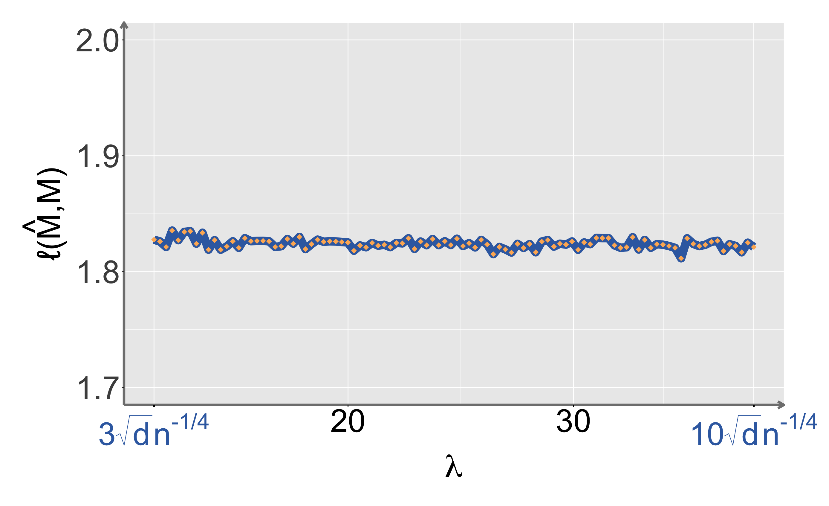
    Experiment 1: n=300n=300, d=250d=250, r=2r=2 (Regime 1). λ\lambda is varying from 3dn−1/43\sqrt{d}n^{-1/4} to 10dn−1/410\sqrt{d}n^{-1/4}.

  • •

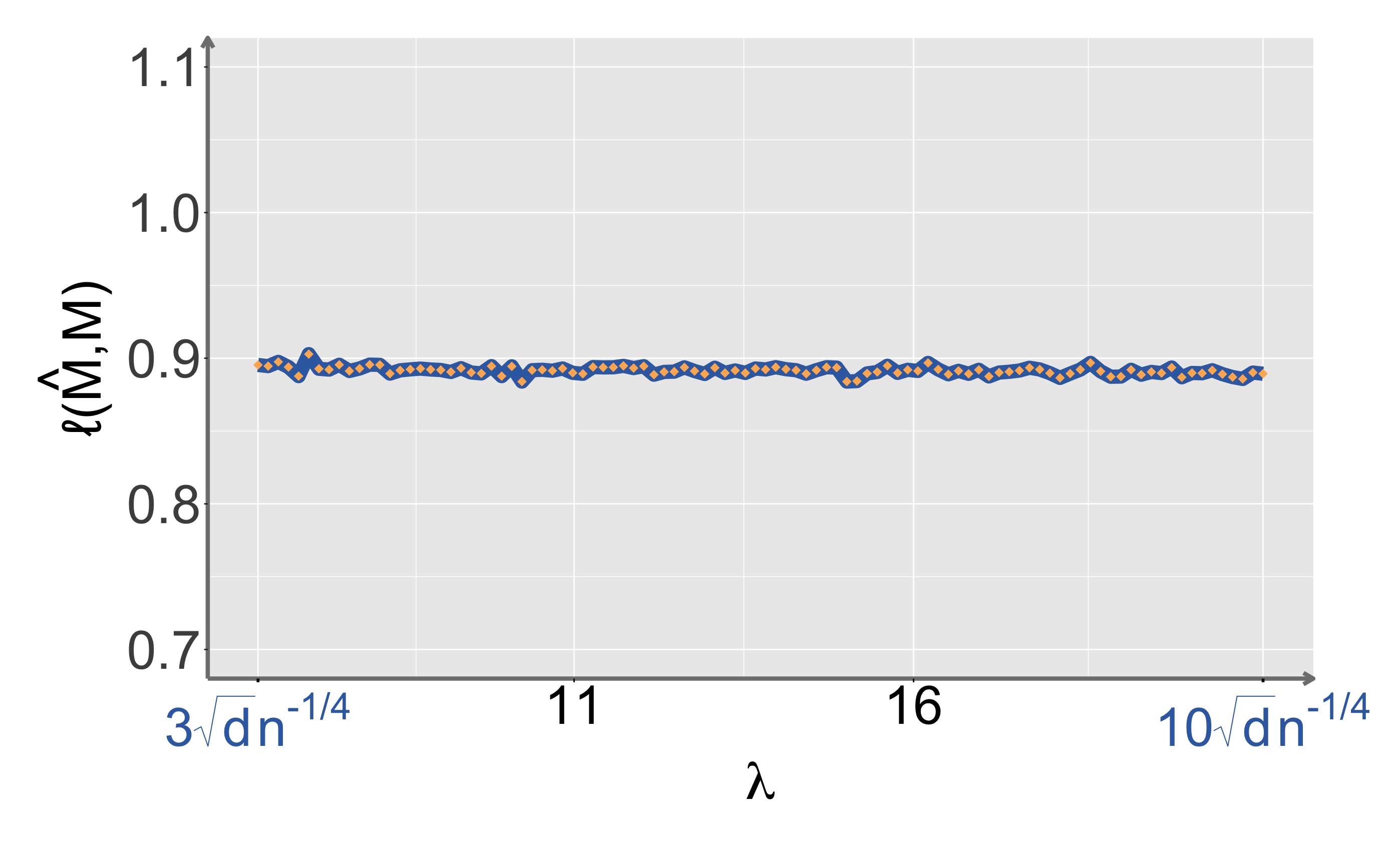
    Experiment 2: n=500n=500, d=100d=100, r=2r=2 (Regime 2). λ\lambda is varying from 3dn−1/43\sqrt{d}n^{-1/4} to 10dn−1/410\sqrt{d}n^{-1/4}.

  • •

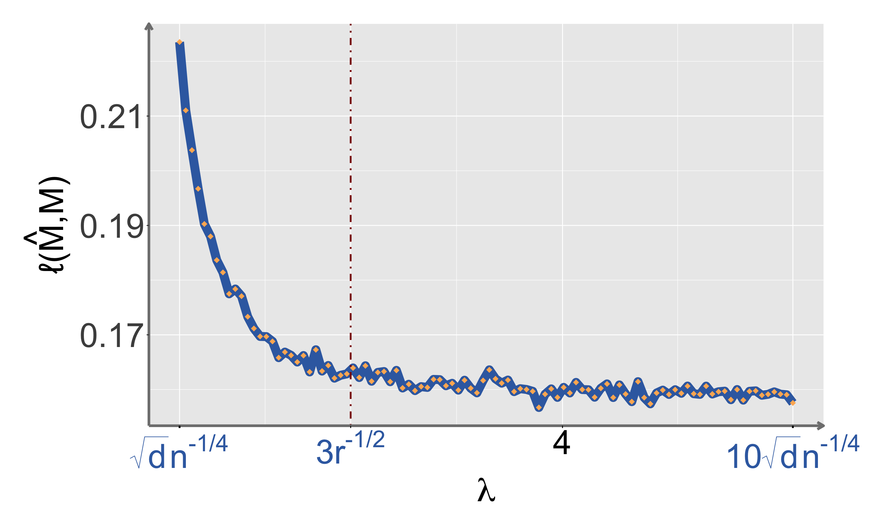
    Experiment 3: n=3000n=3000, d=20d=20, r=2r=2 (Regime 3). λ\lambda is varying from 3dn−1/43\sqrt{d}n^{-1/4} to 10dn−1/410\sqrt{d}n^{-1/4}.

  • •

    Experiment 4: d∈{100,200}d\in\{100,200\}, r=2r=2. nn is varying from 100100 to 10001000 with λ=3dn−1/4\lambda=3\sqrt{d}n^{-1/4}.

  • •

    Experiment 5: n∈{100,200}n\in\{100,200\}, r=2r=2. dd is varying from 100100 to 500500 with λ=3dn−1/4\lambda=3\sqrt{d}n^{-1/4}.

  • •

    Experiment 6: n=10000n=10000, d=10d=10, λ∈{dn−1/4,5}\lambda\in\{\sqrt{d}n^{-1/4},5\} (Regime 3). rr is varying from 22 to 1010.

In Experiment 1 & 2 (Regime 1 & 2), the error stays almost constant as λ\lambda increases. Both cases fall into the strong signal phase and an optimal rate of O⁡((d​r/n)1/2)O((dr/n)^{1/2}) can be attained, suggested by Theorem 3. While in Experiment 3 (Regime 3) with the same range of λ\lambda, the phase transition effect is clearly demonstrated in the bottom panel of Figure 2: when λ\lambda varies from C1d1/2n−1/4C_{1}d^{1/2}n^{-1/4} to C2r−1/2C_{2}r^{-1/2}, the optimal rate O⁡(λ−1​(d/n)1/2)O(\lambda^{-1}(d/n)^{1/2}) is linear in λ−1\lambda^{-1}; when λ≥C2r−1/2\lambda\geq C_{2}r^{-1/2}, the optimal rate O⁡((d​r/n)1/2)O((dr/n)^{1/2}) is again independent of λ\lambda.
In Experiment 4 & 5, we screen the effect of varying nn and dd, respectively in Figure 3. As expected, the error becomes smaller as nn grows (or dd decreases). The linearity between the error rate and n−1/2n^{-1/2} (or d1/2d^{1/2}) can be verified in the right panels, which is in accordance with Theorem 3.
In Experiment 6, we let rr vary with other parameters fixed and focus on Regime 3, which is the most interesting case due to the phase transition effect in terms of rank rr. As shown in Figure 5, the error rate O⁡(λ−1​(d/n)1/2)O(\lambda^{-1}(d/n)^{1/2}) is constant in rr with λ∈(C1d1/2n−1/4,C2r−1/2)\lambda\in(C_{1}d^{1/2}n^{-1/4},C_{2}r^{-1/2}) and when λ≥C2r−1/2\lambda\geq C_{2}r^{-1/2}, the error rate increases with rr.

Refer to caption
Refer to caption
Refer to caption
Figure 2: Experiments with λ\lambda varying. Top-left panel: Regime 1; Top-right panel: Regime 2; Bottom panel: Regime 3.
Refer to caption
Refer to caption
Figure 3: Experiments with nn varying. Left panel: ℓ⁡(^​𝐌,𝐌)\ell(\widehat{}\mathbf{M},\mathbf{M}) against nn; Right panel: ℓ⁡(^​𝐌,𝐌)\ell(\widehat{}\mathbf{M},\mathbf{M}) against n−1/2n^{-1/2}.
Refer to caption
Refer to caption
Figure 4: Experiments with dd varying. Left panel: ℓ⁡(^​𝐌,𝐌)\ell(\widehat{}\mathbf{M},\mathbf{M}) against dd; Right panel: ℓ⁡(^​𝐌,𝐌)\ell(\widehat{}\mathbf{M},\mathbf{M}) against d1/2d^{1/2}.
Refer to caption
Figure 5: Experiments with rr varying. Blue curve λ=d1/2n−1/4\lambda=d^{1/2}n^{-1/4} corresponds to the case where error rate is of order λ−1​(d/n)1/2\lambda^{-1}(d/n)^{1/2}; Red curve λ=5(≥maxrr−1/2)\lambda=5(\geq\max_{r}r^{-1/2}) corresponds to case where the error rate is of order (d​r/n)1/2(dr/n)^{1/2}.

6 Real data experiment

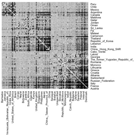
We present an application of our algorithm on a real-world dataset, which is a collection of multiple layers of worldwide food trading networks (De Domenico et al. 2015), recording the trade flows of 30 food products between 99 countries. We pre-process the data the same as in Jing et al. 2021 and end up with a 3-rd order binary tensor 𝓧{\bm{\mathcal{X}}} of dimension 99×99×3099\times 99\times 30. Each layer of this tensor [𝓧]⋅⋅i=𝐗i[{\bm{\mathcal{X}}}]_{\cdot\cdot i}=\mathbf{X}_{i} represents the adjacency matrix of one specific type of food product ii, and nodes are different countries/regions which are common across all layers. As shown in Jing et al. 2021, the layers could be clustered into two groups, one of which mainly consists of raw or unprocessed food and another is made of processed food. We adopt this clustering result as ground truth and assume all layers are generated independently according to two expected adjacency matrices 𝐌1,𝐌2∈ℝ99×99\mathbf{M}_{1},\mathbf{M}_{2}\in\mathbb{R}^{99\times 99}. Note that though throughout the paper the noise matrix 𝐙i\mathbf{Z}_{i} is assumed to be Gaussian , we believe the spectral aggregation can be applied to more general setting (for instance, observations with sub-gaussian noise). Our goal is to recover 𝐌1\mathbf{M}_{1} and 𝐌2\mathbf{M}_{2}. To make it adapted to our framework (as mentioned in Section 1), we first construct centered observations ~​𝐗i=𝐗i−¯​𝐗\widetilde{}\mathbf{X}_{i}=\mathbf{X}_{i}-\bar{}\mathbf{X}, where ¯​𝐗=n−1​∑i=1n𝐗i\bar{}\mathbf{X}=n^{-1}\sum_{i=1}^{n}\mathbf{X}_{i} is the sample average of adjacency matrices over all layers. Here, ¯​𝐗\bar{}\mathbf{X} serves as an estimate of (𝐌1+𝐌2)/2(\mathbf{M}_{1}+\mathbf{M}_{2})/2. Then we apply the spectral aggregation algorithm with rank r=10r=10 to {~​𝐗i}i=1n\{\widetilde{}\mathbf{X}_{i}\}_{i=1}^{n} to get 𝐌^\widehat{\mathbf{M}}. It turns out that the final result is not sensitive to choice of rank rr. Finally we can construct ^​𝐌1=¯​𝐗+𝐌^\widehat{}\mathbf{M}_{1}=\bar{}\mathbf{X}+\widehat{\mathbf{M}} and ^​𝐌2=¯​𝐗−𝐌^\widehat{}\mathbf{M}_{2}=\bar{}\mathbf{X}-\widehat{\mathbf{M}}. To appropriately visualize our result, we rearrange the order of columns and rows of ^​𝐌1\widehat{}\mathbf{M}_{1} and ^​𝐌2\widehat{}\mathbf{M}_{2} in the same way as in Jing et al. 2021, which is based on the community labels estimated by tensor method therein, in order to have a glance of community structures. In Figure 6, the mean matrix in the left panel demonstrates a strong trend of global trading, while the other one shows the dominance of regional trading. These findings coincides with results in Jing et al. 2021, whereas we are estimating the difference of two center matrices instead of clustering all observations. Note that the results in Jing et al. 2021 require layer clustering before producing ^​𝐌1,^​𝐌2\widehat{}\mathbf{M}_{1},\widehat{}\mathbf{M}_{2} but our method does not.

Refer to caption
Refer to caption
Figure 6: Heatmaps for ^​𝐌1\widehat{}\mathbf{M}_{1} and ^​𝐌2\widehat{}\mathbf{M}_{2}.

7 Discussion

Our main focus in this paper is on the optimal estimation and computational limits for the two-component low-rank Gaussian mixtures. It is of great interest to investigate the minimax optimal estimation when the number of components is greater than two. Unfortunately, our spectral aggregation method is inapplicable and we cannot immediately see an easy generalization of the maximum likelihood estimator to the multi-component case. There are several possibilities. For instance, unlike the two-component case, it might be necessary to, at least partially, recover the latent labels before estimating the underlying low-rank components. Indeed, the linear regression low-rank mixture model (Chen et al. 2021) was treated by this way. However, it is well recognized that consistent clustering often requires a much stronger condition on the signal strength. See, for instance, Löffler et al. 2019; Wu and Zhou 2019 and references therein. For the two-component symmetric case as in model (1), consistent clustering requires a signal strength at least88 8 To see this, one can simply assume the singular vectors 𝐔\mathbf{U} and 𝐕\mathbf{V} are available before hand. in the order of Ω⁡(1)\Omega(1) when rr is a constant, which can be much more stringent than the condition required by the spectral aggregation method in Regime 3. It therefore indicates another possibility: there might exist some method that can reliably estimate the multiple low-rank components without the prerequisite of meaningful clustering. We leave this for future works.

References

  • (1) https://www.ncbi.nlm.nih.gov/sites/GDSbrowser?acc=GDS1083.
  • Abramowitz and Stegun (1948) Milton Abramowitz and Irene A Stegun. Handbook of mathematical functions with formulas, graphs, and mathematical tables, volume 55. US Government printing office, 1948.
  • Adamczak (2008) Radoslaw Adamczak. A tail inequality for suprema of unbounded empirical processes with applications to markov chains. Electronic Journal of Probability, 13:1000–1034, 2008.
  • Bakshi et al. (2020) Ainesh Bakshi, Ilias Diakonikolas, He Jia, Daniel M Kane, Pravesh K Kothari, and Santosh S Vempala. Robustly learning mixtures of kk arbitrary gaussians. arXiv preprint arXiv:2012.02119, 2020.
  • Balakrishnan et al. (2017) Sivaraman Balakrishnan, Martin J Wainwright, and Bin Yu. Statistical guarantees for the em algorithm: From population to sample-based analysis. The Annals of Statistics, 45(1):77–120, 2017.
  • Barak and Moitra (2016) Boaz Barak and Ankur Moitra. Noisy tensor completion via the sum-of-squares hierarchy. In Conference on Learning Theory, pages 417–445. PMLR, 2016.
  • Belkin and Sinha (2010) Mikhail Belkin and Kaushik Sinha. Toward learning gaussian mixtures with arbitrary separation. In COLT, pages 407–419, 2010.
  • Cai and Zhang (2018) T Tony Cai and Anru Zhang. Rate-optimal perturbation bounds for singular subspaces with applications to high-dimensional statistics. The Annals of Statistics, 46(1):60–89, 2018.
  • Cai et al. (2013) T Tony Cai, Zongming Ma, and Yihong Wu. Sparse pca: Optimal rates and adaptive estimation. The Annals of Statistics, 41(6):3074–3110, 2013.
  • Cai et al. (2019) T Tony Cai, Jing Ma, and Linjun Zhang. Chime: Clustering of high-dimensional gaussian mixtures with em algorithm and its optimality. The Annals of Statistics, 47(3):1234–1267, 2019.
  • Chen (1995) Jiahua Chen. Optimal rate of convergence for finite mixture models. The Annals of Statistics, pages 221–233, 1995.
  • Chen et al. (2021) Yanxi Chen, Cong Ma, H Vincent Poor, and Yuxin Chena. Learning mixtures of low-rank models. IEEE Transactions on Information Theory, 2021.
  • Cheng et al. (2021) Chen Cheng, Yuting Wei, and Yuxin Chen. Tackling small eigen-gaps: Fine-grained eigenvector estimation and inference under heteroscedastic noise. IEEE Transactions on Information Theory, 67(11):7380–7419, 2021.
  • Davies et al. (2021) Sami Davies, Arya Mazumdar, Soumyabrata Pal, and Cyrus Rashtchian. Lower bounds on the total variation distance between mixtures of two gaussians. arXiv preprint arXiv:2109.01064, 2021.
  • Davis et al. (2021) Damek Davis, Mateo Diaz, and Kaizheng Wang. Clustering a mixture of gaussians with unknown covariance. arXiv preprint arXiv:2110.01602, 2021.
  • De Domenico et al. (2015) Manlio De Domenico, Vincenzo Nicosia, Alexandre Arenas, and Vito Latora. Structural reducibility of multilayer networks. Nature communications, 6(1):1–9, 2015.
  • Do (2003) Minh N Do. Fast approximation of kullback-leibler distance for dependence trees and hidden markov models. IEEE signal processing letters, 10(4):115–118, 2003.
  • Doss et al. (2020) Natalie Doss, Yihong Wu, Pengkun Yang, and Harrison H Zhou. Optimal estimation of high-dimensional location gaussian mixtures. arXiv preprint arXiv:2002.05818, 2020.
  • Gao et al. (2021) Xu Gao, Weining Shen, Liwen Zhang, Jianhua Hu, Norbert J Fortin, Ron D Frostig, and Hernando Ombao. Regularized matrix data clustering and its application to image analysis. Biometrics, 77(3):890–902, 2021.
  • Gavish and Donoho (2014) Matan Gavish and David L Donoho. The optimal hard threshold for singular values is 4/34/\sqrt{3}. IEEE Transactions on Information Theory, 60(8):5040–5053, 2014.
  • Ge et al. (2015) Rong Ge, Qingqing Huang, and Sham M Kakade. Learning mixtures of gaussians in high dimensions. In Proceedings of the forty-seventh annual ACM symposium on Theory of computing, pages 761–770, 2015.
  • Genovese and Wasserman (2000) Christopher R Genovese and Larry Wasserman. Rates of convergence for the gaussian mixture sieve. The Annals of Statistics, 28(4):1105–1127, 2000.
  • Ghosal and Van Der Vaart (2001) Subhashis Ghosal and Aad W Van Der Vaart. Entropies and rates of convergence for maximum likelihood and bayes estimation for mixtures of normal densities. Annals of Statistics, pages 1233–1263, 2001.
  • Golub and van Loan (2013) Gene H. Golub and Charles F. van Loan. Matrix Computations. JHU Press, fourth edition, 2013. ISBN 1421407949 9781421407944. URL http://www.cs.cornell.edu/cv/GVL4/golubandvanloan.htm.
  • Gupta and Nagar (2018) Arjun K Gupta and Daya K Nagar. Matrix variate distributions, volume 104. CRC Press, 2018.
  • Ho and Nguyen (2016a) Nhat Ho and XuanLong Nguyen. Convergence rates of parameter estimation for some weakly identifiable finite mixtures. The Annals of Statistics, 44(6):2726–2755, 2016a.
  • Ho and Nguyen (2016b) Nhat Ho and XuanLong Nguyen. On strong identifiability and convergence rates of parameter estimation in finite mixtures. Electronic Journal of Statistics, 10(1):271–307, 2016b.
  • Hopkins (2018) Samuel Hopkins. Statistical inference and the sum of squares method. PhD thesis, Cornell University, 2018.
  • Hu et al. (2020) Wei Hu, Weining Shen, Hua Zhou, and Dehan Kong. Matrix linear discriminant analysis. Technometrics, 62(2):196–205, 2020.
  • Jing et al. (2021) Bing-Yi Jing, Ting Li, Zhongyuan Lyu, and Dong Xia. Community detection on mixture multilayer networks via regularized tensor decomposition. The Annals of Statistics, 49(6):3181–3205, 2021.
  • Koltchinskii and Lounici (2017) Vladimir Koltchinskii and Karim Lounici. Concentration inequalities and moment bounds for sample covariance operators. Bernoulli, 23(1):110–133, 2017.
  • Koltchinskii and Xia (2015) Vladimir Koltchinskii and Dong Xia. Optimal estimation of low rank density matrices. J. Mach. Learn. Res., 16(53):1757–1792, 2015.
  • Koltchinskii and Xia (2016) Vladimir Koltchinskii and Dong Xia. Perturbation of linear forms of singular vectors under gaussian noise. In High Dimensional Probability VII, pages 397–423. Springer, 2016.
  • Koltchinskii et al. (2011) Vladimir Koltchinskii, Karim Lounici, and Alexandre B Tsybakov. Nuclear-norm penalization and optimal rates for noisy low-rank matrix completion. The Annals of Statistics, 39(5):2302–2329, 2011.
  • Kunisky et al. (2019) Dmitriy Kunisky, Alexander S Wein, and Afonso S Bandeira. Notes on computational hardness of hypothesis testing: Predictions using the low-degree likelihood ratio. arXiv preprint arXiv:1907.11636, 2019.
  • Laurent and Massart (2000) Beatrice Laurent and Pascal Massart. Adaptive estimation of a quadratic functional by model selection. Annals of Statistics, pages 1302–1338, 2000.
  • Le et al. (2018) Can M Le, Keith Levin, and Elizaveta Levina. Estimating a network from multiple noisy realizations. Electronic Journal of Statistics, 12(2):4697–4740, 2018.
  • Ledoux and Talagrand (1991) Michel Ledoux and Michel Talagrand. Probability in Banach Spaces: isoperimetry and processes, volume 23. Springer Science & Business Media, 1991.
  • Leroux (1992) Brian G Leroux. Consistent estimation of a mixing distribution. The Annals of Statistics, pages 1350–1360, 1992.
  • Löffler et al. (2019) Matthias Löffler, Anderson Y Zhang, and Harrison H Zhou. Optimality of spectral clustering in the gaussian mixture model. arXiv preprint arXiv:1911.00538, 2019.
  • Löffler et al. (2020) Matthias Löffler, Alexander S Wein, and Afonso S Bandeira. Computationally efficient sparse clustering. arXiv preprint arXiv:2005.10817, 2020.
  • Lyu et al. (2021) Zhongyuan Lyu, Dong Xia, and Yuan Zhang. Latent space model for higher-order networks and generalized tensor decomposition. arXiv preprint arXiv:2106.16042, 2021.
  • Ma and Wu (2015) Zongming Ma and Yihong Wu. Volume ratio, sparsity, and minimaxity under unitarily invariant norms. IEEE Transactions on Information Theory, 61(12):6939–6956, 2015.
  • Mai et al. (2021) Qing Mai, Xin Zhang, Yuqing Pan, and Kai Deng. A doubly enhanced em algorithm for model-based tensor clustering. Journal of the American Statistical Association, pages 1–15, 2021.
  • Maugis and Michel (2011) Cathy Maugis and Bertrand Michel. A non asymptotic penalized criterion for gaussian mixture model selection. ESAIM: Probability and Statistics, 15:41–68, 2011.
  • Moitra and Valiant (2010) Ankur Moitra and Gregory Valiant. Settling the polynomial learnability of mixtures of gaussians. In 2010 IEEE 51st Annual Symposium on Foundations of Computer Science, pages 93–102. IEEE, 2010.
  • Montanari and Richard (2014) Andrea Montanari and Emile Richard. A statistical model for tensor pca. arXiv preprint arXiv:1411.1076, 2014.
  • Paul and Chen (2020) Subhadeep Paul and Yuguo Chen. Spectral and matrix factorization methods for consistent community detection in multi-layer networks. The Annals of Statistics, 48(1):230–250, 2020.
  • Pearson (1894) Karl Pearson. Contributions to the mathematical theory of evolution. Philosophical Transactions of the Royal Society of London. A, 185:71–110, 1894.
  • Sanjeev and Kannan (2001) Arora Sanjeev and Ravi Kannan. Learning mixtures of arbitrary gaussians. In Proceedings of the thirty-third annual ACM symposium on Theory of computing, pages 247–257, 2001.
  • Sun and Li (2019) Will Wei Sun and Lexin Li. Dynamic tensor clustering. Journal of the American Statistical Association, 114(528):1894–1907, 2019.
  • Tosh and Dasgupta (2017) Christopher Tosh and Sanjoy Dasgupta. Maximum likelihood estimation for mixtures of spherical gaussians is np-hard. J. Mach. Learn. Res., 18:175–1, 2017.
  • Van de Geer (1993) Sara Van de Geer. Hellinger-consistency of certain nonparametric maximum likelihood estimators. The Annals of Statistics, pages 14–44, 1993.
  • Van de Geer (2000) Sara Van de Geer. Empirical Processes in M-estimation, volume 6. Cambridge university press, 2000.
  • Van Der Vaart et al. (1996) Aad W Van Der Vaart, Adrianus Willem van der Vaart, Aad van der Vaart, and Jon Wellner. Weak convergence and empirical processes: with applications to statistics. Springer Science & Business Media, 1996.
  • Vershynin (2010) Roman Vershynin. Introduction to the non-asymptotic analysis of random matrices. arXiv preprint arXiv:1011.3027, 2010.
  • Wainwright (2019) Martin J Wainwright. High-dimensional statistics: A non-asymptotic viewpoint, volume 48. Cambridge University Press, 2019.
  • Wang et al. (2019) Lu Wang, Zhengwu Zhang, and David Dunson. Common and individual structure of brain networks. The Annals of Applied Statistics, 13(1):85–112, 2019.
  • Wang et al. (2017) Xiao Wang, Hongtu Zhu, and Alzheimer’s Disease Neuroimaging Initiative. Generalized scalar-on-image regression models via total variation. Journal of the American Statistical Association, 112(519):1156–1168, 2017.
  • Wu and Yang (2020) Yihong Wu and Pengkun Yang. Optimal estimation of gaussian mixtures via denoised method of moments. The Annals of Statistics, 48(4):1981–2007, 2020.
  • Wu and Zhou (2019) Yihong Wu and Harrison H Zhou. Randomly initialized em algorithm for two-component gaussian mixture achieves near optimality in O⁡(n){O}(\sqrt{n}) iterations. arXiv preprint arXiv:1908.10935, 2019.
  • Xia (2021) Dong Xia. Normal approximation and confidence region of singular subspaces. Electronic Journal of Statistics, 15(2):3798–3851, 2021.
  • Xia and Zhou (2019) Dong Xia and Fan Zhou. The sup-norm perturbation of hosvd and low rank tensor denoising. The Journal of Machine Learning Research, 20(1):2206–2247, 2019.
  • Xia et al. (2021) Dong Xia, Ming Yuan, and Cun-Hui Zhang. Statistically optimal and computationally efficient low rank tensor completion from noisy entries. The Annals of Statistics, 49(1):76–99, 2021.
  • Xu et al. (2016) Ji Xu, Daniel Hsu, and Arian Maleki. Global analysis of expectation maximization for mixtures of two gaussians. arXiv preprint arXiv:1608.07630, 2016.
  • Zadik et al. (2021) Ilias Zadik, Min Jae Song, Alexander S Wein, and Joan Bruna. Lattice-based methods surpass sum-of-squares in clustering. arXiv preprint arXiv:2112.03898, 2021.
  • Zhang and Xia (2018) Anru Zhang and Dong Xia. Tensor svd: Statistical and computational limits. IEEE Transactions on Information Theory, 64(11):7311–7338, 2018.

Appendix A Proofs for main results

A.1 Proof of Theorem 1

For technical reasons discussed in Section 2, we split our proof into two cases, corresponding to the first and second statement in Theorem 1.

Case 1: d​r​log⁡(n​d)<ndr\log(nd)<n

In this regime, the standard tool to establish the convergence rate of MLE is applicable. To this end, we need to introduce the following notations. Define

𝒫¯d1,d2​(r,λ):={p𝐌+p𝐌′2:𝐌′∈ℳd1,d2​(r,λ)},𝒫¯d1,d21/2​(r,λ):={p12:p∈𝒫¯d1,d2​(r,λ)}\bar{\mathcal{P}}_{d_{1},d_{2}}(r,\lambda):=\left\{\frac{p_{\mathbf{M}}+p_{\mathbf{M}^{\prime}}}{2}:\mathbf{M}^{\prime}\in\mathcal{M}_{d_{1},d_{2}}(r,\lambda)\right\},\quad\bar{\mathcal{P}}^{1/2}_{d_{1},d_{2}}(r,\lambda):=\left\{p^{\frac{1}{2}}:p\in\bar{\mathcal{P}}_{d_{1},d_{2}}(r,\lambda)\right\}

and for any small δ>0\delta>0, define a Hellinger ball centered at p𝐌p_{\mathbf{M}} with radius δ\delta by

𝒫¯d1,d21/2​(r,λ,δ):={p¯12∈𝒫¯d1/2​(λ):dH​(p¯,p𝐌)≤δ}\bar{\mathcal{P}}^{1/2}_{d_{1},d_{2}}(r,\lambda,\delta):=\left\{\bar{p}^{\frac{1}{2}}\in\bar{\mathcal{P}}^{1/2}_{d}(\lambda):d_{\textsf{H}}\left(\bar{p},p_{\mathbf{M}}\right)\leq\delta\right\}

We refer to HB​(ϵ,𝒫¯d1,d21/2​(r,λ,δ),L2​(μ))H_{B}(\epsilon,\bar{\mathcal{P}}^{1/2}_{d_{1},d_{2}}(r,\lambda,\delta),L_{2}(\mu)) as the ϵ\epsilon-bracketing entropy of 𝒫¯d1,d21/2​(r,λ,δ)\bar{\mathcal{P}}^{1/2}_{d_{1},d_{2}}(r,\lambda,\delta) under L2​(μ)L_{2}(\mu) metric with Lebesgue measure μ\mu and view 𝒥B​(δ,𝒫¯d1,d21/2​(r,λ,δ),L2​(μ))\mathcal{J}_{B}(\delta,\bar{\mathcal{P}}^{1/2}_{d_{1},d_{2}}(r,\lambda,\delta),L_{2}(\mu)) as the entropy integral of 𝒫¯d1,d21/2​(r,λ,δ)\bar{\mathcal{P}}^{1/2}_{d_{1},d_{2}}(r,\lambda,\delta), which is defined as

𝒥B​(δ,𝒫¯d1,d21/2​(r,λ,δ),L2​(μ)):=∫δ2/213δHB1/2​(ϵ,𝒫¯d1,d21/2​(r,λ,δ),L2​(μ))​𝑑ϵ∨δ\mathcal{J}_{B}(\delta,\bar{\mathcal{P}}^{1/2}_{d_{1},d_{2}}(r,\lambda,\delta),L_{2}(\mu)):=\int_{\delta^{2}/2^{13}}^{\delta}H_{B}^{1/2}(\epsilon,\bar{\mathcal{P}}^{1/2}_{d_{1},d_{2}}(r,\lambda,\delta),L_{2}(\mu))d\epsilon\vee\delta

Now we state Theorem 7.4 in Van de Geer 2000 (adapted to our notation), which establishes the rate of convergence of MLE.

Lemma 3 (Van de Geer 2000).

Take Ψ⁡(δ)≥𝒥B​(δ,𝒫¯d1,d21/2​(r,λ,δ),L2​(μ))\Psi(\delta)\geq\mathcal{J}_{B}(\delta,\bar{\mathcal{P}}^{1/2}_{d_{1},d_{2}}(r,\lambda,\delta),L_{2}(\mu)) in such a way that Ψ⁡(δ)/δ2\Psi(\delta)/\delta^{2} is a non-increasing function of δ\delta. Then for a universal constant cc, and for

n​δn2≥c​Ψ​(δn)\sqrt{n}\delta_{n}^{2}\geq c\Psi(\delta_{n})

we have for all δ≥δn\delta\geq\delta_{n}

ℙ⁡(dH​(p^​𝐌MLE,p𝐌)>δ)≤c​exp⁡(−n​δ2c2)\mathbb{P}(d_{\textsf{H}}(p_{\widehat{}\mathbf{M}_{\textsf{\tiny MLE}}},p_{\mathbf{M}})>\delta)\leq c\exp\left(-\frac{n\delta^{2}}{c^{2}}\right)

A combination of Lemma 1 and Lemma 3 implies that the convergence rate of ^​𝐌MLE\widehat{}\mathbf{M}_{\textsf{\tiny MLE}} would entail an upper bound on the ϵ\epsilon-bracketing entropy HB​(ϵ,𝒫¯d1,d21/2​(r,λ,δ),L2​(μ))H_{B}(\epsilon,\bar{\mathcal{P}}^{1/2}_{d_{1},d_{2}}(r,\lambda,\delta),L_{2}(\mu)). Notice that for any δ>0\delta>0,

HB​(ϵ,𝒫¯d1,d21/2​(r,λ,δ),L2​(μ))\displaystyle H_{B}(\epsilon,\bar{\mathcal{P}}^{1/2}_{d_{1},d_{2}}(r,\lambda,\delta),L_{2}(\mu)) ≤(a)​HB​(ϵ,𝒫¯d1,d21/2​(r,λ),L2​(μ))​=(b)​HB​(ϵ/2,𝒫¯d1,d2​(r,λ),dH)\displaystyle\overset{(a)}{\leq}H_{B}(\epsilon,\bar{\mathcal{P}}^{1/2}_{d_{1},d_{2}}(r,\lambda),L_{2}(\mu))\overset{(b)}{=}H_{B}({\epsilon}/{\sqrt{2}},\bar{\mathcal{P}}_{d_{1},d_{2}}(r,\lambda),d_{\textsf{H}})
≤(c)​HB​(ϵ,𝒫d1,d2​(r,λ),dH)\displaystyle\overset{(c)}{\leq}H_{B}({\epsilon},{\mathcal{P}}_{d_{1},d_{2}}(r,\lambda),d_{\textsf{H}}) (13)

where (a) is due to 𝒫¯d1,d21/2​(r,λ,δ)⊂𝒫¯d1,d21/2​(r,λ)\bar{\mathcal{P}}^{1/2}_{d_{1},d_{2}}(r,\lambda,\delta)\subset\bar{\mathcal{P}}^{1/2}_{d_{1},d_{2}}(r,\lambda), (b) follows from the definition of Hellinger distance dHd_{\textsf{H}} and (c) is due to the following fact (cf. Lemma 4.2 in Van de Geer 2000, Ho and Nguyen 2016a): for any p¯1=12​(p𝐌1+p𝐌)∈𝒫¯d1,d2​(r,λ),p¯2=12​(p𝐌2+p𝐌)∈𝒫¯d1,d2​(r,λ)\bar{p}_{1}=\frac{1}{2}(p_{\mathbf{M}_{1}}+p_{\mathbf{M}})\in\bar{\mathcal{P}}_{d_{1},d_{2}}(r,\lambda),\bar{p}_{2}=\frac{1}{2}(p_{\mathbf{M}_{2}}+p_{\mathbf{M}})\in\bar{\mathcal{P}}_{d_{1},d_{2}}(r,\lambda)

dH2​(p¯1,p¯2)≤12​dH2​(p𝐌1,p𝐌2)d_{\textsf{H}}^{2}(\bar{p}_{1},\bar{p}_{2})\leq\frac{1}{2}d_{\textsf{H}}^{2}(p_{\mathbf{M}_{1}},p_{\mathbf{M}_{2}})

In view of (A.1), it suffices to bound HB​(ϵ,𝒫d1,d2​(r,λ),dH)H_{B}(\epsilon,\mathcal{P}_{d_{1},d_{2}}(r,\lambda),d_{\textsf{H}}). The following lemma characterize the size of bracketing entropy of 𝒫d1,d2​(r,λ)\mathcal{P}_{d_{1},d_{2}}(r,\lambda).

Lemma 4.

Assume d1≍d2≍dd_{1}\asymp d_{2}\asymp d then we have

HB​(ϵ,𝒫d1,d2​(r,λ),dH)≲d​r​log⁡(dϵ)H_{B}(\epsilon,\mathcal{P}_{d_{1},d_{2}}(r,\lambda),d_{\textsf{H}})\lesssim dr\log\left(\frac{d}{\epsilon}\right)

Using relation (A.1) and Lemma 4 we can arrive at

𝒥B​(δ,𝒫¯d1,d21/2​(r,λ,δ),L2​(μ))≲∫δ2/213δd​r​log⁡(dϵ)​𝑑ϵ∨δ≲δ​d​r​log⁡(dδ)\mathcal{J}_{B}(\delta,\bar{\mathcal{P}}^{1/2}_{d_{1},d_{2}}(r,\lambda,\delta),L_{2}(\mu))\lesssim\int_{\delta^{2}/2^{13}}^{\delta}\sqrt{dr\log\left(\frac{d}{\epsilon}\right)}d\epsilon\vee\delta\lesssim\delta\sqrt{dr\log\left(\frac{d}{\delta}\right)}

Now we can take Ψ⁡(δ)=C​δ​d​r​log⁡(dδ)\Psi(\delta)=C\delta\sqrt{dr\log\left(\frac{d}{\delta}\right)} for some absolute constant C>0C>0 and δ=δn=d​rn​log⁡(n​d)\delta=\delta_{n}=\sqrt{\frac{dr}{n}\log(nd)}, then we have Ψ⁡(δ)/δ2=C​1δ​d​r​log⁡(dδ)\Psi(\delta)/\delta^{2}=C\frac{1}{\delta}\sqrt{dr\log\left(\frac{d}{\delta}\right)} is a non-increasing function of δ\delta and that

n​δn2=d​rn​log⁡(n​d)≥c​d​rn​log⁡(n​d)​log⁡(n​dr​log⁡(n​d))=c​Ψ​(δn)\sqrt{n}\delta_{n}^{2}=\frac{dr}{\sqrt{n}}\log(nd)\geq c\frac{dr}{\sqrt{n}}\sqrt{\log(nd)}\sqrt{\log\left(\frac{\sqrt{nd}}{\sqrt{r\log(nd)}}\right)}=c\Psi(\delta_{n})

By Lemma 3, with probability at least 1−exp⁡(−c​d​log2⁡(n​d))1-\exp(-cd\log^{2}(nd)) we have

dH​(p^​𝐌MLE,p𝐌)≤C​d​r​log⁡(n​d)nd_{\textsf{H}}(p_{\widehat{}\mathbf{M}_{\textsf{\tiny MLE}}},p_{\mathbf{M}})\leq C\sqrt{\frac{dr\log(nd)}{n}}

It suffices to use Lemma 1 to connect the density estimation and parameter estimation. Notice that ‖^​𝐌MLE‖F+‖𝐌‖F≍λ​r\|\widehat{}\mathbf{M}_{\textsf{\tiny MLE}}\|_{\rm F}+\|\mathbf{M}\|_{\rm F}\asymp\lambda\sqrt{r}. By Lemma 1, if λ​r≲1\lambda\sqrt{r}\lesssim 1, with probability at least 1−exp⁡(−c​d​log2⁡(n​d))1-\exp(-cd\log^{2}(nd)):

ℓ⁡(^​𝐌MLE,𝐌)≲(λ​r)−1⋅dH​(p^​𝐌MLE,p𝐌)≤1λ​d​log⁡(n​d)n\ell(\widehat{}\mathbf{M}_{\textsf{\tiny MLE}},\mathbf{M})\lesssim(\lambda\sqrt{r})^{-1}\cdot d_{\textsf{H}}(p_{\widehat{}\mathbf{M}_{\textsf{\tiny MLE}}},p_{\mathbf{M}})\leq\frac{1}{\lambda}\sqrt{\frac{d\log(nd)}{n}}

If λ​r≳1\lambda\sqrt{r}\gtrsim 1, note that in this case (d​r<n​log⁡(n​d)dr<n\log(nd)), we have with probability at least 1−exp⁡(−c​d​log2⁡(n​d))1-\exp(-cd\log^{2}(nd)):

min⁡{1,ℓ⁡(^​𝐌MLE,𝐌)}≲dH​(p^​𝐌MLE,p𝐌)≤d​r​log⁡(n​d)n<1\min\{1,\ell(\widehat{}\mathbf{M}_{\textsf{\tiny MLE}},\mathbf{M})\}\lesssim d_{\textsf{H}}(p_{\widehat{}\mathbf{M}_{\textsf{\tiny MLE}}},p_{\mathbf{M}})\leq\sqrt{\frac{dr\log(nd)}{n}}<1

implying that ℓ⁡(^​𝐌MLE,𝐌)≲d​r​log⁡(n​d)/n\ell(\widehat{}\mathbf{M}_{\textsf{\tiny MLE}},\mathbf{M})\lesssim\sqrt{{dr\log(nd)}/{n}}. Combining two pieces we conclude that with probability at least 1−exp⁡(−c​d​log2⁡(n​d))1-\exp(-cd\log^{2}(nd)):

ℓ⁡(^​𝐌MLE,𝐌)≤C⁡(d​r​log⁡(n​d)n∨1λ​d​log⁡(n​d)n)\ell(\widehat{}\mathbf{M}_{\textsf{\tiny MLE}},\mathbf{M})\leq C\left(\sqrt{\frac{dr\log(nd)}{n}}\vee\frac{1}{\lambda}\sqrt{\frac{d\log(nd)}{n}}\right)

We can further have a bound in expectation:

𝔼​ℓ​(^​𝐌MLE,𝐌)≤C⁡(d​r​log⁡(n​d)n∨1λ​d​log⁡(n​d)n)\mathbb{E}\ell(\widehat{}\mathbf{M}_{\textsf{\tiny MLE}},\mathbf{M})\leq C\left(\sqrt{\frac{dr\log(nd)}{n}}\vee\frac{1}{\lambda}\sqrt{\frac{d\log(nd)}{n}}\right)

provided that λ≤exp⁡(c​d​log2⁡(n​d))\lambda\leq\exp(cd\log^{2}(nd)).

Case 2: d​r​log⁡(n​d)≥ndr\log(nd)\geq n

In this regime, our ultimate goal is to have ‖^​𝐌MLE−𝐌‖F≲d​r​log⁡(n​d)/n\|\widehat{}\mathbf{M}_{\textsf{\tiny MLE}}-\mathbf{M}\|_{\rm F}\lesssim\sqrt{dr\log(nd)/n} with high probability and in expectation and hence we can assume ‖^​𝐌MLE−𝐌‖F≥c0​d​r​log⁡(n​d)/n\|\widehat{}\mathbf{M}_{\textsf{\tiny MLE}}-\mathbf{M}\|_{\rm F}\geq c_{0}\sqrt{dr\log(nd)/n} for some absolute constant c0>0c_{0}>0 (otherwise we have the desired result). Without loss of generality, we assume ‖^​𝐌MLE−𝐌‖F≤‖^​𝐌MLE+𝐌‖F\|\widehat{}\mathbf{M}_{\textsf{\tiny MLE}}-\mathbf{M}\|_{\rm F}\leq\|\widehat{}\mathbf{M}_{\textsf{\tiny MLE}}+\mathbf{M}\|_{\rm F}. Unlike Case 1, we resort to KL divergence instead of Hellinger distance to establish the convergence rate. Let P𝐌P_{\mathbf{M}} denote the distribution of (1) and recall the definition of KL divergence, for any 𝐌,𝐌′∈ℳd1,d2​(r,λ)\mathbf{M},\mathbf{M}^{\prime}\in\mathcal{M}_{d_{1},d_{2}}(r,\lambda) we have

DKL(p𝐌∥p𝐌′)=∫(logp𝐌p𝐌′)dP𝐌\displaystyle D_{\textsf{KL}}\left(p_{\mathbf{M}}\big\|p_{\mathbf{M}^{\prime}}\right)=\int\left(\log\frac{p_{\mathbf{M}}}{p_{\mathbf{M}^{\prime}}}\right)dP_{\mathbf{M}}

Note that for fixed 𝐌\mathbf{M} and 𝐌′\mathbf{M}^{\prime}, we simply have DKL(p𝐌∥p𝐌′)=𝔼log(p𝐌(𝐗)/p𝐌′(𝐗))D_{\textsf{KL}}\left(p_{\mathbf{M}}\big\|p_{\mathbf{M}^{\prime}}\right)=\mathbb{E}\log\left({p_{\mathbf{M}}}(\mathbf{X})/{p_{\mathbf{M}^{\prime}}(\mathbf{X})}\right) for 𝐗∼p𝐌\mathbf{X}\sim p_{\mathbf{M}}. On the other hand, by the definition of the maximum likelihood estimator ^​𝐌MLE\widehat{}\mathbf{M}_{\textsf{\tiny MLE}}, we have

1n​∑i=1nlog⁡p𝐌​(𝐗i)p^​𝐌MLE​(𝐗i)≤0\frac{1}{n}\sum_{i=1}^{n}\log\frac{p_{\mathbf{M}}(\mathbf{X}_{i})}{p_{\widehat{}\mathbf{M}_{\textsf{\tiny MLE}}}(\mathbf{X}_{i})}\leq 0

Therefore, we can have that

DKL(p𝐌∥p^​𝐌MLE)≤−1n∑i=1nlogp𝐌​(𝐗i)p^​𝐌MLE​(𝐗i)+DKL(p𝐌∥p^​𝐌MLE)\displaystyle D_{\textsf{KL}}\left(p_{\mathbf{M}}\big\|p_{\widehat{}\mathbf{M}_{\textsf{\tiny MLE}}}\right)\leq-\frac{1}{n}\sum_{i=1}^{n}\log\frac{p_{\mathbf{M}}(\mathbf{X}_{i})}{p_{\widehat{}\mathbf{M}_{\textsf{\tiny MLE}}}(\mathbf{X}_{i})}+D_{\textsf{KL}}\left(p_{\mathbf{M}}\big\|p_{\widehat{}\mathbf{M}_{\textsf{\tiny MLE}}}\right) (14)

Now we give an upper bound of RHS of (14). To this end, we consider a ball in ℳd1,d2​(r,λ)\mathcal{M}_{d_{1},d_{2}}(r,\lambda) with radius δ\delta, i.e., ℳ⁡(δ):={𝐌′∈ℳd1,d2​(r,λ):‖𝐌′−𝐌‖F≤δ}\mathcal{M}(\delta):=\{\mathbf{M}^{\prime}\in\mathcal{M}_{d_{1},d_{2}}(r,\lambda):\|\mathbf{M}^{\prime}-\mathbf{M}\|_{\rm F}\leq\delta\}. Our aim is to bound the following quantity:

θn(δ):=sup𝐌′∈ℳ⁡(δ)|1n∑i=1nlogp𝐌​(𝐗i)p𝐌′​(𝐗i)−DKL(p𝐌∥p𝐌′)|\theta_{n}(\delta):=\sup_{\mathbf{M}^{\prime}\in\mathcal{M}(\delta)}\left|\frac{1}{n}\sum_{i=1}^{n}\log\frac{p_{\mathbf{M}}(\mathbf{X}_{i})}{p_{\mathbf{M}^{\prime}}(\mathbf{X}_{i})}-D_{\textsf{KL}}\left(p_{\mathbf{M}}\big\|p_{\mathbf{M}^{\prime}}\right)\right|

Observe that

log⁡p𝐌​(𝐗)p𝐌′​(𝐗)\displaystyle\log\frac{p_{\mathbf{M}}(\mathbf{X})}{p_{\mathbf{M}^{\prime}}(\mathbf{X})} =log⁡(e−12​‖𝐗−𝐌‖F2+e−12​‖𝐗+𝐌‖F2e−12​‖𝐗−𝐌′‖F2+e−12​‖𝐗+𝐌′‖F2)=12​‖𝐌′‖F2−12​‖𝐌‖F2+log⁡(e⟨𝐗,𝐌⟩+e−⟨𝐗,𝐌⟩e⟨𝐗,𝐌′⟩+e−⟨𝐗,𝐌′⟩)\displaystyle=\log\left(\frac{e^{-\frac{1}{2}\|\mathbf{X}-\mathbf{M}\|_{\rm F}^{2}}+e^{-\frac{1}{2}\|\mathbf{X}+\mathbf{M}\|_{\rm F}^{2}}}{e^{-\frac{1}{2}\|\mathbf{X}-\mathbf{M}^{\prime}\|_{\rm F}^{2}}+e^{-\frac{1}{2}\|\mathbf{X}+\mathbf{M}^{\prime}\|_{\rm F}^{2}}}\right)=\frac{1}{2}\|\mathbf{M}^{\prime}\|_{\rm F}^{2}-\frac{1}{2}\|\mathbf{M}\|_{\rm F}^{2}+\log\left(\frac{e^{\langle\mathbf{X},\mathbf{M}\rangle}+e^{-\langle\mathbf{X},\mathbf{M}\rangle}}{e^{\langle\mathbf{X},\mathbf{M}^{\prime}\rangle}+e^{-\langle\mathbf{X},\mathbf{M}^{\prime}\rangle}}\right)

By log-sum-exp inequality, we have

|⟨𝐗,𝐌⟩|−|⟨𝐗,𝐌′⟩|−log⁡2≤log⁡(e⟨𝐗,𝐌⟩+e−⟨𝐗,𝐌⟩e⟨𝐗,𝐌′⟩+e−⟨𝐗,𝐌′⟩)≤log⁡2+|⟨𝐗,𝐌⟩|−|⟨𝐗,𝐌′⟩|\displaystyle|\langle\mathbf{X},\mathbf{M}\rangle|-|\langle\mathbf{X},\mathbf{M}^{\prime}\rangle|-\log 2\leq\log\left(\frac{e^{\langle\mathbf{X},\mathbf{M}\rangle}+e^{-\langle\mathbf{X},\mathbf{M}\rangle}}{e^{\langle\mathbf{X},\mathbf{M}^{\prime}\rangle}+e^{-\langle\mathbf{X},\mathbf{M}^{\prime}\rangle}}\right)\leq\log 2+|\langle\mathbf{X},\mathbf{M}\rangle|-|\langle\mathbf{X},\mathbf{M}^{\prime}\rangle|

Hence we have

1n∑i=1nlogp𝐌​(𝐗i)p𝐌′​(𝐗i)−DKL(p𝐌∥p𝐌′)≤2log2+1n∑i=1n[|⟨𝐗i,𝐌⟩|−|⟨𝐗i,𝐌′⟩|]−𝔼[|⟨𝐗,𝐌⟩|−|⟨𝐗,𝐌′⟩|]\displaystyle\frac{1}{n}\sum_{i=1}^{n}\log\frac{p_{\mathbf{M}}(\mathbf{X}_{i})}{p_{\mathbf{M}^{\prime}}(\mathbf{X}_{i})}-D_{\textsf{KL}}\left(p_{\mathbf{M}}\big\|p_{\mathbf{M}^{\prime}}\right)\leq 2\log 2+\frac{1}{n}\sum_{i=1}^{n}\left[|\langle\mathbf{X}_{i},\mathbf{M}\rangle|-|\langle\mathbf{X}_{i},\mathbf{M}^{\prime}\rangle|\right]-\mathbb{E}\left[|\langle\mathbf{X},\mathbf{M}\rangle|-|\langle\mathbf{X},\mathbf{M}^{\prime}\rangle|\right]

which implies θn​(δ)≤2​log⁡2+θ~n​(δ)\theta_{n}(\delta)\leq 2\log 2+\tilde{\theta}_{n}(\delta), where

θ~n​(δ):=sup𝐌′∈ℳ⁡(δ)|1n​∑i=1n[|⟨𝐗i,𝐌⟩|−|⟨𝐗i,𝐌′⟩|]−𝔼⁡[|⟨𝐗,𝐌⟩|−|⟨𝐗,𝐌′⟩|]|\displaystyle\tilde{\theta}_{n}(\delta):=\sup_{\mathbf{M}^{\prime}\in\mathcal{M}(\delta)}\left|\frac{1}{n}\sum_{i=1}^{n}\left[|\langle\mathbf{X}_{i},\mathbf{M}\rangle|-|\langle\mathbf{X}_{i},\mathbf{M}^{\prime}\rangle|\right]-\mathbb{E}\left[|\langle\mathbf{X},\mathbf{M}\rangle|-|\langle\mathbf{X},\mathbf{M}^{\prime}\rangle|\right]\right|

To get a high probability bound for θ~n​(δ)\tilde{\theta}_{n}(\delta), we first upper bound its expectation. By symmetrization (see, e.g., in (Van Der Vaart et al. 1996, Lemma 2.3.1)), we have

𝔼​θ~n​(δ)≤2​𝔼​(sup𝐌′∈ℳ⁡(δ)|1n​∑i=1nεi​[|⟨𝐗i,𝐌⟩|−|⟨𝐗i,𝐌′⟩|]|)\displaystyle\mathbb{E}\tilde{\theta}_{n}(\delta)\leq 2\mathbb{E}\left(\sup_{\mathbf{M}^{\prime}\in\mathcal{M}(\delta)}\left|\frac{1}{n}\sum_{i=1}^{n}\varepsilon_{i}\left[|\langle\mathbf{X}_{i},\mathbf{M}\rangle|-|\langle\mathbf{X}_{i},\mathbf{M}^{\prime}\rangle|\right]\right|\right)

where {εi}i=1n\{\varepsilon_{i}\}_{i=1}^{n} are independent Rademacher random variables, which is independent of {𝐗i}i=1n\{\mathbf{X}_{i}\}_{i=1}^{n}. Denote ϕi​(𝐌′)=|⟨𝐗i,𝐌⟩|−|⟨𝐗i,𝐌′⟩|\phi_{i}(\mathbf{M}^{\prime})=|\langle\mathbf{X}_{i},\mathbf{M}\rangle|-|\langle\mathbf{X}_{i},\mathbf{M}^{\prime}\rangle|, for any 𝐌1,𝐌2∈ℳ⁡(δ)\mathbf{M}_{1},\mathbf{M}_{2}\in\mathcal{M}(\delta) we have

|ϕi​(𝐌1)−ϕi​(𝐌2)|≤|⟨𝐗i,𝐌1−𝐌2⟩|=|⟨𝐗i,𝐌1−𝐌⟩−⟨𝐗i,𝐌2−𝐌⟩||\phi_{i}(\mathbf{M}_{1})-\phi_{i}(\mathbf{M}_{2})|\leq|\langle\mathbf{X}_{i},\mathbf{M}_{1}-\mathbf{M}_{2}\rangle|=|\langle\mathbf{X}_{i},\mathbf{M}_{1}-\mathbf{M}\rangle-\langle\mathbf{X}_{i},\mathbf{M}_{2}-\mathbf{M}\rangle|

which means ϕi​(𝐌′)\phi_{i}(\mathbf{M}^{\prime}) is 11-Lipschitz in ⟨𝐗i,𝐌′−𝐌⟩\langle\mathbf{X}_{i},\mathbf{M}^{\prime}-\mathbf{M}\rangle. By comparison theorem ((Ledoux and Talagrand 1991, Theorem 4.12)), we deduce that

𝔼⁡(sup𝐌′∈ℳ⁡(δ)|1n​∑i=1nεi​[|⟨𝐗i,𝐌⟩|−|⟨𝐗i,𝐌′⟩|]|)≤𝔼⁡(sup𝐌′∈ℳ⁡(δ)|1n​∑i=1nεi​⟨𝐗i,𝐌′−𝐌⟩|)\displaystyle\mathbb{E}\left(\sup_{\mathbf{M}^{\prime}\in\mathcal{M}(\delta)}\left|\frac{1}{n}\sum_{i=1}^{n}\varepsilon_{i}\left[|\langle\mathbf{X}_{i},\mathbf{M}\rangle|-|\langle\mathbf{X}_{i},\mathbf{M}^{\prime}\rangle|\right]\right|\right)\leq\mathbb{E}\left(\sup_{\mathbf{M}^{\prime}\in\mathcal{M}(\delta)}\left|\frac{1}{n}\sum_{i=1}^{n}\varepsilon_{i}\langle\mathbf{X}_{i},\mathbf{M}^{\prime}-\mathbf{M}\rangle\right|\right)

Hence we proceed as

𝔼​θ~n​(δ)\displaystyle\mathbb{E}\tilde{\theta}_{n}(\delta) ≤2​𝔼​(sup𝐌′∈ℳ⁡(δ)|1n​∑i=1nεi​⟨𝐗i,𝐌′−𝐌⟩|)=2​𝔼​(sup𝐌′∈ℳ⁡(δ)|1n​∑i=1nεi​⟨si​𝐌+𝐙i,𝐌′−𝐌⟩|)\displaystyle\leq 2\mathbb{E}\left(\sup_{\mathbf{M}^{\prime}\in\mathcal{M}(\delta)}\left|\frac{1}{n}\sum_{i=1}^{n}\varepsilon_{i}\langle\mathbf{X}_{i},\mathbf{M}^{\prime}-\mathbf{M}\rangle\right|\right)=2\mathbb{E}\left(\sup_{\mathbf{M}^{\prime}\in\mathcal{M}(\delta)}\left|\frac{1}{n}\sum_{i=1}^{n}\varepsilon_{i}\langle s_{i}\mathbf{M}+\mathbf{Z}_{i},\mathbf{M}^{\prime}-\mathbf{M}\rangle\right|\right)
≤2​𝔼​(sup𝐌′∈ℳ⁡(δ)|⟨1n​∑i=1nεi​𝐌,𝐌′−𝐌⟩|)+2​𝔼​(sup𝐌′∈ℳ⁡(δ)|⟨1n​∑i=1nεi​𝐙i,𝐌′−𝐌⟩|)\displaystyle\leq 2\mathbb{E}\left(\sup_{\mathbf{M}^{\prime}\in\mathcal{M}(\delta)}\left|\left\langle\frac{1}{n}\sum_{i=1}^{n}\varepsilon_{i}\mathbf{M},\mathbf{M}^{\prime}-\mathbf{M}\right\rangle\right|\right)+2\mathbb{E}\left(\sup_{\mathbf{M}^{\prime}\in\mathcal{M}(\delta)}\left|\left\langle\frac{1}{n}\sum_{i=1}^{n}\varepsilon_{i}\mathbf{Z}_{i},\mathbf{M}^{\prime}-\mathbf{M}\right\rangle\right|\right)
≤(a)​2​δ​‖𝐌‖F​𝔼​|1n​∑i=1nεi|+2​2​r​δ​𝔼​‖1n​∑i=1n𝐙i‖\displaystyle\overset{(a)}{\leq}2\delta\|\mathbf{M}\|_{\rm F}\mathbb{E}\left|\frac{1}{n}\sum_{i=1}^{n}\varepsilon_{i}\right|+2\sqrt{2r}\delta\mathbb{E}\left\|\frac{1}{n}\sum_{i=1}^{n}\mathbf{Z}_{i}\right\|
≤(b)​2​δ​λ​rn+2​2​δ​d​rn​≲(c)​δ​d​rn\displaystyle\overset{(b)}{\leq}2\delta\lambda\sqrt{\frac{r}{n}}+2\sqrt{2}\delta\sqrt{\frac{dr}{n}}\overset{(c)}{\lesssim}\delta\sqrt{\frac{dr}{n}}

where in (a) we’ve used ‖𝐌′−𝐌‖∗≤rank​(𝐌′−𝐌)⋅‖𝐌′−𝐌‖F≤2​r​‖𝐌′−𝐌‖F\|\mathbf{M}^{\prime}-\mathbf{M}\|_{*}\leq\text{rank}(\mathbf{M}^{\prime}-\mathbf{M})\cdot\|\mathbf{M}^{\prime}-\mathbf{M}\|_{\rm F}\leq\sqrt{2r}\|\mathbf{M}^{\prime}-\mathbf{M}\|_{\rm F}, in (b) we have a simple bound for 𝔼​|1n​∑i=1nεi|≤1/n\mathbb{E}\left|\frac{1}{n}\sum_{i=1}^{n}\varepsilon_{i}\right|\leq 1/\sqrt{n} by Jensen’s inequality, and (c) is due to the assumption λ≲d\lambda\lesssim\sqrt{d}. Define σ2:=sup𝐌′∈ℳ⁡(δ)∑i=1n𝔼​[|⟨𝐗i,𝐌⟩|−|⟨𝐗i,𝐌′⟩|]2\sigma^{2}:=\sup_{\mathbf{M}^{\prime}\in\mathcal{M}(\delta)}\sum_{i=1}^{n}\mathbb{E}\left[|\langle\mathbf{X}_{i},\mathbf{M}\rangle|-|\langle\mathbf{X}_{i},\mathbf{M}^{\prime}\rangle|\right]^{2}, notice that

[|⟨𝐗i,𝐌⟩|−|⟨𝐗i,𝐌′⟩|]2\displaystyle\left[|\langle\mathbf{X}_{i},\mathbf{M}\rangle|-|\langle\mathbf{X}_{i},\mathbf{M}^{\prime}\rangle|\right]^{2} ≤|⟨𝐗i,𝐌−𝐌′⟩|2=|⟨si​𝐌+𝐙i,𝐌−𝐌′⟩|2\displaystyle\leq|\langle\mathbf{X}_{i},\mathbf{M}-\mathbf{M}^{\prime}\rangle|^{2}=|\langle s_{i}\mathbf{M}+\mathbf{Z}_{i},\mathbf{M}-\mathbf{M}^{\prime}\rangle|^{2}
=⟨𝐌,𝐌−𝐌′⟩2+⟨𝐙i,𝐌−𝐌′⟩2+2​si​⟨𝐌,𝐌−𝐌′⟩​⟨𝐙i,𝐌−𝐌′⟩\displaystyle=\langle\mathbf{M},\mathbf{M}-\mathbf{M}^{\prime}\rangle^{2}+\langle\mathbf{Z}_{i},\mathbf{M}-\mathbf{M}^{\prime}\rangle^{2}+2s_{i}\langle\mathbf{M},\mathbf{M}-\mathbf{M}^{\prime}\rangle\langle\mathbf{Z}_{i},\mathbf{M}-\mathbf{M}^{\prime}\rangle

Observe that ⟨𝐙i,𝐌−𝐌′⟩∼𝒩⁡(0,‖𝐌−𝐌′‖F2)\langle\mathbf{Z}_{i},\mathbf{M}-\mathbf{M}^{\prime}\rangle\sim\mathcal{N}(0,\|\mathbf{M}-\mathbf{M}^{\prime}\|_{\rm F}^{2}), we have σ2≤n​‖𝐌‖F2​δ2+n​δ2≲n​λ2​r​δ2\sigma^{2}\leq n\|\mathbf{M}\|_{\rm F}^{2}\delta^{2}+n\delta^{2}\lesssim n\lambda^{2}r\delta^{2}, the last inequality is due to ‖𝐌‖F≥λ​r≳1\|\mathbf{M}\|_{\rm F}\geq\lambda\sqrt{r}\gtrsim 1 in this regime. Moreover, by Lemma 2.2.2 in Van Der Vaart et al. 1996, we have

‖max⁡sup𝐌′∈ℳ⁡(δ)i⁡|ϕi​(𝐌′)−𝔼​ϕi​(𝐌′)|‖ψ2≲log⁡n​maxi​‖sup𝐌′∈ℳ⁡(δ)|ϕi​(𝐌′)−𝔼​ϕi​(𝐌′)|‖ψ2\displaystyle\left\|\max_{i}\sup_{\mathbf{M}^{\prime}\in\mathcal{M}(\delta)}\left|\phi_{i}(\mathbf{M}^{\prime})-\mathbb{E}\phi_{i}(\mathbf{M}^{\prime})\right|\right\|_{\psi_{2}}\lesssim\sqrt{\log n}\max_{i}\left\|\sup_{\mathbf{M}^{\prime}\in\mathcal{M}(\delta)}\left|\phi_{i}(\mathbf{M}^{\prime})-\mathbb{E}\phi_{i}(\mathbf{M}^{\prime})\right|\right\|_{\psi_{2}}

It suffices to note that for each i∈[n]i\in[n],

sup𝐌′∈ℳ⁡(δ)|ϕi​(𝐌′)−𝔼​ϕi​(𝐌′)|\displaystyle\sup_{\mathbf{M}^{\prime}\in\mathcal{M}(\delta)}\left|\phi_{i}(\mathbf{M}^{\prime})-\mathbb{E}\phi_{i}(\mathbf{M}^{\prime})\right| ≤sup𝐌′∈ℳ⁡(δ)|⟨𝐗i,𝐌′−𝐌⟩|+sup𝐌′∈ℳ⁡(δ)𝔼​|⟨𝐗i,𝐌′−𝐌⟩|\displaystyle\leq\sup_{\mathbf{M}^{\prime}\in\mathcal{M}(\delta)}\left|\langle\mathbf{X}_{i},\mathbf{M}^{\prime}-\mathbf{M}\rangle\right|+\sup_{\mathbf{M}^{\prime}\in\mathcal{M}(\delta)}\mathbb{E}\left|\langle\mathbf{X}_{i},\mathbf{M}^{\prime}-\mathbf{M}\rangle\right|
≤δ​‖𝐌‖F+δ​r​‖𝐙i‖+𝔼⁡(δ​‖𝐌‖F+δ​r​‖𝐙i‖)\displaystyle\leq\delta\|\mathbf{M}\|_{\rm F}+\delta\sqrt{r}\|\mathbf{Z}_{i}\|+\mathbb{E}\left(\delta\|\mathbf{M}\|_{\rm F}+\delta\sqrt{r}\|\mathbf{Z}_{i}\|\right)
≲δ​d​r+δ​r​‖𝐙i‖\displaystyle\lesssim\delta\sqrt{dr}+\delta\sqrt{r}\|\mathbf{Z}_{i}\|

where in the last inequality we’ve used 𝔼​‖𝐙i‖≲d\mathbb{E}\|\mathbf{Z}_{i}\|\lesssim\sqrt{d} and λ≲d\lambda\lesssim\sqrt{d}. By random matrix theory, we know 𝔼​‖𝐙i‖≍d\mathbb{E}\|\mathbf{Z}_{i}\|\asymp\sqrt{d} and ‖𝐙i‖−𝔼​‖𝐙i‖\|\mathbf{Z}_{i}\|-\mathbb{E}\|\mathbf{Z}_{i}\| is sub-gaussian, then ‖‖𝐙i‖‖ψ2≲d\|\|\mathbf{Z}_{i}\|\|_{\psi_{2}}\lesssim\sqrt{d}. Hence

‖max⁡sup𝐌′∈ℳ⁡(δ)i⁡|ϕi​(𝐌′)−𝔼​ϕi​(𝐌′)|‖ψ2≲δ​d​r​log⁡n+δ​r​log⁡n​maxi​‖‖𝐙i‖‖ψ2≲δ​d​r​log⁡n\displaystyle\left\|\max_{i}\sup_{\mathbf{M}^{\prime}\in\mathcal{M}(\delta)}\left|\phi_{i}(\mathbf{M}^{\prime})-\mathbb{E}\phi_{i}(\mathbf{M}^{\prime})\right|\right\|_{\psi_{2}}\lesssim\delta\sqrt{dr\log n}+\delta\sqrt{r\log n}\max_{i}\left\|\|\mathbf{Z}_{i}\|\right\|_{\psi_{2}}\lesssim\delta\sqrt{dr\log n}

Now we can invoke concentration inequality for suprema of empirical processes of unbounded functions (Adamczak 2008, Theorem 4), we have for any t≥0t\geq 0:

ℙ⁡(θ~n​(δ)≥C​δ​d​r​log⁡nn+δ​d​rn​t)≤exp⁡(−c​t2)\displaystyle\mathbb{P}\left(\tilde{\theta}_{n}(\delta)\geq C\delta\sqrt{\frac{dr\log n}{n}}+\delta\sqrt{\frac{dr}{n}}t\right)\leq\exp\left(-ct^{2}\right) (15)

Note that (15) only holds for any given δ>0\delta>0. Consider any δ∈[d​r/n,2​d​r]\delta\in[\sqrt{dr/n},2\sqrt{dr}], let δj=2j​d​r/n\delta_{j}=2^{j}\sqrt{dr/n} for j=0,1,⋯,k∗+1j=0,1,\cdots,k^{*}+1 with k∗:=⌊log2⁡(2​n)⌋k^{*}:=\lfloor\log_{2}(2\sqrt{n})\rfloor, then δ∈⋃j=1k∗[δj,δj+1]\delta\in\bigcup_{j=1}^{k^{*}}[\delta_{j},\delta_{j+1}]. By construction, for any δ∈[δj,δj+1]\delta\in[\delta_{j},\delta_{j+1}], we have δ≍δj≍δj+1\delta\asymp\delta_{j}\asymp\delta_{j+1}. Hence for fixed jj, (15) holds for any δ∈[δj,δj+1]\delta\in[\delta_{j},\delta_{j+1}] up to change in constants c>0c>0 and C>0C>0. Take a union bound over all j=0,1,⋯,k∗+1j=0,1,\cdots,k^{*}+1, we have (15) holds for any δ∈[d​r/n,2​d​r]\delta\in[\sqrt{dr/n},2\sqrt{dr}] and any t≥log⁡(k∗+2)≳log⁡log⁡nt\geq\log(k^{*}+2)\gtrsim\log\log n. Combined with (14), we conclude that

DKL(p𝐌∥p^​𝐌MLE)\displaystyle D_{\textsf{KL}}\left(p_{\mathbf{M}}\big\|p_{\widehat{}\mathbf{M}_{\textsf{\tiny MLE}}}\right) ≤|1n∑i=1nlogp𝐌​(𝐗i)p^​𝐌MLE​(𝐗i)−DKL(p𝐌∥p^​𝐌MLE)|≤θ~n(∥^𝐌MLE−𝐌∥F)+2log2\displaystyle\leq\left|\frac{1}{n}\sum_{i=1}^{n}\log\frac{p_{\mathbf{M}}(\mathbf{X}_{i})}{p_{\widehat{}\mathbf{M}_{\textsf{\tiny MLE}}}(\mathbf{X}_{i})}-D_{\textsf{KL}}\left(p_{\mathbf{M}}\big\|p_{\widehat{}\mathbf{M}_{\textsf{\tiny MLE}}}\right)\right|\leq\tilde{\theta}_{n}(\|\widehat{}\mathbf{M}_{\textsf{\tiny MLE}}-\mathbf{M}\|_{\rm F})+2\log 2
≤C​‖^​𝐌MLE−𝐌‖F​d​r​log⁡(n​d)n\displaystyle\leq C\|\widehat{}\mathbf{M}_{\textsf{\tiny MLE}}-\mathbf{M}\|_{\rm F}\sqrt{\frac{dr\log(nd)}{n}} (16)

where the last inequality holds with probability at least 1−(n​d)−41-(nd)^{-4}, due to the facts that ‖^​𝐌MLE−𝐌‖F≳d​r​log⁡(n​d)/n≥1\|\widehat{}\mathbf{M}_{\textsf{\tiny MLE}}-\mathbf{M}\|_{\rm F}\gtrsim\sqrt{dr\log(nd)/n}\geq 1. Since ‖^​𝐌MLE−𝐌‖F≳1\|\widehat{}\mathbf{M}_{\textsf{\tiny MLE}}-\mathbf{M}\|_{\rm F}\gtrsim 1 and ‖𝐌‖F≳1\|\mathbf{M}\|_{\rm F}\gtrsim 1 in this regime, it turns out that we can apply Lemma 2 to get a lower bound of DKL(p𝐌∥p^​𝐌MLE)D_{\textsf{KL}}\left(p_{\mathbf{M}}\big\|p_{\widehat{}\mathbf{M}_{\textsf{\tiny MLE}}}\right), hence we have with probability at least 1−(n​d)−41-(nd)^{-4} that

‖^​𝐌MLE−𝐌‖F≤C​d​r​log⁡(n​d)n\displaystyle\|\widehat{}\mathbf{M}_{\textsf{\tiny MLE}}-\mathbf{M}\|_{\rm F}\leq C\sqrt{\frac{dr\log(nd)}{n}}

Finally, we can have a bound in expectation

𝔼​‖^​𝐌MLE−𝐌‖F≤C​d​r​log⁡(n​d)n\displaystyle\mathbb{E}\|\widehat{}\mathbf{M}_{\textsf{\tiny MLE}}-\mathbf{M}\|_{\rm F}\leq C\sqrt{\frac{dr\log(nd)}{n}}

given that λ≲d\lambda\lesssim\sqrt{d}. ∎

A.2 Proof of Theorem 3

In the proof, we consider the conditional model with sample splitting, i.e., 𝐗i(k)​=𝑑​si(k)​𝐌+𝐙i(k)\mathbf{X}_{i}^{(k)}\overset{d}{=}s_{i}^{(k)}\mathbf{M}+\mathbf{Z}_{i}^{(k)} for k=1,2,3,4k=1,2,3,4 and i∈[n0]i\in[n_{0}]. Let 𝐔​𝚺​𝐕⊤\mathbf{U}\mathbf{\Sigma}\mathbf{V}^{\top} denote the thin SVD of the signal matrix 𝐌\mathbf{M} and recall that d1≍d2≍dd_{1}\asymp d_{2}\asymp d.

Step 1:

Denote 𝐗f=[𝐗1(1),⋯,𝐗n0(1)]∈ℝd×n0​d\mathbf{X}_{f}=[\mathbf{X}_{1}^{(1)},\cdots,\mathbf{X}_{n_{0}}^{(1)}]\in\mathbb{R}^{d\times{n_{0}}d}. A key observation is that ^​𝐮1\widehat{}\mathbf{u}_{1} is also the leading eigenvector of 1n0​𝐗f​𝐗f⊤−d​𝐈d\frac{1}{n_{0}}\mathbf{X}_{f}\mathbf{X}_{f}^{\top}-d\mathbf{I}_{d}. Then we have

1n0​𝐗f​𝐗f⊤−d​𝐈d\displaystyle\frac{1}{n_{0}}\mathbf{X}_{f}\mathbf{X}_{f}^{\top}-d\mathbf{I}_{d} =1n0​∑i=1n0𝐗i(1)​𝐗i(1)⊤−d​𝐈d=𝐌𝐌⊤+Δ\displaystyle=\frac{1}{n_{0}}\sum_{i=1}^{n_{0}}\mathbf{X}_{i}^{(1)}\mathbf{X}_{i}^{(1)\top}-d\mathbf{I}_{d}=\mathbf{M}\mathbf{M}^{\top}+\Delta (17)

where

Δ:=𝐌⁡(1n0​∑i=1n0si(1)​𝐙i(1)⊤)+(1n0​∑i=1n0si(1)​𝐙i(1))​𝐌⊤+1n0​∑i=1n0𝐙i(1)​𝐙i(1)⊤−d​𝐈d1\Delta:=\mathbf{M}\left(\frac{1}{n_{0}}\sum_{i=1}^{n_{0}}s_{i}^{(1)}\mathbf{Z}_{i}^{(1)\top}\right)+\left(\frac{1}{n_{0}}\sum_{i=1}^{n_{0}}s_{i}^{(1)}\mathbf{Z}_{i}^{(1)}\right)\mathbf{M}^{\top}+\frac{1}{n_{0}}\sum_{i=1}^{n_{0}}\mathbf{Z}_{i}^{(1)}\mathbf{Z}_{i}^{(1)\top}-d\mathbf{I}_{d_{1}}

Note that ∑i=1n0si(1)​𝐙i(1)\sum_{i=1}^{n_{0}}s_{i}^{(1)}\mathbf{Z}_{i}^{(1)} (∑i=1n0si(1)​𝐙i(1)⊤\sum_{i=1}^{n_{0}}s_{i}^{(1)}\mathbf{Z}_{i}^{(1)\top}) is a d1×d2d_{1}\times d_{2} (d2×d1d_{2}\times d_{1}) matrix of independent centered Gaussian entries with variance n0n_{0}, then by random matrix theory (e.g. Vershynin 2010) with probability at least 1−exp⁡(−c​d)1-\exp(-cd), we have:

‖𝐌⁡(1n0​∑i=1n0si(1)​𝐙i(1)⊤)‖≲λ1​dn,‖(1n0​∑i=1n0si(1)​𝐙i(1))​𝐌⊤‖≲λ1​dn\left\|\mathbf{M}\left(\frac{1}{n_{0}}\sum_{i=1}^{n_{0}}s_{i}^{(1)}\mathbf{Z}_{i}^{(1)\top}\right)\right\|\lesssim\lambda_{1}\sqrt{\frac{d}{n}},\quad\left\|\left(\frac{1}{n_{0}}\sum_{i=1}^{n_{0}}s_{i}^{(1)}\mathbf{Z}_{i}^{(1)}\right)\mathbf{M}^{\top}\right\|\lesssim\lambda_{1}\sqrt{\frac{d}{n}}

Furthermore, since

1n0∑i=1n0𝐙i(1)𝐙i(1)⊤−d𝐈d1=d(1n0​d∑i=1n0∑j=1d[𝐙i(1)]:j[𝐙i(1)]:j⊤−𝐈d1)\displaystyle\frac{1}{n_{0}}\sum_{i=1}^{n_{0}}\mathbf{Z}_{i}^{(1)}\mathbf{Z}_{i}^{(1)\top}-d\mathbf{I}_{d_{1}}=d\left(\frac{1}{n_{0}d}\sum_{i=1}^{n_{0}}\sum_{j=1}^{d}[\mathbf{Z}_{i}^{(1)}]_{:j}[\mathbf{Z}_{i}^{(1)}]^{\top}_{:j}-\mathbf{I}_{d_{1}}\right)

where [𝐙i(1)]:j[\mathbf{Z}_{i}^{(1)}]_{:j} is the jj-th column of 𝐙i(1)\mathbf{Z}_{i}^{(1)}. By concentration of sample covariance operator (e.g. Koltchinskii and Lounici 2017), we have with probability at least 1−exp⁡(−c​d)1-\exp(-cd):

‖d(1n0​d∑i=1n0∑j=1d[𝐙i(1)]:j[𝐙i(1)]:j⊤−𝐈d1)‖≲dn\displaystyle\left\|d\left(\frac{1}{n_{0}d}\sum_{i=1}^{n_{0}}\sum_{j=1}^{d}[\mathbf{Z}_{i}^{(1)}]_{:j}[\mathbf{Z}_{i}^{(1)}]^{\top}_{:j}-\mathbf{I}_{d_{1}}\right)\right\|\lesssim\frac{d}{\sqrt{n}}

By (17) and eigenvalue perturbation theory (e.g. Corollary 8.1.6 in Golub and van Loan 2013), we have99 9 With slight abuse of notation, we use λj​(⋅)\lambda_{j}(\cdot) to denote the jj-th largest eigenvalue of a given matrix, while λj\lambda_{j}’s themselves are singular values of 𝐌\mathbf{M}.

λ12−‖Δ‖≤λ1​(1n0​𝐗f​𝐗f⊤−d​𝐈d1)≤λ12+‖Δ‖\displaystyle\lambda_{1}^{2}-\|\Delta\|\leq\lambda_{1}\left(\frac{1}{n_{0}}\mathbf{X}_{f}\mathbf{X}_{f}^{\top}-d\mathbf{I}_{d_{1}}\right)\leq\lambda_{1}^{2}+\|\Delta\|

Therefore, we obtain

λ12−2​‖Δ‖≤^​𝐮1⊤​𝐌𝐌⊤​^​𝐮1≤λ12+2​‖Δ‖\displaystyle\lambda_{1}^{2}-2\|\Delta\|\leq\widehat{}\mathbf{u}_{1}^{\top}\mathbf{M}\mathbf{M}^{\top}\widehat{}\mathbf{u}_{1}\leq\lambda_{1}^{2}+2\|\Delta\| (18)

Hence with probability at least 1−exp⁡(−c​d)1-\exp(-cd) we have

^​𝐮1⊤​𝐌𝐌⊤​^​𝐮1≥λ12−2​‖Δ‖≥λ12−C⁡(λ1​dn+dn)≳λ12\displaystyle\widehat{}\mathbf{u}_{1}^{\top}\mathbf{M}\mathbf{M}^{\top}\widehat{}\mathbf{u}_{1}\geq\lambda_{1}^{2}-2\|\Delta\|\geq\lambda_{1}^{2}-C\left(\lambda_{1}\sqrt{\frac{d}{n}}+\frac{d}{\sqrt{n}}\right)\gtrsim\lambda_{1}^{2} (19)

where the last inequality holds provided that λ2≥C0​dn\lambda^{2}\geq C_{0}\frac{d}{\sqrt{n}} for some large absolute constant C0>0C_{0}>0.

Step 2:

Observe that ^​𝐯1\widehat{}\mathbf{v}_{1} is the leading eigenvector of 1n0​∑i=1n0𝐗i(2)⊤​^​𝐮1​^​𝐮1⊤​𝐗i(2)−𝐈d2\frac{1}{n_{0}}\sum_{i=1}^{n_{0}}\mathbf{X}_{i}^{(2)\top}\widehat{}\mathbf{u}_{1}\widehat{}\mathbf{u}_{1}^{\top}\mathbf{X}_{i}^{(2)}-\mathbf{I}_{d_{2}} and we have the following decomposition:

1n0​∑i=1n0𝐗i(2)⊤​^​𝐮1​^​𝐮1⊤​𝐗i(2)−𝐈d2=𝐌⊤​^​𝐮1​^​𝐮1⊤​𝐌+Δ′\displaystyle\frac{1}{n_{0}}\sum_{i=1}^{n_{0}}\mathbf{X}_{i}^{(2)\top}\widehat{}\mathbf{u}_{1}\widehat{}\mathbf{u}_{1}^{\top}\mathbf{X}_{i}^{(2)}-\mathbf{I}_{d_{2}}=\mathbf{M}^{\top}\widehat{}\mathbf{u}_{1}\widehat{}\mathbf{u}_{1}^{\top}\mathbf{M}+\Delta^{\prime} (20)

where

Δ′:=(1n0​∑i=1n0si(2)​𝐙i(2)⊤​^​𝐮1)​^​𝐮1⊤​𝐌+𝐌⊤​^​𝐮1​(1n0​∑i=1n0^​𝐮1⊤​si(2)​𝐙i(2))+1n0​∑i=1n0𝐙i(2)⊤​^​𝐮1​^​𝐮1⊤​𝐙i(2)−𝐈d2\Delta^{\prime}:=\left(\frac{1}{n_{0}}\sum_{i=1}^{n_{0}}s_{i}^{(2)}\mathbf{Z}_{i}^{(2)\top}\widehat{}\mathbf{u}_{1}\right)\widehat{}\mathbf{u}_{1}^{\top}\mathbf{M}+\mathbf{M}^{\top}\widehat{}\mathbf{u}_{1}\left(\frac{1}{n_{0}}\sum_{i=1}^{n_{0}}\widehat{}\mathbf{u}_{1}^{\top}s_{i}^{(2)}\mathbf{Z}_{i}^{(2)}\right)+\frac{1}{n_{0}}\sum_{i=1}^{n_{0}}\mathbf{Z}_{i}^{(2)\top}\widehat{}\mathbf{u}_{1}\widehat{}\mathbf{u}_{1}^{\top}\mathbf{Z}_{i}^{(2)}-\mathbf{I}_{d_{2}}

Due to the independence of ^​𝐮1\widehat{}\mathbf{u}_{1} and {𝐙i(2)}i=1n0\{\mathbf{Z}_{i}^{(2)}\}_{i=1}^{n_{0}}, we conclude that 1n0​∑i=1n0si(2)​𝐙i(2)⊤​^​𝐮1∼𝒩⁡(0,1n0​𝐈d2)\frac{1}{n_{0}}\sum_{i=1}^{n_{0}}s_{i}^{(2)}\mathbf{Z}_{i}^{(2)\top}\widehat{}\mathbf{u}_{1}\sim{\cal N}(0,\frac{1}{n_{0}}\mathbf{I}_{d_{2}}), hence with probability at least 1−exp⁡(−c​d)1-\exp(-cd):

‖(1n0​∑i=1n0si(2)​𝐙i(2)⊤​^​𝐮1)​^​𝐮1⊤​𝐌‖≲λ1​dn,‖𝐌⊤​^​𝐮1​(1n0​∑i=1n0^​𝐮1⊤​si(2)​𝐙i(2))‖≲λ1​dn\displaystyle\left\|\left(\frac{1}{n_{0}}\sum_{i=1}^{n_{0}}s_{i}^{(2)}\mathbf{Z}_{i}^{(2)\top}\widehat{}\mathbf{u}_{1}\right)\widehat{}\mathbf{u}_{1}^{\top}\mathbf{M}\right\|\lesssim\lambda_{1}\sqrt{\frac{d}{n}},\quad\left\|\mathbf{M}^{\top}\widehat{}\mathbf{u}_{1}\left(\frac{1}{n_{0}}\sum_{i=1}^{n_{0}}\widehat{}\mathbf{u}_{1}^{\top}s_{i}^{(2)}\mathbf{Z}_{i}^{(2)}\right)\right\|\lesssim\lambda_{1}\sqrt{\frac{d}{n}}

Notice that 1n0​∑i=1n0𝐙i(2)⊤​^​𝐮1​^​𝐮1⊤​𝐙i(2)​=𝑑​1n0​∑i=1n0𝐳i​𝐳i⊤\frac{1}{n_{0}}\sum_{i=1}^{n_{0}}\mathbf{Z}_{i}^{(2)\top}\widehat{}\mathbf{u}_{1}\widehat{}\mathbf{u}_{1}^{\top}\mathbf{Z}_{i}^{(2)}\overset{d}{=}\frac{1}{n_{0}}\sum_{i=1}^{n_{0}}\mathbf{z}_{i}\mathbf{z}_{i}^{\top}, where 𝐳i∼𝒩⁡(0,𝐈d2)\mathbf{z}_{i}\sim{\cal N}(0,\mathbf{I}_{d_{2}}) and 𝐳i\mathbf{z}_{i}’s are independent. Again, by concentration of sample covariance operator, with probability at least 1−exp⁡(−c​d)1-\exp(-cd):

‖1n0​∑i=1n0𝐙i(2)⊤​^​𝐮1​^​𝐮1⊤​𝐙i(2)−𝐈d2‖≲dn∨dn\displaystyle\left\|\frac{1}{n_{0}}\sum_{i=1}^{n_{0}}\mathbf{Z}_{i}^{(2)\top}\widehat{}\mathbf{u}_{1}\widehat{}\mathbf{u}_{1}^{\top}\mathbf{Z}_{i}^{(2)}-\mathbf{I}_{d_{2}}\right\|\lesssim\sqrt{\frac{d}{n}}\vee\frac{d}{n}

Therefore, (20) and eigenvalue perturbation theory imply that

λ1​(𝐌⊤​^​𝐮1​^​𝐮1⊤​𝐌)−‖Δ′‖≤λ1​(1n0​∑i=1n0𝐗i(2)⊤​^​𝐮1​^​𝐮1⊤​𝐗i(2)−𝐈d2)≤λ1​(𝐌⊤​^​𝐮1​^​𝐮1⊤​𝐌)+‖Δ′‖\displaystyle\lambda_{1}\left(\mathbf{M}^{\top}\widehat{}\mathbf{u}_{1}\widehat{}\mathbf{u}_{1}^{\top}\mathbf{M}\right)-\|\Delta^{\prime}\|\leq\lambda_{1}\left(\frac{1}{n_{0}}\sum_{i=1}^{n_{0}}\mathbf{X}_{i}^{(2)\top}\widehat{}\mathbf{u}_{1}\widehat{}\mathbf{u}_{1}^{\top}\mathbf{X}_{i}^{(2)}-\mathbf{I}_{d_{2}}\right)\leq\lambda_{1}\left(\mathbf{M}^{\top}\widehat{}\mathbf{u}_{1}\widehat{}\mathbf{u}_{1}^{\top}\mathbf{M}\right)+\|\Delta^{\prime}\|

Combined with the decomposition (20), we can arrive at

λ12−2​(‖Δ‖+‖Δ′‖)≤^​𝐯1⊤​𝐌⊤​^​𝐮1​^​𝐮1⊤​𝐌​^​𝐯1≤λ12+2​(‖Δ‖+‖Δ′‖)\displaystyle\lambda_{1}^{2}-2\left(\|\Delta\|+\|\Delta^{\prime}\|\right)\leq\widehat{}\mathbf{v}_{1}^{\top}\mathbf{M}^{\top}\widehat{}\mathbf{u}_{1}\widehat{}\mathbf{u}_{1}^{\top}\mathbf{M}\widehat{}\mathbf{v}_{1}\leq\lambda_{1}^{2}+2\left(\|\Delta\|+\|\Delta^{\prime}\|\right) (21)

Thus, we get

|^​𝐮1⊤​𝐌​^​𝐯1|≍λ1\displaystyle|\widehat{}\mathbf{u}_{1}^{\top}\mathbf{M}\widehat{}\mathbf{v}_{1}|\asymp\lambda_{1} (22)

with probability at least 1−exp⁡(−c​d)1-\exp(-cd), provided that λ2≥C0​dn\lambda^{2}\geq C_{0}\frac{d}{\sqrt{n}}.

Step 3:

We proceed our analysis by conditioning on the event {(22) holds}\{\eqref{step2-lowerbound}\text{~holds}\}. Observe that

1n0​∑i=1n0(^​𝐮1⊤​𝐗i(3)​^​𝐯1)​𝐗i(3)−^​𝐮1​^​𝐯1⊤\displaystyle\frac{1}{n_{0}}\sum_{i=1}^{n_{0}}(\widehat{}\mathbf{u}_{1}^{\top}\mathbf{X}_{i}^{(3)}\widehat{}\mathbf{v}_{1})\mathbf{X}_{i}^{(3)}-\widehat{}\mathbf{u}_{1}\widehat{}\mathbf{v}_{1}^{\top} =1n0​∑i=1n0(^​𝐮1⊤​(si(3)​𝐌+𝐙i(3))​^​𝐯1)​(si(3)​𝐌+𝐙i(3))\displaystyle=\frac{1}{n_{0}}\sum_{i=1}^{n_{0}}(\widehat{}\mathbf{u}_{1}^{\top}(s_{i}^{(3)}\mathbf{M}+\mathbf{Z}_{i}^{(3)})\widehat{}\mathbf{v}_{1})(s_{i}^{(3)}\mathbf{M}+\mathbf{Z}_{i}^{(3)})
=:(^​𝐮1⊤​𝐌​^​𝐯1)​𝐌+Υ\displaystyle=:(\widehat{}\mathbf{u}_{1}^{\top}\mathbf{M}\widehat{}\mathbf{v}_{1})\mathbf{M}+\Upsilon (23)

where

Υ:=^​𝐮1⊤​𝐌​^​𝐯1​(1n0​∑i=1n0si(3)​𝐙i(3))+𝐌⁡(1n0​∑i=1n0si(3)​(^​𝐮1⊤​𝐙i(3)​^​𝐯1))+1n0​∑i=1n0(^​𝐮1⊤​𝐙i(3)​^​𝐯1)​𝐙i(3)−^​𝐮1​^​𝐯1⊤\Upsilon:=\widehat{}\mathbf{u}_{1}^{\top}\mathbf{M}\widehat{}\mathbf{v}_{1}\left(\frac{1}{n_{0}}\sum_{i=1}^{n_{0}}s_{i}^{(3)}\mathbf{Z}_{i}^{(3)}\right)+\mathbf{M}\left(\frac{1}{n_{0}}\sum_{i=1}^{n_{0}}s_{i}^{(3)}(\widehat{}\mathbf{u}_{1}^{\top}\mathbf{Z}_{i}^{(3)}\widehat{}\mathbf{v}_{1})\right)+\frac{1}{n_{0}}\sum_{i=1}^{n_{0}}(\widehat{}\mathbf{u}_{1}^{\top}\mathbf{Z}_{i}^{(3)}\widehat{}\mathbf{v}_{1})\mathbf{Z}_{i}^{(3)}-\widehat{}\mathbf{u}_{1}\widehat{}\mathbf{v}_{1}^{\top}

Now we give an upper bound for ‖Υ‖\|\Upsilon\|. By random matrix theory we know with probability at least 1−exp⁡(−c​d)1-\exp(-cd):

‖^​𝐮1⊤​𝐌​^​𝐯1​(1n0​∑i=1n0si(3)​𝐙i(3))‖≲λ1​dn\left\|\widehat{}\mathbf{u}_{1}^{\top}\mathbf{M}\widehat{}\mathbf{v}_{1}\left(\frac{1}{n_{0}}\sum_{i=1}^{n_{0}}s_{i}^{(3)}\mathbf{Z}_{i}^{(3)}\right)\right\|\lesssim\lambda_{1}\sqrt{\frac{d}{n}}

Next, notice that 1n0​∑i=1n0si(3)​(^​𝐮1⊤​𝐙i(3)​^​𝐯1)∼𝒩⁡(0,1n0)\frac{1}{n_{0}}\sum_{i=1}^{n_{0}}s_{i}^{(3)}(\widehat{}\mathbf{u}_{1}^{\top}\mathbf{Z}_{i}^{(3)}\widehat{}\mathbf{v}_{1})\sim{\cal N}(0,\frac{1}{n_{0}}), we have with probability at least 1−exp⁡(−c​d)1-\exp(-cd):

‖𝐌⁡(1n0​∑i=1n0si(3)​(^​𝐮1⊤​𝐙i(3)​^​𝐯1))‖≲λ1​dn\left\|\mathbf{M}\left(\frac{1}{n_{0}}\sum_{i=1}^{n_{0}}s_{i}^{(3)}(\widehat{}\mathbf{u}_{1}^{\top}\mathbf{Z}_{i}^{(3)}\widehat{}\mathbf{v}_{1})\right)\right\|\lesssim\lambda_{1}\sqrt{\frac{d}{n}}

It remains to bound 1n0​∑i=1n0(^​𝐮1⊤​𝐙i(3)​^​𝐯1)​𝐙i(3)−^​𝐮1​^​𝐯1⊤\frac{1}{n_{0}}\sum_{i=1}^{n_{0}}(\widehat{}\mathbf{u}_{1}^{\top}\mathbf{Z}_{i}^{(3)}\widehat{}\mathbf{v}_{1})\mathbf{Z}_{i}^{(3)}-\widehat{}\mathbf{u}_{1}\widehat{}\mathbf{v}_{1}^{\top}. Notice the following decomposition:

1n0​∑i=1n0(^​𝐮1⊤​𝐙i(3)​^​𝐯1)​𝐙i(3)=1n0​∑i=1n0(^​𝐮1⊤​𝐙i(3)​^​𝐯1)​[𝒫^​𝐮1​𝐙i(3)​𝒫^​𝐯1+𝒫^​𝐮1⟂​𝐙i(3)​𝒫^​𝐯1+𝒫^​𝐮1⟂​𝐙i(3)​𝒫^​𝐯1⟂+𝒫^​𝐮1​𝐙i(3)​𝒫^​𝐯1⟂]\displaystyle\frac{1}{n_{0}}\sum_{i=1}^{n_{0}}(\widehat{}\mathbf{u}_{1}^{\top}\mathbf{Z}_{i}^{(3)}\widehat{}\mathbf{v}_{1})\mathbf{Z}_{i}^{(3)}=\frac{1}{n_{0}}\sum_{i=1}^{n_{0}}(\widehat{}\mathbf{u}_{1}^{\top}\mathbf{Z}_{i}^{(3)}\widehat{}\mathbf{v}_{1})\left[\mathcal{P}_{\widehat{}\mathbf{u}_{1}}\mathbf{Z}_{i}^{(3)}\mathcal{P}_{\widehat{}\mathbf{v}_{1}}+\mathcal{P}^{\perp}_{\widehat{}\mathbf{u}_{1}}\mathbf{Z}_{i}^{(3)}\mathcal{P}_{\widehat{}\mathbf{v}_{1}}+\mathcal{P}^{\perp}_{\widehat{}\mathbf{u}_{1}}\mathbf{Z}_{i}^{(3)}\mathcal{P}^{\perp}_{\widehat{}\mathbf{v}_{1}}+\mathcal{P}_{\widehat{}\mathbf{u}_{1}}\mathbf{Z}_{i}^{(3)}\mathcal{P}^{\perp}_{\widehat{}\mathbf{v}_{1}}\right]

where 𝒫𝐮\mathcal{P}_{\mathbf{u}} is the projection matrix onto the column space of 𝐮\mathbf{u} and 𝒫𝐮⟂\mathcal{P}_{\mathbf{u}}^{\perp} is the projection matrix onto orthogonal complement of the column space of 𝐮\mathbf{u}. Since ∑i=1n0(^​𝐮1⊤​𝐙i(3)​^​𝐯1)2∼χn02\sum_{i=1}^{n_{0}}(\widehat{}\mathbf{u}_{1}^{\top}\mathbf{Z}_{i}^{(3)}\widehat{}\mathbf{v}_{1})^{2}\sim\chi^{2}_{n_{0}}, by concentration for chi-square random variable with n0n_{0} degrees of freedom (see Laurent and Massart 2000), we have with probability at least 1−exp⁡(−c​d⁡(d∧n))1-\exp(-c\sqrt{d(d\wedge n)}):

‖1n0​∑i=1n0(^​𝐮1⊤​𝐙i(3)​^​𝐯1)​𝒫^​𝐮1​𝐙i(3)​𝒫^​𝐯1−^​𝐮1​^​𝐯1⊤‖=‖^​𝐮1​^​𝐯1⊤​(1n0​∑i=1n0(^​𝐮1⊤​𝐙i(3)​^​𝐯1)2−1)‖≲dn\left\|\frac{1}{n_{0}}\sum_{i=1}^{n_{0}}(\widehat{}\mathbf{u}_{1}^{\top}\mathbf{Z}_{i}^{(3)}\widehat{}\mathbf{v}_{1})\mathcal{P}_{\widehat{}\mathbf{u}_{1}}\mathbf{Z}_{i}^{(3)}\mathcal{P}_{\widehat{}\mathbf{v}_{1}}-\widehat{}\mathbf{u}_{1}\widehat{}\mathbf{v}_{1}^{\top}\right\|=\left\|\widehat{}\mathbf{u}_{1}\widehat{}\mathbf{v}_{1}^{\top}\left(\frac{1}{n_{0}}\sum_{i=1}^{n_{0}}(\widehat{}\mathbf{u}_{1}^{\top}\mathbf{Z}_{i}^{(3)}\widehat{}\mathbf{v}_{1})^{2}-1\right)\right\|\lesssim{\sqrt{\frac{d}{n}}}

By property of Gaussian matrices we have (^​𝐮1⊤​𝐙i(3)​^​𝐯1)​𝒫^​𝐮1⟂​𝐙i(3)​𝒫^​𝐯1=dgi​𝐙i(3)(\widehat{}\mathbf{u}_{1}^{\top}\mathbf{Z}_{i}^{(3)}\widehat{}\mathbf{v}_{1})\mathcal{P}^{\perp}_{\widehat{}\mathbf{u}_{1}}\mathbf{Z}_{i}^{(3)}\mathcal{P}_{\widehat{}\mathbf{v}_{1}}\stackrel{{\scriptstyle d}}{{=}}g_{i}\mathbf{Z}_{i}^{(3)}, where gi​∼i.i.d​𝒩​(0,1)g_{i}\overset{i.i.d}{\sim}{\cal N}(0,1) and {gi}i=1n0\{g_{i}\}_{i=1}^{n_{0}} is independent of {𝐙i(3)}i=1n0\{\mathbf{Z}_{i}^{(3)}\}_{i=1}^{n_{0}}. Hence we have

ℙ⁡(‖1n0​∑i=1n0(^​𝐮1⊤​𝐙i(3)​^​𝐯1)​𝒫^​𝐮1⟂​𝐙i(3)​𝒫^​𝐯1‖≤dn​∑i=1n0gi2|{gi}i=1n0)≥1−exp⁡(−c​d)\mathbb{P}\left(\left\|\frac{1}{n_{0}}\sum_{i=1}^{n_{0}}(\widehat{}\mathbf{u}_{1}^{\top}\mathbf{Z}_{i}^{(3)}\widehat{}\mathbf{v}_{1})\mathcal{P}^{\perp}_{\widehat{}\mathbf{u}_{1}}\mathbf{Z}_{i}^{(3)}\mathcal{P}_{\widehat{}\mathbf{v}_{1}}\right\|\leq\frac{\sqrt{d}}{n}\sqrt{\sum_{i=1}^{n_{0}}g_{i}^{2}}\Bigg|\{g_{i}\}_{i=1}^{n_{0}}\right)\geq 1-\exp(-cd) (24)

In addition, by concentration for chi-square random variable we have ∑i=1n0gi2≲n\sqrt{\sum_{i=1}^{n_{0}}g_{i}^{2}}\lesssim\sqrt{n} with probability at least 1−exp⁡(−c​n)1-\exp(-cn). Combined with (24), we arrive at

‖1n0​∑i=1n0(^​𝐮1⊤​𝐙i(3)​^​𝐯1)​𝒫^​𝐮1⟂​𝐙i(3)​𝒫^​𝐯1‖≲dn\left\|\frac{1}{n_{0}}\sum_{i=1}^{n_{0}}(\widehat{}\mathbf{u}_{1}^{\top}\mathbf{Z}_{i}^{(3)}\widehat{}\mathbf{v}_{1})\mathcal{P}^{\perp}_{\widehat{}\mathbf{u}_{1}}\mathbf{Z}_{i}^{(3)}\mathcal{P}_{\widehat{}\mathbf{v}_{1}}\right\|\lesssim\sqrt{\frac{d}{n}}

with probability at least 1−exp⁡(−c⁡(d∧n))1-\exp(-c(d\wedge n)). Similar arguments can be applied to (^​𝐮1⊤​𝐙i(3)​^​𝐯1)​𝒫^​𝐮1⟂​𝐙i(3)​𝒫^​𝐯1⟂(\widehat{}\mathbf{u}_{1}^{\top}\mathbf{Z}_{i}^{(3)}\widehat{}\mathbf{v}_{1})\mathcal{P}^{\perp}_{\widehat{}\mathbf{u}_{1}}\mathbf{Z}_{i}^{(3)}\mathcal{P}^{\perp}_{\widehat{}\mathbf{v}_{1}} and (^​𝐮1⊤​𝐙i(3)​^​𝐯1)​𝒫^​𝐮1​𝐙i(3)​𝒫^​𝐯1⟂(\widehat{}\mathbf{u}_{1}^{\top}\mathbf{Z}_{i}^{(3)}\widehat{}\mathbf{v}_{1})\mathcal{P}_{\widehat{}\mathbf{u}_{1}}\mathbf{Z}_{i}^{(3)}\mathcal{P}^{\perp}_{\widehat{}\mathbf{v}_{1}}. Collecting four parts we can bound the last term of Υ\Upsilon as

‖1n0​∑i=1n0(^​𝐮1⊤​𝐙i(3)​^​𝐯1)​𝐙i(3)−^​𝐮1​^​𝐯1⊤‖≲dn\displaystyle\left\|\frac{1}{n_{0}}\sum_{i=1}^{n_{0}}(\widehat{}\mathbf{u}_{1}^{\top}\mathbf{Z}_{i}^{(3)}\widehat{}\mathbf{v}_{1})\mathbf{Z}_{i}^{(3)}-\widehat{}\mathbf{u}_{1}\widehat{}\mathbf{v}_{1}^{\top}\right\|\lesssim\sqrt{\frac{d}{n}} (25)

with probability at least 1−exp⁡(−c⁡(d∧n))1-\exp(-c(d\wedge n)). Hence we have the following bound for ‖Υ‖\|\Upsilon\| with probability at least 1−exp⁡(−c⁡(d∧n))1-\exp(-c(d\wedge n)):

‖Υ‖≲λ1​dn+dn\displaystyle\|\Upsilon\|\lesssim\lambda_{1}\sqrt{\frac{d}{n}}+\sqrt{\frac{d}{n}} (26)

For any j∈[r]j\in[r], denote λ~j\tilde{\lambda}_{j} is the jj-th largest singular value of 1n0​∑i=1n0(^​𝐮1⊤​𝐗i(3)​~​𝐕1)​𝐗i(3)−^​𝐮1​^​𝐯1⊤\frac{1}{n_{0}}\sum_{i=1}^{n_{0}}(\widehat{}\mathbf{u}_{1}^{\top}\mathbf{X}_{i}^{(3)}\tilde{}\mathbf{V}_{1})\mathbf{X}_{i}^{(3)}-\widehat{}\mathbf{u}_{1}\widehat{}\mathbf{v}_{1}^{\top} and ~​𝐮j,~​𝐯j\tilde{}\mathbf{u}_{j},\tilde{}\mathbf{v}_{j} the corresponding left and right singular vectors. By (A.2) and perturbation theory for singular values we have

σj​((^​𝐮1⊤​𝐌​^​𝐯1)​𝐌)−‖Υ‖≤λ~j≤σj​((^​𝐮1⊤​𝐌​^​𝐯1)​𝐌)+‖Υ‖\displaystyle\sigma_{j}\left((\widehat{}\mathbf{u}_{1}^{\top}\mathbf{M}\widehat{}\mathbf{v}_{1})\mathbf{M}\right)-\|\Upsilon\|\leq\tilde{\lambda}_{j}\leq\sigma_{j}\left((\widehat{}\mathbf{u}_{1}^{\top}\mathbf{M}\widehat{}\mathbf{v}_{1})\mathbf{M}\right)+\|\Upsilon\| (27)

By definition of singular value and singular vectors, we have that

λ~j=~​𝐮j⊤​(1n0​∑i=1n0(^​𝐮1⊤​𝐗i(3)​^​𝐯1)​𝐗i(3)−^​𝐮1​^​𝐯1⊤)​~​𝐯j=(^​𝐮1⊤​𝐌​^​𝐯1)​(~​𝐮j⊤​𝐌​~​𝐯j)+~​𝐮j⊤​Υ​~​𝐯j\displaystyle\tilde{\lambda}_{j}=\tilde{}\mathbf{u}_{j}^{\top}\left(\frac{1}{n_{0}}\sum_{i=1}^{n_{0}}(\widehat{}\mathbf{u}_{1}^{\top}\mathbf{X}_{i}^{(3)}\widehat{}\mathbf{v}_{1})\mathbf{X}_{i}^{(3)}-\widehat{}\mathbf{u}_{1}\widehat{}\mathbf{v}_{1}^{\top}\right)\tilde{}\mathbf{v}_{j}=(\widehat{}\mathbf{u}_{1}^{\top}\mathbf{M}\widehat{}\mathbf{v}_{1})(\tilde{}\mathbf{u}_{j}^{\top}\mathbf{M}\tilde{}\mathbf{v}_{j})+\tilde{}\mathbf{u}_{j}^{\top}\Upsilon\tilde{}\mathbf{v}_{j}

which implies

σj​((^​𝐮1⊤​𝐌​^​𝐯1)​𝐌)−2​‖Υ‖≤(^​𝐮1⊤​𝐌​^​𝐯1)​(~​𝐮j⊤​𝐌​~​𝐯j)≤σj​((^​𝐮1⊤​𝐌​^​𝐯1)​𝐌)+2​‖Υ‖\displaystyle\sigma_{j}\left((\widehat{}\mathbf{u}_{1}^{\top}\mathbf{M}\widehat{}\mathbf{v}_{1})\mathbf{M}\right)-2\|\Upsilon\|\leq(\widehat{}\mathbf{u}_{1}^{\top}\mathbf{M}\widehat{}\mathbf{v}_{1})(\tilde{}\mathbf{u}_{j}^{\top}\mathbf{M}\tilde{}\mathbf{v}_{j})\leq\sigma_{j}\left((\widehat{}\mathbf{u}_{1}^{\top}\mathbf{M}\widehat{}\mathbf{v}_{1})\mathbf{M}\right)+2\|\Upsilon\| (28)

Using (22), it follows that with probability at least 1−exp⁡(−c⁡(d∧n))1-\exp(-c(d\wedge n)) such that for all j∈[r]j\in[r]:

||~​𝐮j⊤​𝐌​~​𝐯j|−λj|≲‖Υ‖λ1=o⁡(λ)\displaystyle\left|\left|\tilde{}\mathbf{u}_{j}^{\top}\mathbf{M}\tilde{}\mathbf{v}_{j}\right|-\lambda_{j}\right|\lesssim\frac{\|\Upsilon\|}{\lambda_{1}}=o(\lambda) (29)

given that λ2≳dn\lambda^{2}\gtrsim\frac{d}{\sqrt{n}}. Notice that this implies with overwhelming probability, we have

  1. 1.

    |~​𝐮j⊤​𝐌​~​𝐯j|≍λj|\tilde{}\mathbf{u}_{j}^{\top}\mathbf{M}\tilde{}\mathbf{v}_{j}|\asymp\lambda_{j}

  2. 2.

    ~​𝐮j⊤​𝐌​~​𝐯j\tilde{}\mathbf{u}_{j}^{\top}\mathbf{M}\tilde{}\mathbf{v}_{j} share the same sign with ^​𝐮1⊤​𝐌​^​𝐯1\widehat{}\mathbf{u}_{1}^{\top}\mathbf{M}\widehat{}\mathbf{v}_{1}

As a consequence, |∑j=1r~​𝐮j⊤​𝐌​~​𝐯j|≍∑j=1rλj|\sum_{j=1}^{r}\tilde{}\mathbf{u}_{j}^{\top}\mathbf{M}\tilde{}\mathbf{v}_{j}|\asymp\sum_{j=1}^{r}\lambda_{j} with probability at least 1−exp⁡(−c⁡(d∧n))1-\exp(-c(d\wedge n)). These facts will be used in the following derivations.

Step 4:

We proceed by conditioning on the event {(28),(29) holds}\{\eqref{step3-bound},\eqref{step3-absbound}\text{~holds}\}. Consider the rank-rr approximation of 1n0​∑i=1n0(∑j=1r~​𝐮j⊤​𝐗i(4)​~​𝐯j)​𝐗i(4)−∑j=1r~​𝐮j​~​𝐯j⊤\frac{1}{n_{0}}\sum_{i=1}^{n_{0}}\left(\sum_{j=1}^{r}\tilde{}\mathbf{u}_{j}^{\top}\mathbf{X}_{i}^{(4)}\tilde{}\mathbf{v}_{j}\right)\mathbf{X}_{i}^{(4)}-\sum_{j=1}^{r}\tilde{}\mathbf{u}_{j}\tilde{}\mathbf{v}_{j}^{\top}, which admits the following decomposition:

1n0​∑i=1n0(∑j=1r~​𝐮j⊤​𝐗i(4)​~​𝐯j)​𝐗i(4)−∑j=1r~​𝐮j​~​𝐯j⊤\displaystyle\frac{1}{n_{0}}\sum_{i=1}^{n_{0}}\left(\sum_{j=1}^{r}\tilde{}\mathbf{u}_{j}^{\top}\mathbf{X}_{i}^{(4)}\tilde{}\mathbf{v}_{j}\right)\mathbf{X}_{i}^{(4)}-\sum_{j=1}^{r}\tilde{}\mathbf{u}_{j}\tilde{}\mathbf{v}_{j}^{\top} =1n0​∑i=1n0(∑j=1r(~​𝐮j⊤​(si(4)​𝐌+𝐙i(4))​~​𝐯j)​(si(4)​𝐌+𝐙i(4))CLOSE\displaystyle=\frac{1}{n_{0}}\sum_{i=1}^{n_{0}}\left(\sum_{j=1}^{r}(\tilde{}\mathbf{u}_{j}^{\top}(s_{i}^{(4)}\mathbf{M}+\mathbf{Z}_{i}^{(4)})\tilde{}\mathbf{v}_{j}\right)(s_{i}^{(4)}\mathbf{M}+\mathbf{Z}_{i}^{(4)})
=:∑j=1r(~​𝐮j⊤​𝐌​~​𝐯j)​𝐌+Υ′\displaystyle=:\sum_{j=1}^{r}\left(\tilde{}\mathbf{u}_{j}^{\top}\mathbf{M}\tilde{}\mathbf{v}_{j}\right)\mathbf{M}+\Upsilon^{\prime} (30)

where

Υ′\displaystyle\Upsilon^{\prime} :=∑j=1r(~​𝐮j⊤​𝐌​~​𝐯j)​(1n0​∑i=1n0si(4)​𝐙i(4))+𝐌⁡(∑j=1r~​𝐮j⊤​(1n0​∑i=1n0si(4)​𝐙i(4))​~​𝐯j)\displaystyle:=\sum_{j=1}^{r}\left(\tilde{}\mathbf{u}_{j}^{\top}\mathbf{M}\tilde{}\mathbf{v}_{j}\right)\left(\frac{1}{n_{0}}\sum_{i=1}^{n_{0}}s_{i}^{(4)}\mathbf{Z}_{i}^{(4)}\right)+\mathbf{M}\left(\sum_{j=1}^{r}\tilde{}\mathbf{u}_{j}^{\top}\left(\frac{1}{n_{0}}\sum_{i=1}^{n_{0}}s_{i}^{(4)}\mathbf{Z}_{i}^{(4)}\right)\tilde{}\mathbf{v}_{j}\right)
+1n0∑i=1n0(∑j=1r~𝐮j⊤𝐙i(4)~𝐯j)𝐙i(4)−∑j=1r~𝐮j~𝐯j⊤\displaystyle+\frac{1}{n_{0}}\sum_{i=1}^{n_{0}}\left(\sum_{j=1}^{r}\tilde{}\mathbf{u}_{j}^{\top}\mathbf{Z}_{i}^{(4)}\tilde{}\mathbf{v}_{j}\right)\mathbf{Z}_{i}^{(4)}-\sum_{j=1}^{r}\tilde{}\mathbf{u}_{j}\tilde{}\mathbf{v}_{j}^{\top}

Similar to that in step 3, we need to upper bound ‖Υ′‖\|\Upsilon^{\prime}\|, the spectral norm of the perturbation term. The following bound is clear, which holds with probability at least 1−exp⁡(−c​d)1-\exp(-cd):

‖∑j=1r(~​𝐮j⊤​𝐌​~​𝐯j)​(1n0​∑i=1n0si(4)​𝐙i(4))‖≲∑j=1r(~​𝐮j⊤​𝐌​~​𝐯j)​dn≲(∑j=1rλj)​dn\displaystyle\left\|\sum_{j=1}^{r}\left(\tilde{}\mathbf{u}_{j}^{\top}\mathbf{M}\tilde{}\mathbf{v}_{j}\right)\left(\frac{1}{n_{0}}\sum_{i=1}^{n_{0}}s_{i}^{(4)}\mathbf{Z}_{i}^{(4)}\right)\right\|\lesssim\sum_{j=1}^{r}\left(\tilde{}\mathbf{u}_{j}^{\top}\mathbf{M}\tilde{}\mathbf{v}_{j}\right)\sqrt{\frac{d}{n}}\lesssim\left(\sum_{j=1}^{r}\lambda_{j}\right)\sqrt{\frac{d}{n}}

Due to the rotation invariance of Gaussian and the orthogonality of ~​𝐮j\tilde{}\mathbf{u}_{j}’s and ~​𝐯j\tilde{}\mathbf{v}_{j}’s, we have with probability at least 1−exp(−cd/r)1-\exp(-cd/r):

‖𝐌⁡(∑j=1r~​𝐮j⊤​(1n0​∑i=1n0si(4)​𝐙i(4))​~​𝐯j)‖≲λ1​dn\displaystyle\left\|\mathbf{M}\left(\sum_{j=1}^{r}\tilde{}\mathbf{u}_{j}^{\top}\left(\frac{1}{n_{0}}\sum_{i=1}^{n_{0}}s_{i}^{(4)}\mathbf{Z}_{i}^{(4)}\right)\tilde{}\mathbf{v}_{j}\right)\right\|\lesssim\lambda_{1}\sqrt{\frac{d}{n}}

The following decomposition is similar to that in step 3:

1n0​∑i=1n0(∑j=1r~​𝐮j⊤​𝐙i(4)​~​𝐯j)​𝐙i(4)=1n0​∑i=1n0(∑j=1r~​𝐮j⊤​𝐙i(4)​~​𝐯j)​[𝒫~​𝐔​𝐙i(4)​𝒫~​𝐕+𝒫~​𝐔⟂​𝐙i(4)​𝒫~​𝐕+𝒫~​𝐔⟂​𝐙i(4)​𝒫~​𝐕⟂+𝒫~​𝐔​𝐙i(4)​𝒫~​𝐕⟂]\displaystyle\frac{1}{n_{0}}\sum_{i=1}^{n_{0}}\left(\sum_{j=1}^{r}\tilde{}\mathbf{u}_{j}^{\top}\mathbf{Z}_{i}^{(4)}\tilde{}\mathbf{v}_{j}\right)\mathbf{Z}_{i}^{(4)}=\frac{1}{n_{0}}\sum_{i=1}^{n_{0}}\left(\sum_{j=1}^{r}\tilde{}\mathbf{u}_{j}^{\top}\mathbf{Z}_{i}^{(4)}\tilde{}\mathbf{v}_{j}\right)\left[\mathcal{P}_{\tilde{}\mathbf{U}}\mathbf{Z}_{i}^{(4)}\mathcal{P}_{\tilde{}\mathbf{V}}+\mathcal{P}^{\perp}_{\tilde{}\mathbf{U}}\mathbf{Z}_{i}^{(4)}\mathcal{P}_{\tilde{}\mathbf{V}}+\mathcal{P}^{\perp}_{\tilde{}\mathbf{U}}\mathbf{Z}_{i}^{(4)}\mathcal{P}^{\perp}_{\tilde{}\mathbf{V}}+\mathcal{P}_{\tilde{}\mathbf{U}}\mathbf{Z}_{i}^{(4)}\mathcal{P}^{\perp}_{\tilde{}\mathbf{V}}\right] (31)

By the property of Gaussian matrices, we have

‖1n0​∑i=1n0(∑j=1r~​𝐮j⊤​𝐙i(4)​~​𝐯j)​𝒫~​𝐔​𝐙i(4)​𝒫~​𝐕‖=‖1n0​∑i=1n0Tr​(~​𝐔⊤​𝐙i(4)​~​𝐕)​~​𝐔⊤​𝐙i(4)​~​𝐕‖​=𝑑​‖1n0​∑i=1n0Tr​(𝐙r,i)​𝐙r,i‖\displaystyle\left\|\frac{1}{n_{0}}\sum_{i=1}^{n_{0}}\left(\sum_{j=1}^{r}\tilde{}\mathbf{u}_{j}^{\top}\mathbf{Z}_{i}^{(4)}\tilde{}\mathbf{v}_{j}\right)\mathcal{P}_{\tilde{}\mathbf{U}}\mathbf{Z}_{i}^{(4)}\mathcal{P}_{\tilde{}\mathbf{V}}\right\|{=}\left\|\frac{1}{n_{0}}\sum_{i=1}^{n_{0}}\text{Tr}\left(\tilde{}\mathbf{U}^{\top}\mathbf{Z}_{i}^{(4)}\tilde{}\mathbf{V}\right){\tilde{}\mathbf{U}^{\top}}\mathbf{Z}_{i}^{(4)}\tilde{}\mathbf{V}\right\|\overset{d}{=}\left\|\frac{1}{n_{0}}\sum_{i=1}^{n_{0}}\text{Tr}\left(\mathbf{Z}_{r,i}\right)\mathbf{Z}_{r,i}\right\|

where {𝐙r,i}i=1n0\{\mathbf{Z}_{r,i}\}_{i=1}^{n_{0}} are independent matrices of dimension r×rr\times r with i.i.d standard normal entries. Hence

‖1n0​∑i=1n0(∑j=1r~​𝐮j⊤​𝐙i(4)​~​𝐯j)​𝒫~​𝐔​𝐙i(4)​𝒫~​𝐕−∑j=1r~​𝐮j​~​𝐯j⊤‖​=𝑑​‖1n0​∑i=1n0Tr​(𝐙r,i)​𝐙r,i−𝐈r‖\displaystyle\left\|\frac{1}{n_{0}}\sum_{i=1}^{n_{0}}\left(\sum_{j=1}^{r}\tilde{}\mathbf{u}_{j}^{\top}\mathbf{Z}_{i}^{(4)}\tilde{}\mathbf{v}_{j}\right)\mathcal{P}_{\tilde{}\mathbf{U}}\mathbf{Z}_{i}^{(4)}\mathcal{P}_{\tilde{}\mathbf{V}}-\sum_{j=1}^{r}\tilde{}\mathbf{u}_{j}\tilde{}\mathbf{v}_{j}^{\top}\right\|\overset{d}{=}\left\|\frac{1}{n_{0}}\sum_{i=1}^{n_{0}}\text{Tr}\left(\mathbf{Z}_{r,i}\right)\mathbf{Z}_{r,i}-\mathbf{I}_{r}\right\|

The following lemma gives the concentration inequality of the above term.

Lemma 5.

Let 𝐙,𝐙1,⋯,𝐙n\mathbf{Z},\mathbf{Z}_{1},\cdots,\mathbf{Z}_{n} be r×rr\times r independent matrices with i.i.d standard normal entries. Then there exists a constant C>0C>0 such that, for all t>0t>0, with probability at least 1−e−t1-e^{-t}:

‖1n​∑i=1nTr​(𝐙i)​𝐙i−𝐈r‖≤C⁡(r​t+log⁡(2​r)n+r​t+log⁡(2​r)n)\left\|\frac{1}{n}\sum_{i=1}^{n}\text{Tr}\left(\mathbf{Z}_{i}\right)\mathbf{Z}_{i}-\mathbf{I}_{r}\right\|\leq C\left(r\sqrt{\frac{t+\log(2r)}{n}}+r\frac{t+\log(2r)}{n}\right)

By Lemma 5, if d<n​rd<nr, we take t=d/rt=d/r, then we have ‖1n0​∑i=1n0Tr​(𝐙i,r)​𝐙i,r−𝐈r‖≲d​rn\left\|\frac{1}{n_{0}}\sum_{i=1}^{n_{0}}\text{Tr}\left(\mathbf{Z}_{i,r}\right)\mathbf{Z}_{i,r}-\mathbf{I}_{r}\right\|\lesssim\sqrt{\frac{dr}{n}} with probability at least 1−exp(−d/r)1-\exp(-d/r), provided that d≳r​log⁡rd\gtrsim r\log r. If d>n​rd>nr, we can take t=n​d/rt=\sqrt{nd/r}, then we have ‖1n0​∑i=1n0Tr​(𝐙i,r)​𝐙i,r−𝐈r‖≲d​rn\left\|\frac{1}{n_{0}}\sum_{i=1}^{n_{0}}\text{Tr}\left(\mathbf{Z}_{i,r}\right)\mathbf{Z}_{i,r}-\mathbf{I}_{r}\right\|\lesssim\sqrt{\frac{dr}{n}} with probability at least 1−exp⁡(−n)1-\exp(-n), provided that n​d≳r2​log2​rnd\gtrsim r^{2}\log^{2}r. In summary, we have with probability at least 1−exp⁡(−c⁡(d/r∧n))1-\exp(-c(d/r\wedge n)):

‖1n0​∑i=1n0Tr​(𝐙i,r)​𝐙i,r−𝐈r‖≲d​rn\displaystyle\left\|\frac{1}{n_{0}}\sum_{i=1}^{n_{0}}\text{Tr}\left(\mathbf{Z}_{i,r}\right)\mathbf{Z}_{i,r}-\mathbf{I}_{r}\right\|\lesssim\sqrt{\frac{dr}{n}}

In addition, we have (∑j=1r~​𝐮j⊤​𝐙i(4)​~​𝐯j)​𝒫~​𝐔⟂​𝐙i(4)​𝒫~​𝐕​=𝑑​r​gi​𝐙i(4)\left(\sum_{j=1}^{r}\tilde{}\mathbf{u}_{j}^{\top}\mathbf{Z}_{i}^{(4)}\tilde{}\mathbf{v}_{j}\right)\mathcal{P}^{\perp}_{\tilde{}\mathbf{U}}\mathbf{Z}_{i}^{(4)}\mathcal{P}_{\tilde{}\mathbf{V}}\overset{d}{=}\sqrt{r}g_{i}\mathbf{Z}_{i}^{(4)}, where gi​∼i.i.d​N​(0,1)g_{i}\overset{i.i.d}{\sim}N(0,1) and {gi}i=1n0\{g_{i}\}_{i=1}^{n_{0}} is independent of {𝐙i(4)}i=1n0\{\mathbf{Z}_{i}^{(4)}\}_{i=1}^{n_{0}}. Hence we have

ℙ⁡(‖1n0​∑i=1n0(∑j=1r~​𝐮j⊤​𝐙i(4)​~​𝐯j)​𝒫~​𝐔⟂​𝐙i(4)​𝒫~​𝐕‖≥d​rn​∑i=1n0gi2|{gi}i=1n0)≤exp⁡(−c​d)\displaystyle\mathbb{P}\left(\left\|\frac{1}{n_{0}}\sum_{i=1}^{n_{0}}\left(\sum_{j=1}^{r}\tilde{}\mathbf{u}_{j}^{\top}\mathbf{Z}_{i}^{(4)}\tilde{}\mathbf{v}_{j}\right)\mathcal{P}^{\perp}_{\tilde{}\mathbf{U}}\mathbf{Z}_{i}^{(4)}\mathcal{P}_{\tilde{}\mathbf{V}}\right\|\geq\frac{\sqrt{dr}}{n}\sqrt{\sum_{i=1}^{n_{0}}g_{i}^{2}}\Bigg|\{g_{i}\}_{i=1}^{n_{0}}\right)\leq\exp(-cd)

Note that by concentration for chi-square random variable ∑i=1n0gi2≲n\sqrt{\sum_{i=1}^{n_{0}}g_{i}^{2}}\lesssim\sqrt{n} with probability at least 1−exp⁡(−c​n)1-\exp(-cn). Then we can conclude that with probability at least 1−exp⁡(−c⁡(d∧n))1-\exp(-c(d\wedge n)):

‖1n0​∑i=1n0(∑j=1r~​𝐮j⊤​𝐙i(4)​~​𝐯j)​𝒫~​𝐔⟂​𝐙i(4)​𝒫~​𝐕‖≲d​rn\left\|\frac{1}{n_{0}}\sum_{i=1}^{n_{0}}\left(\sum_{j=1}^{r}\tilde{}\mathbf{u}_{j}^{\top}\mathbf{Z}_{i}^{(4)}\tilde{}\mathbf{v}_{j}\right)\mathcal{P}^{\perp}_{\tilde{}\mathbf{U}}\mathbf{Z}_{i}^{(4)}\mathcal{P}_{\tilde{}\mathbf{V}}\right\|\lesssim\sqrt{\frac{dr}{n}}

The bounds for 1n0​∑i=1n0(∑j=1r~​𝐮j⊤​𝐙i(4)​~​𝐯j)​𝒫~​𝐔⟂​𝐙i(4)​𝒫~​𝐕⟂\frac{1}{n_{0}}\sum_{i=1}^{n_{0}}\left(\sum_{j=1}^{r}\tilde{}\mathbf{u}_{j}^{\top}\mathbf{Z}_{i}^{(4)}\tilde{}\mathbf{v}_{j}\right)\mathcal{P}^{\perp}_{\tilde{}\mathbf{U}}\mathbf{Z}_{i}^{(4)}\mathcal{P}^{\perp}_{\tilde{}\mathbf{V}} and 1n0​∑i=1n0(∑j=1r~​𝐮j⊤​𝐙i(4)​~​𝐯j)​𝒫~​𝐔​𝐙i(4)​𝒫~​𝐕⟂\frac{1}{n_{0}}\sum_{i=1}^{n_{0}}\left(\sum_{j=1}^{r}\tilde{}\mathbf{u}_{j}^{\top}\mathbf{Z}_{i}^{(4)}\tilde{}\mathbf{v}_{j}\right)\mathcal{P}_{\tilde{}\mathbf{U}}\mathbf{Z}_{i}^{(4)}\mathcal{P}^{\perp}_{\tilde{}\mathbf{V}} can be obtained similarly. We have with probability at least 1−exp⁡(−c⁡(d/r∧n))1-\exp(-c(d/r\wedge n)):

‖Υ′‖≲(∑j=1rλj)​dn+d​rn\displaystyle\|\Upsilon^{\prime}\|\lesssim\left(\sum_{j=1}^{r}\lambda_{j}\right)\sqrt{\frac{d}{n}}+\sqrt{\frac{dr}{n}} (32)

Step 5:

Again, we continue on the event {(32) holds}\{\eqref{step4-upsilonprimebound}\text{~holds}\}. In this step, we first construct Λ^\widehat{\Lambda}, which is an estimator for the pre-factor Λ∗:=|∑j=1r~​𝐮j⊤​𝐌​~​𝐯j|\Lambda^{*}:=|\sum_{j=1}^{r}\tilde{}\mathbf{u}_{j}^{\top}\mathbf{M}\tilde{}\mathbf{v}_{j}| of the signal part in (A.2). Notice that

1n0\displaystyle\frac{1}{n_{0}} [∑i=1n0(∑j=1r~​𝐮j⊤​𝐗i(4)​~​𝐯j)2−r]\displaystyle\left[\sum_{i=1}^{n_{0}}\left(\sum_{j=1}^{r}\tilde{}\mathbf{u}_{j}^{\top}\mathbf{X}_{i}^{(4)}\tilde{}\mathbf{v}_{j}\right)^{2}-r\right] (33)
=(∑j=1r~​𝐮j⊤​𝐌​~​𝐯j)2+1n0​∑i=1n0(∑j=1r~​𝐮j⊤​𝐌​~​𝐯j)​(∑j=1r~​𝐮j⊤​𝐙i(4)​~​𝐯j)+1n0​∑i=1n0(∑j=1r~​𝐮j⊤​𝐙i(4)​~​𝐯j)2−r\displaystyle=\left(\sum_{j=1}^{r}\tilde{}\mathbf{u}_{j}^{\top}\mathbf{M}\tilde{}\mathbf{v}_{j}\right)^{2}+\frac{1}{n_{0}}\sum_{i=1}^{n_{0}}\left(\sum_{j=1}^{r}\tilde{}\mathbf{u}_{j}^{\top}\mathbf{M}\tilde{}\mathbf{v}_{j}\right)\left(\sum_{j=1}^{r}\tilde{}\mathbf{u}_{j}^{\top}\mathbf{Z}_{i}^{(4)}\tilde{}\mathbf{v}_{j}\right)+\frac{1}{n_{0}}\sum_{i=1}^{n_{0}}\left(\sum_{j=1}^{r}\tilde{}\mathbf{u}_{j}^{\top}\mathbf{Z}_{i}^{(4)}\tilde{}\mathbf{v}_{j}\right)^{2}-r (34)

The second term 1n0​∑i=1n0(∑j=1r~​𝐮j⊤​𝐌​~​𝐯j)​(∑j=1r~​𝐮j⊤​𝐙i(4)​~​𝐯j)​=𝑑​|∑j=1r~​𝐮j⊤​𝐌​~​𝐯j|​rn0​g\frac{1}{n_{0}}\sum_{i=1}^{n_{0}}\left(\sum_{j=1}^{r}\tilde{}\mathbf{u}_{j}^{\top}\mathbf{M}\tilde{}\mathbf{v}_{j}\right)\left(\sum_{j=1}^{r}\tilde{}\mathbf{u}_{j}^{\top}\mathbf{Z}_{i}^{(4)}\tilde{}\mathbf{v}_{j}\right)\overset{d}{=}\left|\sum_{j=1}^{r}\tilde{}\mathbf{u}_{j}^{\top}\mathbf{M}\tilde{}\mathbf{v}_{j}\right|\sqrt{\frac{r}{n_{0}}}g, with gg being standard normal. Therefore, with probability at least 1−exp⁡(−c​d)1-\exp(-cd):

|1n0​∑i=1n0(∑j=1r~​𝐮j⊤​𝐌​~​𝐯j)​(∑j=1r~​𝐮j⊤​𝐙i(4)​~​𝐯j)|≲(∑j=1rλj)​d​rn\displaystyle\left|\frac{1}{n_{0}}\sum_{i=1}^{n_{0}}\left(\sum_{j=1}^{r}\tilde{}\mathbf{u}_{j}^{\top}\mathbf{M}\tilde{}\mathbf{v}_{j}\right)\left(\sum_{j=1}^{r}\tilde{}\mathbf{u}_{j}^{\top}\mathbf{Z}_{i}^{(4)}\tilde{}\mathbf{v}_{j}\right)\right|\lesssim\left(\sum_{j=1}^{r}\lambda_{j}\right)\sqrt{\frac{dr}{n}}

The third term 1n0​∑i=1n0(∑j=1r~​𝐮j⊤​𝐙i(4)​~​𝐯j)2−r​=𝑑​rn0​(b−n0)\frac{1}{n_{0}}\sum_{i=1}^{n_{0}}\left(\sum_{j=1}^{r}\tilde{}\mathbf{u}_{j}^{\top}\mathbf{Z}_{i}^{(4)}\tilde{}\mathbf{v}_{j}\right)^{2}-r\overset{d}{=}\frac{r}{n_{0}}(b-n_{0}), where b∼χn02b{\sim}\chi_{n_{0}}^{2}, hence we have with probability at least 1−exp⁡(−c​d⁡(d∧n))1-\exp(-c\sqrt{d(d\wedge n)}):

|1n0​∑i=1n0(∑j=1r~​𝐮j⊤​𝐙i(4)​~​𝐯j)2−r|≲r​dn\displaystyle\left|\frac{1}{n_{0}}\sum_{i=1}^{n_{0}}\left(\sum_{j=1}^{r}\tilde{}\mathbf{u}_{j}^{\top}\mathbf{Z}_{i}^{(4)}\tilde{}\mathbf{v}_{j}\right)^{2}-r\right|\lesssim r\sqrt{\frac{d}{n}}

Therefore, we have with probability at least 1−exp⁡(−c​d⁡(d∧n))1-\exp(-c\sqrt{d(d\wedge n)}):

1n0​[∑i=1n0(∑j=1r~​𝐮j⊤​𝐗i(4)​~​𝐯j)2−r]≳(∑j=1rλj)2−(∑j=1rλj)​d​rn−r​dn≳d​r2n\displaystyle\frac{1}{n_{0}}\left[\sum_{i=1}^{n_{0}}\left(\sum_{j=1}^{r}\tilde{}\mathbf{u}_{j}^{\top}\mathbf{X}_{i}^{(4)}\tilde{}\mathbf{v}_{j}\right)^{2}-r\right]\gtrsim\left(\sum_{j=1}^{r}\lambda_{j}\right)^{2}-\left(\sum_{j=1}^{r}\lambda_{j}\right)\sqrt{\frac{dr}{n}}-r\sqrt{\frac{d}{n}}\gtrsim\frac{dr^{2}}{\sqrt{n}}

where we’ve used the fact ∑j=1rλj≳d​rn1/4\sum_{j=1}^{r}\lambda_{j}\gtrsim\frac{\sqrt{d}r}{n^{1/4}}. Hence by definition of Λ^\widehat{\Lambda}, with probability at least 1−exp⁡(−c​d⁡(d∨n))1-\exp(-c\sqrt{d(d\vee n)}):

Λ^2=max⁡{1n0​[∑i=1n0(∑j=1r~​𝐮j⊤​𝐗i(4)​~​𝐯j)2−r],d​r2n}=1n0​[∑i=1n0(∑j=1r~​𝐮j⊤​𝐗i(4)​~​𝐯j)2−r]\displaystyle\widehat{\Lambda}^{2}=\max\left\{\frac{1}{n_{0}}\left[\sum_{i=1}^{n_{0}}\left(\sum_{j=1}^{r}\tilde{}\mathbf{u}_{j}^{\top}\mathbf{X}_{i}^{(4)}\tilde{}\mathbf{v}_{j}\right)^{2}-r\right],\frac{dr^{2}}{\sqrt{n}}\right\}=\frac{1}{n_{0}}\left[\sum_{i=1}^{n_{0}}\left(\sum_{j=1}^{r}\tilde{}\mathbf{u}_{j}^{\top}\mathbf{X}_{i}^{(4)}\tilde{}\mathbf{v}_{j}\right)^{2}-r\right] (35)

The concentration inequalities of second and third term of (33) also imply that with probability at least 1−exp⁡(−c​d⁡(d∨n))1-\exp(-c\sqrt{d(d\vee n)}):

|Λ^−Λ∗|=|Λ^2−Λ∗2|Λ^+Λ∗≲(∑j=1rλj)​d​rn+r​dn∑j=1rλj≤d​rn+r∑j=1rλj​dn\displaystyle|\widehat{\Lambda}-\Lambda^{*}|=\frac{|\widehat{\Lambda}^{2}-\Lambda^{*2}|}{\widehat{\Lambda}+\Lambda^{*}}\lesssim\frac{\left(\sum_{j=1}^{r}\lambda_{j}\right)\sqrt{\frac{dr}{n}}+r\sqrt{\frac{d}{n}}}{\sum_{j=1}^{r}\lambda_{j}}\leq\sqrt{\frac{dr}{n}}+\frac{r}{\sum_{j=1}^{r}\lambda_{j}}\sqrt{\frac{d}{n}} (36)

Since the RHS of (36) is of order o⁡(∑j=1rλj)o\left(\sum_{j=1}^{r}\lambda_{j}\right), we have Λ^≍Λ∗≍∑j=1rλj\widehat{\Lambda}\asymp\Lambda^{*}\asymp\sum_{j=1}^{r}\lambda_{j} with probability at least 1−exp⁡(−c​d⁡(d∨n))1-\exp(-c\sqrt{d(d\vee n)}). Next, denote ˇ​𝐔\check{}\mathbf{U}, ˇ​𝐕\check{}\mathbf{V} the left and right leading rr singular vectors of1n0​∑i=1n0(∑j=1r~​𝐮j⊤​𝐗i(4)​~​𝐯j)​𝐗i(4)−∑j=1r~​𝐮j​~​𝐯j⊤\frac{1}{n_{0}}\sum_{i=1}^{n_{0}}\left(\sum_{j=1}^{r}\tilde{}\mathbf{u}_{j}^{\top}\mathbf{X}_{i}^{(4)}\tilde{}\mathbf{v}_{j}\right)\mathbf{X}_{i}^{(4)}-\sum_{j=1}^{r}\tilde{}\mathbf{u}_{j}\tilde{}\mathbf{v}_{j}^{\top}, then the best rank-rr approximation is given by

ˇ​𝐌\displaystyle\check{}\mathbf{M} =ˇ​𝐔​ˇ​𝐔⊤​(1n0​∑i=1n0(∑j=1r~​𝐮j⊤​𝐗i(4)​~​𝐯j)​𝐗i(4)−∑j=1r~​𝐮j​~​𝐯j⊤)​ˇ​𝐕​ˇ​𝐕⊤\displaystyle=\check{}\mathbf{U}\check{}\mathbf{U}^{\top}\left(\frac{1}{n_{0}}\sum_{i=1}^{n_{0}}\left(\sum_{j=1}^{r}\tilde{}\mathbf{u}_{j}^{\top}\mathbf{X}_{i}^{(4)}\tilde{}\mathbf{v}_{j}\right)\mathbf{X}_{i}^{(4)}-\sum_{j=1}^{r}\tilde{}\mathbf{u}_{j}\tilde{}\mathbf{v}_{j}^{\top}\right)\check{}\mathbf{V}\check{}\mathbf{V}^{\top}
=∑j=1r(~​𝐮j⊤​𝐌​~​𝐯j)​ˇ​𝐔​ˇ​𝐔⊤​𝐌​ˇ​𝐕​ˇ​𝐕⊤+ˇ​𝐔​ˇ​𝐔⊤​Υ′​ˇ​𝐕​ˇ​𝐕⊤\displaystyle=\sum_{j=1}^{r}\left(\tilde{}\mathbf{u}_{j}^{\top}\mathbf{M}\tilde{}\mathbf{v}_{j}\right)\check{}\mathbf{U}\check{}\mathbf{U}^{\top}\mathbf{M}\check{}\mathbf{V}\check{}\mathbf{V}^{\top}+\check{}\mathbf{U}\check{}\mathbf{U}^{\top}\Upsilon^{\prime}\check{}\mathbf{V}\check{}\mathbf{V}^{\top}

The error of low-rank approximation is characterized by the perturbation term, given by the following lemma.

Lemma 6.

Consider a rank-rr matrix 𝐌∈ℝd1×d2\mathbf{M}\in\mathbb{R}^{d_{1}\times d_{2}} with its thin-SVD form 𝐔​𝚺​𝐕⊤\mathbf{U}\mathbf{\Sigma}\mathbf{V}^{\top}, where 𝐔∈𝕆d1,r,𝐕∈𝕆d2,r\mathbf{U}\in\mathbb{O}_{d_{1},r},\mathbf{V}\in\mathbb{O}_{d_{2},r} and 𝚺=diag​(σ1,⋯,σr)\mathbf{\Sigma}=\text{diag}(\sigma_{1},\cdots,\sigma_{r}), σ1≥σ2≥⋯σr>0\sigma_{1}\geq\sigma_{2}\geq\cdots\sigma_{r}>0, let EE be a d1×d2d_{1}\times d_{2} perturbation matrix and ^​𝐌=𝐌+𝐄\widehat{}\mathbf{M}=\mathbf{M}+\mathbf{E}. Denote ^​𝐌r\widehat{}\mathbf{M}_{r} the best rank-rr approximation of ^​𝐌\widehat{}\mathbf{M}. Suppose that σr≥3​‖𝐄‖\sigma_{r}\geq 3\|\mathbf{E}\|, then there exists some absolute constant C0>0C_{0}>0 such that

‖^​𝐌r−𝐌‖F≤C0​min⁡{‖𝐄‖F,r​‖𝐄‖}\displaystyle\|\widehat{}\mathbf{M}_{r}-\mathbf{M}\|_{\rm F}\leq C_{0}\min\{\|\mathbf{E}\|_{\rm F},\sqrt{r}\|\mathbf{E}\|\}

By Lemma 6, we have

‖ˇ​𝐌−∑j=1r(~​𝐮j⊤​𝐌​~​𝐯j)​𝐌‖F≲r​‖Υ′‖\displaystyle\left\|\check{}\mathbf{M}-\sum_{j=1}^{r}\left(\tilde{}\mathbf{u}_{j}^{\top}\mathbf{M}\tilde{}\mathbf{v}_{j}\right)\mathbf{M}\right\|_{\text{F}}\lesssim\sqrt{r}\|\Upsilon^{\prime}\|

Recall that ^​𝐌=ˇ​𝐌/Λ^\widehat{}\mathbf{M}=\check{}\mathbf{M}/\widehat{\Lambda}. Denote η∗=sign​(∑j=1r~​𝐮j⊤​𝐌​~​𝐯j)\eta^{*}=\text{sign}\left(\sum_{j=1}^{r}\tilde{}\mathbf{u}_{j}^{\top}\mathbf{M}\tilde{}\mathbf{v}_{j}\right), hence we have the following bound

‖^​𝐌−η∗​𝐌‖F≤‖Λ^−1​ˇ​𝐌−Λ^−1​∑j=1r(~​𝐮j⊤​𝐌​~​𝐯j)​𝐌‖F+‖Λ^−1​∑j=1r(~​𝐮j⊤​𝐌​~​𝐯j)​𝐌−η∗​𝐌‖F\displaystyle\|\widehat{}\mathbf{M}-\eta^{*}\mathbf{M}\|_{\rm F}\leq\left\|\widehat{\Lambda}^{-1}\check{}\mathbf{M}-\widehat{\Lambda}^{-1}\sum_{j=1}^{r}\left(\tilde{}\mathbf{u}_{j}^{\top}\mathbf{M}\tilde{}\mathbf{v}_{j}\right)\mathbf{M}\right\|_{\text{F}}+\left\|\widehat{\Lambda}^{-1}\sum_{j=1}^{r}\left(\tilde{}\mathbf{u}_{j}^{\top}\mathbf{M}\tilde{}\mathbf{v}_{j}\right)\mathbf{M}-\eta^{*}\mathbf{M}\right\|_{\text{F}} (37)

Using (32) and (36), the first term can be bounded with probability at least 1−exp⁡(−c⁡(d/r∧n))1-\exp(-c(d/r\wedge n)):

‖Λ^−1​ˇ​𝐌−Λ^−1​∑j=1r(~​𝐮j⊤​𝐌​~​𝐯j)​𝐌‖F≲r​‖Υ′‖Λ^≲d​rn+r∑j=1rλj​dn\displaystyle\left\|\widehat{\Lambda}^{-1}\check{}\mathbf{M}-\widehat{\Lambda}^{-1}\sum_{j=1}^{r}\left(\tilde{}\mathbf{u}_{j}^{\top}\mathbf{M}\tilde{}\mathbf{v}_{j}\right)\mathbf{M}\right\|_{\text{F}}\lesssim\frac{\sqrt{r}\|\Upsilon^{\prime}\|}{\widehat{\Lambda}}\lesssim\sqrt{\frac{dr}{n}}+\frac{r}{\sum_{j=1}^{r}\lambda_{j}}\sqrt{\frac{d}{n}}

Using (36), the second term can be bounded with probability at least 1−exp⁡(−c​d⁡(d∧n))1-\exp(-c\sqrt{d(d\wedge n)}):

‖Λ^−1​∑j=1r(~​𝐮j⊤​𝐌​~​𝐯j)​𝐌−η∗​𝐌‖F=|Λ∗−Λ^Λ^|​‖𝐌‖F≲d​rn+r∑j=1rλj​dn\displaystyle\left\|\widehat{\Lambda}^{-1}\sum_{j=1}^{r}\left(\tilde{}\mathbf{u}_{j}^{\top}\mathbf{M}\tilde{}\mathbf{v}_{j}\right)\mathbf{M}-\eta^{*}\mathbf{M}\right\|_{\text{F}}=\left|\frac{\Lambda^{*}-\widehat{\Lambda}}{\widehat{\Lambda}}\right|\|\mathbf{M}\|_{\text{F}}\lesssim\sqrt{\frac{dr}{n}}+\frac{r}{\sum_{j=1}^{r}\lambda_{j}}\sqrt{\frac{d}{n}}

where we’ve used the fact ‖𝐌‖F≤∑j=1rλj\|\mathbf{M}\|_{\rm F}\leq\sum_{j=1}^{r}\lambda_{j}. Take union bound over all events that we’ve conditioned on in previous steps, we conclude that with probability at least 1−exp⁡(−c⁡(d/r∧n))1-\exp(-c(d/r\wedge n)):

minη∈{±1}⁡‖^​𝐌−η​𝐌‖F≲d​rn+r∑j=1rλj​dn\displaystyle\min_{\eta\in\{\pm 1\}}\|\widehat{}\mathbf{M}-\eta\mathbf{M}\|_{\rm F}\lesssim\sqrt{\frac{dr}{n}}+\frac{r}{\sum_{j=1}^{r}\lambda_{j}}\sqrt{\frac{d}{n}} (38)

Bound in expectation:

Denote the event Q:={(38) holds}Q:=\{\eqref{step5-hpbound}\text{~holds}\}. Then we have the following bound in expectation:

𝔼​minη∈{±1}​‖^​𝐌−η​𝐌‖F=𝔼​minη∈{±1}​‖^​𝐌−η​𝐌‖F​𝕀Q+𝔼​minη∈{±1}​‖^​𝐌−η​𝐌‖F​𝕀Qc\displaystyle\mathbb{E}\min_{\eta\in\{\pm 1\}}\|\widehat{}\mathbf{M}-\eta\mathbf{M}\|_{\rm F}=\mathbb{E}\min_{\eta\in\{\pm 1\}}\|\widehat{}\mathbf{M}-\eta\mathbf{M}\|_{\rm F}\mathbb{I}_{Q}+\mathbb{E}\min_{\eta\in\{\pm 1\}}\|\widehat{}\mathbf{M}-\eta\mathbf{M}\|_{\rm F}\mathbb{I}_{Q^{c}} (39)

Note that by Von Neumann’s trace inequality, we have

Λ∗\displaystyle\Lambda^{*} =∑j=1r~​𝐮j⊤​𝐌​~​𝐯j=Tr​(~​𝐔⊤​𝐌​~​𝐕)=Tr​(~​𝐔⊤​𝐔​𝚺​𝐕⊤​~​𝐕)≤∑j=1rσj​(~​𝐔⊤​𝐔)​σj​(𝚺​𝐕⊤​~​𝐕)≤∑j=1rλj\displaystyle=\sum_{j=1}^{r}\tilde{}\mathbf{u}_{j}^{\top}\mathbf{M}\tilde{}\mathbf{v}_{j}=\text{Tr}(\tilde{}\mathbf{U}^{\top}\mathbf{M}\tilde{}\mathbf{V})=\text{Tr}(\tilde{}\mathbf{U}^{\top}\mathbf{U}\mathbf{\Sigma}\mathbf{V}^{\top}\tilde{}\mathbf{V})\leq\sum_{j=1}^{r}\sigma_{j}(\tilde{}\mathbf{U}^{\top}\mathbf{U})\sigma_{j}(\mathbf{\Sigma}\mathbf{V}^{\top}\tilde{}\mathbf{V})\leq\sum_{j=1}^{r}\lambda_{j} (40)

Since ˇ​𝐌\check{}\mathbf{M} is a rank-rr projection of Λ∗​𝐌+Υ′\Lambda^{*}\mathbf{M}+\Upsilon^{\prime} and Λ^\widehat{\Lambda} is lower bounded by d​rn1/4\frac{\sqrt{d}r}{n^{1/4}}, we have the following upper bound using (40):

‖^​𝐌‖F=‖Λ^−1​ˇ​𝐌‖F≤rΛ^​(Λ∗​‖𝐌‖+‖Υ′‖)≤n1/4d​r​(λ1​∑j=1rλj+‖Υ′‖)\displaystyle\|\widehat{}\mathbf{M}\|_{\rm F}=\|\widehat{\Lambda}^{-1}\check{}\mathbf{M}\|_{\rm F}\leq\frac{\sqrt{r}}{\widehat{\Lambda}}\left(\Lambda^{*}\|\mathbf{M}\|+\|\Upsilon^{\prime}\|\right)\leq\frac{n^{1/4}}{\sqrt{dr}}\left(\lambda_{1}\sum_{j=1}^{r}\lambda_{j}+\|\Upsilon^{\prime}\|\right) (41)

Now we turn to bound 𝔼​‖Υ′‖\mathbb{E}\|\Upsilon^{\prime}\|, note that by definition we have

𝔼​‖Υ′‖\displaystyle\mathbb{E}\|\Upsilon^{\prime}\| ≤𝔼⁡‖∑j=1r(~​𝐮j⊤​𝐌​~​𝐯j)​(1n0​∑i=1n0si(4)​𝐙i(4))‖+𝔼⁡‖𝐌⁡(∑j=1r~​𝐮j⊤​(1n0​∑i=1n0si(4)​𝐙i(4))​~​𝐯j)‖\displaystyle\leq\mathbb{E}\left\|\sum_{j=1}^{r}\left(\tilde{}\mathbf{u}_{j}^{\top}\mathbf{M}\tilde{}\mathbf{v}_{j}\right)\left(\frac{1}{n_{0}}\sum_{i=1}^{n_{0}}s_{i}^{(4)}\mathbf{Z}_{i}^{(4)}\right)\right\|+\mathbb{E}\left\|\mathbf{M}\left(\sum_{j=1}^{r}\tilde{}\mathbf{u}_{j}^{\top}\left(\frac{1}{n_{0}}\sum_{i=1}^{n_{0}}s_{i}^{(4)}\mathbf{Z}_{i}^{(4)}\right)\tilde{}\mathbf{v}_{j}\right)\right\|
+𝔼⁡‖1n0​∑i=1n0(∑j=1r~​𝐮j⊤​𝐙i(4)​~​𝐯j)​𝐙i(4)−∑j=1r~​𝐮j​~​𝐯j⊤‖\displaystyle+\mathbb{E}\left\|\frac{1}{n_{0}}\sum_{i=1}^{n_{0}}\left(\sum_{j=1}^{r}\tilde{}\mathbf{u}_{j}^{\top}\mathbf{Z}_{i}^{(4)}\tilde{}\mathbf{v}_{j}\right)\mathbf{Z}_{i}^{(4)}-\sum_{j=1}^{r}\tilde{}\mathbf{u}_{j}\tilde{}\mathbf{v}_{j}^{\top}\right\| (42)

The first term of (A.2) can be bounded as

𝔼⁡‖∑j=1r(~​𝐮j⊤​𝐌​~​𝐯j)​(1n0​∑i=1n0si(4)​𝐙i(4))‖≲(∑j=1rλj)​dn\displaystyle\mathbb{E}\left\|\sum_{j=1}^{r}\left(\tilde{}\mathbf{u}_{j}^{\top}\mathbf{M}\tilde{}\mathbf{v}_{j}\right)\left(\frac{1}{n_{0}}\sum_{i=1}^{n_{0}}s_{i}^{(4)}\mathbf{Z}_{i}^{(4)}\right)\right\|\lesssim\left(\sum_{j=1}^{r}\lambda_{j}\right)\sqrt{\frac{d}{n}}

The second term of (A.2) can be bounded as

𝔼⁡‖𝐌⁡(∑j=1r~​𝐮j⊤​(1n0​∑i=1n0si(4)​𝐙i(4))​~​𝐯j)‖≲λ1​rn\displaystyle\mathbb{E}\left\|\mathbf{M}\left(\sum_{j=1}^{r}\tilde{}\mathbf{u}_{j}^{\top}\left(\frac{1}{n_{0}}\sum_{i=1}^{n_{0}}s_{i}^{(4)}\mathbf{Z}_{i}^{(4)}\right)\tilde{}\mathbf{v}_{j}\right)\right\|\lesssim\lambda_{1}\sqrt{\frac{r}{n}}

For the last term of (A.2), recall the decomposition (31), we have

𝔼⁡‖1n0​∑i=1n0(∑j=1r~​𝐮j⊤​𝐙i(4)​~​𝐯j)​𝒫~​𝐔⟂​𝐙i(4)​𝒫~​𝐕‖\displaystyle\mathbb{E}\left\|\frac{1}{n_{0}}\sum_{i=1}^{n_{0}}\left(\sum_{j=1}^{r}\tilde{}\mathbf{u}_{j}^{\top}\mathbf{Z}_{i}^{(4)}\tilde{}\mathbf{v}_{j}\right)\mathcal{P}^{\perp}_{\tilde{}\mathbf{U}}\mathbf{Z}_{i}^{(4)}\mathcal{P}_{\tilde{}\mathbf{V}}\right\| =𝔼⁡[𝔼⁡[‖rn0​∑i=1n0gi​Zi(4)‖|{gi}i=1n]]≲𝔼⁡[d​rn0​∑i=1n0gi2]≲d​rn\displaystyle{=}\mathbb{E}\left[\mathbb{E}\left[\left\|\frac{\sqrt{r}}{n_{0}}\sum_{i=1}^{n_{0}}g_{i}Z_{i}^{(4)}\right\|\Bigg|\{g_{i}\}_{i=1}^{n}\right]\right]\lesssim\mathbb{E}\left[\frac{\sqrt{dr}}{n_{0}}\sqrt{\sum_{i=1}^{n_{0}}g_{i}^{2}}\right]\lesssim\sqrt{\frac{dr}{n}}

Similar bounds hold for 1n0​∑i=1n0(∑j=1r~​𝐮j⊤​𝐙i(4)​~​𝐯j)​𝒫~​𝐔⟂​𝐙i(4)​𝒫~​𝐕⟂\frac{1}{n_{0}}\sum_{i=1}^{n_{0}}\left(\sum_{j=1}^{r}\tilde{}\mathbf{u}_{j}^{\top}\mathbf{Z}_{i}^{(4)}\tilde{}\mathbf{v}_{j}\right)\mathcal{P}^{\perp}_{\tilde{}\mathbf{U}}\mathbf{Z}_{i}^{(4)}\mathcal{P}^{\perp}_{\tilde{}\mathbf{V}} and 1n0​∑i=1n0(∑j=1r~​𝐮j⊤​𝐙i(4)​~​𝐯j)​𝒫~​𝐔​𝐙i(4)​𝒫~​𝐕⟂\frac{1}{n_{0}}\sum_{i=1}^{n_{0}}\left(\sum_{j=1}^{r}\tilde{}\mathbf{u}_{j}^{\top}\mathbf{Z}_{i}^{(4)}\tilde{}\mathbf{v}_{j}\right)\mathcal{P}_{\tilde{}\mathbf{U}}\mathbf{Z}_{i}^{(4)}\mathcal{P}^{\perp}_{\tilde{}\mathbf{V}}. It remains to find 𝔼⁡‖1n0​∑i=1n0(∑j=1r~​𝐮j⊤​𝐙i(4)​~​𝐯j)​𝒫~​𝐔​𝐙i(4)​𝒫~​𝐕−∑j=1r~​𝐮j​~​𝐯j⊤‖\mathbb{E}\left\|\frac{1}{n_{0}}\sum_{i=1}^{n_{0}}\left(\sum_{j=1}^{r}\tilde{}\mathbf{u}_{j}^{\top}\mathbf{Z}_{i}^{(4)}\tilde{}\mathbf{v}_{j}\right)\mathcal{P}_{\tilde{}\mathbf{U}}\mathbf{Z}_{i}^{(4)}\mathcal{P}_{\tilde{}\mathbf{V}}-\sum_{j=1}^{r}\tilde{}\mathbf{u}_{j}\tilde{}\mathbf{v}_{j}^{\top}\right\|. For simplicity, denote Γ:=‖1n0​∑i=1n0(∑j=1r~​𝐮j⊤​𝐙i(4)​~​𝐯j)​𝒫~​𝐔​𝐙i(4)​𝒫~​𝐕−∑j=1r~​𝐮j​~​𝐯j⊤‖\Gamma:=\left\|\frac{1}{n_{0}}\sum_{i=1}^{n_{0}}\left(\sum_{j=1}^{r}\tilde{}\mathbf{u}_{j}^{\top}\mathbf{Z}_{i}^{(4)}\tilde{}\mathbf{v}_{j}\right)\mathcal{P}_{\tilde{}\mathbf{U}}\mathbf{Z}_{i}^{(4)}\mathcal{P}_{\tilde{}\mathbf{V}}-\sum_{j=1}^{r}\tilde{}\mathbf{u}_{j}\tilde{}\mathbf{v}_{j}^{\top}\right\|, then using Lemma 5 we can get

𝔼​Γ\displaystyle\mathbb{E}\Gamma =∫0∞ℙ⁡(Γ≥t)​𝑑t=∫02​r​log⁡(2​r)n0ℙ⁡(Γ≥t)​𝑑t+∫2​r​log⁡(2​r)n0∞ℙ⁡(Γ≥t)​𝑑t\displaystyle=\int_{0}^{\infty}\mathbb{P}\left(\Gamma\geq t\right)dt=\int_{0}^{2r\sqrt{\frac{\log(2r)}{n_{0}}}}\mathbb{P}\left(\Gamma\geq t\right)dt+\int_{2r\sqrt{\frac{\log(2r)}{n_{0}}}}^{\infty}\mathbb{P}\left(\Gamma\geq t\right)dt
≤2​r​log⁡(2​r)n0+∫2​r​log⁡(2​r)n0∞r2​n0​(n0u+log⁡(2​r)+2)​ℙ​(Γ≥r​u+log⁡(2​r)n0+r​u+log⁡(2​r)n0)​𝑑u\displaystyle\leq 2r\sqrt{\frac{\log(2r)}{n_{0}}}+\int_{2r\sqrt{\frac{\log(2r)}{n_{0}}}}^{\infty}\frac{r}{2n_{0}}\left(\sqrt{\frac{n_{0}}{u+\log(2r)}}+2\right)\mathbb{P}\left(\Gamma\geq r\sqrt{\frac{u+\log(2r)}{n_{0}}}+r\frac{u+\log(2r)}{n_{0}}\right)du
≲r​log⁡rn+rn​∫2​r​log⁡(2​r)n0∞(n0u+log⁡(2​r)+2)​exp⁡(−u)​𝑑u≲r​log⁡rn\displaystyle\lesssim r\sqrt{\frac{\log r}{n}}+\frac{r}{n}\int_{2r\sqrt{\frac{\log(2r)}{n_{0}}}}^{\infty}\left(\sqrt{\frac{n_{0}}{u+\log(2r)}}+2\right)\exp(-u)du\lesssim r\sqrt{\frac{\log r}{n}}

Hence we can conclude that

𝔼​‖Υ′‖≤(∑j=1rλj)​dn+d​rn\displaystyle\mathbb{E}\|\Upsilon^{\prime}\|\leq\left(\sum_{j=1}^{r}\lambda_{j}\right)\sqrt{\frac{d}{n}}+\sqrt{\frac{dr}{n}} (43)

provided that d≳r​log⁡rd\gtrsim r\log r. By (41), we have

𝔼​‖^​𝐌‖F≲n1/4d​r​(λ1​∑j=1rλj+(∑j=1rλj)​dn+d​rn)≲n1/4d​r​(λ1​∑j=1rλj)\displaystyle\mathbb{E}\|\widehat{}\mathbf{M}\|_{\rm F}\lesssim\frac{n^{1/4}}{\sqrt{dr}}\left(\lambda_{1}\sum_{j=1}^{r}\lambda_{j}+\left(\sum_{j=1}^{r}\lambda_{j}\right)\sqrt{\frac{d}{n}}+\sqrt{\frac{dr}{n}}\right)\lesssim\frac{n^{1/4}}{\sqrt{dr}}\left(\lambda_{1}\sum_{j=1}^{r}\lambda_{j}\right)

Hence

𝔼​minη∈{±1}​‖^​𝐌−η​𝐌‖F≤𝔼​‖^​𝐌‖F+𝔼​‖𝐌‖F≲λ1​n1/4d​(1r​∑j=1rλj)+∑j=1rλj2\displaystyle\mathbb{E}\min_{\eta\in\{\pm 1\}}\|\widehat{}\mathbf{M}-\eta\mathbf{M}\|_{\rm F}\leq\mathbb{E}\|\widehat{}\mathbf{M}\|_{\rm F}+\mathbb{E}\|\mathbf{M}\|_{\rm F}\lesssim\frac{\lambda_{1}n^{1/4}}{\sqrt{d}}\left(\frac{1}{\sqrt{r}}\sum_{j=1}^{r}\lambda_{j}\right)+\sqrt{\sum_{j=1}^{r}\lambda_{j}^{2}}

Then (39) implies that

𝔼​minη∈{±1}​‖^​𝐌−η​𝐌‖F\displaystyle\mathbb{E}\min_{\eta\in\{\pm 1\}}\|\widehat{}\mathbf{M}-\eta\mathbf{M}\|_{\rm F} ≤d​rn+r∑j=1rλj​dn+[λ1​n1/4d​(1r​∑j=1rλj)+∑j=1rλj2]​exp⁡(−c⁡(r−1​d∧n))\displaystyle\leq\sqrt{\frac{dr}{n}}+\frac{r}{\sum_{j=1}^{r}\lambda_{j}}\sqrt{\frac{d}{n}}+\left[\frac{\lambda_{1}n^{1/4}}{\sqrt{d}}\left(\frac{1}{\sqrt{r}}\sum_{j=1}^{r}\lambda_{j}\right)+\sqrt{\sum_{j=1}^{r}\lambda_{j}^{2}}\right]\exp(-c(r^{-1}d\wedge n))
≲d​rn+r∑j=1rλj​dn\displaystyle\lesssim\sqrt{\frac{dr}{n}}+\frac{r}{\sum_{j=1}^{r}\lambda_{j}}\sqrt{\frac{d}{n}}

provided that λ1≍λr≍λ\lambda_{1}\asymp\lambda_{r}\asymp\lambda and λ≲exp⁡(c⁡(r−1​d∧n)−log⁡n)\lambda\lesssim\exp(c(r^{-1}{d}\wedge n)-\log n).

A.3 Proof of Theorem 2

The main idea is to construct a set of sufficiently dissimilar hypotheses to apply Fano’s method. To this end, we fix some 𝐔0∈𝕆d,r\mathbf{U}_{0}\in\mathbb{O}_{d,r} and consider the ball centered at 𝐔0\mathbf{U}_{0} with radius of ϵ∈(0,2​r]\epsilon\in(0,\sqrt{2r}] under the chordal Frobenius-norm metric dist​(𝐔1,𝐔2):=min𝐎∈𝕆r⁡‖𝐔1−𝐔2​𝐎‖F\textsf{dist}(\mathbf{U}_{1},\mathbf{U}_{2}):=\min_{\mathbf{O}\in\mathbb{O}_{r}}\|\mathbf{U}_{1}-\mathbf{U}_{2}\mathbf{O}\|_{\rm F} :

Bϵ​(𝐔0):={𝐔:dist​(𝐔,𝐔0)≤ϵ}B_{\epsilon}(\mathbf{U}_{0}):=\{\mathbf{U}:\textsf{dist}(\mathbf{U},\mathbf{U}_{0})\leq\epsilon\}

By Lemma 1 in Cai et al. 2013 and the equivalence between dist​(⋅,⋅)\textsf{dist}(\cdot,\cdot) and ‖sin⁡Θ⁡(⋅,⋅)‖\|\sin\Theta(\cdot,\cdot)\|, we have for any α∈(0,1)\alpha\in(0,1), there exists {𝐔i′}i=1m\{\mathbf{U}_{i}^{\prime}\}_{i=1}^{m}, a packing of Bϵ​(𝐔0)B_{\epsilon}(\mathbf{U}_{0}) such that for some absolute constant c0>0c_{0}>0:

m≥(c0α)r⁡(d−r),mini<j⁡dist​(𝐔i′,𝐔j′)≥α​ϵm\geq\left(\frac{c_{0}}{\alpha}\right)^{r(d-r)},\quad\min_{i<j}\textsf{dist}(\mathbf{U}_{i}^{\prime},\mathbf{U}_{j}^{\prime})\geq\alpha\epsilon

Denote 𝐎i=arg⁡min𝐎∈𝕆r⁡‖𝐔i′−𝐔0​𝐎‖F\mathbf{O}_{i}=\arg\min_{\mathbf{O}\in\mathbb{O}_{r}}\|\mathbf{U}_{i}^{\prime}-\mathbf{U}_{0}\mathbf{O}\|_{\rm F}. Fix 𝚺=diag​(λ1,⋯,λr)\mathbf{\Sigma}=\text{diag}(\lambda_{1},\cdots,\lambda_{r}) with λ1=⋯=λr=λ\lambda_{1}=\cdots=\lambda_{r}=\lambda and 𝐕∈𝕆r\mathbf{V}\in\mathbb{O}_{r}, we can construct 𝐌i=𝐔i′​𝐎i⊤​𝚺​𝐕⊤\mathbf{M}_{i}=\mathbf{U}_{i}^{\prime}\mathbf{O}_{i}^{\top}\mathbf{\Sigma}\mathbf{V}^{\top} for i=1,⋯,mi=1,\cdots,m. Notice that

minη∈{±1}⁡‖𝐌i−η​𝐌j‖F\displaystyle\min_{\eta\in\{\pm 1\}}\|\mathbf{M}_{i}-\eta\mathbf{M}_{j}\|_{\rm F} =minη∈{±1}⁡‖𝐔i′​𝐎i⊤​𝚺​V⊤−η​𝐔j′​𝐎j⊤​𝚺​𝐕⊤‖F=λ​minη∈{±1}​‖𝐔i′​𝐎i⊤−η​𝐔j′​𝐎j⊤‖F\displaystyle=\min_{\eta\in\{\pm 1\}}\|\mathbf{U}_{i}^{\prime}\mathbf{O}_{i}^{\top}\mathbf{\Sigma}V^{\top}-\eta\mathbf{U}_{j}^{\prime}\mathbf{O}_{j}^{\top}\mathbf{\Sigma}\mathbf{V}^{\top}\|_{\rm F}=\lambda\min_{\eta\in\{\pm 1\}}\|\mathbf{U}_{i}^{\prime}\mathbf{O}_{i}^{\top}-\eta\mathbf{U}_{j}^{\prime}\mathbf{O}_{j}^{\top}\|_{\rm F}
≥λ⋅dist​(𝐔i′,𝐔j′)≥λ​α​ϵ\displaystyle\geq\lambda\cdot\textsf{dist}(\mathbf{U}_{i}^{\prime},\mathbf{U}_{j}^{\prime})\geq\lambda\alpha\epsilon

Let P𝐌P_{\mathbf{M}} denote the distribution of 𝐗=s​𝐌+𝐙\mathbf{X}=s\mathbf{M}+\mathbf{Z} and let Pj1:n{P}_{j}^{1:n} denote the distribution of {𝐗i(j)=si​𝐌j+𝐙i,i=1,⋯,n}\{\mathbf{X}_{i}^{(j)}=s_{i}\mathbf{M}_{j}+\mathbf{Z}_{i},i=1,\cdots,n\}, i.e, the jj-th model parametrized by 𝐌j\mathbf{M}_{j} for j=1,⋯,mj=1,\cdots,m. When ‖𝚺‖F=r​λ≥1\|\mathbf{\Sigma}\|_{\rm F}=\sqrt{r}\lambda\geq 1, since ss has a Rademacher prior, using the log-sum inequality (see, e.g., Do 2003) we have

DKL(Pj1:n||Pk1:n)\displaystyle\text{D}_{\textsf{KL}}({P}_{j}^{1:n}||{P}_{k}^{1:n}) ≤∑i=1n12​‖𝐌j−𝐌k‖F2=12​n​‖𝐔j′​𝐎j⊤​𝚺​𝐕⊤−𝐔k′​𝐎k⊤​𝚺​𝐕⊤‖F2=12​n​λ2​‖𝐔j′​𝐎j⊤−𝐔k′​𝐎k⊤‖F2\displaystyle\leq\sum_{i=1}^{n}\frac{1}{2}\|\mathbf{M}_{j}-\mathbf{M}_{k}\|_{\rm F}^{2}=\frac{1}{2}n\|\mathbf{U}_{j}^{\prime}\mathbf{O}_{j}^{\top}\mathbf{\Sigma}\mathbf{V}^{\top}-\mathbf{U}_{k}^{\prime}\mathbf{O}_{k}^{\top}\mathbf{\Sigma}\mathbf{V}^{\top}\|_{\rm F}^{2}=\frac{1}{2}n\lambda^{2}\|\mathbf{U}_{j}^{\prime}\mathbf{O}_{j}^{\top}-\mathbf{U}_{k}^{\prime}\mathbf{O}_{k}^{\top}\|_{\rm F}^{2}
≤n​λ2​(dist2​(𝐔j′,𝐔0)+dist2​(𝐔k′,𝐔0))≤2​n​λ2​ϵ2\displaystyle\leq n\lambda^{2}\left(\textsf{dist}^{2}(\mathbf{U}_{j}^{\prime},\mathbf{U}_{0})+\textsf{dist}^{2}(\mathbf{U}_{k}^{\prime},\mathbf{U}_{0})\right)\leq 2n\lambda^{2}\epsilon^{2}

When ‖𝚺‖F=r​λ≤1\|\mathbf{\Sigma}\|_{\rm F}=\sqrt{r}\lambda\leq 1, by Lemma 27 in Wu and Zhou 2019, there exists a universal constant C>0C>0, such that for any 𝐔,~​𝐔∈𝕆d,r\mathbf{U},\tilde{}\mathbf{U}\in\mathbb{O}_{d,r}:

DKL(P𝐔​𝚺​𝐕⊤||P~​𝐔​𝚺​𝐕⊤)\displaystyle\text{D}_{\textsf{KL}}(P_{\mathbf{U}\mathbf{\Sigma}\mathbf{V}^{\top}}||P_{\tilde{}\mathbf{U}\mathbf{\Sigma}\mathbf{V}^{\top}}) ≤C​minη∈{±1}​‖vec​(‖𝚺‖F−1​𝐔​𝚺​𝐕⊤)−η​vec​(‖𝚺‖F−1​~​𝐔​𝚺​𝐕⊤)‖F2​‖𝚺‖F4\displaystyle\leq C\min_{\eta\in\{\pm 1\}}\|\text{vec}(\|\mathbf{\Sigma}\|_{\rm F}^{-1}\mathbf{U}\mathbf{\Sigma}\mathbf{V}^{\top})-\eta\text{vec}(\|\mathbf{\Sigma}\|_{\rm F}^{-1}\tilde{}\mathbf{U}\mathbf{\Sigma}\mathbf{V}^{\top})\|_{\rm F}^{2}\|\mathbf{\Sigma}\|_{\rm F}^{4}
≤C​‖𝚺‖F4​‖𝚺‖2‖𝚺‖F2​minη∈{±1}​‖𝐔−η​~​𝐔‖F2=C​r​λ4​minη∈{±1}​‖𝐔−η​~​𝐔‖F2\displaystyle\leq C\|\mathbf{\Sigma}\|_{\rm F}^{4}\frac{\|\mathbf{\Sigma}\|^{2}}{\|\mathbf{\Sigma}\|_{\rm F}^{2}}\min_{\eta\in\{\pm 1\}}\|\mathbf{U}-\eta\tilde{}\mathbf{U}\|_{\rm F}^{2}=Cr\lambda^{4}\min_{\eta\in\{\pm 1\}}\|\mathbf{U}-\eta\tilde{}\mathbf{U}\|_{\rm F}^{2}

which implies that

DKL(Pj1:n||Pk1:n)\displaystyle\text{D}_{\textsf{KL}}({P}_{j}^{1:n}||{P}_{k}^{1:n}) =nDKL(P𝐔j′​𝐎j⊤​𝚺​𝐕⊤||P𝐔k′​𝐎k⊤​𝚺​𝐕⊤)≤Cnrλ4minη∈{±1}∥𝐔j′𝐎j⊤−η𝐔k′𝐎k⊤∥F2\displaystyle=n\text{D}_{\textsf{KL}}(P_{\mathbf{U}_{j}^{\prime}\mathbf{O}_{j}^{\top}\mathbf{\Sigma}\mathbf{V}^{\top}}||P_{\mathbf{U}_{k}^{\prime}\mathbf{O}_{k}^{\top}\mathbf{\Sigma}\mathbf{V}^{\top}})\leq Cnr\lambda^{4}\min_{\eta\in\{\pm 1\}}\|\mathbf{U}_{j}^{\prime}\mathbf{O}_{j}^{\top}-\eta\mathbf{U}_{k}^{\prime}\mathbf{O}_{k}^{\top}\|_{\rm F}^{2}
≤C​n​r​λ4​(‖𝐔j′​𝐎j⊤−𝐔0‖F2+minη∈{±1}⁡‖𝐔0−η​𝐔k′​𝐎k⊤‖F2)\displaystyle\leq Cnr\lambda^{4}\left(\|\mathbf{U}_{j}^{\prime}\mathbf{O}_{j}^{\top}-\mathbf{U}_{0}\|_{\rm F}^{2}+\min_{\eta\in\{\pm 1\}}\|\mathbf{U}_{0}-\eta\mathbf{U}_{k}^{\prime}\mathbf{O}_{k}^{\top}\|_{\rm F}^{2}\right)
=C​n​r​λ4​(dist2​(𝐔j′,𝐔0)+dist2​(𝐔k′,𝐔0))≤C​n​r​λ4​ϵ2\displaystyle=Cnr\lambda^{4}\left(\textsf{dist}^{2}(\mathbf{U}_{j}^{\prime},\mathbf{U}_{0})+\textsf{dist}^{2}(\mathbf{U}_{k}^{\prime},\mathbf{U}_{0})\right)\leq Cnr\lambda^{4}\epsilon^{2}

Hence we have

DKL(Pj1:n||Pk1:n)≤Cnλ2(rλ2∧1)ϵ2\text{D}_{\textsf{KL}}({P}_{j}^{1:n}||{P}_{k}^{1:n})\leq Cn\lambda^{2}(r\lambda^{2}\wedge 1)\epsilon^{2}

By Fano’s lower bound on minimax risk (see, e.g., Proposition 15.12 in Wainwright 2019), we have

inf^​𝐌sup𝐌∈ℳd1,d2​(r,λ)𝔼​minη∈{±1}​‖^​𝐌−η​𝐌‖F≥λ​α​ϵ​(1−C​n​λ2​(r​λ2∧1)​ϵ2+log⁡2r⁡(d−r)​log⁡(c0/α))\inf_{\widehat{}\mathbf{M}}\sup_{\mathbf{M}\in\mathcal{M}_{d_{1},d_{2}}(r,\lambda)}\mathbb{E}\min_{\eta\in\{\pm 1\}}\|\widehat{}\mathbf{M}-\eta\mathbf{M}\|_{\rm F}\geq\lambda\alpha\epsilon\left(1-\frac{Cn\lambda^{2}(r\lambda^{2}\wedge 1)\epsilon^{2}+\log 2}{r(d-r)\log(c_{0}/\alpha)}\right)

By choosing ϵ=r⁡(d−r)C0​n​λ2​(r​λ2∧1)∧2​r\epsilon=\sqrt{\frac{r(d-r)}{C_{0}n\lambda^{2}(r\lambda^{2}\wedge 1)}}\wedge\sqrt{2r} for some large absolute constant C0>0C_{0}>0 and α=(c0∧1)/8\alpha=(c_{0}\wedge 1)/8, we can guarantee that (1−C​n​λ2​(r​λ2∧1)​ϵ2+log⁡2r⁡(d−r)​log⁡(c0/α))≥12\left(1-\frac{Cn\lambda^{2}(r\lambda^{2}\wedge 1)\epsilon^{2}+\log 2}{r(d-r)\log(c_{0}/\alpha)}\right)\geq\frac{1}{2}. Hence

inf^​𝐌sup𝐌∈ℳd1,d2​(r,λ)𝔼​minη∈{±1}​‖^​𝐌−η​𝐌‖F≳λ⁡(d​r/nλ2​(r​λ2∧1)∧r)≳(1λ​dn+d​rn)∧λ​r\displaystyle\inf_{\widehat{}\mathbf{M}}\sup_{\mathbf{M}\in\mathcal{M}_{d_{1},d_{2}}(r,\lambda)}\mathbb{E}\min_{\eta\in\{\pm 1\}}\|\widehat{}\mathbf{M}-\eta\mathbf{M}\|_{\rm F}\gtrsim\lambda\left(\sqrt{\frac{dr/n}{\lambda^{2}(r\lambda^{2}\wedge 1)}}\wedge\sqrt{r}\right)\gtrsim\left(\frac{1}{\lambda}\sqrt{\frac{d}{n}}+\sqrt{\frac{dr}{n}}\right)\wedge\lambda\sqrt{r}

∎

A.4 Proof of Theorem 4

Denote the prior distribution for (𝐌,𝐬)(\mathbf{M},\mathbf{s}) defined in (12) as Π\Pi, where 𝐬=(s1,⋯,sn)\mathbf{s}=(s_{1},\cdots,s_{n}) is the latent label vector. Let (𝐌(1),𝐬(1)),(𝐌(2),𝐬(2))(\mathbf{M}^{(1)},\mathbf{s}^{(1)}),(\mathbf{M}^{(2)},\mathbf{s}^{(2)}) be two independent copies from prior distribution Π\Pi. By Theorem 2.6 in Kunisky et al. 2019, we have the following formula for ‖Ln≤D‖\|L_{n}^{\leq D}\| under the additive Gaussian noise model:

‖Ln≤D‖2=𝔼Π​∑k=1D1k!​⟨𝐬(1),𝐬(2)⟩k​⟨𝐌(1),𝐌(2)⟩k=1+𝔼Π​∑k=1⌊D/2⌋1(2​k)!​⟨𝐬(1),𝐬(2)⟩2​k​⟨𝐌(1),𝐌(2)⟩2​k\|L_{n}^{\leq D}\|^{2}={\mathbb{E}_{\Pi}}\sum_{k=1}^{D}\frac{1}{k!}\langle\mathbf{s}^{(1)},\mathbf{s}^{(2)}\rangle^{k}\langle\mathbf{M}^{(1)},\mathbf{M}^{(2)}\rangle^{k}=1+\mathbb{E}_{\Pi}\sum_{k=1}^{\lfloor D/2\rfloor}\frac{1}{(2k)!}\langle\mathbf{s}^{(1)},\mathbf{s}^{(2)}\rangle^{2k}\langle\mathbf{M}^{(1)},\mathbf{M}^{(2)}\rangle^{2k}

The last inequality is due to the fact that ⟨𝐬(1),𝐬(2)⟩\langle\mathbf{s}^{(1)},\mathbf{s}^{(2)}\rangle in distribution equals to the sum of nn i.i.d. Rademacher random variables, denoted by ∑i=1nUi\sum_{i=1}^{n}U_{i}, and hence 𝔼​⟨𝐬(1),𝐬(2)⟩k=0\mathbb{E}\langle\mathbf{s}^{(1)},\mathbf{s}^{(2)}\rangle^{k}=0 for odd kk. Hence we have

𝔼⟨𝐬(1),𝐬(2)⟩2​k=𝔼(∑i=1nUi)2​k=𝔼∑2​k1+⋯+2​kn=2​kU12​k1⋯Un2​kn=(n+k−1k)\mathbb{E}\langle\mathbf{s}^{(1)},\mathbf{s}^{(2)}\rangle^{2k}=\mathbb{E}\left(\sum_{i=1}^{n}U_{i}\right)^{2k}=\mathbb{E}\sum_{2k_{1}+\cdots+2k_{n}=2k}U_{1}^{2k_{1}}\cdots U_{n}^{2k_{n}}={n+k-1\choose k} (44)

Moreover, ⟨𝐌(1),𝐌(2)⟩=λ2​⟨𝐮(1),𝐮(2)⟩​⟨𝐯(1),𝐯(2)⟩=λ2d2​(∑i=1dUi(1))​(∑i=1dUi(2))\langle\mathbf{M}^{(1)},\mathbf{M}^{(2)}\rangle=\lambda^{2}\langle\mathbf{u}^{(1)},\mathbf{u}^{(2)}\rangle\langle\mathbf{v}^{(1)},\mathbf{v}^{(2)}\rangle=\frac{\lambda^{2}}{d^{2}}\left(\sum_{i=1}^{d}U_{i}^{(1)}\right)\left(\sum_{i=1}^{d}U_{i}^{(2)}\right), where for j=1,2j=1,2 {Ui(j)}i=1d\{U_{i}^{(j)}\}_{i=1}^{d} are two independent copies of dd i.i.d. Rademacher random variables. Since the even moment of standard normal is lower bounded by 11, denote dd i.i.d. standard normal random variables by {gi}i=1d\{g_{i}\}_{i=1}^{d} and then we have the following simple bound for the combination number:

𝔼​(∑i=1dUi(1))2​k\displaystyle\mathbb{E}\left(\sum_{i=1}^{d}U_{i}^{(1)}\right)^{2k} =𝔼∑2​k1+⋯+2​kd=2​k(U1(1))2​k1⋯(Ud(1))2​kd≤𝔼∑2​k1+⋯+2​kd=2​kg12​k1⋯gd2​kd\displaystyle=\mathbb{E}\sum_{2k_{1}+\cdots+2k_{d}=2k}(U_{1}^{(1)})^{2k_{1}}\cdots(U_{d}^{(1)})^{2k_{d}}\leq\mathbb{E}\sum_{2k_{1}+\cdots+2k_{d}=2k}g_{1}^{2k_{1}}\cdots g_{d}^{2k_{d}}
=E​(∑i=1dgi)2​k=dk​(2​k−1)!!\displaystyle=E\left(\sum_{i=1}^{d}g_{i}\right)^{2k}=d^{k}(2k-1)!!

Hence we have

𝔼​⟨𝐌(1),𝐌(2)⟩2​k=λ4​kd4​k​𝔼​(∑i=1dUi(1))2​k​𝔼​(∑i=1dUi(2))2​k≤λ4​kd2​k​((2​k−1)!!)2\mathbb{E}\langle\mathbf{M}^{(1)},\mathbf{M}^{(2)}\rangle^{2k}=\frac{\lambda^{4k}}{d^{4k}}\mathbb{E}\left(\sum_{i=1}^{d}U_{i}^{(1)}\right)^{2k}\mathbb{E}\left(\sum_{i=1}^{d}U_{i}^{(2)}\right)^{2k}\leq\frac{\lambda^{4k}}{d^{2k}}((2k-1)!!)^{2} (45)

Combining (44) and (45), we arrive at

‖Ln≤D‖2≤1+∑k=1⌊D/2⌋((2​k−1)!!)2(2​k)!​(n+k−1k)​λ4​kd2​k≤1+∑k=1⌊D/2⌋(n+k−1k)​λ4​kd2​k=:1+∑k=1⌊D/2⌋Tk\|L_{n}^{\leq D}\|^{2}\leq 1+\sum_{k=1}^{\lfloor D/2\rfloor}\frac{((2k-1)!!)^{2}}{(2k)!}{n+k-1\choose k}\frac{\lambda^{4k}}{d^{2k}}\leq 1+\sum_{k=1}^{\lfloor D/2\rfloor}{n+k-1\choose k}\frac{\lambda^{4k}}{d^{2k}}=:1+\sum_{k=1}^{\lfloor D/2\rfloor}T_{k}

Notice that

Tk+1Tk=λ4d2​(n+kk+1)(n+k−1k)=λ4d2​n+kk+1=λ4d2​(nk+1−1)≲λ4​nd2≤12\frac{T_{k+1}}{T_{k}}=\frac{\lambda^{4}}{d^{2}}\frac{{n+k\choose k+1}}{{n+k-1\choose k}}=\frac{\lambda^{4}}{d^{2}}\frac{n+k}{k+1}=\frac{\lambda^{4}}{d^{2}}\left(\frac{n}{k+1}-1\right)\lesssim\frac{\lambda^{4}n}{d^{2}}\leq\frac{1}{2}

provided that λ2≲dn\lambda^{2}\lesssim\frac{d}{\sqrt{n}}. Together with T1=λ4​nd2T_{1}=\frac{\lambda^{4}n}{d^{2}}, we have

‖Ln≤D‖2≤1+O⁡(T1)=1+O⁡(λ4​nd2)\|L_{n}^{\leq D}\|^{2}\leq 1+O(T_{1})=1+O\left(\frac{\lambda^{4}n}{d^{2}}\right)

∎

Appendix B Proofs for technical lemmas

B.1 Proof of Lemma 1

Our result is an application of the following lemma.

Lemma 7 (Theorem 1 in Davies et al. 2021).

Define

ℱ:={f𝝁0,𝝁1=12𝒩(𝝁0,𝚺)+12𝒩(𝝁1,𝚺)|𝝁0,𝝁1∈ℝd,𝚺∈ℝd×d,𝚺≻0,𝚺=𝚺⊤}\mathcal{F}:=\left\{f_{{\bm{\mu}}_{0},{\bm{\mu}}_{1}}=\frac{1}{2}\mathcal{N}({\bm{\mu}}_{0},\mathbf{\Sigma})+\frac{1}{2}\mathcal{N}({\bm{\mu}}_{1},\mathbf{\Sigma})|{\bm{\mu}}_{0},{\bm{\mu}}_{1}\in\mathbb{R}^{d},\mathbf{\Sigma}\in\mathbb{R}^{d\times d},\mathbf{\Sigma}\succ 0,\mathbf{\Sigma}=\mathbf{\Sigma}^{\top}\right\}

For f𝛍0,𝛍1,f𝛍0′,𝛍1′∈ℱf_{{\bm{\mu}}_{0},{\bm{\mu}}_{1}},f_{{\bm{\mu}}_{0}^{\prime},{\bm{\mu}}_{1}^{\prime}}\in\mathcal{F}, define sets S1={𝛍1−𝛍0,𝛍1′−𝛍0′}S_{1}=\{{\bm{\mu}}_{1}-{\bm{\mu}}_{0},{\bm{\mu}}_{1}^{\prime}-{\bm{\mu}}_{0}^{\prime}\}, S2={𝛍0′−𝛍0,𝛍1′−𝛍1}S_{2}=\{{\bm{\mu}}_{0}^{\prime}-{\bm{\mu}}_{0},{\bm{\mu}}_{1}^{\prime}-{\bm{\mu}}_{1}\}, S3={𝛍0′−𝛍1,𝛍1′−𝛍0}S_{3}=\{{\bm{\mu}}_{0}^{\prime}-{\bm{\mu}}_{1},{\bm{\mu}}_{1}^{\prime}-{\bm{\mu}}_{0}\} and vectors 𝐯k=arg​min𝐬∈Sk⁡‖𝐬‖2\mathbf{v}_{k}=\argmin_{\mathbf{s}\in S_{k}}\|\mathbf{s}\|_{2} for k=1,2,3k=1,2,3. Let λ𝚺,𝒰:=max𝐮:‖𝐮‖2=1,𝐮∈𝒰𝐮⊤𝚺𝐮\lambda_{\mathbf{\Sigma},\mathcal{U}}:=\max_{\mathbf{u}:\|\mathbf{u}\|_{2}=1,\mathbf{u}\in\mathcal{U}}\mathbf{u}^{\top}\mathbf{\Sigma}\mathbf{u} with 𝒰\mathcal{U} being the span of the vectors 𝐯1,𝐯2,𝐯3\mathbf{v}_{1},\mathbf{v}_{2},\mathbf{v}_{3}. If ‖𝐯1‖2≥min⁡(‖𝐯2‖2,‖𝐯3‖2)/2\|\mathbf{v}_{1}\|_{2}\geq\min(\|\mathbf{v}_{2}\|_{2},\|\mathbf{v}_{3}\|_{2})/2 and λ𝚺,𝒰=Ω⁡(‖𝐯1‖)\sqrt{\lambda_{\mathbf{\Sigma},\mathcal{U}}}=\Omega(\|\mathbf{v}_{1}\|), then

‖f𝝁0,𝝁1−f𝝁0′,𝝁1′‖TV=Ω⁡(min⁡(1,‖𝐯1‖2​min⁡(‖𝐯2‖2,‖𝐯3‖2)λ𝚺,𝒰))\|f_{{\bm{\mu}}_{0},{\bm{\mu}}_{1}}-f_{{\bm{\mu}}_{0}^{\prime},{\bm{\mu}}_{1}^{\prime}}\|_{\textsf{TV}}=\Omega\left(\min\left(1,\frac{\|\mathbf{v}_{1}\|_{2}\min(\|\mathbf{v}_{2}\|_{2},\|\mathbf{v}_{3}\|_{2})}{\lambda_{\mathbf{\Sigma},\mathcal{U}}}\right)\right)

and otherwise, we have that

‖f𝝁0,𝝁1−f𝝁0′,𝝁1′‖TV=Ω⁡(min⁡(1,min⁡(‖𝐯2‖2,‖𝐯3‖2)λ𝚺,𝒰))\|f_{{\bm{\mu}}_{0},{\bm{\mu}}_{1}}-f_{{\bm{\mu}}_{0}^{\prime},{\bm{\mu}}_{1}^{\prime}}\|_{\textsf{TV}}=\Omega\left(\min\left(1,\frac{\min(\|\mathbf{v}_{2}\|_{2},\|\mathbf{v}_{3}\|_{2})}{\sqrt{\lambda_{\mathbf{\Sigma},\mathcal{U}}}}\right)\right)

In our setting, 𝝁0=vec​(𝐌){\bm{\mu}}_{0}=\text{vec}(\mathbf{M}), 𝝁1=−vec​(𝐌){\bm{\mu}}_{1}=-\text{vec}(\mathbf{M}), 𝚺=𝐈d1⊗𝐈d2\mathbf{\Sigma}=\mathbf{I}_{d_{1}}\otimes\mathbf{I}_{d_{2}} and ℱ=ℳd1,d2​(r,λ)\mathcal{F}=\mathcal{M}_{d_{1},d_{2}}(r,\lambda). For any p𝐌,p𝐌1∈ℱ=ℳd1,d2​(r,λ)p_{\mathbf{M}},p_{\mathbf{M}_{1}}\in\mathcal{F}=\mathcal{M}_{d_{1},d_{2}}(r,\lambda), we have ‖𝐯1‖2=2​max⁡{‖𝐌‖F,‖𝐌1‖F}\|\mathbf{v}_{1}\|_{2}=2\max\{\|\mathbf{M}\|_{\rm F},\|\mathbf{M}_{1}\|_{\rm F}\}, ‖𝐯2‖2=‖𝐌−𝐌1‖F\|\mathbf{v}_{2}\|_{2}=\|\mathbf{M}-\mathbf{M}_{1}\|_{\rm F}, ‖𝐯3‖2=‖𝐌+𝐌1‖F\|\mathbf{v}_{3}\|_{2}=\|\mathbf{M}+\mathbf{M}_{1}\|_{\rm F} and λ𝚺,𝒰=1\lambda_{\mathbf{\Sigma},\mathcal{U}}=1. Notice that ‖𝐯1‖2=2​max⁡{‖𝐌‖F,‖𝐌1‖F}≥ℓ⁡(𝐌1,𝐌)/2=min⁡(‖𝐯2‖2,‖𝐯3‖2)/2\|\mathbf{v}_{1}\|_{2}=2\max\{\|\mathbf{M}\|_{\rm F},\|\mathbf{M}_{1}\|_{\rm F}\}\geq\ell(\mathbf{M}_{1},\mathbf{M})/2=\min(\|\mathbf{v}_{2}\|_{2},\|\mathbf{v}_{3}\|_{2})/2 always holds. By Lemma 7, if ‖𝐯1‖2≍‖𝐌‖F+‖𝐌1‖F≲1\|\mathbf{v}_{1}\|_{2}\asymp\|\mathbf{M}\|_{\rm F}+\|\mathbf{M}_{1}\|_{\rm F}\lesssim 1, then

dTV​(p𝐌,p𝐌1)≳(‖𝐌‖F+‖𝐌1‖F)​ℓ​(𝐌1,𝐌)d_{\textsf{TV}}(p_{\mathbf{M}},p_{\mathbf{M}_{1}})\gtrsim(\|\mathbf{M}\|_{\rm F}+\|\mathbf{M}_{1}\|_{\rm F})\ell(\mathbf{M}_{1},\mathbf{M})

Otherwise, we have

dTV​(p𝐌,p𝐌1)≳min⁡{1,ℓ⁡(𝐌1,𝐌)}d_{\textsf{TV}}(p_{\mathbf{M}},p_{\mathbf{M}_{1}})\gtrsim\min\{1,\ell(\mathbf{M}_{1},\mathbf{M})\}

The result immediately follows by noting that the total variation distance is bounded by Hellinger distance.

B.2 Proof of Lemma 2

By definition of KL divergence, we have

DKL(p𝐌∥p𝐌1)=𝔼logp𝐌​(𝐗)p𝐌1​(𝐗)\displaystyle D_{\textsf{KL}}(p_{\mathbf{M}}\|p_{\mathbf{M}_{1}})=\mathbb{E}\log\frac{p_{\mathbf{M}}(\mathbf{X})}{p_{\mathbf{M}_{1}}(\mathbf{X})} =12​‖𝐌1‖F2−12​‖𝐌‖F2+𝔼​log⁡(e⟨𝐗,𝐌⟩+e−⟨𝐗,𝐌⟩e⟨𝐗,𝐌1⟩+e−⟨𝐗,𝐌1⟩)\displaystyle=\frac{1}{2}\|\mathbf{M}_{1}\|_{\rm F}^{2}-\frac{1}{2}\|\mathbf{M}\|_{\rm F}^{2}+\mathbb{E}\log\left(\frac{e^{\langle\mathbf{X},\mathbf{M}\rangle}+e^{-\langle\mathbf{X},\mathbf{M}\rangle}}{e^{\langle\mathbf{X},\mathbf{M}_{1}\rangle}+e^{-\langle\mathbf{X},\mathbf{M}_{1}\rangle}}\right)

where 𝐗∼p𝐌\mathbf{X}\sim p_{\mathbf{M}}. By log-sum-exp inequality, we have

log⁡(e⟨𝐗,𝐌⟩+e−⟨𝐗,𝐌⟩e⟨𝐗,𝐌1⟩+e−⟨𝐗,𝐌1⟩)≥|⟨𝐗,𝐌⟩|−|⟨𝐗,𝐌1⟩|−log⁡2\displaystyle\log\left(\frac{e^{\langle\mathbf{X},\mathbf{M}\rangle}+e^{-\langle\mathbf{X},\mathbf{M}\rangle}}{e^{\langle\mathbf{X},\mathbf{M}_{1}\rangle}+e^{-\langle\mathbf{X},\mathbf{M}_{1}\rangle}}\right)\geq|\langle\mathbf{X},\mathbf{M}\rangle|-|\langle\mathbf{X},\mathbf{M}_{1}\rangle|-\log 2

It follows that

DKL(p𝐌∥p𝐌1)≥12∥𝐌1∥F2−12∥𝐌∥F2+𝔼[|⟨𝐗,𝐌⟩|−|⟨𝐗,𝐌1⟩|]−log2\displaystyle D_{\textsf{KL}}(p_{\mathbf{M}}\|p_{\mathbf{M}_{1}})\geq\frac{1}{2}\|\mathbf{M}_{1}\|_{\rm F}^{2}-\frac{1}{2}\|\mathbf{M}\|_{\rm F}^{2}+\mathbb{E}\left[|\langle\mathbf{X},\mathbf{M}\rangle|-|\langle\mathbf{X},\mathbf{M}_{1}\rangle|\right]-\log 2

Recall that 𝐗​=𝑑​s​𝐌+𝐙\mathbf{X}\overset{d}{=}s\mathbf{M}+\mathbf{Z}, and for brevity denote 𝔼𝐱\mathbb{E}_{\mathbf{x}} the expectation over 𝐱\mathbf{x}. Then we have that

𝔼​|⟨𝐗,𝐌⟩|\displaystyle\mathbb{E}|\langle\mathbf{X},\mathbf{M}\rangle| =𝔼s​𝔼𝐙​|⟨s​𝐌+𝐙,𝐌⟩|=𝔼s​𝔼𝐙​|s​‖𝐌‖F2+⟨𝐙,𝐌⟩|\displaystyle=\mathbb{E}_{s}\mathbb{E}_{\mathbf{Z}}|\langle s\mathbf{M}+\mathbf{Z},\mathbf{M}\rangle|=\mathbb{E}_{s}\mathbb{E}_{\mathbf{Z}}|s\|\mathbf{M}\|_{\rm F}^{2}+\langle\mathbf{Z},\mathbf{M}\rangle|
=𝔼s​[‖𝐌‖F​2π​e−‖𝐌‖F22+s​‖𝐌‖F2​(1−2​Φ​(−s​‖𝐌‖F))]\displaystyle=\mathbb{E}_{s}\left[\|\mathbf{M}\|_{\rm F}\sqrt{\frac{2}{\pi}}e^{-\frac{\|\mathbf{M}\|_{\rm F}^{2}}{2}}+s\|\mathbf{M}\|_{\rm F}^{2}(1-2\Phi\left(-s\|\mathbf{M}\|_{\rm F}\right))\right]
=‖𝐌‖F​2π​e−‖𝐌‖F22+‖𝐌‖F2​(Φ⁡(‖𝐌‖F)−Φ⁡(−‖𝐌‖F))\displaystyle=\|\mathbf{M}\|_{\rm F}\sqrt{\frac{2}{\pi}}e^{-\frac{\|\mathbf{M}\|_{\rm F}^{2}}{2}}+\|\mathbf{M}\|_{\rm F}^{2}(\Phi\left(\|\mathbf{M}\|_{\rm F}\right)-\Phi\left(-\|\mathbf{M}\|_{\rm F}\right))

where the third equality is due to |s​‖𝐌‖F2+⟨𝐙,𝐌⟩||s∼|𝒩⁡(s​‖𝐌‖F2,‖𝐌‖F2)||s\|\mathbf{M}\|_{\rm F}^{2}+\langle\mathbf{Z},\mathbf{M}\rangle|\big|s\sim|\mathcal{N}(s\|\mathbf{M}\|_{\rm F}^{2},\|\mathbf{M}\|_{\rm F}^{2})| and Φ⁡(⋅)\Phi(\cdot) denotes the cumulative distribution function (cdf) of standard normal. Likewise, we obtain that

𝔼​|⟨𝐗,𝐌1⟩|=‖𝐌1‖F​2π​e−⟨𝐌,𝐌1⟩22​‖𝐌1‖F2+⟨𝐌,𝐌1⟩​(Φ⁡(⟨𝐌,𝐌1⟩‖𝐌1‖F)−Φ⁡(−⟨𝐌,𝐌1⟩‖𝐌1‖F))\displaystyle\mathbb{E}|\langle\mathbf{X},\mathbf{M}_{1}\rangle|=\|\mathbf{M}_{1}\|_{\rm F}\sqrt{\frac{2}{\pi}}e^{-\frac{\langle\mathbf{M},\mathbf{M}_{1}\rangle^{2}}{2\|\mathbf{M}_{1}\|_{\rm F}^{2}}}+\langle\mathbf{M},\mathbf{M}_{1}\rangle\left(\Phi\left(\frac{\langle\mathbf{M},\mathbf{M}_{1}\rangle}{\|\mathbf{M}_{1}\|_{\rm F}}\right)-\Phi\left(-\frac{\langle\mathbf{M},\mathbf{M}_{1}\rangle}{\|\mathbf{M}_{1}\|_{\rm F}}\right)\right)

Thus we have that

DKL(p𝐌∥p𝐌1)\displaystyle D_{\textsf{KL}}(p_{\mathbf{M}}\|p_{\mathbf{M}_{1}}) ≥12​‖𝐌1‖F2−12​‖𝐌‖F2+‖𝐌‖F​2π​e−‖𝐌‖F22+‖𝐌‖F2​(Φ⁡(‖𝐌‖F)−Φ⁡(−‖𝐌‖F))\displaystyle\geq\frac{1}{2}\|\mathbf{M}_{1}\|_{\rm F}^{2}-\frac{1}{2}\|\mathbf{M}\|_{\rm F}^{2}+\|\mathbf{M}\|_{\rm F}\sqrt{\frac{2}{\pi}}e^{-\frac{\|\mathbf{M}\|_{\rm F}^{2}}{2}}+\|\mathbf{M}\|_{\rm F}^{2}(\Phi\left(\|\mathbf{M}\|_{\rm F}\right)-\Phi\left(-\|\mathbf{M}\|_{\rm F}\right))
−‖𝐌1‖F​2π​e−⟨𝐌,𝐌1⟩22​‖𝐌1‖F2−⟨𝐌,𝐌1⟩​(Φ⁡(⟨𝐌,𝐌1⟩‖𝐌1‖F)−Φ⁡(−⟨𝐌,𝐌1⟩‖𝐌1‖F))−log⁡2\displaystyle-\|\mathbf{M}_{1}\|_{\rm F}\sqrt{\frac{2}{\pi}}e^{-\frac{\langle\mathbf{M},\mathbf{M}_{1}\rangle^{2}}{2\|\mathbf{M}_{1}\|_{\rm F}^{2}}}-\langle\mathbf{M},\mathbf{M}_{1}\rangle\left(\Phi\left(\frac{\langle\mathbf{M},\mathbf{M}_{1}\rangle}{\|\mathbf{M}_{1}\|_{\rm F}}\right)-\Phi\left(-\frac{\langle\mathbf{M},\mathbf{M}_{1}\rangle}{\|\mathbf{M}_{1}\|_{\rm F}}\right)\right)-\log 2 (46)

Without loss of generality, we assume ⟨𝐌,𝐌1⟩>0\langle\mathbf{M},\mathbf{M}_{1}\rangle>0. Using the upper and lower bound for cdf of standard normal (see, e.g., Abramowitz and Stegun 1948), we obtain

Φ⁡(‖𝐌‖F)−Φ⁡(−‖𝐌‖F)=1−2​Φ​(−‖𝐌‖F)≥1−2​2π​1‖𝐌‖F+‖𝐌‖F2+8/π​e−‖𝐌‖F22\displaystyle\Phi\left(\|\mathbf{M}\|_{\rm F}\right)-\Phi\left(-\|\mathbf{M}\|_{\rm F}\right)=1-2\Phi\left(-\|\mathbf{M}\|_{\rm F}\right)\geq 1-2\sqrt{\frac{2}{\pi}}\frac{1}{\|\mathbf{M}\|_{\rm F}+\sqrt{\|\mathbf{M}\|_{\rm F}^{2}+8/\pi}}e^{-\frac{\|\mathbf{M}\|_{\rm F}^{2}}{2}} (47)
Φ⁡(⟨𝐌,𝐌1⟩‖𝐌1‖F)−Φ⁡(−⟨𝐌,𝐌1⟩‖𝐌1‖F)\displaystyle\Phi\left(\frac{\langle\mathbf{M},\mathbf{M}_{1}\rangle}{\|\mathbf{M}_{1}\|_{\rm F}}\right)-\Phi\left(-\frac{\langle\mathbf{M},\mathbf{M}_{1}\rangle}{\|\mathbf{M}_{1}\|_{\rm F}}\right) ≤1−2​2π​1⟨𝐌,𝐌1⟩‖𝐌1‖F+⟨𝐌,𝐌1⟩2‖𝐌1‖F2+4​e−⟨𝐌,𝐌1⟩22​‖𝐌1‖F2\displaystyle\leq 1-2\sqrt{\frac{2}{\pi}}\frac{1}{\frac{\langle\mathbf{M},\mathbf{M}_{1}\rangle}{\|\mathbf{M}_{1}\|_{\rm F}}+\sqrt{\frac{\langle\mathbf{M},\mathbf{M}_{1}\rangle^{2}}{\|\mathbf{M}_{1}\|_{\rm F}^{2}}+4}}e^{-\frac{\langle\mathbf{M},\mathbf{M}_{1}\rangle^{2}}{2\|\mathbf{M}_{1}\|_{\rm F}^{2}}} (48)

It follows from (B.2) (47) and (48) that

DKL(p𝐌∥p𝐌1)\displaystyle D_{\textsf{KL}}(p_{\mathbf{M}}\|p_{\mathbf{M}_{1}}) ≥12​‖𝐌1‖F2+12​‖𝐌‖F2−2​2π​‖𝐌‖F2​e−‖𝐌‖F22‖𝐌‖F+‖𝐌‖F2+8/π−‖𝐌1‖F​2π​e−⟨𝐌,𝐌1⟩22​‖𝐌1‖F2\displaystyle\geq\frac{1}{2}\|\mathbf{M}_{1}\|_{\rm F}^{2}+\frac{1}{2}\|\mathbf{M}\|_{\rm F}^{2}-2\sqrt{\frac{2}{\pi}}\frac{\|\mathbf{M}\|_{\rm F}^{2}e^{-\frac{\|\mathbf{M}\|_{\rm F}^{2}}{2}}}{\|\mathbf{M}\|_{\rm F}+\sqrt{\|\mathbf{M}\|_{\rm F}^{2}+8/\pi}}-\|\mathbf{M}_{1}\|_{\rm F}\sqrt{\frac{2}{\pi}}e^{-\frac{\langle\mathbf{M},\mathbf{M}_{1}\rangle^{2}}{2\|\mathbf{M}_{1}\|_{\rm F}^{2}}}
−⟨𝐌,𝐌1⟩​(1−2​2π​e−⟨𝐌,𝐌1⟩22​‖𝐌1‖F2⟨𝐌,𝐌1⟩‖𝐌1‖F+⟨𝐌,𝐌1⟩2‖𝐌1‖F2+4)−log⁡2\displaystyle-\langle\mathbf{M},\mathbf{M}_{1}\rangle\left(1-2\sqrt{\frac{2}{\pi}}\frac{e^{-\frac{\langle\mathbf{M},\mathbf{M}_{1}\rangle^{2}}{2\|\mathbf{M}_{1}\|_{\rm F}^{2}}}}{\frac{\langle\mathbf{M},\mathbf{M}_{1}\rangle}{\|\mathbf{M}_{1}\|_{\rm F}}+\sqrt{\frac{\langle\mathbf{M},\mathbf{M}_{1}\rangle^{2}}{\|\mathbf{M}_{1}\|_{\rm F}^{2}}+4}}\right)-\log 2
=12​(1−ϵ)​(‖𝐌1‖F2+‖𝐌‖F2−2​⟨𝐌,𝐌1⟩)+12​ϵ​‖𝐌‖F2−2​2π​‖𝐌‖F2​e−‖𝐌‖F22‖𝐌‖F+‖𝐌‖F2+8/π\displaystyle=\frac{1}{2}(1-\epsilon)\left(\|\mathbf{M}_{1}\|_{\rm F}^{2}+\|\mathbf{M}\|_{\rm F}^{2}-2\langle\mathbf{M},\mathbf{M}_{1}\rangle\right)+\frac{1}{2}\epsilon\|\mathbf{M}\|_{\rm F}^{2}-2\sqrt{\frac{2}{\pi}}\frac{\|\mathbf{M}\|_{\rm F}^{2}e^{-\frac{\|\mathbf{M}\|_{\rm F}^{2}}{2}}}{\|\mathbf{M}\|_{\rm F}+\sqrt{\|\mathbf{M}\|_{\rm F}^{2}+8/\pi}}
−⟨𝐌,𝐌1⟩​(ϵ−2​2π​e−⟨𝐌,𝐌1⟩22​‖𝐌1‖F2⟨𝐌,𝐌1⟩‖𝐌1‖F+⟨𝐌,𝐌1⟩2‖𝐌1‖F2+4)−log⁡2\displaystyle-\langle\mathbf{M},\mathbf{M}_{1}\rangle\left(\epsilon-2\sqrt{\frac{2}{\pi}}\frac{e^{-\frac{\langle\mathbf{M},\mathbf{M}_{1}\rangle^{2}}{2\|\mathbf{M}_{1}\|_{\rm F}^{2}}}}{\frac{\langle\mathbf{M},\mathbf{M}_{1}\rangle}{\|\mathbf{M}_{1}\|_{\rm F}}+\sqrt{\frac{\langle\mathbf{M},\mathbf{M}_{1}\rangle^{2}}{\|\mathbf{M}_{1}\|_{\rm F}^{2}}+4}}\right)-\log 2

where ϵ:=1‖𝐌1‖F​2π​e−⟨𝐌,𝐌1⟩22​‖𝐌1‖F2\epsilon:=\frac{1}{\|\mathbf{M}_{1}\|_{\rm F}}\sqrt{\frac{2}{\pi}}e^{-\frac{\langle\mathbf{M},\mathbf{M}_{1}\rangle^{2}}{2\|\mathbf{M}_{1}\|_{\rm F}^{2}}}. Observe that

‖𝐌‖F22​‖𝐌1‖F​2π​e−⟨𝐌,𝐌1⟩22​‖𝐌1‖F2−⟨𝐌,𝐌1⟩​(1‖𝐌1‖F​2π​e−⟨𝐌,𝐌1⟩22​‖𝐌1‖F2−2​2π​e−⟨𝐌,𝐌1⟩22​‖𝐌1‖F2⟨𝐌,𝐌1⟩‖𝐌1‖F+⟨𝐌,𝐌1⟩2‖𝐌1‖F2+4)\displaystyle\frac{\|\mathbf{M}\|_{\rm F}^{2}}{2\|\mathbf{M}_{1}\|_{\rm F}}\sqrt{\frac{2}{\pi}}e^{-\frac{\langle\mathbf{M},\mathbf{M}_{1}\rangle^{2}}{2\|\mathbf{M}_{1}\|_{\rm F}^{2}}}-\langle\mathbf{M},\mathbf{M}_{1}\rangle\left(\frac{1}{\|\mathbf{M}_{1}\|_{\rm F}}\sqrt{\frac{2}{\pi}}e^{-\frac{\langle\mathbf{M},\mathbf{M}_{1}\rangle^{2}}{2\|\mathbf{M}_{1}\|_{\rm F}^{2}}}-2\sqrt{\frac{2}{\pi}}\frac{e^{-\frac{\langle\mathbf{M},\mathbf{M}_{1}\rangle^{2}}{2\|\mathbf{M}_{1}\|_{\rm F}^{2}}}}{\frac{\langle\mathbf{M},\mathbf{M}_{1}\rangle}{\|\mathbf{M}_{1}\|_{\rm F}}+\sqrt{\frac{\langle\mathbf{M},\mathbf{M}_{1}\rangle^{2}}{\|\mathbf{M}_{1}\|_{\rm F}^{2}}+4}}\right)
≥2π​e−⟨𝐌,𝐌1⟩22​‖𝐌1‖F2​[‖𝐌‖F22​‖𝐌1‖F−⟨𝐌,𝐌1⟩​(1‖𝐌1‖F−1‖𝐌‖F+1)]\displaystyle\geq\sqrt{\frac{2}{\pi}}e^{-\frac{\langle\mathbf{M},\mathbf{M}_{1}\rangle^{2}}{2\|\mathbf{M}_{1}\|_{\rm F}^{2}}}\left[\frac{\|\mathbf{M}\|_{\rm F}^{2}}{2\|\mathbf{M}_{1}\|_{\rm F}}-\langle\mathbf{M},\mathbf{M}_{1}\rangle\left(\frac{1}{\|\mathbf{M}_{1}\|_{\rm F}}-\frac{1}{\|\mathbf{M}\|_{\rm F}+1}\right)\right]

Now we need to show

‖𝐌‖F22​‖𝐌1‖F−⟨𝐌,𝐌1⟩​(1‖𝐌1‖F−1‖𝐌‖F+1)≥0\displaystyle\frac{\|\mathbf{M}\|_{\rm F}^{2}}{2\|\mathbf{M}_{1}\|_{\rm F}}-\langle\mathbf{M},\mathbf{M}_{1}\rangle\left(\frac{1}{\|\mathbf{M}_{1}\|_{\rm F}}-\frac{1}{\|\mathbf{M}\|_{\rm F}+1}\right)\geq 0 (49)

It suffices to show

12​‖𝐌‖F≥‖𝐌1‖F​‖𝐌‖F+1−‖𝐌1‖F‖𝐌‖F+1\frac{1}{2}\|\mathbf{M}\|_{\rm F}\geq\|\mathbf{M}_{1}\|_{\rm F}\frac{\|\mathbf{M}\|_{\rm F}+1-\|\mathbf{M}_{1}\|_{\rm F}}{\|\mathbf{M}\|_{\rm F}+1}

If ‖𝐌‖F+1≤‖𝐌1‖F\|\mathbf{M}\|_{\rm F}+1\leq\|\mathbf{M}_{1}\|_{\rm F}, then the inequality is trivial. If ‖𝐌‖F+1=K​‖𝐌1‖F\|\mathbf{M}\|_{\rm F}+1=K\|\mathbf{M}_{1}\|_{\rm F} for some constant K>1K>1, then

‖𝐌1‖F​‖𝐌‖F+1−‖𝐌1‖F‖𝐌‖F+1=K−1K​‖𝐌1‖F≤K2​‖𝐌1‖F−12=12​‖𝐌‖F\|\mathbf{M}_{1}\|_{\rm F}\frac{\|\mathbf{M}\|_{\rm F}+1-\|\mathbf{M}_{1}\|_{\rm F}}{\|\mathbf{M}\|_{\rm F}+1}=\frac{K-1}{K}\|\mathbf{M}_{1}\|_{\rm F}\leq\frac{K}{2}\|\mathbf{M}_{1}\|_{\rm F}-\frac{1}{2}=\frac{1}{2}\|\mathbf{M}\|_{\rm F}

as long as

K2−2​K+22​K​‖𝐌1‖F≥12\frac{K^{2}-2K+2}{2K}\|\mathbf{M}_{1}\|_{\rm F}\geq\frac{1}{2}

Since K2−2​K+2>0K^{2}-2K+2>0, the inequality holds provided that ‖𝐌‖F≥2​K−2K2−2​K+2\|\mathbf{M}\|_{\rm F}\geq\frac{2K-2}{K^{2}-2K+2}. If ‖𝐌1‖F=o⁡(‖𝐌‖F)\|\mathbf{M}_{1}\|_{\rm F}=o(\|\mathbf{M}\|_{\rm F}), then

‖𝐌1‖F​‖𝐌‖F+1−‖𝐌1‖F‖𝐌‖F+1≤‖𝐌1‖F≤12​‖𝐌‖F\|\mathbf{M}_{1}\|_{\rm F}\frac{\|\mathbf{M}\|_{\rm F}+1-\|\mathbf{M}_{1}\|_{\rm F}}{\|\mathbf{M}\|_{\rm F}+1}\leq\|\mathbf{M}_{1}\|_{\rm F}\leq\frac{1}{2}\|\mathbf{M}\|_{\rm F}

Therefore, we conclude that (49) holds and hence we obtain that

DKL(p𝐌∥p𝐌1)\displaystyle D_{\textsf{KL}}(p_{\mathbf{M}}\|p_{\mathbf{M}_{1}}) ≥12​(1−ϵ)​(‖𝐌1‖F2+‖𝐌‖F2−2​⟨𝐌,𝐌1⟩)−2​2π​‖𝐌‖F2​e−‖𝐌‖F22‖𝐌‖F+‖𝐌‖F2+8/π−log⁡2\displaystyle\geq\frac{1}{2}(1-\epsilon)\left(\|\mathbf{M}_{1}\|_{\rm F}^{2}+\|\mathbf{M}\|_{\rm F}^{2}-2\langle\mathbf{M},\mathbf{M}_{1}\rangle\right)-2\sqrt{\frac{2}{\pi}}\frac{\|\mathbf{M}\|_{\rm F}^{2}e^{-\frac{\|\mathbf{M}\|_{\rm F}^{2}}{2}}}{\|\mathbf{M}\|_{\rm F}+\sqrt{\|\mathbf{M}\|_{\rm F}^{2}+8/\pi}}-\log 2
≥c0​‖𝐌−𝐌1‖F2\displaystyle\geq c_{0}\|\mathbf{M}-\mathbf{M}_{1}\|_{\rm F}^{2}

provided that ‖𝐌‖F≥C0\|\mathbf{M}\|_{\rm F}\geq C_{0} and ‖𝐌−𝐌1‖F≥C1\|\mathbf{M}-\mathbf{M}_{1}\|_{\rm F}\geq C_{1}. Due to symmetry, we can apply the same argument to DKL(p𝐌∥p−𝐌1)=DKL(p𝐌∥p𝐌1)D_{\textsf{KL}}(p_{\mathbf{M}}\|p_{-\mathbf{M}_{1}})=D_{\textsf{KL}}(p_{\mathbf{M}}\|p_{\mathbf{M}_{1}}) and the proof is completed.∎

B.3 Proof of Lemma 5

The idea is to apply Berstein’s type matrix inequality, e.g., Proposition 2 in Koltchinskii et al. 2011, and check the conditions therein are satisfied. To begin with, it’s easy to verify that 𝔼⁡(Tr​(Z)​Z−Ir)=0\mathbb{E}(\text{Tr}(Z)Z-I_{r})=0. Then we check that ‖Tr​(Z)​Z−Ir‖\|\text{Tr}(Z)Z-I_{r}\| is sub-exponential, which can be seen via the following derivation:

‖‖Tr​(𝐙)​𝐙−𝐈r‖‖ψ1≤‖‖Tr​(𝐙)‖‖ψ2​‖‖𝐙‖‖ψ2+1≲r\displaystyle\left\|\|\text{Tr}(\mathbf{Z})\mathbf{Z}-\mathbf{I}_{r}\|\right\|_{\psi_{1}}\leq\left\|\|\text{Tr}(\mathbf{Z})\|\right\|_{\psi_{2}}\left\|\|\mathbf{Z}\|\right\|_{\psi_{2}}+1\lesssim r

where the second inequality follows from the fact that Tr​(𝐙)∼N​(0,r)\text{Tr}(\mathbf{Z})\sim N(0,r) and ℙ(|∥𝐙∥−2r|≥t)≤2exp(−t2/2)\mathbb{P}(|\|\mathbf{Z}\|-2\sqrt{r}|\geq t)\leq 2\exp(-t^{2}/2). In addition, we need to bound ‖1n​∑i=1n𝔼⁡(Tr​(𝐙i)​𝐙i−𝐈r)​(Tr​(𝐙i)​𝐙i−𝐈r)⊤‖1/2\left\|\frac{1}{n}\sum_{i=1}^{n}\mathbb{E}(\text{Tr}\left(\mathbf{Z}_{i}\right)\mathbf{Z}_{i}-\mathbf{I}_{r})(\text{Tr}\left(\mathbf{Z}_{i}\right)\mathbf{Z}_{i}-\mathbf{I}_{r})^{\top}\right\|^{1/2}. Notice that

‖1n​∑i=1n𝔼⁡(Tr​(𝐙i)​𝐙i−𝐈r)​(Tr​(𝐙i)​𝐙i−𝐈r)⊤‖=‖𝔼​Tr2​(𝐙)​𝐙𝐙⊤−𝐈r‖\displaystyle\left\|\frac{1}{n}\sum_{i=1}^{n}\mathbb{E}(\text{Tr}\left(\mathbf{Z}_{i}\right)\mathbf{Z}_{i}-\mathbf{I}_{r})(\text{Tr}\left(\mathbf{Z}_{i}\right)\mathbf{Z}_{i}-\mathbf{I}_{r})^{\top}\right\|=\left\|\mathbb{E}\text{Tr}^{2}\left(\mathbf{Z}\right)\mathbf{Z}\mathbf{Z}^{\top}-\mathbf{I}_{r}\right\|

The ll-th diagonal entry of 𝔼​Tr2​(𝐙)​𝐙𝐙⊤\mathbb{E}\text{Tr}^{2}\left(\mathbf{Z}\right)\mathbf{Z}\mathbf{Z}^{\top} can be computed as

𝔼​[Tr2​(𝐙)​𝐙𝐙⊤]l​l=𝔼⁡[𝐙l​l4+(∑j≠l𝐙j​j2)​(∑j≠l𝐙l​j2)+𝐙l​l2​∑j≠l𝐙l​j2+𝐙l​l2​∑j≠l𝐙j​j2]=r2+2\displaystyle\mathbb{E}[\text{Tr}^{2}\left(\mathbf{Z}\right)\mathbf{Z}\mathbf{Z}^{\top}]_{ll}=\mathbb{E}\left[\mathbf{Z}_{ll}^{4}+\left(\sum_{j\neq l}\mathbf{Z}_{jj}^{2}\right)\left(\sum_{j\neq l}\mathbf{Z}_{lj}^{2}\right)+\mathbf{Z}_{ll}^{2}\sum_{j\neq l}\mathbf{Z}_{lj}^{2}+\mathbf{Z}_{ll}^{2}\sum_{j\neq l}\mathbf{Z}_{jj}^{2}\right]=r^{2}+2

For (l1,l2)(l_{1},l_{2})-th entry of 𝔼​Tr2​(𝐙)​𝐙𝐙⊤\mathbb{E}\text{Tr}^{2}\left(\mathbf{Z}\right)\mathbf{Z}\mathbf{Z}^{\top} such that l1≠l2l_{1}\neq l_{2}, we have

𝔼​[Tr2​(𝐙)​𝐙𝐙⊤]l1​l2=𝔼⁡[(∑j=1r𝐙j​j2)​(∑j=1r𝐙l1​j​𝐙l2​j)+2​(∑i<j𝐙i​i​𝐙j​j)​(∑j=1r𝐙l1​j​𝐙l2​j)]=0\displaystyle\mathbb{E}[\text{Tr}^{2}\left(\mathbf{Z}\right)\mathbf{Z}\mathbf{Z}^{\top}]_{l_{1}l_{2}}=\mathbb{E}\left[\left(\sum_{j=1}^{r}\mathbf{Z}_{jj}^{2}\right)\left(\sum_{j=1}^{r}\mathbf{Z}_{l_{1}j}\mathbf{Z}_{l_{2}j}\right)+2\left(\sum_{i<j}\mathbf{Z}_{ii}\mathbf{Z}_{jj}\right)\left(\sum_{j=1}^{r}\mathbf{Z}_{l_{1}j}\mathbf{Z}_{l_{2}j}\right)\right]=0

Hence we have

‖1n​∑i=1n𝔼⁡(Tr​(𝐙i)​𝐙i−𝐈r)​(Tr​(𝐙i)​𝐙i−𝐈r)⊤‖1/2≲r\displaystyle\left\|\frac{1}{n}\sum_{i=1}^{n}\mathbb{E}(\text{Tr}\left(\mathbf{Z}_{i}\right)\mathbf{Z}_{i}-\mathbf{I}_{r})(\text{Tr}\left(\mathbf{Z}_{i}\right)\mathbf{Z}_{i}-\mathbf{I}_{r})^{\top}\right\|^{1/2}\lesssim r

Applying matrix Berstein’s inequality, we complete the proof.∎

B.4 Proof of Lemma 6

We first prove a symmetric version of this lemma and then extend it to the desired non-symmetric version using standard dilation technique. Now we restate the symmetric version.

Lemma 8.

Consider a rank-rr matrix 𝐌∈ℝd×d\mathbf{M}\in\mathbb{R}^{d\times d} with eigen-decomposition 𝐔​Λ​𝐔⊤\mathbf{U}\Lambda\mathbf{U}^{\top}, where 𝐔∈𝕆d1,r\mathbf{U}\in\mathbb{O}_{d_{1},r} and 𝚲=diag​(λ1,⋯,λr)\mathbf{\Lambda}=\text{diag}(\lambda_{1},\cdots,\lambda_{r}), |λ1|≥|λ2|≥⋯|λr|>0|\lambda_{1}|\geq|\lambda_{2}|\geq\cdots|\lambda_{r}|>0, let 𝐄\mathbf{E} be a d×dd\times d symmetric perturbation matrix and ^​𝐌=𝐌+𝐄\widehat{}\mathbf{M}=\mathbf{M}+\mathbf{E}. Denote ^​𝐌r\widehat{}\mathbf{M}_{r} the best rank-rr approximation of ^​𝐌\widehat{}\mathbf{M}. Suppose that |λr|≥(4+c0)​‖𝐄‖|\lambda_{r}|\geq(4+c_{0})\|\mathbf{E}\| for any constant c0>0c_{0}>0, then there exists some absolute constant C0>0C_{0}>0 such that

‖^​𝐌r−𝐌‖F≤C0​r​‖𝐄‖\displaystyle\|\widehat{}\mathbf{M}_{r}-\mathbf{M}\|_{\rm F}\leq C_{0}\sqrt{r}\|\mathbf{E}\|

Proof of Lemma 8
Denote ^​𝐔\widehat{}\mathbf{U} the leading rr (in absolute value) eigenvectors of ^​𝐌\widehat{}\mathbf{M}. First, by Theorem 1 in Xia 2021, we have the following identity holds:

^​𝐔​^​𝐔⊤−𝐔𝐔⊤=∑k≥1𝒮𝐌,k​(𝐄)\displaystyle\widehat{}\mathbf{U}\widehat{}\mathbf{U}^{\top}-\mathbf{U}\mathbf{U}^{\top}=\sum_{k\geq 1}\mathcal{S}_{\mathbf{M},k}(\mathbf{E}) (50)

where

𝒮𝐌,k(𝐄)=∑𝐬:s1+⋯+sk+1=k(−1)1+τ⁡(𝐬)𝔓−s1𝐄𝔓−s2⋯𝐄𝔓−sk+1\mathcal{S}_{\mathbf{M},k}(\mathbf{E})=\sum_{\mathbf{s}:s_{1}+\cdots+s_{k+1}=k}(-1)^{1+\tau(\mathbf{s})}\mathfrak{P}^{-s_{1}}\mathbf{E}\mathfrak{P}^{-s_{2}}\cdots\mathbf{E}\mathfrak{P}^{-s_{k+1}}

Here 𝐬=(s1,⋯,sk+1)\mathbf{s}=(s_{1},\cdots,s_{k+1}) contains non-negative indices, τ⁡(𝐬)=∑j=1k+1𝕀⁡(sj>0)\tau(\mathbf{s})=\sum_{j=1}^{k+1}\mathbb{I}(s_{j}>0) is the number of positive indices in 𝐬\mathbf{s} and 𝔓−1=𝐔​𝚲−1​𝐔⊤\mathfrak{P}^{-1}=\mathbf{U}\mathbf{\Lambda}^{-1}\mathbf{U}^{\top} and 𝔓0=𝐔⟂​𝐔⟂⊤\mathfrak{P}^{0}=\mathbf{U}_{\perp}\mathbf{U}_{\perp}^{\top}. By definition of ^​𝐌r\widehat{}\mathbf{M}_{r}, utilizing (50) we have

‖^​𝐌r−𝐌‖F\displaystyle\|\widehat{}\mathbf{M}_{r}-\mathbf{M}\|_{\rm F} =‖^​𝐔​^​𝐔⊤​(𝐌+𝐄)​^​𝐔​^​𝐔⊤−𝐌‖F\displaystyle=\|\widehat{}\mathbf{U}\widehat{}\mathbf{U}^{\top}(\mathbf{M}+\mathbf{E})\widehat{}\mathbf{U}\widehat{}\mathbf{U}^{\top}-\mathbf{M}\|_{\rm F}
≤‖(^​𝐔​^​𝐔⊤−𝐔𝐔⊤)​𝐌​(^​𝐔​^​𝐔⊤−𝐔𝐔⊤)‖F\displaystyle\leq\|(\widehat{}\mathbf{U}\widehat{}\mathbf{U}^{\top}-\mathbf{U}\mathbf{U}^{\top})\mathbf{M}(\widehat{}\mathbf{U}\widehat{}\mathbf{U}^{\top}-\mathbf{U}\mathbf{U}^{\top})\|_{\rm F} (51)
+‖(^​𝐔​^​𝐔⊤−𝐔𝐔⊤)​𝐌+𝐌⁡(^​𝐔​^​𝐔⊤−𝐔𝐔⊤)+^​𝐔​^​𝐔⊤​𝐄​^​𝐔​^​𝐔⊤‖F\displaystyle+\|(\widehat{}\mathbf{U}\widehat{}\mathbf{U}^{\top}-\mathbf{U}\mathbf{U}^{\top})\mathbf{M}+\mathbf{M}(\widehat{}\mathbf{U}\widehat{}\mathbf{U}^{\top}-\mathbf{U}\mathbf{U}^{\top})+\widehat{}\mathbf{U}\widehat{}\mathbf{U}^{\top}\mathbf{E}\widehat{}\mathbf{U}\widehat{}\mathbf{U}^{\top}\|_{\rm F}
≤‖(^​𝐔​^​𝐔⊤−𝐔𝐔⊤)​𝐌​(^​𝐔​^​𝐔⊤−𝐔𝐔⊤)‖F+‖𝒮𝐌,1​(𝐄)​𝐌+𝐌​𝒮𝐌,1​(𝐄)+P𝐔​𝐄​P𝐔‖F\displaystyle{\leq}\|(\widehat{}\mathbf{U}\widehat{}\mathbf{U}^{\top}-\mathbf{U}\mathbf{U}^{\top})\mathbf{M}(\widehat{}\mathbf{U}\widehat{}\mathbf{U}^{\top}-\mathbf{U}\mathbf{U}^{\top})\|_{\rm F}+\|\mathcal{S}_{\mathbf{M},1}(\mathbf{E})\mathbf{M}+\mathbf{M}\mathcal{S}_{\mathbf{M},1}(\mathbf{E})+P_{\mathbf{U}}\mathbf{E}P_{\mathbf{U}}\|_{\rm F}
+‖∑k≥2𝒮𝐌,k​(𝐄)​𝐌+𝐌​∑k≥2𝒮𝐌,k​(𝐄)‖F+‖P^​𝐔​E​P^​𝐔−P𝐔​𝐄​P𝐔‖F\displaystyle+\|\sum_{k\geq 2}\mathcal{S}_{\mathbf{M},k}(\mathbf{E})\mathbf{M}+\mathbf{M}\sum_{k\geq 2}\mathcal{S}_{\mathbf{M},k}(\mathbf{E})\|_{\rm F}+\|P_{\widehat{}\mathbf{U}}EP_{\widehat{}\mathbf{U}}-P_{\mathbf{U}}\mathbf{E}P_{\mathbf{U}}\|_{\rm F} (52)

We are going to bound each term of (B.4). Notice that for any k≥1k\geq 1

∥𝒮𝐌,k(𝐄)∥≤∑𝐬:s1+⋯+sk+1=k∥𝔓−s1𝐄𝔓−s2⋯𝐄𝔓−sk+1∥≤(2​kk)(‖𝐄‖|λr|)k≤(4​‖𝐄‖|λr|)k\displaystyle\|\mathcal{S}_{\mathbf{M},k}(\mathbf{E})\|\leq\sum_{\mathbf{s}:s_{1}+\cdots+s_{k+1}=k}\|\mathfrak{P}^{-s_{1}}\mathbf{E}\mathfrak{P}^{-s_{2}}\cdots\mathbf{E}\mathfrak{P}^{-s_{k+1}}\|\leq{2k\choose k}\left(\frac{\|\mathbf{E}\|}{|\lambda_{r}|}\right)^{k}\leq\left(\frac{4\|\mathbf{E}\|}{|\lambda_{r}|}\right)^{k}
‖𝒮𝐌,k​(𝐄)​M‖\displaystyle\|\mathcal{S}_{\mathbf{M},k}(\mathbf{E})M\| =∥∑𝐬:s1+⋯+sk+1=k(−1)1+τ⁡(𝐬)𝔓−s1𝐄𝔓−s2⋯𝐄𝔓−sk+1𝐔𝚲𝐔⊤∥\displaystyle=\|\sum_{\mathbf{s}:s_{1}+\cdots+s_{k+1}=k}(-1)^{1+\tau(\mathbf{s})}\mathfrak{P}^{-s_{1}}\mathbf{E}\mathfrak{P}^{-s_{2}}\cdots\mathbf{E}\mathfrak{P}^{-s_{k+1}}\mathbf{U}\mathbf{\Lambda}\mathbf{U}^{\top}\|
≤(a)∑𝐬:s1+⋯+sk+1=k,sk+1>0∥𝔓−s1𝐄𝔓−s2⋯𝔓−sk𝐄𝐔Λ−sk+1+1∥\displaystyle\overset{(a)}{\leq}\sum_{\mathbf{s}:s_{1}+\cdots+s_{k+1}=k,s_{k+1}>0}\|\mathfrak{P}^{-s_{1}}\mathbf{E}\mathfrak{P}^{-s_{2}}\cdots\mathfrak{P}^{-s_{k}}\mathbf{E}\mathbf{U}\Lambda^{-s_{k+1}+1}\|
≤(2​kk)​‖𝐄‖​(‖𝐄‖|λr|)k−1≲‖𝐄‖​(4​‖𝐄‖|λr|)k−1\displaystyle\leq{2k\choose k}\|\mathbf{E}\|\left(\frac{\|\mathbf{E}\|}{|\lambda_{r}|}\right)^{k-1}\lesssim\|\mathbf{E}\|\left(\frac{4\|\mathbf{E}\|}{|\lambda_{r}|}\right)^{k-1}

where in (a) we used the fact 𝔓0​U=U⟂​U⟂⊤​U=0\mathfrak{P}^{0}U=U_{\perp}U_{\perp}^{\top}U=0. Therefore, for the first term of (B.4) we have

‖(^​𝐔​^​𝐔⊤−𝐔𝐔⊤)​𝐌​(^​𝐔​^​𝐔⊤−𝐔𝐔⊤)‖\displaystyle\|(\widehat{}\mathbf{U}\widehat{}\mathbf{U}^{\top}-\mathbf{U}\mathbf{U}^{\top})\mathbf{M}(\widehat{}\mathbf{U}\widehat{}\mathbf{U}^{\top}-\mathbf{U}\mathbf{U}^{\top})\| =‖∑k1,k2≥1𝒮𝐌,k1​(𝐄)​𝐌​𝒮𝐌,k2​(𝐄)‖≤∑k1,k2≥1‖𝒮𝐌,k1​(𝐄)​𝐌‖​‖𝒮𝐌,k2​(𝐄)‖\displaystyle=\|\sum_{k_{1},k_{2}\geq 1}\mathcal{S}_{\mathbf{M},k_{1}}(\mathbf{E})\mathbf{M}\mathcal{S}_{\mathbf{M},k_{2}}(\mathbf{E})\|\leq\sum_{k_{1},k_{2}\geq 1}\|\mathcal{S}_{\mathbf{M},k_{1}}(\mathbf{E})\mathbf{M}\|\|\mathcal{S}_{\mathbf{M},k_{2}}(\mathbf{E})\|
≤∑k1≥1‖𝒮𝐌,k1​(𝐄)​𝐌‖​‖𝒮𝐌,1​(𝐄)‖+∑k1≥1,k2≥2‖𝒮𝐌,k1​(𝐄)​𝐌‖​‖𝒮𝐌,k2​(𝐄)‖\displaystyle\leq\sum_{k_{1}\geq 1}\|\mathcal{S}_{\mathbf{M},k_{1}}(\mathbf{E})\mathbf{M}\|\|\mathcal{S}_{\mathbf{M},1}(\mathbf{E})\|+\sum_{k_{1}\geq 1,k_{2}\geq 2}\|\mathcal{S}_{\mathbf{M},k_{1}}(\mathbf{E})\mathbf{M}\|\|\mathcal{S}_{\mathbf{M},k_{2}}(\mathbf{E})\|
≲‖𝐄‖2|λr|​∑k1≥1(4​‖𝐄‖|λr|)k1−1+‖𝐄‖​∑k1≥1,k2≥2(4​‖𝐄‖|λr|)k1+k2−1\displaystyle\lesssim\frac{\|\mathbf{E}\|^{2}}{|\lambda_{r}|}\sum_{k_{1}\geq 1}\left(\frac{4\|\mathbf{E}\|}{|\lambda_{r}|}\right)^{k_{1}-1}+\|\mathbf{E}\|\sum_{k_{1}\geq 1,k_{2}\geq 2}\left(\frac{4\|\mathbf{E}\|}{|\lambda_{r}|}\right)^{k_{1}+k_{2}-1}
≲‖𝐄‖2|λr|≲‖𝐄‖\displaystyle\lesssim\frac{\|\mathbf{E}\|^{2}}{|\lambda_{r}|}\lesssim\|\mathbf{E}\|

Since rank​((^​𝐔​^​𝐔⊤−𝐔𝐔⊤)​𝐌​(^​𝐔​^​𝐔⊤−𝐔𝐔⊤))≤2​r\text{rank}\left((\widehat{}\mathbf{U}\widehat{}\mathbf{U}^{\top}-\mathbf{U}\mathbf{U}^{\top})\mathbf{M}(\widehat{}\mathbf{U}\widehat{}\mathbf{U}^{\top}-\mathbf{U}\mathbf{U}^{\top})\right)\leq 2r, we have

‖(^​𝐔​^​𝐔⊤−𝐔𝐔⊤)​𝐌​(^​𝐔​^​𝐔⊤−𝐔𝐔⊤)‖F≤2​r​‖(^​𝐔​^​𝐔⊤−𝐔𝐔⊤)​𝐌​(^​𝐔​^​𝐔⊤−𝐔𝐔⊤)‖≲r​‖𝐄‖\displaystyle\|(\widehat{}\mathbf{U}\widehat{}\mathbf{U}^{\top}-\mathbf{U}\mathbf{U}^{\top})\mathbf{M}(\widehat{}\mathbf{U}\widehat{}\mathbf{U}^{\top}-\mathbf{U}\mathbf{U}^{\top})\|_{\rm F}\leq\sqrt{2r}\|(\widehat{}\mathbf{U}\widehat{}\mathbf{U}^{\top}-\mathbf{U}\mathbf{U}^{\top})\mathbf{M}(\widehat{}\mathbf{U}\widehat{}\mathbf{U}^{\top}-\mathbf{U}\mathbf{U}^{\top})\|\lesssim\sqrt{r}\|\mathbf{E}\|

The second term of (B.4) can bounded as

‖𝒮𝐌,1​(𝐄)​𝐌+𝐌​𝒮𝐌,1​(𝐄)+P𝐔​𝐄​P𝐔‖F\displaystyle\|\mathcal{S}_{\mathbf{M},1}(\mathbf{E})\mathbf{M}+\mathbf{M}\mathcal{S}_{\mathbf{M},1}(\mathbf{E})+P_{\mathbf{U}}\mathbf{E}P_{\mathbf{U}}\|_{\rm F} =‖𝔓0​𝐄​𝔓−1​𝐔​𝚲​𝐔⊤+𝐔​𝚲​𝐔⊤​𝔓−1​𝐄​𝔓0+𝐔𝐔⊤​𝐄𝐔𝐔⊤‖F\displaystyle=\|\mathfrak{P}^{0}\mathbf{E}\mathfrak{P}^{-1}\mathbf{U}\mathbf{\Lambda}\mathbf{U}^{\top}+\mathbf{U}\mathbf{\Lambda}\mathbf{U}^{\top}\mathfrak{P}^{-1}\mathbf{E}\mathfrak{P}^{0}+\mathbf{U}\mathbf{U}^{\top}\mathbf{E}\mathbf{U}\mathbf{U}^{\top}\|_{\rm F}
=‖𝐔⟂​𝐔⟂⊤​𝐄𝐔𝐔⊤+𝐔𝐔⊤​𝐄𝐔⟂​𝐔⟂⊤+𝐔𝐔⊤​𝐄𝐔𝐔⊤‖F\displaystyle=\|\mathbf{U}_{\perp}\mathbf{U}_{\perp}^{\top}\mathbf{E}\mathbf{U}\mathbf{U}^{\top}+\mathbf{U}\mathbf{U}^{\top}\mathbf{E}\mathbf{U}_{\perp}\mathbf{U}_{\perp}^{\top}+\mathbf{U}\mathbf{U}^{\top}\mathbf{E}\mathbf{U}\mathbf{U}^{\top}\|_{\rm F}
≲r​‖𝐄‖\displaystyle\lesssim\sqrt{r}\|\mathbf{E}\|

For the third term in (B.4), we have

‖∑k≥2𝒮𝐌,k​(𝐄)​𝐌+𝐌​∑k≥2𝒮𝐌,k​(𝐄)‖F≤2​∑k≥2‖𝒮𝐌,k​(𝐄)​𝐌‖F≲r​‖𝐄‖​∑k≥2(4​‖𝐄‖|λr|)k−1≲r​‖𝐄‖\displaystyle\|\sum_{k\geq 2}\mathcal{S}_{\mathbf{M},k}(\mathbf{E})\mathbf{M}+\mathbf{M}\sum_{k\geq 2}\mathcal{S}_{\mathbf{M},k}(\mathbf{E})\|_{\rm F}\leq 2\sum_{k\geq 2}\|\mathcal{S}_{\mathbf{M},k}(\mathbf{E})\mathbf{M}\|_{\rm F}\lesssim\sqrt{r}\|\mathbf{E}\|\sum_{k\geq 2}\left(\frac{4\|\mathbf{E}\|}{|\lambda_{r}|}\right)^{k-1}\lesssim\sqrt{r}\|\mathbf{E}\|

It remains to bound the last term of (B.4), which can be done as follows

‖P^​𝐔​𝐄​P^​𝐔−P𝐔​𝐄​P𝐔‖F\displaystyle\|P_{\widehat{}\mathbf{U}}\mathbf{E}P_{\widehat{}\mathbf{U}}-P_{\mathbf{U}}\mathbf{E}P_{\mathbf{U}}\|_{\rm F} =‖(^​𝐔​^​𝐔⊤−𝐔𝐔⊤)​𝐄​^​𝐔​^​𝐔⊤+𝐔𝐔⊤​𝐄​(^​𝐔​^​𝐔⊤−𝐔𝐔⊤)‖F≤2​‖(^​𝐔​^​𝐔⊤−𝐔𝐔⊤)​𝐄‖F\displaystyle=\|(\widehat{}\mathbf{U}\widehat{}\mathbf{U}^{\top}-\mathbf{U}\mathbf{U}^{\top})\mathbf{E}\widehat{}\mathbf{U}\widehat{}\mathbf{U}^{\top}+\mathbf{U}\mathbf{U}^{\top}\mathbf{E}(\widehat{}\mathbf{U}\widehat{}\mathbf{U}^{\top}-\mathbf{U}\mathbf{U}^{\top})\|_{\rm F}\leq 2\|(\widehat{}\mathbf{U}\widehat{}\mathbf{U}^{\top}-\mathbf{U}\mathbf{U}^{\top})\mathbf{E}\|_{\rm F}
≤2​r​‖𝐄‖​∑k≥1‖𝒮𝐌,k​(𝐄)‖≲r​‖𝐄‖\displaystyle\leq 2\sqrt{r}\|\mathbf{E}\|\sum_{k\geq 1}\|\mathcal{S}_{\mathbf{M},k}(\mathbf{E})\|\lesssim\sqrt{r}\|\mathbf{E}\|

Collecting all pieces, by (B.4) we arrive at

‖^​𝐌r−𝐌‖F≲r​‖𝐄‖\displaystyle\|\widehat{}\mathbf{M}_{r}-\mathbf{M}\|_{\rm F}\lesssim\sqrt{r}\|\mathbf{E}\|

∎
Proof of Lemma 6
Now we turn to the proof of Lemma 6. Define

𝐌:=[0𝐌𝐌⊤0],^​𝐌=[0^​𝐌^​𝐌⊤0],^​𝐌r∗=[0^​𝐌r^​𝐌r⊤0],𝐄∗=[0𝐄𝐄⊤0]\mathbf{M}:=\begin{bmatrix}0&\mathbf{M}\\ \mathbf{M}^{\top}&0\end{bmatrix},\quad\widehat{}\mathbf{M}=\begin{bmatrix}0&\widehat{}\mathbf{M}\\ \widehat{}\mathbf{M}^{\top}&0\end{bmatrix},\quad\widehat{}\mathbf{M}_{r}^{*}=\begin{bmatrix}0&\widehat{}\mathbf{M}_{r}\\ \widehat{}\mathbf{M}_{r}^{\top}&0\end{bmatrix},\quad\mathbf{E}^{*}=\begin{bmatrix}0&\mathbf{E}\\ \mathbf{E}^{\top}&0\end{bmatrix}

Also define

𝚯=12​[𝐔𝐔𝐕−𝐕],^​𝚯=12​[^​𝐔^​𝐔^​𝐕−^​𝐕]\mathbf{\Theta}=\frac{1}{\sqrt{2}}\begin{bmatrix}\mathbf{U}&\mathbf{U}\\ \mathbf{V}&-\mathbf{V}\end{bmatrix},\quad\widehat{}\mathbf{\Theta}=\frac{1}{\sqrt{2}}\begin{bmatrix}\widehat{}\mathbf{U}&\widehat{}\mathbf{U}\\ \widehat{}\mathbf{V}&-\widehat{}\mathbf{V}\end{bmatrix}

Notice that 𝚯\mathbf{\Theta} and ^​𝚯\widehat{}\mathbf{\Theta} are the eigenvectors of 𝐌\mathbf{M} and ^​𝐌\widehat{}\mathbf{M}, respectively. By construction we have |λ2​r​(𝐌)|=σr|\lambda_{2r}(\mathbf{M})|=\sigma_{r} and ‖𝐄∗‖=‖𝐄‖\|\mathbf{E}^{*}\|=\|\mathbf{E}\|. Then applying Lemma 8 we have

‖^​𝐌r−𝐌‖F=12​‖[0^​𝐌r−𝐌^​𝐌r⊤−𝐌⊤0]‖F=12​‖^​𝐌r−𝐌‖F≲r​‖𝐄‖\displaystyle\|\widehat{}\mathbf{M}_{r}-\mathbf{M}\|_{\rm F}=\frac{1}{\sqrt{2}}\left\|\begin{bmatrix}0&\widehat{}\mathbf{M}_{r}-\mathbf{M}\\ \widehat{}\mathbf{M}_{r}^{\top}-\mathbf{M}^{\top}&0\end{bmatrix}\right\|_{\text{F}}=\frac{1}{\sqrt{2}}\|\widehat{}\mathbf{M}_{r}-\mathbf{M}\|_{\rm F}\lesssim\sqrt{r}\|\mathbf{E}\|

∎

B.5 Proof of Lemma 4

Consider a ϵ\epsilon-net for ℳd1,d2​(r):={𝐌∈ℝd1×d2:rank​(𝐌)=r}\mathcal{M}_{d_{1},d_{2}}(r):=\{\mathbf{M}\in\mathbb{R}^{d_{1}\times d_{2}}:\text{rank}(\mathbf{M})=r\} endowed with metric ∥⋅∥F\|\cdot\|_{\rm F}, denoted by 𝒩ε​(ℳd1,d2​(r))={𝐌1,𝐌2,⋯,𝐌N}\mathcal{N}_{\varepsilon}(\mathcal{M}_{d_{1},d_{2}}(r))=\{\mathbf{M}_{1},\mathbf{M}_{2},\cdots,\mathbf{M}_{N}\}, we have its cardinality |𝒩ε​(ℳd1,d2​(r))|=N≤(5ϵ)(d1+d2)​r|\mathcal{N}_{\varepsilon}(\mathcal{M}_{d_{1},d_{2}}(r))|=N\leq\left(\frac{5}{\epsilon}\right)^{(d_{1}+d_{2})r} (see, e.g., Zhang and Xia 2018). Then for any i∈[N]i\in[N], we can have a ball centered at 𝐌i\mathbf{M}_{i} with radius ϵ\epsilon, that is, ℬϵ​(𝐌i):={𝐌∈ℳd1,d2​(r):‖𝐌−𝐌i‖F≤ϵ}\mathcal{B}_{\epsilon}(\mathbf{M}_{i}):=\{\mathbf{M}\in\mathcal{M}_{d_{1},d_{2}}(r):\|\mathbf{M}-\mathbf{M}_{i}\|_{\rm F}\leq\epsilon\}. Hence ℳd1,d2(r)⊆∪i=1nℬϵ(𝐌i)\mathcal{M}_{d_{1},d_{2}}(r)\subseteq\cup_{i=1}^{n}\mathcal{B}_{\epsilon}(\mathbf{M}_{i}). Now for any p𝐌∈𝒫d1,d2​(r,λ)p_{\mathbf{M}}\in\mathcal{P}_{d_{1},d_{2}}(r,\lambda) with p𝐌(X)=(2π)−d1d2/2exp(−12∥𝐗−𝐌∥F2)p_{\mathbf{M}}(X)=(2\pi)^{-d_{1}d_{2}/2}\exp\left(-\frac{1}{2}\|\mathbf{X}-\mathbf{M}\|_{\rm F}^{2}\right), there exists j∈[N]j\in[N] such that 𝐌∈ℬϵ​(𝐌j)\mathbf{M}\in\mathcal{B}_{\epsilon}(\mathbf{M}_{j}), we consider the following functions with δ=ϵ/d1​d2\delta=\epsilon/\sqrt{d_{1}d_{2}}:

{l𝐌j(𝐗)=exp(−12(1+1δ)ϵ2)(2π)−d1d2/2exp(−‖𝐗−𝐌j‖F22​(1+δ)−1)u𝐌j(𝐗)=exp(ϵ22​δ)(2π)−d1d2/2exp(−‖𝐗−𝐌j‖F22​(1+δ))\begin{cases}l_{\mathbf{M}_{j}}(\mathbf{X})=\exp\left(-\frac{1}{2}(1+\frac{1}{\delta})\epsilon^{2}\right)(2\pi)^{-d_{1}d_{2}/2}\exp\left(-\frac{\|\mathbf{X}-\mathbf{M}_{j}\|_{\rm F}^{2}}{2(1+\delta)^{-1}}\right)\\ u_{\mathbf{M}_{j}}(\mathbf{X})=\exp\left(\frac{\epsilon^{2}}{2\delta}\right)(2\pi)^{-d_{1}d_{2}/2}\exp\left(-\frac{\|\mathbf{X}-\mathbf{M}_{j}\|_{\rm F}^{2}}{2(1+\delta)}\right)\end{cases}

We first check the bracket [l𝐌j,u𝐌j][l_{\mathbf{M}_{j}},u_{\mathbf{M}_{j}}] contains p𝐌p_{\mathbf{M}}, which follow from the following observation:

‖𝐗−𝐌‖F2=‖𝐗−𝐌j+𝐌j−𝐌‖F2≤(1+δ)​‖𝐗−𝐌j‖F2+(1+δ−1)​ϵ2\|\mathbf{X}-\mathbf{M}\|_{\rm F}^{2}=\|\mathbf{X}-\mathbf{M}_{j}+\mathbf{M}_{j}-\mathbf{M}\|_{\rm F}^{2}\leq(1+\delta)\|\mathbf{X}-\mathbf{M}_{j}\|_{\rm F}^{2}+(1+\delta^{-1})\epsilon^{2}
‖𝐗−𝐌‖F2=‖𝐗−𝐌j+𝐌j−𝐌‖F2≥(1+δ)−1​‖𝐗−𝐌j‖F2−δ−1​ϵ2\|\mathbf{X}-\mathbf{M}\|_{\rm F}^{2}=\|\mathbf{X}-\mathbf{M}_{j}+\mathbf{M}_{j}-\mathbf{M}\|_{\rm F}^{2}\geq(1+\delta)^{-1}\|\mathbf{X}-\mathbf{M}_{j}\|_{\rm F}^{2}-\delta^{-1}\epsilon^{2}

where the inequality follows from the inequality (a+b)2≤(1+δ)​a2+(1+δ−1)​b2(a+b)^{2}\leq(1+\delta)a^{2}+(1+\delta^{-1})b^{2} for any δ>0\delta>0 and the fact that 𝐌∈ℬϵ​(𝐌j)\mathbf{M}\in\mathcal{B}_{\epsilon}(\mathbf{M}_{j}). Hence we have l𝐌j​(𝐗)≤p𝐌​(X)≤u𝐌j​(𝐗)l_{\mathbf{M}_{j}}(\mathbf{X})\leq p_{\mathbf{M}}(X)\leq u_{\mathbf{M}_{j}}(\mathbf{X}). It remains to calculate dH​(l𝐌j,u𝐌j)d_{\textsf{H}}(l_{\mathbf{M}_{j}},u_{\mathbf{M}_{j}}). Note that by definition of Hellinger distance, we have

dH2​(l𝐌j,u𝐌j)\displaystyle d_{\textsf{H}}^{2}(l_{\mathbf{M}_{j}},u_{\mathbf{M}_{j}}) =exp⁡(−δ+12​δ​ϵ2)+exp⁡(ϵ22​δ)−2​exp⁡(−δ+14​δ​ϵ2)​exp⁡(ϵ24​δ)​(21+δ+(1+δ)−1)d1​d2/2\displaystyle=\exp\left(-\frac{\delta+1}{2\delta}\epsilon^{2}\right)+\exp\left(\frac{\epsilon^{2}}{2\delta}\right)-2\exp\left(-\frac{\delta+1}{4\delta}\epsilon^{2}\right)\exp\left(\frac{\epsilon^{2}}{4\delta}\right)\left(\frac{2}{1+\delta+(1+\delta)^{-1}}\right)^{d_{1}d_{2}/2}
≤2cosh(ϵ22​δ)−2exp(−ϵ24)[cosh(ln(1+δ))]−d1d2/2\displaystyle\leq 2\cosh\left(\frac{\epsilon^{2}}{2\delta}\right)-2\exp\left(-\frac{\epsilon^{2}}{4}\right)[\cosh\left(\ln(1+\delta)\right)]^{-d_{1}d_{2}/2}
≤2​(1+ϵ44​δ2)−2​(1−ϵ24)​(1−δ2​d1​d24)\displaystyle\leq 2\left(1+\frac{\epsilon^{4}}{4\delta^{2}}\right)-2\left(1-\frac{\epsilon^{2}}{4}\right)\left(1-\frac{\delta^{2}d_{1}d_{2}}{4}\right)
≤ϵ42​δ2+ϵ22+ϵ2​δ2​d1​d28+δ2​d1​d22≲ϵ2​d1​d2\displaystyle\leq\frac{\epsilon^{4}}{2\delta^{2}}+\frac{\epsilon^{2}}{2}+\frac{\epsilon^{2}\delta^{2}d_{1}d_{2}}{8}+\frac{\delta^{2}d_{1}d_{2}}{2}\lesssim\epsilon^{2}d_{1}d_{2}

Hence we can take ϵ=ϵ′/d1​d2\epsilon=\epsilon^{\prime}/\sqrt{d_{1}d_{2}}, then dH​(lMj,uMj)≤ϵ′d_{\textsf{H}}(l_{M_{j}},u_{M_{j}})\leq\epsilon^{\prime}. Since d1≍d2≍dd_{1}\asymp d_{2}\asymp d, the cardinality of brackets becomes

log⁡N≤(d1+d2)​r​log⁡(5​d1​d2ϵ′)≲d​r​log⁡(dϵ′)\log N\leq(d_{1}+d_{2})r\log\left(\frac{5\sqrt{d_{1}d_{2}}}{\epsilon^{\prime}}\right)\lesssim dr\log\left(\frac{d}{\epsilon^{\prime}}\right)

∎