Variational Autoencoder based Metamodeling for Multi-Objective Topology Optimization of Electrical MachinesManuscript received xxx y, 20zz; revised xxx yy, 20zz and xxx 1, 20zz; accepted xxx 1, 20zz.Dates will be inserted by IEEE; Corresponding author: V. Parekh (e-mail: Parekhvivek49@gmail.com).
Abstract
Conventional magneto-static finite element analysis of electrical machine design is time-consuming and computationally expensive. Since each machine topology has a distinct set of parameters, design optimization is commonly performed independently. This paper presents a novel method for predicting Key Performance Indicators (KPIs) of differently parameterized electrical machine topologies at the same time by mapping a high dimensional integrated design parameters in a lower dimensional latent space using a variational autoencoder. After training, via a latent space, the decoder and multi-layer neural network will function as meta-models for sampling new designs and predicting associated KPIs, respectively. This enables parameter-based concurrent multi-topology optimization.
Index Terms:
design optimization, electrical machine, finite element analysis, multi-layer neural networkI Introduction
The PERFORMANCE of an electrical machine is measured by its Key Performance Indicators (KPIs), e.g, torque, power, cost, etc., which are determined in early design stages by using computationally intensive magneto-static finite element (FE) simulations. In [1], it is demonstrated how efficiently cross-domain KPIs are learned and predicted for various machine design representations using image and parameter-based deep learning (DL). It was observed that the method based on parameters results in higher prediction accuracy than the image-based representation. Since the parameter-based approach cannot deal with multiple topologies simultaneously, optimization for various topologies at the same time can not be based on such parameter-based meta models. On the other hand, one could use an image-based approach but at the cost of lower prediction accuracy and increased effort due to the generation and processing of the (high-resolution) images.
In this contribution, we optimize differently parameterized topologies of permanent magnet synchronous machine (PMSM) by mapping the high-dimensional combined input design space into a lower-dimensional unified latent space using a Variational Autoencoder (VAE). The VAE is a probabilistic method for transforming high-dimensional input data into a latent space (encoding). It reconstructs input data and allows the generation of new samples in the original design space (decoding) [2]. While it is typically used for image-based generative modeling, e.g., [3] and recently in the context of a design problem for an electromagnetic die press [4], we use it for a parameter-based case due to its higher prediction accuracy for the electrical machine KPIs [1].
The VAE is trained to find a latent space while training a multi-layer perceptron (MLP) for KPIs prediction. This idea is inspired from application of a VAE to chemical design using the latent space [5]. Finally, we perform a multi-objective optimization (MOO), see e.g. [6], using the meta-model in the latent space for contradicting KPIs to obtain an improved machine design.
This paper is structured as follows: we discuss in the following section the dataset, its notation and the methodology. The section III addresses the network architecture and its training. In section IV a real-world example is demonstrated and finally the paper is concluded in section V.
II Dataset and methodology
Our procedure for data generation is based on real-world industrial simulation workflow discussed in [1]. Figure 1 illustrates modern-day machine designs. We use a large number of conventional magneto-static FE simulations, see e.g. [7], and consider different machine designs described by parameterizations . We assume that the KPIs are identical for each topology and are denoted by the vector . The entries may for example correspond to material cost (Euro), maximum torque-ripple at limiting curve (Nm), maximum torque (Nm) or maximum power (W). An integrated design space with is constructed from the individual parameter spaces of the topologies, i.e., we obtain for the -th sample () if it belongs of topology
Finally, the complete input dataset can be written as
| (1) |
which represent all the samples for all topologies. The VAE provides a probabilistic way for describing complex high-dimensional data in a hidden space and enables sampling of new data in the original space from it. It consists of an encoder and a decoder, each of which can be represented by neural networks. In this work, we introduced MLP along with usual VAE structure in the latent space for KPIs prediction. The model training is carried out as proposed in [2].
It is assumed that all input samples in are generated by the -dimensional random variable and can be represented through unobserved variables from a latent space of dimension . The encoder network approximates the conditional distribution . Any distribution can be chosen but the multivariate Gaussian with diagonal covariance is commonly used in practice. We follow this, i.e. is assumed to be standard normal distribution. The encoder network determines the output parameters mean () and diagonal entries of covariance matrix () as a vector with a dimension . It can be described as
| (2) |
where are trainable network parameters of the encoder network . The latent vector is sampled with the reparameterization trick (for efficient gradient training) by adding a noise vector of dimension as described in [8], i.e.,
| (3) |
where , and is the element-wise dot product. This latent variable is fed as input to the decoder network . It models the conditional distribution where are the trainable parameters of the decoder, i.e.,
| (4) |
The decoder works as a design predictor while optimizing KPIs in the latent space. The MLP is being trained alongside the continuous latent space to predict the KPIs
| (5) |
where are the trainable network parameters and is the predicted vector of KPIs. The training process is carried out with standard back-propagation. The objective of the training process is to improve encoding, reconstruction and prediction process by concurrently optimizing the model parameters . The training loss includes three terms: parameter reconstruction loss (-norm), Kullback–Leibler (KL) divergence (regularization) and loss (-norm) for the KPIs prediction (MLP). Since we have parameter-based input data, the -norm is a reasonable choice. The training loss
| (6) |
is defined with respect to model parameters, input observation and ground truth KPIs . The KL divergence ensures that the approximation of the encoder distribution is close to the defined prior distribution over the latent variables.
| KPIs | Unit | Prediction accuracy | ||||
| MAE | RMSE | PCC | MRE(%) | |||
| Maximum torque | Nm | 2.45 | 3.15 | 0.99 | 0.55 | |
| Maximum power | KW | 1.64 | 2.2 | 0.99 | 0.49 | |
| Maximum torque ripple | Nm | 3.52 | 5.01 | 0.99 | 4.05 | |
| Material cost | Euro | 1.43 | 1.8 | 0.99 | 0.64 | |
| Parameters | Min. | Max. | Unit | Reconstruction accuracy | ||||
| MAE | RMSE | PCC | MRE(%) | |||||
| Air gap | 0.8 | 1.8 | mm | 0.009 | 0.01 | 0.99 | 0.65 | |
| Height of magnet | 4.5 | 6.5 | mm | 0.01 | 0.012 | 1 | 0.18 | |
| Inclination angle of magnet | 14 | 36 | deg | 0.146 | 0.175 | 0.99 | 0.71 | |
| Stator tooth height | 12 | 20 | mm | 0.006 | 0.006 | 0.99 | 0.39 | |
| Iron length | 120 | 160 | mm | 0.036 | 0.047 | 1 | 0.23 | |
| Rotor outer diameter | 150 | 180 | mm | 0.017 | 0.019 | 1 | 0.28 | |
| Parameters | Min. | Max. | Unit | Reconstruction accuracy | ||||
| MAE | RMSE | PCC | MRE(%) | |||||
| Air gap | 0.8 | 1.8 | mm | 0.004 | 0.006 | 1 | 0.37 | |
| Height of magnet 1 | 4.5 | 6.5 | mm | 0.022 | 0.024 | 0.99 | 0.39 | |
| Inclination angle of magnet 1 | 20 | 40 | deg | 0.167 | 0.191 | 0.99 | 0.56 | |
| Height of magnet 2 | 3.7 | 5.6 | mm | 0.009 | 0.011 | 1 | 0.19 | |
| Inclination angle of magnet 2 | 18 | 35 | deg | 0.173 | 0.188 | 0.99 | 0.67 | |
| Stator tooth height | 10 | 24 | mm | 0.002 | 0.003 | 0.99 | 0.19 | |
| Iron length | 120 | 160 | mm | 0.017 | 0.021 | 1 | 0.31 | |
| Rotor outer diameter | 150 | 180 | mm | 0.01 | 0.012 | 1 | 0.53 | |
III Network architecture and Training
III-A Network architecture
Figure 2gives gist of complete workflow. For our demonstration, we created datasets for topologies: Single-V (SV) and Double-V (DV). Figure 1 depicts representative samples for both topologies. The SV topology has parameters, while the DV topology has . These numbers are determined at random based on experience. As a result, the integrated space becomes with an added topology indicator parameter ().
The network is split into three parts: encoder (), decoder () and KPIs predictor (). The architecture and its hyperparameters are derived through trial and error after evaluating roughly twenty five different configurations, in detail:
- •
Encoder: The encoder is interpreted as an inference network to approximate posterior for the latent space. It consists of three convolutional layers (to determine effectively whether the design is SV or DV using the relationship between topology indicator and parameters in the integrated design space), one flatten layer followed by a dense layer and three output layers. The output layers which have the size of the latent space encompasses the distribution parameters mean () and variance () that sample latent vector () with the sampling layer.
- •
Decoder: The decoder (generative model) predicts the design parameters for the input latent vector (). The network structure, along with hyperparameters, is detailed in Figure 3. The network hyperparameters such as number of filters, filter size, stride, neurons per layer and activation function remains same as for the encoder layers except for a linear activation function in the output layer.
- •
KPIs predictor: The MLP is trained to predict KPIs in the latent space. The structure of MLP is depicted in Figure 3. It has five dense layers and an output layer of a size that corresponds to the number of KPIs to be predicted.
III-B Training
The SV and DV designs have and samples, respectively, such that the total number is . The whole network (encoder, decoder and MLP) is trained concurrently with of in a combined parameter space. Around, of the total samples are kept for both validation and testing. Figure 4 exhibits training and validation curves. The training hyperparameters are obtained by trial and error. It includes the optimizer (Adam [9]), learning rate (–), epochs () with validation patience (), loss (-norm and KL-divergence), latent space dimension (), batch size (). The entire model was trained on a Quadro M2000M GPU and took minutes to complete model training. Decoder and MLP analyze new designs in roughly ms/sample, that is much faster than the FE simulation, which takes around h/sample on a single core CPU. It was observed that for a reasonable parameter reconstruction, the latent space dimension should be set larger than the maximum number of topology parameters, i.e.. Since the DV topology has the maximal number of parameters (), the latent space dimension is tuned to . The evaluation for three input parameters of each topology with latent dimensions ranging from to is shown in Figure 5.
IV Numerical results

| KPIs | Design A (SV) | Design B (DV) | ||||
|---|---|---|---|---|---|---|
| FE simulation | Prediction | MRE(%) | FE simulation | Prediction | MRE(%) | |
| 351.86 | 346.79 | 1.44 | 489.36 | 470.99 | 3.75 | |
| 284.34 | 280.97 | 1.18 | 578.87 | 600.96 | 3.8 | |
| 29.34 | 31.92 | 8.79 | 232.95 | 216.97 | 6.8 | |
| 131.8 | 133.98 | 1.65 | 301.31 | 308.71 | 2.4 | |
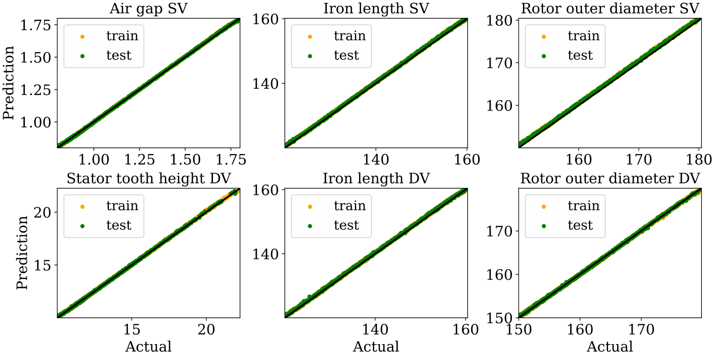
The mean absolute error (MAE), root mean squared error (RMSE), Pearson correlation coefficient (PCC), and dimensionless mean relative error (MRE) are used as quality metrics for KPIs prediction and parameter reconstruction. Figure 6 and Table I illustrates the predictions and evaluations for four KPIs over the test samples in the combined design space. Similarly, Table II and Table III provide evaluation details for important parameters of each topology. Prediction plots for three geometry parameters to each topology are demonstrated in Figure 7. The Figure 8 displays comparative evaluation of the prediction performance between MLP and VAE for each topology. The MLP for each topology is trained directly on the input parameters, as described in [1], using a supervised learning approach. The network configuration, training hyperparameters, and datasets (training, validation, and testing) are identical to the KPIs predictor for quantitative comparison. The VAE outperformed the MLP possibly due to a large number of training samples (through integrated parameter space) as compared to separately trained MLP for each topology, tuning of latent space dimension (slightly higher or the maximum number of topology parameters) that does better functional mapping between the latent input and output KPIs. The proposed method is applied for optimization based on the topologies. The trained MLP is used as a meta-model for the latent space.
Finally, in the latent space, two opposing objectives, maximum power and material cost, are optimized for demonstration. We use the multi-objective genetic algorithm NSGA-II [6]. The hyperparameter settings include sampling method (real random), random initialization, crossover, mutation, stopping criteria with maximum number of generations (100), population size (1000). The lower and upper bounds are determined using the mean values () of model training samples. In order to improve the design validation factor of the obtained designs in the pareto-front, the optimization process is constrained by the same bounds that were set during the data set generation. The optimization takes around hours. It can be seen from Figure 9 that the pareto-front consists of samples (unseen during model training) from each of the two topologies, which are cost-effective and/or power-efficient. Figure 1 depicts two samples (Design A and Design B) from the pareto-front. For reference, the result of a FE simulation is compared with the prediction in Table IV. The average MRE for KPIs prediction is less than for both samples.
V Conclusion
This paper presents a VAE-based approach to derive a unified parameterization for multiple PMSM topologies with different parameterizations and predicting KPIs with high accuracy simultaneously. It enables concurrent parametric optimization in multi-topology scenarios. The numerical results demonstrate that latent space optimization improves over the training data and produces novel (unseen in the training data) designs. The latent space dimension was observed to be a key hyperparameter for parameter reconstruction precision. This research lays the groundwork for parameter-based latent space optimization in the domain of the electric machines. A possible next step would be to investigate the impact of other latent space priors (e.g., Gaussian mixture models). It will also be interesting to extend the approach by involving different machine types (e.g., induction machines and flux switching machines).
References
- [1] V. Parekh, D. Flore, and S. Schöps, “Deep learning-based prediction of key performance indicators for electrical machines,” IEEE Access, vol. 9, pp. 21 786–21 797, 2021.
- [2] D. P. Kingma and M. Welling, “An introduction to variational autoencoders,” Foundations and Trends® in Machine Learning, vol. 12, no. 4, pp. 307–392, 2019.
- [3] Y. Pu, Z. Gan, R. Henao, X. Yuan, C. Li, A. Stevens, and L. Carin, “Variational autoencoder for deep learning of images, labels and captions,” in Advances in Neural Information Processing Systems, vol. 29. Curran Associates, Inc., 2016, pp. 2352–2360.
- [4] M. Tucci, S. Barmada, A. Formisano, and D. Thomopulos, “A regularized procedure to generate a deep learning model for topology optimization of electromagnetic devices,” Electronics, vol. 10, no. 18, 2021.
- [5] R. Gómez-Bombarelli, J. N. Wei, D. Duvenaud, J. M. Hernández-Lobato, B. Sánchez-Lengeling, D. Sheberla, J. Aguilera-Iparraguirre, T. D. Hirzel, R. P. Adams, and A. Aspuru-Guzik, “Automatic chemical design using a data-driven continuous representation of molecules,” ACS Central Science, vol. 4, no. 2, pp. 268–276, 2018.
- [6] K. Deb, A. Pratap, S. Agarwal, and T. Meyarivan, “A fast and elitist multiobjective genetic algorithm: NSGA-II,” IEEE Transactions on Evolutionary Computation, vol. 6, no. 2, pp. 182–197, 2002.
- [7] S. J. Salon, Finite Element Analysis of Electrical Machines. Kluwer, 1995.
- [8] D. P. Kingma and M. Welling, “Auto-encoding variational Bayes,” in International Conference on Learning Representations, 2014.
- [9] D. P. Kingma and J. L. Ba, “Adam: A method for stochastic optimization,” in International Conference on Learning Representations, 2015.