04CCS: Software and its engineering Software configuration management and version control systemsCCS: Software and its engineering Search-based software engineering

Md Shahriar Iqbal Affiliation: University of South Carolina email: miqbal@email.sc.edu , Rahul Krishna Affiliation: IBM Research email: rkrsn@ibm.com , Mohammad Ali Javidian Affiliation: Purdue University email: mjavidia@purdue.edu , Baishakhi Ray Affiliation: Columbia University email: rayb@cs.columbia.edu and Pooyan Jamshidi Affiliation: University of South Carolina email: pjamshid@cse.sc.edu

2022; © rightsretained

Abstract.

Modern computer systems are highly configurable, with the total variability space sometimes larger than the number of atoms in the universe. Understanding and reasoning about the performance behavior of highly configurable systems, over a vast and variable space, is challenging. State-of-the-art methods for performance modeling and analyses rely on predictive machine learning models, therefore, they become (i) unreliable in unseen environments (e.g., different hardware, workloads), and (ii) may produce incorrect explanations. To tackle this, we propose a new method, called Unicorn, which (i) captures intricate interactions between configuration options across the software-hardware stack and (ii) describes how such interactions can impact performance variations via causal inference. We evaluated Unicorn on six highly configurable systems, including three on-device machine learning systems, a video encoder, a database management system, and a data analytics pipeline. The experimental results indicate that Unicorn outperforms state-of-the-art performance debugging and optimization methods in finding effective repairs for performance faults and finding configurations with near-optimal performance. Further, unlike the existing methods, the learned causal performance models reliably predict performance for new environments.

Keywords:

Configurable Systems, Performance Modeling, Performance Debugging, Performance Optimization, Causal Inference, Counterfactual Reasoning

1. Introduction

(a)

(b)

(c)

Figure 1. An example showing the effectiveness of causality in reasoning about system performance behavior. (a) Observational data shows that the increase in Cache Misses leads to high Throughput and such trend is typically captured by statistical reasoning in ML models; (b) incorporating Cache Policy as a confounder correctly shows increase of Cache Misses corresponding to decrease in Throughput; (c) the corresponding causal model correctly captures Cache Policy as a common cause to explain performance behavior.

Modern computer systems, such as data analytics pipelines, are typically composed of multiple components, where each component has a plethora of configuration options that can be deployed individually or in conjunction with other components on different hardware platforms. The configuration space of such highly configurable systems is combinatorially large, with 100s if not 1000s of software and hardware configuration options that interact non-trivially with one another (wang2018understanding; halin2019test; JC:MASCOTS16; velez2022study). Individual component developers typically have a relatively localized, and thus limited, understanding of the performance behavior of the systems that comprise the components. Therefore, developers and end-users of the final system are often overwhelmed with the complexity of composing and configuring components, making it challenging and error-prone to configure these systems to reach desired performance goals.

Incorrect configuration (misconfiguration) elicits unexpected interactions between software and hardware, resulting in non-functional faults¹¹ 1 Non-functional and Performance faults are used interchangeably to refer to severe performance degradation caused by certain type of misconfigurations, (aka. specious configuration) (hu2020automated)., i.e., degradations in non-functional system properties like latency and energy consumption. These non-functional faults, unlike regular software bugs, do not cause the system to crash or exhibit any obvious misbehavior (reddy2016fault; tsakiltsidis2016automatic; nistor2013discovering). Instead, misconfigured systems remain operational but degrade in performance (bryant2003computer; molyneaux2009art; sanchez2020tandem; nistor2015caramel) that can cause major issues in cloud infrastructure (amazon:config:outage), internet-scale systems (fb:config:outage), and on-device machine learning (ML) systems (slowimag79:online). For example, a developer complained that “I have a complicated system composed of multiple components running on NVIDIA Nano and using several sensors and I observed several performance issues. (super_frustrated_power_perf:online).” In another instance, a developer asks “I’m quite upset with CPU usage on Jetson TX2 while running TCP/IP upload test program” (HighCPUu7:online). After struggling in fixing the issues over several days, the developer concludes, “there is a lot of knowledge required to optimize the network stack and measure CPU load correctly. I tried to play with every configuration option explained in the kernel documents.” In addition, they would like to understand the impact of configuration options and their interactions, e.g., “What is the effect of swap memory on increasing throughput? (slowimag79:online)”.

Existing works and gap. Understanding the performance behavior of configurable systems can enable (i) performance debugging (SGAK:ESECFSE15; GSKA:SPPEXA), (ii) performance tuning (H:CACM; SHM:LIO; H:AS; VPGFC:ICPE17; HPHL:ICSE15; WWHJK:GECCO15; NMSA:Arxive17; MARC:SPLC13; ORGC:SPLC14), and (iii) architecture adaptation (JGAP:CSMR13; ABDD:VISSOFT13; KK:WSR16; JVKSK:SEAMS17; HSCMAR:SIGPLAN; FHM:FSE15; EEM:TSE; EEM:FSE10). A common strategy is to build performance influence models such as regression models that explain the influence of individual options and their interactions (SGAK:ESECFSE15; VPGFC:ICPE17; GCASW:ASE13; pereira2019learning). These approaches are adept at inferring the correlations between configuration options and performance objectives, however, as illustrated in Figure 1 performance influence models suffer from several shortcomings (detailed in §2): (i) they become unreliable in unseen environments and (ii) produce incorrect explanations.

Our approach. Based on the several experimental pieces of evidence presented in the following sections, this paper proposes Unicorn–a methodology that enables reasoning about configurable system performance with causal inference and counterfactual reasoning. Unicorn first recovers the underlying causal structure from performance data. The causal performance model allows users to (i) identify the root causes of performance faults, (ii) estimate the causal effects of various configurable parameters on the performance objectives, and (iii) prescribe candidate configurations to fix the performance fault or optimize system performance.

Refer to caption — Figure 2. Deepstream: An example of a highly-configurable composed system, a big data analytics pipeline system, with several configurable components: (i) Video Decoder performs video encoding/decoding with different formats; (ii) Stream Muxer accepts input streams and converts them to sequential batch frames; (iii) Primary Detector transforms the input frames based on input NN requirements and makes model inference to detect objects; (iv) Object Tracker supports multi-object tracking; (v) Secondary Classifier improves performance by avoiding re-inferencing.

Contributions. Our contributions are as follows:

•

We propose Unicorn (§4), a novel approach that allows causal reasoning about system performance.
•

We have conducted a thorough evaluation of Unicorn in a controlled case study (§5) as well as real-world large-scale experiments. In particular, we evaluated effectiveness (§7), transferability (§8), and scalability (§9) by comparing Unicorn with: (i) state-of-the-art performance debugging approaches, including CBI (song2014statistical), DD (artho2011iterative), EnCore (zhang2014encore), and BugDoc (lourencco2020bugdoc) and (ii) performance optimization techniques, including SMAC (hutter2011sequential) and PESMO (hernandez2016predictive). The evaluations were conducted on six real-world highly configurable systems, including a video analytic pipeline, Deepstream (DeepStream), three deep learning-based systems, Xception (chollet2017xception), Deepspeech (hannun2014deep), and BERT (devlin2018bert), a video encoder, X264 (x264), and a database engine, SQLite (SQLite), deployed on NVIDIA Jetson hardware (TX1, TX2, and Xavier).
•

In addition to sample efficiency and accuracy of Unicorn in finding root causes of performance issues, we show that the learned causal performance model is transferable across different workload and deployment environments. Finally, we demonstrate the scalability of Unicorn to large systems consisting of 500 options and several trillion potential configurations.
•

The artifacts and supplementary materials can be found at https://github.com/softsys4ai/unicorn.

2. Motivating Scenarios

(a) Performance Distribution

Config. Option Value CPU Cores 2 CPU Frequency (GHz) 0.1 EMC Frequency (GHz) 1.6 GPU Frequency (GHz) 0.7 Scheduler Policy noop Scheduler Runtime ( $\mu$ s) 950k Scheduler Child Runs First 1 Batched Push Timeout 1 Batch Size 1 Interval 1 Buffer Size 6000 Dirty Background Ratio 5 Dirty Ratio 10 Drop Caches 0 Cache Pressure 500 Swappiness 60 Enable Padding 1 Offset 0 Swap Memory (Gb) 1 Sched Time Avg (ms) 1000 Dirty Bytes 30 Overcommit Memory 2 Overcommit Hugepages 1 Throughput (FPS) 6.8 Energy (J) 122

(b) Misconfiguration

Figure 3. (a) Performance distribution when Deepstream is deployed on NVIDIA Jetson Xavier (b) Misconfiguration that caused the multi-objective non-functional fault, shown as

\square

in the performance distribution.

Simple motivating scenario. In this simple scenario, we motivate our work by demonstrating why performance analyses solely based on correlational statistics may lead to an incorrect outcome. Here, the collected performance data indicates that Throughput is positively correlated with increased Cache Misses²² 2 we used a distinct font to indicate variables such as configuration options or performance metrics and events throughout this paper. (as in Figure 1 (a)). A simple ML model built on this data will predict with high confidence that larger Cache Misses leads to higher Throughput—this is misleading as higher Cache Misses should, in theory, lower Throughput. By further investigating the performance data, we noticed that the caching policy was automatically changed during measurement. We then segregated the same data on Cache Policy (as in Figure 1 (b)) and found out that within each group of Cache Misses, as Cache Misses increases, the Throughput decreases. One would expect such behavior, as the more Cache Misses the higher number of access to external memory, and, therefore, the Throughput would be expected to decrease. The system resource manager may change the Cache Policy based on some criteria; this means that for the same number of Cache Misses, the Throughput may be lower or higher; however, in all Cache Policies, the increases of Cache Misses resulting in a decrease in Throughput. Thus, Cache Policy acts as a confounder that explains the relation between Cache Misses and Throughout, which a correlation-based model will not be able to capture. In contrast, a causal performance model, as shown in Figure 1 (c), finds the relation between Cache Misses, Cache Policy, and Throughput and thus can reason about the observed behavior correctly.

In reality, performance analysis and debugging of heterogeneous multi-component systems is non-trivial and often compared with finding the needle in the haystack (whitaker2004configuration). In particular, the end-to-end performance analysis is not possible by reasoning about individual components in isolation, as components may interact with one another in such a composed system. Below, we use a highly configurable multi-stack system to motivate why causal reasoning is a better choice for understanding the performance behavior of complex systems.

Motivating scenario based on a highly configurable data analytics system. We deployed a data analytics pipeline, Deepstream (DeepStream). Deepstream has many components, and each component has many configuration options, resulting in several variants of the same system as shown in Figure 2. Specifically, the variability arises from: (i) the configuration options of each software component in the pipeline, (ii) configurable low-level libraries that implement functionalities required by different components (e.g., the choice of tracking algorithm in the tracker or different neural network architectures), (iii) the configuration options associated with each component’s deployment stack (e.g., CPU Frequency of Xavier). Further, there exist many configurable events that can be measured/observed at the OS level by the event tracing system. More specifically, the configuration space of the system includes (i) 27 Software options (Decoder: 6, Stream Muxer: 7, Detector: 10, Tracker: 4), (ii) 22 Kernel options (e.g., Swappiness, Scheduler Policy, etc.), and (iii) 4 Hardware options (CPU Frequency, CPU Cores, etc.). We use 8 camera streams as the workload, x264 as the decoder, TrafficCamNet model that uses ResNet 18 architecture for the detector, and an NvDCF tracker, which uses a correlation filter-based online discriminative learning algorithm for tracking. Such a large space of variability makes performance analysis challenging. This is further exacerbated by the fact that the configuration options among the components interact with each other. Additional details about our Deepstream implementation can be found in the supplementary materials.

To better understand the potential of the proposed approach, we measured (i) application performance metrics including throughput and energy consumption by instrumenting the Deepstream code, and (ii) 288 system-wide performance events (hardware, software, cache, and tracepoint) using $perf$ and measured performance for 2461 configurations of Deepstream in two different hardware environments, Xavier, and TX2. As it is depicted in Figure 3a, performance behavior of Deepstream, like other highly configurable systems, is non-linear, multi-modal, and non-convex (jamshidi2016uncertainty). In this work, we focus on two performance tasks: (i) Performance Debugging: here, one observes a performance issue (e.g., latency), and the task involves replacing the current configurations in the deployed environment with another that fixes the observed performance issue; (ii) Performance Optimization: here, no performance issue is observed; however, one wants to get a near-optimal performance by finding a configuration that enables the best trade-off in the multi-objective space (e.g., throughput vs. energy consumption vs. accuracy in Deepstream).

To show major shortcomings of existing state-of-the-art performance models, we built performance influence models that have extensively been used in the systems’ literature (siegmund2015performance; JSVKPA:ASE17; GCASW:ASE13; GSKA:SPPEXA; kolesnikov2019tradeoffs; kaltenecker2020interplay; muhlbauer2019accurate; grebhahn2019predicting; siegmund2020dimensions) and it is the standard approach in industry (kolesnikov2019tradeoffs; kaltenecker2020interplay). Specifically, we built non-linear regression models with forward and backward elimination using a step-wise training method on the Deepstream performance data. We then performed several sensitivity analyses and identified the following issues:

(1)

Performance influence models could not reliably predict performance in unseen environments. Performance behavior of configurable systems vary across environments, e.g., when we deploy software on new hardware with a different microarchitecture or when the workload changes (JSVKPA:ASE17; JVKSK:SEAMS17; JVKS:FSE18; iqbal_transfer_2019; VPGFC:ICPE17). When building a performance model, it is important to capture predictors that transfer well, i.e., remain stable across environmental changes. The predictors in performance models are options ( $o_{i}$ ) and interactions ( $\phi(o_{i}..o_{j})$ ) that appear in the explainable models of form $f(c)=\beta_{0}+\Sigma_{i}{\phi(o_{i})}+\Sigma_{i..j}{\phi(o_{i}..o_{j})}$ . The transferability of performance predictors is expected from performance models since they are learned based on one environment (e.g., staging as the source environment) and are desirable to reliably predict performance in another environment (e.g., production as the target environment). Therefore, if the predictors in a performance model become unstable, even if they produce accurate predictions in the current environment, there is no guarantee that it performs well in other environments, i.e., they become unreliable for performance predictions and performance optimizations due to large prediction errors. To investigate how transferable performance influence models are across environments, we performed a thorough analysis when learning a performance model for DeepStream deployed on two different hardware platforms that have two different microarchitectures. Note that such environmental changes are common, and it is known that performance behavior changes when, in addition to a change in hardware resources (e.g., higher CPU Frequency), we have major differences in terms of architectural constructs (ding2021generalizable; curtsinger2013stabilizer), also supported by a thorough empirical study (JSVKPA:ASE17). The results in Figure 4 (a) indicate that the number of stable predictors is too small for the total number of predictors that appear in the learned regression models. Additionally, the coefficients of the common predictors change across environments as shown in Figure 5 making them unreliable to be resued in the new scenario.
(2)

Performance influence models could produce incorrect explanations. In addition to performance predictions, where developers are interested to know the effect of configuration changes on performance objectives, they are also interested to estimate and explain the effect of a change in particular configuration options (e.g., changing Cache Policy) toward performance variations. It is therefore desirable that the strength of the predictors in performance models, determined by their coefficients, remain consistent across environments (ding2021generalizable; JSVKPA:ASE17). In the context of our simple scenario in Figure 1, the learned performance influence model indicates that $0.16\times\texttt{Cache Misses}$ is the most influential term that determines throughput, however, the (causal) model in Figure 1 (c) show that the interactions between configuration option Cache Policy and system event Cache Misses is a more reliable predictor of the throughput, indicating that the performance influence model, due to relying on superficial correlational statistics, incorrectly explains factors that influence performance behavior of the system. The low Spearman rank correlation between predictors coefficients indicates that a performance model based on regression could be highly unstable and thus would produce unreliable explanations as well as unreliable estimation of the effect of change in specific options for performance debugging or optimization.

Figure 4. (a) Performance influence models do not generalize well as the number of common terms, total terms and prediction error of these models change from source (Xavier) to target (TX2). The rank correlation between source and target is 0.07 (p-value=0.73). (b) Causal performance models generalize better as the number of common terms, total terms and prediction error of the structural does not change much from source (Xavier) to target (TX2). The rank correlation between source and target is 0.49 (p-value=0.76).

Figure 5. Visualizing co-efficient differences from the source (Xavier) performance influence model to the target (TX2) performance influence model for the common terms for both options and interactions (shown by

\otimes

3. Causal Reasoning for Systems

We hypothesize that the reason behind unreliable predictions and incorrect explanations of performance influence models (see §3) is the inability of correlation-based models to capture causally relevant predictors in the learned performance models. The theoretical and empirical results (JSVKPA:ASE17; javidian2019transfer) also show that predictive models that contain non-causal predictors, even though they might be accurate in the environment that the training data come from, such models are not typically transferable in unseen environments.

Hence, we introduce a new abstraction for performance modeling, called Causal Performance Model, which gives us the leverage for performing causal reasoning for computer systems. In particular, we introduce the causal performance model to serve as a modeling abstraction that allow building reusable performance models for downstream performance tasks, including performance predictions, performance testing and debugging, performance optimization, and more importantly, it serves as a transferable model that allow performance analyses across environments (JSVKPA:ASE17; javidian2019transfer).

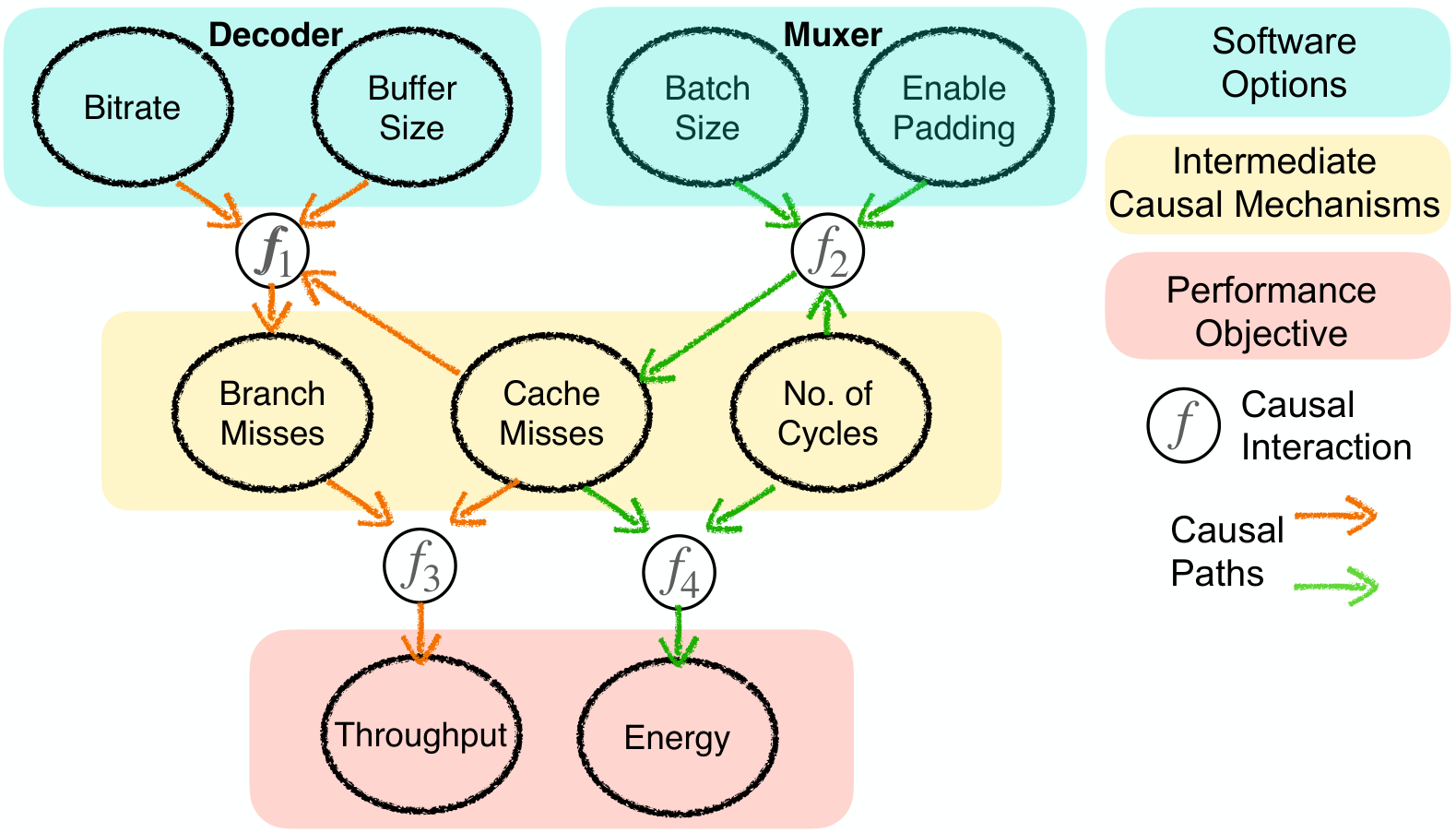
Causal performance models. We define a causal performance model as an instantiation of Probabilistic Graphical Models (pearl1998graphical) with new types and structural constraints to enable performance modeling and analyses. Formally, causal performance models (cf., Figure 6) are Directed Acyclic Graphs (DAGs) (pearl1998graphical) with (i) performance variables, (ii) functional nodes that define functional dependencies between performance variables (i.e., how variations in one or multiple variables determine variations in other variables), (iii) causal links that interconnect performance nodes with each other via functional nodes, and (iv) constraints to define assumptions we require in performance modeling (e.g., software configuration options cannot be the child node of performance objectives; or Cache Misses as a performance variable takes only positive integer values). In particular, we define three new variable types: (i) Software-level configuration options associated with a software component in the composed system (e.g., Bitrate in the decoder component of Deepstream), and hardware-level options (e.g., CPU Frequency), (ii) intermediate performance variables relating the effect of configuration options to performance objectives including middleware traces (e.g., Context Switches), performance events (e.g., Cache Misses) and (iii) end-to-end performance objectives (e.g., Throughput). In this paper, we characterize the functional nodes with polynomial models, because of their simplicity and their explainable nature, however, they could be characterized with any functional forms, e.g., neural networks (xia2021causal; scherrer2021learning). We also define two specific constraints over causal performance models to characterize the assumptions in performance modeling: (i) defining variables that can be intervened (note that some performance variables can only be observed (e.g., Cache Misses) or in some cases where a variable can be intervened, the user may want to restrict the variability space, e.g., the cases where the user may want to use prior experience, restricting the variables that do not have a major impact to performance objectives); (ii) structural constraints, e.g., configuration options do not cause other options. Note that such constraints enable incorporating domain knowledge and enable further sparsity that facilitates learning with low sample sizes.

How causal reasoning can fix the reliability and explainability issues in current performance analyses practices?. The causal performance models contain more detail than the joint distribution of all variables in the model. For example, the causal performance model in Figure 6 encodes not only Branch Misses and Throughput readings are dependent but also that lowering Cache Misses causes the Throughput of Deepstream to increase and not the other way around. The arrows in causal performance models correspond to the assumed direction of causation, and the absence of an arrow represents the absence of direct causal influence between variables, including configuration options, system events, and performance objectives. The only way we can make predictions about how performance distribution changes for a system when deployed in another environment or when its workload changes are if we know how the variables are causally related. This information about causal relationships is not captured in non-causal models, such as regression-based models. Using the encoded information in causal performance models, we can benefit from analyses that are only possible when we explicitly employ causal models, in particular, interventional and counterfactual analyses (pearl2009causality; pearl2018book). For example, imagine that in a hardware platform, we deploy the Deepstream and observed that the system throughput is below 30 FPS and Buffer Size as one of the configuration options was determined dynamically between 8k-20k. The system maintainers may be interested in estimating the likelihood of fixing the performance issue in a counterfactual world where the Buffer Size is set to a fixed value, 6k. The estimation of this counterfactual query is only possible if we have access to the underlying causal model because setting a specific option to a fixed value is an intervention as opposed to conditional observations that have been done in the traditional performance model for performance predictions.

Causal performance models are not only capable of predicting system performance in certain environments, they encode the causal structure of the underlying system performance behavior, i.e., the data-generating mechanism behind system performance. Therefore, the causal model can reliably transfer across environments (scholkopf2021toward). To demonstrate this for causal performance models as a particular characterization of causal models, we performed a similar sensitivity analysis to regression-based models and observed that causal performance models can reliably predict performance in unseen environments (see Figure 4 (b)). In addition, as opposed to performance influence models that are only capable of performance predictions, causal performance models can be used for several downstream heterogeneous performance tasks. For example, using a causal performance model, we can determine the causal effects of configuration options on performance objectives. Using the estimated causal effects, one can determine the effect of change in a particular set of options towards performance objectives and therefore can select the options with the highest effects to fix a performance issue, i.e., bring back the performance objective that has violated a specific quality of service constraint without sacrificing other objectives. Causal performance models are also capable of predicting performance behavior by calculating conditional expectation, $E(Y|X)$ , where $Y$ indicates performance objectives, e.g., throughput, and $X=x$ is the system configurations that have not been measured.

4. Unicorn

This section presents Unicorn–our methodology for performance analyses of highly configurable and composable systems with causal reasoning.

Overview.

Unicorn works in five stages, implementing an active learning loop (cf. Figure 7): (i) Users or developers of a highly-configurable system specify, in a human-readable language, the performance task at hand in terms of a query in the Inference Engine. For example, a Deepstream user may have experienced a throughput drop when they have deployed it on NVIDIA Xavier in low-power mode (cf. Figure 8). Then, Unicorn’s main process starts by (ii) collecting some predetermined number of samples and learning a causal performance model; Here, a sample contains a system configuration and its corresponding measurement—including low-level system events and end-to-end system performance. Given a certain budget, which in practice either translates to time (iqbal2020flexibo) or several samples (jamshidi2016uncertainty), Unicorn, at each iteration, (iii) determines the next configuration(s) and measures system performance when deployed with the determined configuration–i.e. new sample; accordingly, (iv) the learned causal performance model is incrementally updated, reflecting a model that captures the underlying causal structure of the system performance. Unicorn terminates if either budget is exhausted or the same configuration has been selected a certain number of times consecutively, otherwise, it continues from Stage III. Finally, (v) to automatically derive the quantities which are needed to conduct the performance tasks, the specified performance queries are translated to formal causal queries, and they will be estimated based on the final causal model.

Stage I: Formulate Performance Queries.

Unicorn enables developers and users of highly-configurable systems to conduct performance tasks, including performance debugging, optimization, and tuning, n particular, when they need to answer several performance queries: (i) What configuration options caused the performance fault? (ii) What are important options and their interactions that influence performance? (iii) How to optimize one quality or navigate tradeoffs among multiple qualities in a reliable and explainable fashion? (iv) How can we understand what options and possible interactions are most responsible for the performance degradation in production?

At this stage, the performance queries are translated to formal causal queries using the interface of the causal inference engine (cf. Figure 7). Note that in the current implementation of Unicorn, this translation is performed manually, however, this process could be made automated by creating a grammar for specifying performance queries and the translations can be made between the performance queries into the well-defined causal queries, note that such translation has been done in domains such as genomics (farahmand2019causal).

Stage II: Learn Causal Performance Model.

In this stage, Unicorn learns a causal performance model (see Section 2) that explains the causal relations between configuration options, the intermediate causal mechanism, and performance objectives. Here, we use an existing structure learning algorithm called Fast Causal Inference (hereafter, FCI) (spirtes2000causation). We selected FCI because: (i) it accommodates for the existence of unobserved confounders (spirtes2000causation; ogarrio2016hybrid; glymour2019review), i.e., it operates even when there are latent common causes that have not been, or cannot be, measured. This is important because we do not assume absolute knowledge about configuration space, hence there could be certain configurations we could not modify or system events we have not observed. (ii) FCI, also, accommodates variables that belong to various data types such as nominal, ordinal, and categorical data common across the system stack (cf. Figure 8). To build the causal performance model, we, first, gather a set of initial samples (cf. Figure 9). To ensure reliability (curtsinger2013stabilizer; ding2021generalizable), we measure each configuration multiple times, and we use the median (as an unbiased measure) for the causal model learning. As depicted in Figure 9, Unicorn implements three steps for causal structure learning: (i) recovering the skeleton of the causal performance model by enforcing structural constraints; (ii) pruning the recovered structure using standard statistical tests of independence. In particular, we use mutual info for discrete variables and Fisher z-test for continuous variables; (iii) orienting undirected edges using entropy (spirtes2000causation; ogarrio2016hybrid; glymour2019review; colombo2012learning; colombo2014order).

Orienting undirected causal links. We orient undirected edges using prescribed edge orientation rules (spirtes2000causation; ogarrio2016hybrid; glymour2019review; colombo2012learning; colombo2014order) to produce a partial ancestral graph (or PAG). A PAG contains the following types of (partially) directed edges:

•

$X$ $Y$ indicating that vertex $X$ causes $Y$ .
•

$X$ $Y$ which indicates that there are unmeasured confounders between vertices $X$ and $Y$ .

In addition, a PAG produces two types of edges:

•

$X$ $Y$ indicating that either $X$ causes $Y$ , or that there are unmeasured confounders that cause both $X$ and $Y$ .
•

$X$ $Y$ which indicates that either: (a) vertices $X$ causes $Y$ , or (b) vertex $Y$ causes $X$ , or (c) there are unmeasured confounders that cause both $X$ and $Y$ .

Figure 11. (a) The hamming distance between the learned causal model and ground truth model decreases as the algorithms measure more configuration samples. Incremental update of (b) Latency and (c) Energy, using Unicorn for debugging a multi-objective fault. Configuration options selected by Unicorn at each iteration are during debugging are shown in (d) using the yellow-colored nodes. Red-colored nodes indicate configuration options that are selected as a fix to the multi-objective performance fault. Mapping between option indexes and configuration options are shown in the supplementary materials.

In the last two cases, the circle ( $\circ$ ) indicates that there is an ambiguity in the edge type. In other words, given the current observational data, the circle can indicate an arrowhead ( ) or no arrowhead (—), i.e., for $X$ $Y$ , all three of $X$ $Y$ , $Y$ $X$ , and $X$ $Y$ might be compatible with current data, i.e., the current data could be faithful to each of these statistically equivalent causal graphs inducing the same conditional independence relationships.

Resolving partially directed edges. For subsequent analyses over the causal graph, the PAG obtained must be fully resolved (directed with no $\circ$ ended edges) in order to generate an ADMG. We use the information-theoretic approach using entropy proposed in (Kocaoglu2017; Kocaoglu2020) to discover the true causal direction between two variables. Our work extends the theoretic underpinnings of entropic causal discovery to generate a fully directed causal graph by resolving the partially directed edges produced by FCI. For each partially directed edge, we follow two steps: (i) establish if we can generate a latent variable (with low entropy) to serve as a common cause between two vertices; (ii) if such a latent variable does not exist, then pick the direction which has the lowest entropy.

For the first step, we assess if there could be an unmeasured confounder (say $Z$ ) that lies between two partially oriented nodes (say $X$ and $Y$ ). For this, we use the LatentSearch algorithm proposed by Kocaoglu et al. (Kocaoglu2020). LatentSearch outputs a joint distribution $q(X,Y,Z)$ of the variables $X$ , $Y$ , and $Z$ which can be used to compute the entropy $H(Z)$ of the unmeasured confounder $Z$ . Following the guidelines of Kocaoglu et al., we set an entropy threshold $\theta_{r}=0.8\times min\left\{H(X),H(Y)\right\}$ . If the entropy $H(Z)$ of the unmeasured confounder falls below this threshold, then we declare that there is a simple unmeasured confounder $Z$ (with a low enough entropy) to serve as a common cause between $X$ and $Y$ and accordingly, we replace the partial edge with a bidirected (i.e., ) edge.

When there is no latent variable with a sufficiently low entropy, two possibilities exist: (i) variable $X$ causes $Y$ ; then, there is an arbitrary function $f(\cdot)$ such that $Y=f(X,E)$ , where $E$ is an exogenous variable (independent of $X$ ) that accounts for system noise; or (ii) variable $Y$ causes $X$ ; then, there is an arbitrary function $g(\cdot)$ such that $X=g(Y,\tilde{E})$ , where $\tilde{E}$ is an exogenous variable (independent of $Y$ ) that accounts for noise in the system. The distribution of $E$ and $\tilde{E}$ can be inferred from the data (Kocaoglu2017, see §3.1). With these distributions, we measure the entropies $H(E)$ and $H(\tilde{E})$ . If $H(E)<H(\tilde{E})$ , then, it is simpler to explain the $X$ $Y$ (i.e., the entropy is lower when $Y=f(X,E)$ ) and we choose $X$ $Y$ . Otherwise, we choose $Y$ $X$ .

Problem (code_transplant:online): For a real-time scene detection task, TX2 (faster platform) only processed 4 frames/sec whereas TX1 (slower platform) processed 17 frames/sec, i.e., the latency is

4\times

worse on TX2.

Observed Latency (frames/sec): 4 FPS

Expected Latency (frames/sec): 22-24 FPS (30-40% better)


Configuration Options	Unicorn	SMAC	BugDoc	Forum	ACE^†

CPU Cores					3%
CPU Frequency					6%
EMC Frequency					13%
GPU Frequency					22%
Scheduler Policy	$\cdot$			$\cdot$	.
kernel.sched_rt_runtime_us	$\cdot$	$\cdot$		$\cdot$	.
kernel.sched_child_runs_first	$\cdot$	$\cdot$		$\cdot$	.
vm.dirty_background_ratio	$\cdot$	$\cdot$	$\cdot$	$\cdot$	.
vm.dirty_ratio	$\cdot$	$\cdot$		$\cdot$	.
Drop Caches	$\cdot$			$\cdot$	.
CUDA_STATIC					55%
vm.vfs_cache_pressure	$\cdot$	$\cdot$	$\cdot$	$\cdot$	.
vm.swappiness	$\cdot$			$\cdot$	1%


Latency (TX2 frames/sec)	28	24	21	23
Latency Gain (over TX1)	65%	41%	24%	35%
Latency Gain (over default)	7 $\times$	6 $\times$	5.25 $\times$	5.75 $\times$
Resolution time	22 mins	4 hrs	4 hrs	2 days

Figure 12. Using Unicorn on a real-world performance issue.

Stage III: Iterative Sampling (Active Learning).

At this stage, Unicorn determines the next configuration to be measured. Unicorn first estimates the causal effects of configuration options towards performance objectives using the learned causal performance model. Then, Unicorn iteratively determines the next system configuration using the estimated causal effects as a heuristic. Specifically, Unicorn determines the value assignments for options with a probability that is determined proportionally based on their associated causal effects. The key intuition is that such changes in the options are more likely to have a larger effect on performance objectives, and therefore, we can learn more about the performance behavior of the system. Given the exponentially large configuration space and the fact that the span of performance variations is determined by a small percentage of configurations, if we had ignored such estimates for determining the change in configuration options, the next configurations would result in considerable variations in performance objectives comparing with the existing data. Therefore, measuring the next configuration would not provide additional information for the causal model.

We extract paths from the causal graph (referred to as causal paths) and rank them from highest to lowest based on their average causal effect on latency, and energy. Using path extraction and ranking, we reduce the complex causal graph into a few useful causal paths for further analyses. The configurations in this path are more likely to be associated with the root cause of the fault.

Extracting causal paths with backtracking. A causal path is a directed path originating from either the configuration options or the system event and terminating at a non-functional property (i.e., throughput and/or energy). To discover causal paths, we backtrack from the nodes corresponding to each non-functional property until we reach a node with no parents. If any intermediate node has more than one parent, then we create a path for each parent and continue backtracking on each parent.

Ranking causal paths. A complex causal graph can result in many causal paths. It is not practical to reason over all possible paths, as it may lead to a combinatorial explosion. Therefore, we rank the paths in descending of their causal effect on each non-functional property. For further analysis, we use paths with the highest causal effect. To rank the paths, we measure the causal effect of changing the value of one node (say Batch Size or $X$ ) on its successor (say Cache Misses or $Z$ ) in the path (say Batch Size Cache Misses FPS and Energy). We express this with the do-calculus (pearl2009causality) notation: $\mathbb{E}[Z~|~\mathit{do}(X=x)]$ . This notation represents the expected value of $Z$ (Cache Misses) if we set the value of the node $X$ (Batch Size) to $x$ . To compute the average causal effect (ACE) of $X\rightarrow Z$ (i.e., Batch Size Cache Misses), we find the average effect over all permissible values of $X$ (Batch Size), i.e., $\mathrm{ACE}\left(Z,X\right)=\frac{1}{N}\cdot\sum_{\forall a,b\in X}\mathbb{E}\left[Z~|~\mathit{do}\left(X=b\right)\right]~-~\mathbb{E}\left[Z~|~\mathit{do}\left(X=a\right)\right]$ . Here $N$ represents the total number of values $X$ (Batch Size) can take. If changes in Batch Size result in a large change in Cache Misses, then $\mathrm{ACE}\left(Z,X\right)$ will be larger, indicating that Batch Size has a large causal effect on Cache Misses.

Stage IV: Update Causal Performance Model.

At each iteration, Unicorn measures the configuration that is determined in the previous stage and updates the causal performance model incrementally (shown in Figure 10). Since the causal model uses limited observational data, there may be a discrepancy between the underlying performance model and the learned causal performance model, note that this issue exists in all domains using data-driven models, including causal reasoning (pearl2009causality). The more accurate the causal graph, the more accurate the proposed intervention will be (spirtes2000causation; ogarrio2016hybrid; glymour2019review; colombo2012learning; colombo2014order). Figure 11 (a) shows an example of an iterative decrease of hamming distance (norouzi2012hamming) between the learned causal model and (approximate) ground truth causal model. Figure 11 (b), 11 (c), and 11 (d) shows the iterative behavior of Unicorn while debugging a multi-objective performance fault. In case our repairs do not fix the faults, we update the observational data with this new configuration and repeat the process. Over time, the estimations of causal effects will become more accurate. We terminate the incremental learning once we achieve the desired performance.

Stage V: Estimate Performance Queries.

At this stage, given the learned causal performance model, Unicorn’s inference engine estimates the user-specified queries using the mathematics of causal reasoning–do-calculus. Specifically, the causal inference engine provides a quantitative estimate for the identifiable queries on the current causal model and may return some queries as unidentifiable. It also determines what assumptions or new measurements are required to answer the “unanswerable“ questions, so, the user can decide to incorporate these new assumptions by defining more constraints or increasing the sampling budgets.

5. Case Study

Figure 13. Distribution of 451 single-objective and 43 multi-objective non-functional faults across different software systems used in our study.

Prior to a systematic evaluation in §6, here, we show how Unicorn can enable performance debugging in a real-world scenario discussed in (code_transplant:online), where a developer migrated a real-time scene detection system from NVIDIA TX1 to a more powerful hardware, TX2. The developer, surprisingly, experienced $4\times$ worse latency in the new environment (from 17 frames/sec in TX1 to 4 frames/sec in TX2). After two days of discussions, the performance issue was diagnosed with a misconfiguration–an incorrect setting of a compiler option and four hardware options. Here, we assess whether and how Unicorn could facilitate the performance debugging by comparing with (i) the fix suggested by NVIDIA in the forum, and two academic performance debugging approaches–BugDoc (lourencco2020bugdoc) and SMAC (hutter2011sequential).

Findings. Figure 12 illustrates our findings. We find that:

•

Unicorn could diagnose the root cause of the misconfiguration and recommends a fix within 22 minutes. Using the recommended configuration from Unicorn, we achieved a throughput of 28 frames/sec ( $65\%$ higher than TX1 and $7\times$ higher than the fault). This, surprisingly, exceeds the developers’ initial expectation of $30-40\%$ improvement.
•

BugDoc (a diagnosis approach) has the least improvement compared to other approaches ( $24\%$ improvement over TX1) while taking 4 hours to suggest the fix. BugDoc also changed several unrelated options (depicted by ) not endorsed by the domain experts.
•

Using SMAC (an optimization approach), we aimed to find a configuration that achieves optimal throughput. However, after converging, SMAC recommended a configuration which achieved 24 frames/sec ( $41\%$ better than TX1 and $6\times$ better than the fault), however, could not outperform the configuration suggested by Unicorn and even took 4 hours ( $11\times$ longer than Unicorn to converge). In addition, SMAC changed several unrelated options ( in Figure 12).

Why Unicorn works better (and faster)? Unicorn discovers the misconfigurations by constructing a causal model that rules out irrelevant configuration options and focuses on the configurations that have the highest (direct or indirect) causal effect on latency, e.g., we found the root-cause CUDA STATIC in the causal graph which indirectly affects latency via Context Switches (an intermediate system event). Using counterfactual queries, Unicorn can reason about changes to configurations with the highest average causal effect (ACE) (last column in Figure 12). The counterfactual reasoning occurs no additional measurements, significantly speeding up inference as shown in Figure 12, Unicorn accurately finds all the configuration options recommended by the forum (depicted by in Figure 12).

6. Evaluation

Table 1. Overview of the subject systems used in our study. Details about the configuration options and system events for each system are found in the supplementary materials.

System	Workload	$\|\mathcal{C}\|$	$\|\mathcal{O}\|$	$\|\mathcal{S}\|$	$\|\mathcal{H}\|$	$\|\mathcal{W}\|$	$\|\mathcal{P}\|$
Deepstream (DeepStream)	Video analytics pipeline for detection and tracking from 8 camera streams.	2461	53	288	2	1	2
Xception (chollet2017xception)	Image recognition system to classify 5000/5000 test images from CIFAR10.	6443	28	19	3	3	3
Deepspeech (hannun2014deep)	Speech-to-text from 0.5/1932 hours of Common Voice Corpus 5.1 (English) data.	6112	28	19	3	1	3
Bert (devlin2018bert)	NLP system for sentiment analysis of 1000/25000 test reviews from IMDb.	6188	28	19	3	1	3
x264 (x264)	Encodes a 20 second 11.2 MB video of resolution 1920 x 1080 from UGC.	17248	32	19	3	1	3
SQLite (SQLite)	Database engine for sequential & batch & random reads, writes, deletions.	15680	242	288	3	3	3

* $\mathcal{C}$ : Configurations, $\mathcal{O}$ : Options, $\mathcal{S}$ : System Events, $\mathcal{H}$ : Hardware, $\mathcal{W}$ : Workload, $\mathcal{P}$ : Objectives

For a thorough evaluation of Unicorn, we have developed $\textsc{Unicorn}_{\textsc{Tool}}$ that implements the methodology that we explained in §4. We used $\textsc{Unicorn}_{\textsc{Tool}}$ (see §A) to facilitate comparing Unicorn with state-of-the-art performance debugging and optimization approaches for:

•

Effectiveness in terms of sample efficiency and performance gain (§7).
•

Transferability of learned models across environmental changes such as hardware and workload changes (§8).
•

Scalability to large-scale configurable systems (§9).

Systems. We selected six configurable systems including a video analytic pipeline, three deep learning-based systems (for image, speech, and NLP), a video encoder, and a database, see Table 1. We use heterogeneous deployment platforms, including NVIDIA TX1, TX2, and Xavier, each having different resources (compute, memory) and microarchitectures.

Configurations. We choose a wide range of configuration options and system events (see Table 1), following NVIDIA’s configuration guides/tutorials and other related work (Halawa2017). As opposed to prior works (e.g., (velez2021white; VJSSAK:ASE20)) that only support binary options due to scalability issues, we included options with binary, discrete, and continuous.

Ground truth. We measured several thousands samples (proportional to the configuration space of the system, see supplementary materials for specific dataset size) for each 18 deployment settings (6 systems and 3 hardware; see Table 1 for more details). To ensure reliable and replicable results, following the common practice (ding2021generalizable; JSVKPA:ASE17; curtsinger2013stabilizer; kaltenecker2020interplay), we repeated each measurement $5$ times and used the median in the evaluation metrics. We curated a ground truth of performance issues, called Jetson Faults, for each of the studied software and hardware systems using the ground truth data. By definition, non-functional faults are located in the tail of performance distributions (gunawi2018fail; kleppmann2017designing). We, therefore, selected and labeled configurations that are worse than the $99^{\text{th}}$ percentile as ‘faulty.’ Figure 13 shows the total 494 faults discovered across different software. Out of these 494 non-functional faults, 43 are faults with multiple types (both energy and latency). Of all the 451 single-objective and 43 multi-objective faults discovered in this study, only 2 faults had a single root cause, 411 faults had five or more root causes, and 81 remaining faults had two to four root causes.

Experimental parameters. To facilitate replication of the results, we made some choices for specific parameters. In particular, we disabled dynamic voltage and frequency scaling (DVFS) before starting any experiment and start with 25 samples for each method (10% of the total sampling budget). We repeat the entire process 3 times for consistent analyses.

Table 2. Efficiency of Unicorn compared to other approaches. Cells highlighted in blue indicate improvement over faults.


			Accuracy					Precision					Recall					Gain					Time^†

			Unicorn	CBI	DD	EnCore	BugDoc	Unicorn	CBI	DD	EnCore	BugDoc	Unicorn	CBI	DD	EnCore	BugDoc	Unicorn	CBI	DD	EnCore	BugDoc	Unicorn	Others

		DeepStream	87	61	62	65	81	83	66	59	60	71	80	61	65	60	70	88	66	67	68	79	0.8	4
		Xception	86	53	42	62	65	86	67	61	63	67	83	64	68	69	62	82	48	42	57	59	0.6	4
		BERT	81	56	59	60	57	76	57	55	61	73	71	74	68	67	65	74	54	59	62	58	0.4	4
		Deepspeech	81	61	59	60	72	76	58	69	61	71	81	73	61	63	69	76	59	53	55	66	0.7	4
TX2	Latency	x264	83	59	63	62	62	82	69	58	65	66	78	64	67	63	72	85	69	72	68	71	1.4	4

		DeepStream	91	81	79	77	87	81	61	62	64	73	85	63	61	62	75	86	68	62	61	78	0.7	4
		Xception	84	66	63	63	81	78	56	58	66	65	80	69	55	63	68	83	59	50	51	62	0.4	4
		BERT	66	59	53	63	72	70	62	64	64	65	79	61	54	63	66	62	49	36	49	53	0.5	4
		Deepspeech	73	68	63	72	71	75	55	59	54	68	78	53	52	59	71	78	64	48	65	63	1.2	4
Xavier	Energy	x264	77	71	70	74	74	83	63	53	61	66	78	67	53	54	72	87	73	71	76	76	0.3	4

(a) Single objective performance fault for latency and energy in TX2 and Xavier, respectively.


			Accuracy				Precision				Recall				Gain (Latency)				Gain (Energy)				Time^†

			Unicorn	CBI	EnCore	BugDoc	Unicorn	CBI	EnCore	BugDoc	Unicorn	CBI	EnCore	BugDoc	Unicorn	CBI	EnCore	BugDoc	Unicorn	CBI	EnCore	BugDoc	Unicorn	Others

		Xception	89	76	81	79	77	53	54	62	81	59	59	62	84	53	61	65	75	38	46	44	0.9	4
		BERT	71	72	73	71	77	42	56	63	79	59	62	65	84	53	59	61	67	41	27	48	0.5	4
		Deepspeech	86	69	71	72	80	44	53	62	81	51	59	64	88	55	55	62	77	43	43	41	1.1	4
Energy +	Latency	x264	85	73	83	81	83	50	54	67	80	63	62	61	75	62	64	66	76	64	66	64	1	4
^† Wallclock time in hours

(b) Multi-objective non-functional faults in Energy, Latency in Xavier.

Baselines. We evaluate Unicorn for two performance tasks: (i) performance debugging and repair and (ii) performance optimization. We compare Unicorn against state-of-the-art, including CBI (song2014statistical)—a statistical debugging method that uses a feature selection algorithm; DD (artho2011iterative)—a delta debugging technique, that minimizes the difference between a pair of configurations; EnCore (zhang2014encore)—a debugging method that learns to debug from correlational information about misconfigurations; BugDoc (lourencco2020bugdoc)—a debugging method that infers the root causes and derives succinct explanations of failures using decision trees; SMAC (hutter2011sequential)—a sequential model-based auto-tuning approach; and PESMO (hernandez2016predictive)—a multi-objective Bayesian optimization approach.

Evaluation metrics. (i) Accuracy is calculated by weighted Jaccard similarity between the predicted and true root causes, where the weight vector was derived based on the average causal effect of options to performance based on the ground-truth causal performance model. For example, if $A$ is the recommended configuration by an approach and $B$ is the configuration that fixes the performance issue in the ground truth, we measure $accuracy=\frac{\sum_{\text{ACE}}(\text{A}\cap\text{B})}{\sum_{\text{ACE}}(\text{A}\cup\text{B})}$ . The key intuition is that an ideal causal model underlying the system should identify the most important options that affect performance objectives. In other words, an ideal causal model should provide recommendations for changing the values of options that have the highest average causal effects on system performance. (ii) Precision is calculated by the percentage of true root causes among the predicted ones. (iii) Recall is calculated by the percentage of true root causes that are correctly predicted. (iv) Gain is calculated by percentage improvement of suggested fix over the observed fault– $\Delta_{gain}=\frac{\text{NFP}_{\textsc{fault}}-\text{NFP}_{\textsc{nofault}}}{\text{NFP}_{\textsc{fault}}}\times 100$ , where $\text{NFP}_{\textsc{fault}}$ the observed faulty performance and $\text{NFP}_{\textsc{no}~\textsc{fault}}$ is the performance of suggested fix. (v) Error is calculated by the hypervolume error (in multi-objective) (zitzler2007hypervolume). (vi) Time is measured by wallclock time (in hours) to suggest a fix.

7. Effectiveness and Sample Efficiency

Setting. We only show the partial results, however, our results generalize to all evaluated settings. For debugging, we use latency faults in TX2 and energy faults in Xavier. For single-objective optimization, we compare Unicorn with SMAC for Xception for latency and energy and for multi-objective optimization we compare with PESMO in TX2.

(a) Latency

(b) Energy

Figure 14. Unicorn has significantly higher sampling efficiency than other baselines in debugging non-functional faults: (a) latency faults in TX2 and (b) energy faults in Xavier.

Results (debugging). Tables 2a and 2b shows Unicorn significantly outperforms correlation-based methods in all cases. For example, in Deepstream on TX2, Unicorn achieves 6% more accuracy, 12% more precision, and 10% more recall compared to the next best method, BugDoc. We observed latency gains as high as $88\%$ ( $9\%$ more than BugDoc) on TX2 and energy gain of $86\%$ ( $9\%$ more than BugDoc) on Xavier for Xception. We observe similar trends for multi-objective faults as well. The results confirm that Unicorn can recommend repairs for faults that significantly improve latency and energy. By applying the changes to the configurations recommended by Unicorn improves performance drastically.

Figure 14a and Figure 14b demonstrate the sample efficiency results for different systems. We observe that, for both latency and energy faults, Unicorn achieved significantly higher gains with substantially fewer samples. For Xception, Unicorn required a 8 $\times$ fewer samples to obtain 32% higher gain than DD. The higher gain in Unicorn in comparison to correlation-based methods indicates that Unicorn’s causal reasoning is more effective in guiding the search in the objective space. Unicorn does not waste budget evaluating configurations with lower causal effects and finds a fix faster.

Figure 15. Unicorn vs. single and multi-objective optimization with SMAC and PESMO in TX2.

Unicorn resolves misconfiguration faults significantly faster than correlation-based approaches. In Tables 2a and 2b, the last two columns indicate the time taken (in hours) by each approach to diagnosing the root cause. For all correlation-based methods, we set a maximum budget of 4 hours. We find that, while other approaches use the entire budget to diagnose and resolve the faults, Unicorn can do so significantly faster. In particular, we observed that Unicorn is $13\times$ faster in diagnosing and resolving faults in energy usage for x264 deployed on Xavier and $10\times$ faster for latency faults for Bert deployed on TX2.

Results (optimization). Figure 15 (a) and Figure 15 (b) demonstrate the single-objective optimization results—Unicorn finds configurations with optimal latency and energy for both cases. Figure 15 (a) illustrates that the optimal configuration discovered by Unicorn has 43% lower latency (12 seconds) than that of SMAC (21 seconds). Here, Unicorn reaches near-optimal configuration by only exhausting one-third of the entire budget. In Figure 15 (b), the optimal configuration discovered by Unicorn and SMAC had almost the same energy, but Unicorn reached this optimal configuration 4x faster than SMAC. In both single-objective optimizations, the iterative variation of Unicorn is less than SMAC–i.e., Unicorn finds more stable configurations. Figure 15 (c) compares Unicorn with PESMO to optimize both latency and energy in TX2 (for image recognition). Here, Unicorn has 12% lower hypervolume error than PESMO and reaches the same level of hypervolume error of PESMO 4x times faster. Figure 15 (d) illustrates the Pareto optimal configurations obtained by Unicorn and PESMO. The Pareto front discovered by Unicorn has higher coverage, as it discovers a larger number of Pareto optimal configurations with lower energy and latency value than PESMO.

Figure 16. Unicorn has higher accuracy, precision, recall, and gain in debugging non-functional energy faults when hardware changes (Xavier to TX2).

Figure 17. Unicorn finds configurations with higher gain when workloads are changed for performance (latency) optimization task in TX2.

8. Transferability

Setting. We reuse the causal performance model constructed from a source environment, e.g., TX1, to resolve a non-functional fault in a target environment, e.g., Xavier. We evaluated Unicorn for debugging energy faults for Xception and used Xavier as the source and TX2 as the target, since they have different microarchitectures, expecting to see large differences in their performance behaviors. We only compared with BugDoc as it discovered fixes with higher energy gain in Xavier than other correlation-based baseline methods (see Table 2a). We compared Unicorn and BugDoc in the following scenarios: (i) BugDoc (Reuse) and Unicorn (Reuse): reusing the recommended configurations from Source to Target, (ii) BugDoc + 25 and Unicorn + 25: reusing the performance models (i.e., causal model and decision tree) learned in Source and fine-tuning the models with 25 new samples in Target, and (iii) BugDoc (Rerun) and Unicorn (Rerun): we rerun Unicorn and BugDoc from scratch to resolve energy faults in Target. For optimization tasks, we use three larger additional Xception workloads: 10000 (10k), 20000 (20k), and 50000 (50k) test images (previous experiments used 5000 (5k) test images). We evaluated three variants of SMAC and Unicorn: (i) SMAC (Reuse) and Unicorn (Reuse), where we reuse the near-optimum found with 5k test images on the larger workloads; (ii) SMAC + 10% and Unicorn + 10%, where we rerun with 10% budget in target and update the optimization and causal performance model with 10% additional budget; and (iii) SMAC + 20% and Unicorn + 20%, where we rerun with 20% budget in target and update the models with 20% additional budget.

Results. Figure 16 indicates the results in resolving energy faults in TX2. We observe that Unicorn + 25 obtains 8% more accuracy, 7% more precision, 5% more recall and 8% more gain than BugDoc (Rerun). Here, BugDoc takes significantly longer time than Unicorn, i.e., BugDoc (Rerun) exhausts the entire 4-hour budget whereas Unicorn takes at most 20 minutes to fix the energy faults. Moreover, we have to rerun BugDoc every time the hardware changes, and this limits its practical usability. In contrast, Unicorn incrementally updates the internal causal model with new samples from the newer hardware to learn new relationships. We also observe that with little updates, Unicorn + 25 ( $\sim$ 20 minutes) achieves a similar performance of Unicorn (Rerun) ( $\sim$ 36 minutes). Since the causal mechanisms are sparse, the causal performance model from Xavier in Unicorn quickly reaches a fixed structure in TX2 using incremental learning by judiciously evaluating the most promising fixes until the fault is resolved.

Our experimental results demonstrate that Unicorn performs better than the two variants of three SMAC (c.f. Figure 17). SMAC (Reuse) performs the worst when the workload changes. With 10K images, reusing the near-optimal configuration from 5K images results in a latency gain of 10%, compared to 12% with Unicorn in comparison with the default configuration. We observe that Unicorn + 20% achieves 44%, 42%, and 47% higher gain than SMAC + 20% for workload sizes of 10k, 20k, and 50k images, respectively.

Table 3. Scalability for SQLite and DeepStream on Xavier.


							Time/Fault (in sec.)

System	Configs	Events	Paths	Queries	Degree	Gain (%)	Discovery	Query Eval	Total

SQLite	34	19	32	191	3.6	93	9	14	291
	242	19	111	2234	1.9	94	57	129	1345
	242	288	441	22372	1.6	92	111	854	5312
Deepstream	53	19	43	497	3.1	86	16	32	1509
	53	288	219	5008	2.3	85	97	168	3113

9. Scalability

Setting. We evaluated Unicorn for scalability with SQLite (large configuration space) and Deepstream (large composed system). In SQLite, we evaluated three scenarios: (a) selecting the most relevant software, hardware options, and events (34 configuration options and 19 system events), (b) selecting all modifiable software and hardware options and system events (242 configuration options and 19 events), and (c) selecting not only all modifiable software and hardware options and system events but also intermediate tracepoint events (242 configuration options and 288 events). In Deepstream, there are two scenarios: (a) 53 configuration options and 19 system events, and (b) 53 configuration options and 288 events when we select all modifiable software and hardware options, and system/tracepoint events.

Results. In large systems, there are significantly more causal paths and therefore, causal learning and estimations of queries take more time. The results in Table 3 indicate that Unicorn can scale to a much larger configuration space without an exponential increase in runtime for any of the intermediate stages. This can be attributed to the sparsity of the causal graph. For example, the average degree of a node for SQLite in Table 3 is at most 3.6, and it reduces to 1.6 when the number of configurations increases. Similarly, the average degree reduces from 3.1 to 2.3 in Deepstream when systems events are increased.

10. Related Work

Performance faults in configurable systems. Previous empirical studies have shown that a majority of performance issues are due to misconfigurations (han2016empirical), with severe consequences in production environments (tang2015holistic; maurer2015fail), and configuration options that cause such performance faults force the users to tune the systems themselves (zhang2021evolutionary). Previous works have used static and dynamic program analysis to identify the influence of configuration options on performance (VJSSAK:ASE20; velez2021white; li2020statically) and to detect and diagnose misconfigurations (XJHZLJP:OSDI16; attariyan2010automating; zhang2013automated; attariyan2012x). Unlike Unicorn, none of the white-box analysis approaches target configuration space across the system stack, where it limits their applicability in identifying the true causes of a performance fault.

Statistical and model-based debugging. Debugging approaches such as Statistical Debugging (song2014statistical), HOLMES (chilimbi2009holmes), XTREE (krishna2017less), BugDoc (lourencco2020bugdoc), EnCore (lourencco2020bugdoc), Rex (mehta2020rex), and PerfLearner (han2018perflearner) have been proposed to detect root causes of system faults. These methods make use of statistical diagnosis and pattern mining to rank the probable causes based on their likelihood of being the root causes of faults. However, these approaches may produce correlated predicates that lead to incorrect explanations.

Causal testing and profiling. Causal inference has been used for fault localization (baah2010causal; feyzi2019inforence), resource allocations in cloud systems (geiger2016causal), and causal effect estimation for advertisement recommendation systems (bottou2013counterfactual). More recently, AID (fariha2020causality) detects root causes of an intermittent software failure using fault injection as an intervention. Causal Testing (johnson2020causal) modifies the system inputs to observe behavioral changes and utilizes counterfactual reasoning to find the root causes of bugs. Causal profiling approaches like CoZ (curtsinger2015coz) point to developers where optimizations will improve performance and quantify their potential impact. Causal inference methods like X-Ray (attariyan2012x) and ConfAid (attariyan2010automating) had previously been applied to analyze program failures. All approaches above are either orthogonal or complementary to Unicorn, mostly they focus on functional bugs (e.g., Causal Testing) or if they are performance-related, they are not configuration-aware (e.g., CoZ).

11. Limitations and Future Directions

Learning a predictive model vs learning the underlying structure. Building a causal performance model could be more expensive than performance influence models. The reason for having a potentially higher learning cost is that in addition to learning a predictive model, we also need to learn the structure of the input configuration space. However, exploiting causal knowledge is more helpful in search-like tasks (e.g., performance optimization (JC:MASCOTS16; JVKS:FSE18)) that looks for higher quality samples, making it possible to debug or optimize with a few samples.

Dealing with an incomplete causal model. Existing off-the-shelf causal graph discovery algorithms like FCI remain ambiguous while data is insufficient and returns partially directed edges. For highly configurable systems, gathering high-quality data is challenging. To address this issue, we develop a novel pipeline for causal model discovery by combining FCI with entropic causality, an information-theoretic approach (Kocaoglu2017) to causality that takes the direction across which the entropy is lower as the causal direction. Such an approach helps to reduce ambiguity and thus allows the causal graph to converge faster. Note that estimating a theoretical guarantee for convergence is out of scope, as having a global view of the entire configuration space is infeasible. Moreover, the presence of too many confounders can affect the correctness of the causal models, and this error may propagate along with the structure if the dimensionality is high. Therefore, we use a greedy refinement strategy to update the causal graph incrementally with more samples; at each step, the resultant graph can be approximate and incomplete, but asymptotically, it will be refined to its correct form given enough time and samples.

Algorithmic innovations for faster convergence. The efficacy of Unicorn depends on several factors such as the representativeness of the observational data or the presence of unmeasured confounders that can negatively affect the quality of the causal model. There are instances where the causal model may be incorrect or lack some crucial connections that may result in detecting spurious root causes or recommending incorrect repairs. One promising direction to address this problem would be to develop new algorithms for Stage II & III of Unicorn (see Section 4). Specifically, we see the potential for developing innovative approaches for learning better structure, incorporating domain knowledge by restricting the structure of the underlying causal model. In addition, there are potentials for developing better sampling algorithms by either shrinking the search space (e.g., using transfer learning (JVKS:FSE18)) or searching the space more efficiently to determine effective interventions that enable faster convergence to the true underlying structure.

Incorporating domain knowledge. Additionally, there is scope for developing new approaches for either automatically extracting constraints (e.g., from source code or other downstream artifacts) to incorporate in learning causal performance model or approaches to make humans part of the loop for correcting the causal performance model during learning. Specifically, new approaches could provide infrastructure as well as algorithms to determine when to ask for human feedback and what to ask for, e.g., feedback regarding a specific part of the causal model or feedback regarding the determined intervention at each step.

Developing new domain-specific languages. Unicorn uses a query engine to translate common user queries into counterfactual statements. A domain-specific language to facilitate automated specification of queries from written unstructured data could potentially lead to the adoption of causal reasoning in the system development lifecycle.

12. Conclusion

Modern computer systems are highly-configurable with thousands of interacting configurations with a complex performance behavior. Misconfigurations in these systems can elicit complex interactions between software and hardware configuration options, resulting in non-functional faults. We propose Unicorn, a novel approach for diagnostics that learns and exploits the system’s causal structure consisting of configuration options, system events, and performance metrics. Our evaluation shows that Unicorn effectively and quickly diagnoses the root cause of non-functional faults and recommends high-quality repairs to mitigate these faults. We also show that the learned causal performance model is transferable across different workload and deployment environments. Finally, we demonstrate the scalability of Unicorn scales to large systems consisting of 500 options and several trillion potential configurations.

Acknowledgements

This work has been supported in part by NASA (Awards 80NSSC20K1720 and 521418-SC) and NSF (Awards 2007202, 2107463, and 2038080), Google, and Chameleon Cloud. We are grateful to all who provided feedback on this work, including Christian K $\ddot{\text{a}}$ stner, Sven Apel, Yuriy Brun, Emery Berger, Tianyin Xu, Vivek Nair, Jianhai Su, Miguel Velez, Tobius D $\ddot{\text{u}}$ rschmid, and the anonymous EuroSys’22 (as well as EuroSys’21 and FSE’21) reviewers.

References

(1) Slow image classification with tensorflow on TX2. In NVIDIA developer forums: https://forums.developer.nvidia.com/t/54307, October 2017.
(2) Cuda performance issue on TX2. In NVIDIA developer forums: https://forums.developer.nvidia.com/t/50477, June 2020.
(3) General performance problems. In NVIDIA developer forums: https://forums.developer.nvidia.com/t/111704, February 2020.
(4) High CPU usage on jetson TX2 with GigE fully loaded. In NVIDIA developer forums: https://forums.developer.nvidia.com/t/124381, May 2020.
(5) Nvidia deepstream sdk. https://developer.nvidia.com/deepstream-sdk, 2021.
(6) Sqlite database engine. https://www.sqlite.org/index.html, 2021.
(7) X264 video encoder. https://www.videolan.org/developers/x264.html, 2021.
(8) Alcocer, J. P. S., Bergel, A., Ducasse, S., and Denker, M. Performance evolution blueprint: Understanding the impact of software evolution on performance. In Proc. of Working Conference on Software Visualization (VISSOFT) (2013), IEEE, pp. 1–9.
(9) Artho, C. Iterative delta debugging. International Journal on Software Tools for Technology Transfer 13, 3 (2011), 223–246.
(10) Attariyan, M., Chow, M., and Flinn, J. X-ray: Automating root-cause diagnosis of performance anomalies in production software. In Presented as part of the 10th $\{$ USENIX $\}$ Symposium on Operating Systems Design and Implementation ( $\{$ OSDI $\}$ 12) (2012), pp. 307–320.
(11) Attariyan, M., and Flinn, J. Automating configuration troubleshooting with dynamic information flow analysis. In OSDI (2010), vol. 10, pp. 1–14.
(12) Baah, G. K., Podgurski, A., and Harrold, M. J. Causal inference for statistical fault localization. In Proceedings of the 19th international symposium on Software testing and analysis (2010), pp. 73–84.
(13) blames ’faulty configuration change’ for nearly six-hour outage, F. https://t.ly/Dy1s.
(14) Bottou, L., Peters, J., Quiñonero-Candela, J., Charles, D. X., Chickering, D. M., Portugaly, E., Ray, D., Simard, P., and Snelson, E. Counterfactual reasoning and learning systems: The example of computational advertising. The Journal of Machine Learning Research 14, 1 (2013), 3207–3260.
(15) Bryant, R. E., David Richard, O., and David Richard, O. Computer systems: a programmer’s perspective, vol. 2. 2003.
(16) Chilimbi, T. M., Liblit, B., Mehra, K., Nori, A. V., and Vaswani, K. Holmes: Effective statistical debugging via efficient path profiling. In 2009 IEEE 31st International Conference on Software Engineering (2009), IEEE, pp. 34–44.
(17) Chollet, F. Xception: Deep learning with depthwise separable convolutions. In Proceedings of the IEEE conference on computer vision and pattern recognition (2017), pp. 1251–1258.
(18) cloud outage was triggered by configuration error, A. https://www.computerworld.com/article/2508335/amazon-cloud-outage-was-triggered-by-configuration-error.html.
(19) Colombo, D., and Maathuis, M. H. Order-independent constraint-based causal structure learning. The Journal of Machine Learning Research 15, 1 (2014), 3741–3782.
(20) Colombo, D., Maathuis, M. H., Kalisch, M., and Richardson, T. S. Learning high-dimensional directed acyclic graphs with latent and selection variables. The Annals of Statistics (2012), 294–321.
(21) Curtsinger, C., and Berger, E. D. Stabilizer: Statistically sound performance evaluation. ACM SIGARCH Computer Architecture News 41, 1 (2013), 219–228.
(22) Curtsinger, C., and Berger, E. D. Coz: Finding code that counts with causal profiling. In Proceedings of the 25th Symposium on Operating Systems Principles (2015), pp. 184–197.
(23) Devlin, J., Chang, M.-W., Lee, K., and Toutanova, K. Bert: Pre-training of deep bidirectional transformers for language understanding. arXiv preprint arXiv:1810.04805 (2018).
(24) Ding, Y., Pervaiz, A., Carbin, M., and Hoffmann, H. Generalizable and interpretable learning for configuration extrapolation. In Proceedings of the 29th ACM Joint Meeting on European Software Engineering Conference and Symposium on the Foundations of Software Engineering (2021), pp. 728–740.
(25) Elkhodary, A., Esfahani, N., and Malek, S. Fusion: A framework for engineering self-tuning self-adaptive software systems. In Proc. Int’l Symp. Foundations of Software Engineering (FSE) (2010), ACM, pp. 7–16.
(26) Esfahani, N., Elkhodary, A., and Malek, S. A learning-based framework for engineering feature-oriented self-adaptive software systems. IEEE Trans. Softw. Eng. (TSE) 39, 11 (2013), 1467–1493.
(27) Farahmand, S., O’Connor, C., Macoska, J. A., and Zarringhalam, K. Causal inference engine: a platform for directional gene set enrichment analysis and inference of active transcriptional regulators. Nucleic acids research 47, 22 (2019), 11563–11573.
(28) Fariha, A., Nath, S., and Meliou, A. Causality-guided adaptive interventional debugging. In Proceedings of the 2020 ACM SIGMOD International Conference on Management of Data (2020), pp. 431–446.
(29) Feyzi, F., and Parsa, S. Inforence: effective fault localization based on information-theoretic analysis and statistical causal inference. Frontiers of Computer Science 13, 4 (2019), 735–759.
(30) Filieri, A., Hoffmann, H., and Maggio, M. Automated multi-objective control for self-adaptive software design. In Proc. Int’l Symp. Foundations of Software Engineering (FSE) (2015), ACM, pp. 13–24.
(31) Geiger, P., Carata, L., and Schölkopf, B. Causal models for debugging and control in cloud computing. arXiv preprint arXiv 1603 (2016).
(32) Glymour, C., Zhang, K., and Spirtes, P. Review of causal discovery methods based on graphical models. Frontiers in genetics 10 (2019), 524.
(33) Grebhahn, A., Siegmund, N., and Apel, S. Predicting performance of software configurations: There is no silver bullet. arXiv preprint arXiv:1911.12643 (2019).
(34) Grebhahn, A., Siegmund, N., Köstler, H., and Apel, S. Performance prediction of multigrid-solver configurations. In Software for Exascale Computing-SPPEXA 2013-2015. Springer, 2016, pp. 69–88.
(35) Gunawi, H. S., et al. Fail-slow at scale: Evidence of hardware performance faults in large production systems. ACM Transactions on Storage (TOS) 14, 3 (2018), 1–26.
(36) Guo, J., Czarnecki, K., Apel, S., Siegmund, N., and Wasowski, A. Variability-aware performance prediction: A statistical learning approach. In Proc. Int’l Conf. Automated Software Engineering (ASE) (2013), IEEE.
(37) Halawa, H., Abdelhafez, H. A., Boktor, A., and Ripeanu, M. NVIDIA jetson platform characterization. Lect. Notes Comput. Sci. (including Subser. Lect. Notes Artif. Intell. Lect. Notes Bioinformatics) 10417 LNCS (2017), 92–105.
(38) Halin, A., Nuttinck, A., Acher, M., Devroey, X., Perrouin, G., and Baudry, B. Test them all, is it worth it? assessing configuration sampling on the jhipster web development stack. Empirical Software Engineering 24, 2 (2019), 674–717.
(39) Han, X., and Yu, T. An empirical study on performance bugs for highly configurable software systems. In Proceedings of the 10th ACM/IEEE International Symposium on Empirical Software Engineering and Measurement (2016).
(40) Han, X., Yu, T., and Lo, D. Perflearner: learning from bug reports to understand and generate performance test frames. In 2018 33rd IEEE/ACM International Conference on Automated Software Engineering (ASE) (2018).
(41) Hannun, A., Case, C., Casper, J., Catanzaro, B., Diamos, G., Elsen, E., Prenger, R., Satheesh, S., Sengupta, S., Coates, A., et al. Deep speech: Scaling up end-to-end speech recognition. arXiv preprint arXiv:1412.5567 (2014).
(42) Henard, C., Papadakis, M., Harman, M., and Le Traon, Y. Combining multi-objective search and constraint solving for configuring large software product lines. In Proc. Int’l Conf. Software Engineering (ICSE) (2015), IEEE, pp. 517–528.
(43) Hernández-Lobato, D., Hernandez-Lobato, J., Shah, A., and Adams, R. Predictive entropy search for multi-objective bayesian optimization. In International Conference on Machine Learning (2016), pp. 1492–1501.
(44) Hoffmann, H., Sidiroglou, S., Carbin, M., Misailovic, S., Agarwal, A., and Rinard, M. Dynamic knobs for responsive power-aware computing. In In Proc. of Int’l Conference on Architectural Support for Programming Languages and Operating Systems (ASPLOS) (2011).
(45) Hoos, H. H. Automated algorithm configuration and parameter tuning. In Autonomous search. Springer, 2011, pp. 37–71.
(46) Hoos, H. H. Programming by optimization. Communications of the ACM 55, 2 (2012), 70–80.
(47) Hu, Y., Huang, G., and Huang, P. Automated reasoning and detection of specious configuration in large systems with symbolic execution. In 14th $\{$ USENIX $\}$ Symposium on Operating Systems Design and Implementation ( $\{$ OSDI $\}$ 20) (2020), pp. 719–734.
(48) Hutter, F., Hoos, H. H., and Leyton-Brown, K. Sequential model-based optimization for general algorithm configuration. In International conference on learning and intelligent optimization (2011), Springer, pp. 507–523.
(49) Iqbal, M. S., Kotthoff, L., and Jamshidi, P. Transfer Learning for Performance Modeling of Deep Neural Network Systems. In USENIX Conference on Operational Machine Learning (Santa Clara, CA, 2019), USENIX Association.
(50) Iqbal, M. S., Su, J., Kotthoff, L., and Jamshidi, P. Flexibo: Cost-aware multi-objective optimization of deep neural networks. arXiv preprint arXiv:2001.06588 (2020).
(51) Jamshidi, P., and Casale, G. An uncertainty-aware approach to optimal configuration of stream processing systems. In Proc. Int’l Symp. on Modeling, Analysis and Simulation of Computer and Telecommunication Systems (MASCOTS) (2016), IEEE.
(52) Jamshidi, P., and Casale, G. An uncertainty-aware approach to optimal configuration of stream processing systems. In 2016 IEEE 24th International Symposium on Modeling, Analysis and Simulation of Computer and Telecommunication Systems (MASCOTS) (2016), IEEE, pp. 39–48.
(53) Jamshidi, P., Ghafari, M., Ahmad, A., and Pahl, C. A framework for classifying and comparing architecture-centric software evolution research. In Proc. of European Conference on Software Maintenance and Reengineering (CSMR) (2013), IEEE, pp. 305–314.
(54) Jamshidi, P., Siegmund, N., Velez, M., Kästner, C., Patel, A., and Agarwal, Y. Transfer learning for performance modeling of configurable systems: An exploratory analysis. In Proc. Int’l Conf. Automated Software Engineering (ASE) (2017), ACM.
(55) Jamshidi, P., Velez, M., Kästner, C., and Siegmund, N. Learning to sample: Exploiting similarities across environments to learn performance models for configurable systems. In Proc. Int’l Symp. Foundations of Software Engineering (FSE) (2018), ACM.
(56) Jamshidi, P., Velez, M., Kästner, C., Siegmund, N., and Kawthekar, P. Transfer learning for improving model predictions in highly configurable software. In Proc. Int’l Symp. Soft. Engineering for Adaptive and Self-Managing Systems (SEAMS) (2017), IEEE.
(57) Javidian, M. A., Jamshidi, P., and Valtorta, M. Transfer learning for performance modeling of configurable systems: A causal analysis. arXiv preprint arXiv:1902.10119 (2019).
(58) Johnson, B., Brun, Y., and Meliou, A. Causal testing: Understanding defects’ root causes. In Proceedings of the 2020 International Conference on Software Engineering (2020).
(59) Kaltenecker, C., Grebhahn, A., Siegmund, N., and Apel, S. The interplay of sampling and machine learning for software performance prediction. IEEE Software (2020).
(60) Kawthekar, P., and Kästner, C. Sensitivity analysis for building evolving and & adaptive robotic software. In Proceedings of the IJCAI Workshop on Autonomous Mobile Service Robots (WSR) (7 2016).
(61) Kleppmann, M. Designing data-intensive applications: The big ideas behind reliable, scalable, and maintainable systems. " O’Reilly Media, Inc.", 2017.
(62) Kocaoglu, M., Dimakis, A. G., Vishwanath, S., and Hassibi, B. Entropic causal inference. In Proceedings of the Thirty-First AAAI Conference on Artificial Intelligence (2017), p. 1156–1162.
(63) Kocaoglu, M., Shakkottai, S., Dimakis, A., Caramanis, C., and Vishwanath, S. Applications of Common Entropy for Causal Inference.
(64) Kolesnikov, S., Siegmund, N., Kästner, C., Grebhahn, A., and Apel, S. Tradeoffs in modeling performance of highly configurable software systems. Software & Systems Modeling 18, 3 (2019), 2265–2283.
(65) Krishna, R., Menzies, T., and Layman, L. Less is more: Minimizing code reorganization using xtree. Information and Software Technology 88 (2017), 53–66.
(66) Li, C., Wang, S., Hoffmann, H., and Lu, S. Statically inferring performance properties of software configurations. In Proceedings of the Fifteenth European Conference on Computer Systems (2020), pp. 1–16.
(67) Lourenço, R., Freire, J., and Shasha, D. Bugdoc: A system for debugging computational pipelines. In Proceedings of the 2020 ACM SIGMOD International Conference on Management of Data (2020), pp. 2733–2736.
(68) Maurer, B. Fail at scale: Reliability in the face of rapid change. Queue 13, 8 (2015), 30–46.
(69) Mehta, S., Bhagwan, R., Kumar, R., Bansal, C., Maddila, C., Ashok, B., Asthana, S., Bird, C., and Kumar, A. Rex: Preventing bugs and misconfiguration in large services using correlated change analysis. In 17th $\{$ USENIX $\}$ Symposium on Networked Systems Design and Implementation (2020).
(70) Molyneaux, I. The art of application performance testing: Help for programmers and quality assurance.[sl]:" o’reilly media, 2009.
(71) Mühlbauer, S., Apel, S., and Siegmund, N. Accurate modeling of performance histories for evolving software systems. In 2019 34th IEEE/ACM International Conference on Automated Software Engineering (ASE) (2019), IEEE, pp. 640–652.
(72) Murashkin, A., Antkiewicz, M., Rayside, D., and Czarnecki, K. Visualization and exploration of optimal variants in product line engineering. In Proc. Int’l Software Product Line Conference (SPLC) (2013), ACM, pp. 111–115.
(73) Nair, V., Menzies, T., Siegmund, N., and Apel, S. Faster discovery of faster system configurations with spectral learning. arXiv:1701.08106 (2017).
(74) Nistor, A., Chang, P.-C., Radoi, C., and Lu, S. Caramel: Detecting and fixing performance problems that have non-intrusive fixes. In 2015 IEEE/ACM 37th IEEE International Conference on Software Engineering (2015).
(75) Nistor, A., Jiang, T., and Tan, L. Discovering, reporting, and fixing performance bugs. In 10th working conference on mining software repositories (2013).
(76) Norouzi, M., Fleet, D. J., and Salakhutdinov, R. R. Hamming distance metric learning. In Advances in neural information processing systems (2012), pp. 1061–1069.
(77) Ogarrio, J. M., Spirtes, P., and Ramsey, J. A hybrid causal search algorithm for latent variable models. In Conference on Probabilistic Graphical Models (2016), pp. 368–379.
(78) Olaechea, R., Rayside, D., Guo, J., and Czarnecki, K. Comparison of exact and approximate multi-objective optimization for software product lines. In Proc. Int’l Software Product Line Conference (SPLC) (2014), ACM, pp. 92–101.
(79) Pearl, J. Graphical models for probabilistic and causal reasoning. Quantified representation of uncertainty and imprecision (1998), 367–389.
(80) Pearl, J. Causality. Cambridge university press, 2009.
(81) Pearl, J., and Mackenzie, D. The book of why: the new science of cause and effect. Basic Books, 2018.
(82) Pereira, J. A., Martin, H., Acher, M., Jézéquel, J.-M., Botterweck, G., and Ventresque, A. Learning software configuration spaces: A systematic literature review. arXiv preprint arXiv:1906.03018 (2019).
(83) Reddy, C. M., and Nalini, N. Fault tolerant cloud software systems using software configurations. In 2016 IEEE International Conference on Cloud Computing in Emerging Markets (CCEM) (2016), IEEE, pp. 61–65.
(84) Sánchez, A. B., Delgado-Pérez, P., Medina-Bulo, I., and Segura, S. Tandem: A taxonomy and a dataset of real-world performance bugs. IEEE Access 8 (2020), 107214–107228.
(85) Scherrer, N., Bilaniuk, O., Annadani, Y., Goyal, A., Schwab, P., Schölkopf, B., Mozer, M. C., Bengio, Y., Bauer, S., and Ke, N. R. Learning neural causal models with active interventions. arXiv preprint arXiv:2109.02429 (2021).
(86) Schölkopf, B., Locatello, F., Bauer, S., Ke, N. R., Kalchbrenner, N., Goyal, A., and Bengio, Y. Toward causal representation learning. Proceedings of the IEEE 109, 5 (2021), 612–634.
(87) Siegmund, N., Grebhahn, A., Apel, S., and Kästner, C. Performance-influence models for highly configurable systems. In Proc. Europ. Software Engineering Conf. Foundations of Software Engineering (ESEC/FSE) (August 2015), ACM, pp. 284–294.
(88) Siegmund, N., Grebhahn, A., Apel, S., and Kästner, C. Performance-influence models for highly configurable systems. In Proceedings of the 2015 10th Joint Meeting on Foundations of Software Engineering (2015), pp. 284–294.
(89) Siegmund, N., Ruckel, N., and Siegmund, J. Dimensions of software configuration: on the configuration context in modern software development. In Proceedings of the 28th ESEC/FSE (2020), pp. 338–349.
(90) Song, L., and Lu, S. Statistical debugging for real-world performance problems. ACM SIGPLAN Notices 49, 10 (2014), 561–578.
(91) Spirtes, P., Glymour, C. N., Scheines, R., and Heckerman, D. Causation, prediction, and search. MIT press, 2000.
(92) Styles, J., Hoos, H. H., and Müller, M. Automatically configuring algorithms for scaling performance. In Learning and Intelligent Optimization. Springer, 2012, pp. 205–219.
(93) Tang, C., Kooburat, T., Venkatachalam, P., Chander, A., Wen, Z., Narayanan, A., Dowell, P., and Karl, R. Holistic configuration management at facebook. In Proceedings of the 25th Symposium on Operating Systems Principles (2015), pp. 328–343.
(94) Tsakiltsidis, S., Miranskyy, A., and Mazzawi, E. On automatic detection of performance bugs. In 2016 IEEE international symposium on software reliability engineering workshops (ISSREW) (2016), IEEE, pp. 132–139.
(95) Valov, P., Petkovich, J.-C., Guo, J., Fischmeister, S., and Czarnecki, K. Transferring performance prediction models across different hardware platforms. In Proc. Int’l Conf. on Performance Engineering (ICPE) (2017), ACM, pp. 39–50.
(96) Velez, M., Jamshidi, P., Sattler, F., Siegmund, N., Apel, S., and Kästner, C. Configcrusher: Towards white-box performance analysis for configurable systems. Automated Software Engineering 27 (2020), 265–300.
(97) Velez, M., Jamshidi, P., Siegmund, N., Apel, S., and Kästner, C. White-box analysis over machine learning: Modeling performance of configurable systems. In 2021 IEEE/ACM 43rd International Conference on Software Engineering (ICSE) (2021), IEEE, pp. 1072–1084.
(98) Velez, M., Jamshidi, P., Siegmund, N., Apel, S., and Kästner, C. On debugging the performance of configurable software systems: Developer needs and tailored tool support. In 2022 IEEE/ACM 43rd International Conference on Software Engineering (ICSE) (2022).
(99) Wang, S., Li, C., Hoffmann, H., Lu, S., Sentosa, W., and Kistijantoro, A. I. Understanding and auto-adjusting performance-sensitive configurations. ACM SIGPLAN Notices 53, 2 (2018).
(100) Whitaker, A., Cox, R. S., Gribble, S. D., et al. Configuration debugging as search: Finding the needle in the haystack. In OSDI (2004), vol. 4, pp. 6–6.
(101) Wu, F., Weimer, W., Harman, M., Jia, Y., and Krinke, J. Deep parameter optimisation. In Proc. of the Annual Conference on Genetic and Evolutionary Computation (2015), ACM, pp. 1375–1382.
(102) Xia, K., Lee, K.-Z., Bengio, Y., and Bareinboim, E. The causal-neural connection: Expressiveness, learnability, and inference.
(103) Xu, T., Jin, X., Huang, P., Zhou, Y., Lu, S., Jin, L., and Pasupathy, S. Early detection of configuration errors to reduce failure damage. USENIX Association, pp. 619–634.
(104) Zhang, J., Renganarayana, L., Zhang, X., Ge, N., Bala, V., Xu, T., and Zhou, Y. Encore: Exploiting system environment and correlation information for misconfiguration detection. In Proceedings of the 19th international conference on Architectural support for programming languages and operating systems (2014), pp. 687–700.
(105) Zhang, S., and Ernst, M. D. Automated diagnosis of software configuration errors. In 2013 35th International Conference on Software Engineering (2013).
(106) Zhang, Y., He, H., Legunsen, O., Li, S., Dong, W., and Xu, T. An evolutionary study of configuration design and implementation in cloud systems. In Proceedings of International Conference on Software Engineering (2021), ICSE’21.
(107) Zitzler, E., Brockhoff, D., and Thiele, L. The hypervolume indicator revisited: On the design of pareto-compliant indicators via weighted integration. In International Conference on Evolutionary Multi-Criterion Optimization (2007), Springer, pp. 862–876.

Appendix A Artifact Appendix

This appendix provides additional information regarding the tool that we have developed for evaluating Unicorn. In this section, we call this tool $\textsc{Unicorn}_{\textsc{Tool}}$ . In addition, we describe the steps using our $\textsc{Unicorn}_{\textsc{Tool}}$ to reproduce the results reported in §7, §8, and §9. We provide the source code and data in a publicly accessible GitHub repository that can be tested on any hardware once the software dependencies are met.

A.1. Description

Unicorn is used for performing tasks such as performance optimization and performance debugging in both offline and online modes.

•

In the offline mode, $\textsc{Unicorn}_{\textsc{Tool}}$ can be run on any device that uses previously measured configurations.
•

In the online mode, the performance metrics are measured directly on the hardware on which the underlying configurable system is deployed, while the experiments are running. In the experiments, we have used TX2 and Xavier. To collect measurements from these devices, sudo privilege is needed, as it requires setting a device to a new configuration before measurement.

A.2. Setup

A.2.1. Software Dependencies

$\textsc{Unicorn}_{\textsc{Tool}}$ is implement-ed by integrating and building on top of several existing tools (see Figure 18):

•

semopy for predictions with causal models.
•

ananke and causality for estimating the causal effects.
•

causal-learn for structure learning.

A.2.2. Hardware Dependencies

$\textsc{Unicorn}_{\textsc{Tool}}$ is implemented both in offline and online modes. There are no particular hardware dependencies to run $\textsc{Unicorn}_{\textsc{Tool}}$ in offline mode. To run $\textsc{Unicorn}_{\textsc{Tool}}$ in online mode, we used hardware that has sensors for performance measurements. In particular, we used TX1, TX2, and Xavier with Jetpack 4.3 and Ubuntu 20.04 LTS.

A.2.3. Installation

We use docker-compose to install the necessary software required to run $\textsc{Unicorn}_{\textsc{Tool}}$ . The necessary steps to install the dependencies and third-party libraries used to test our approach can be done with the following commands.

git clone git@github.com:softsys4ai/unicorn.git
cd unicorn
docker-compose up --build --detach

Once this step is completed, $\textsc{Unicorn}_{\textsc{Tool}}$ is ready to be tested.

A.3. Data

All the datasets required to run experiments are already included in the ./unicorn/data directory.

A.4. Major Claims

We make the following major claims in our paper:

•

Unicorn can be used to detect root causes of non-functional performance (latency and energy) faults with higher accuracy and gain.
•

Unicorn can support performing downstream performance tasks such as performance optimization.
•

The causal performance models are transferable across environments (different workload or hardware) and can be efficiently re-used from the source environment where it is trained to a target environment.

A.5. Experiments

We run the following experiments to support our claims.

A.5.1. E1: Performance Debugging Experiment

To support the claim of efficiency of Unicorn in debugging non-functional faults, we reproduce energy faults results for Xception in Nvidia Jeston Xavier from Table 2a. Our initial study discovered 29 energy faults for Xception in Nvidia Jetson Xavier, that is 12% of the faults reported in Table 2a. This would require 1.5 hours to run the experiments in offline mode and 11 hours to run the experiments in online mode.

Execution. To run $\textsc{Unicorn}_{\textsc{Tool}}$ on a single bug, execute the following command:

docker-compose exec unicorn python \\
./tests/run_unicorn_debug.py -o \\
total_energy_consumption -s Image -k Xavier \\
-m offline\online -i 0

To run $\textsc{Unicorn}_{\textsc{Tool}}$ and other debugging baselines reported in this paper on all the bugs, please use the following commands one by one:

docker-compose exec unicorn python \\
./tests/run_unicorn_debug.py -o \\
total_energy_consumption -s Image -k Xavier \\
-m offline\online

docker-compose exec unicorn python \\
./tests/run_baseline_debug.py -o \\
total_energy_consumption -s Image -k Xavier \\
-m offline\online -b cbi

docker-compose exec unicorn python \\
./tests/run_baseline_debug.py -o \\
total_energy_consumption -s Image -k Xavier \\
-m offline\online -b encore

docker-compose exec unicorn python \\
./tests/run_baseline_debug.py -o \\
total_energy_consumption -s Image -k Xavier \\
-m offline\online -b bugdoc

Results. We save the evaluation metrics such as accuracy, precision, recall, gain, and time required for debugging. A separate plot is generated using the recommended fixes to compare Unicorn with other baseline approaches with their evaluation metrics. Note, in the offline mode the reported time is different (usually less) from the main text as instead of running the measurements online we reuse recorded measurements. However, we can get a sense of the efficiency by comparing the number of samples required to resolve a fault.

A.5.2. E2: Performance Optimization Experiment

Unicorn supports can support performing downstream performance tasks such as performance optimization. To support this claim, we reproduce single-objective latency optimization results reported in Figure 15 (a). This experiment would require around 1.5 hours to complete in the offline mode and 4 hours to complete in the online mode. We also compare the results with a baseline optimization approach, SMAC, reported in the paper.

Execution. To run the experiment, we need to execute the following commands:

docker-compose exec unicorn python \\
./tests/run_unicorn_optimization.py -o \\
inference_time -s Image -k TX2 \\
-m offline\online

docker-compose exec unicorn python \\
./tests/run_baseline_optimization.py -o \\
inference_time -s Image -k TX2 \\
-m offline\online -b smac

Results. We display the results similar to Figure 15 (a) using a line plot. Note that this experiment is run once without repeating, so there are no error bars.

A.5.3. E3: Transferability Experiment.

To support this claim, we initially build a causal performance model to resolve the latency faults in Xavier and reuse the causal performance model to resolve the latency faults in TX2. We only use one bug to demonstrate this result. This would require 10 minutes to run the experiment in the offline mode and 25 minutes in the online mode.

Execution. The following command runs the experiments:

docker-compose exec unicorn python \\
./tests/run_unicorn_transferability.py -o \\
inference_time -s Image -k Xavier \\
-m offline\online

Results. The evaluation metrics, including accuracy, precision, recall, gain, and time required for debugging for different scenarios reported in the paper are saved to a separate CSV file after the experiments are over and plotted. Note that the reported time is different from the time reported in the main text in the offline mode.

A.6. Using $\textsc{Unicorn}_{\textsc{Tool}}$ with external data

We added instructions to describe the required steps to use $\textsc{Unicorn}_{\textsc{Tool}}$ with any other external dataset.

A.7. Extending $\textsc{Unicorn}_{\textsc{Tool}}$

We welcome any contribution for extending either Unicorn (see §11 for several possible future directions) and $\textsc{Unicorn}_{\textsc{Tool}}$ for performance improvements or feature extensions.

Appendix B Appendix

B.1. Causal Performance Modeling and Analyses: Motivating Scenarios (Additional details)

Figure 19 and Figure 20 present additional scenarios where performance influence models could produce incorrect explanations. The regression terms presented here incorrectly identify spurious correlations, whereas the causal model correctly identifies the cause-effect relationships.

The performance behavior of regression models for configurable systems varies when sample size varies. Figure 21 shows the change of a number of stable terms and error with different numbers of samples used for building a performance influence model. Here, we vary the number of samples from 50 to 1500 to build a source regression model. We use a sample size of 2000 to build the target regression model. We observe that regression models cannot be reliably used in performance tasks, as they are sensitive to the number of training samples. The results indicate that these model classes as opposed to causal models cannot identify causal variables underlying system performance, so depending on the training sample, they try to find the best predictor to increase the prediction power with the i.i.d. assumption that does not hold in system performance. On the contrary, the number of stable predictor’s variation is less in causal performance models and leads to better generalization, as shown in Figure 22. In addition to the number of stable predictors, the difference in error between source and target is negligible when compared to the performance regression models.

Figure 19. Performance influence model incorrectly identifies Batch Size and QoS are positively correlated with the term

\texttt{0.08 Batch Size}\times\texttt{QoS}

whereas they are unconditionally independent. Causal model correctly identifies the dependence (no causal connection) relationship between Batch Size and QoS (no arrow between Batch Size and QoS).

Figure 20. Causal model correctly identifies how CPU Frequency causally influences Throughput via Cycles whereas the performance influence model

\texttt{Throughput}=0.05\times\texttt{CPU Frequency}\times\texttt{Cycles}

identified incorrect interactions.

Extraction of predictor terms from the causal performance model. The constructed causal performance models have performance objective nodes at the bottom (leaf nodes) and configuration options nodes at the top level. The intermediate levels are filled with the system events. To extract a causal term from the causal model, we backtrack starting from the performance objective until we reach a configuration option. If there is more than one path through a system event from performance objective to configuration options, we consider all possible interactions between those configuration options to calculate the number of causal terms.

Figure 21. Performance influence models relying on correlational statistics are not stable as new samples are added and do not generalize well. Common terms refers to the individual predictors (i.e., options and interactions) in the performance models that are similar across envirnments.

Figure 22. Causal performance models are relatively more stable as new samples are added and do generalize well.

B.2. Unicorn (Additional details)

Note, if $X$ is a continuous variable, we would replace the summation of $ACE$ with an integral. For the entire path, we extend it as:

(1)

\small{\footnotesize\mathrm{Path}_{ACE}=\frac{1}{K}\cdot\sum\mathrm{ACE}(Z,X)\hskip 17.00024pt\footnotesize\forall X,Z\in path}

Equation 1 represents the average causal effect of the causal path. The configuration options that lie in paths with larger $P_{ACE}$ tend to have a greater causal effect on the corresponding non-functional properties in those paths. We select the top $K$ paths with the largest $\mathrm{P}_{ACE}$ values, for each non-functional property. In this paper, we use K=3 to 25, however, this may be modified in our replication package.

Table 4. Mapping between configuration options and options indexes. Only a subset of configuration options are shown here.

Option	Configuration	Option	Configuration
Index	Options	Index	Options
0	Swap Memory	14	kernel.numa_balancing
1	Scheduler Policy	15	kernel.sched_latency_ns
2	Drop Caches	16	kernel.sched_nr_migrate
3	Batch Size	17	kernel.sched_rt_period_us
4	Bitrate	18	kernel.sched_rt_runtime_us
5	Buffer Size	19	kernel.sched_time_avg_ms
6	CPU Freqeuncy	20	kernel.sched_child_runs_first
7	GPU Frequency	21	vm.vfs_cache_pressure
8	EMC Frequency	22	vm.swappiness
9	CPU Cores	23	Enable Padding
10	vm.overcommit_memory	24	vm.dirty_background_ratio
11	vm.overcommit_hugepages	25	vm.dirty_background_bytes
12	kernel.cpu_time_max_percent	26	vm.dirty_ratio
13	kernel.max_pids	27	vm.nr_hugepages

Table 5. Configuration options in Xception, Bert, and Deepspeech.

Configuration Options	Option Values/Range
Memory Growth	-1, 0.5, 0.9
Logical Devices	0, 1

Table 6. x264 software configuration options.

Configuration Options	Option Values/Range
CRF	13, 18, 24, 30
Bit Rate	1000, 2000, 2800, 5000
Buffer Size	6000, 8000, 20000
Presets	ultrafast, veryfast, faster
	medium, slower
Maximum Rate	600k, 1000k
Refresh	OFF, ON

Table 7. SQLite software configuration options.

Configuration Options	Option Values/Range
PRAGMA TEMP_STORE	DEFAULT, FILE, MEMORY
PRAGMA JOURNAL_MODE	DELETE, TRUNCATE,PERSIST,MEMORY, OFF
PRAGMA SYNCHRONOUS	FULL, NORMAL, OFF
PRAGMA LOCKING_MODE	NORMAL, EXCLUSIVE
PRAGMA CACHE_SIZE	0, 1000, 2000, 4000, 10000
PRAGMA PAGE_SIZE	2048, 4096, 8192
PRAGMA MAX_PAGE_COUNT	32, 64
PRAGMA MMAP_SIZE	30000000000, 60000000000,

Table 8. Linux OS/Kernel configuration options.

Configuration Options	Option Values/Range
vm.vfs_cache_pressure	1, 100, 500
vm.swappiness	10, 60, 90
vm.dirty_bytes	30, 60
vm.dirty_background_ratio	10, 80
vm.dirty_background_bytes	30, 60
vm.dirty_ratio	5, 50
vm.nr_hugepages	0, 1, 2
vm.overcommit_ratio	50, 80
vm.overcommit_memory	0, 2
vm.overcommit_hugepages	0, 1, 2
kernel.cpu_time_max_percent	10 - 100
kernel.max_pids	32768, 65536
kernel.numa_balancing	0, 1
kernel.sched_latency_ns	24000000, 48000000
kernel.sched_nr_migrate	32, 64, 128
kernel.sched_rt_period_us	1000000, 2000000
kernel.sched_rt_runtime_us	500000, 950000
kernel.sched_time_avg_ms	1000, 2000
kernel.sched_child_runs_first	0, 1
Swap Memory	1, 2, 3, 4 (GB)
Scheduler Policy	CFP, NOOP
Drop Caches	0, 1, 2, 3

Table 9. Hardware configuration options.

Configuration Options	Option Values/Range
CPU Cores	1 - 4
CPU Frequency	0.3 - 2.0 (GHz)
GPU Frequency	0.1 - 1.3 (GHz)
EMC Frequency	0.1 - 1.8 (GHz)

Table 10. Performance system events and tracepoints.

System Events
Context Switches
Major Faults
Minor Faults
Migrations
Scheduler Wait Time
Scheduler Sleep Time
Cycles
Instructions
Number of Syscall Enter
Number of Syscall Exit
L1 dcache Load Misses
L1 dcache Loads
L1 dcache Stores
Branch Loads
Branch Loads Misses
Branch Misses
Cache References
Cache Misses
Emulation Faults
Tracepoint Subsystems
Block
Scheduler
IRQ
ext4

Counterfactual queries can be different for different tasks. For debugging, we use the top $K$ paths to (a) identify the root cause of non-functional faults; and (b) prescribe ways to fix the non-functional faults. Similarly, we use the top $K$ paths to identify the options that can improve the non-functional property values near-optimal. For both tasks, a developer may ask specific queries to Unicorn and expect an actionable response. For debugging, we use the example causal graph of where a developer observes low FPS and high energy, i.e., a multi-objective fault, and has the following questions:

“What are the root causes of my multi-objective (FPS and Energy) fault?” To identify the root cause of a non-functional fault, we must identify which configuration options have the most causal effect on the performance objective. For this, we use the steps outlined in Section 4 to extract the paths from the causal graph and rank the paths based on their average causal effect (i.e., $\mathrm{Path}_{ACE}$ from Equation 1) on latency and energy. We return the configurations that lie on the top $K$ paths. For example, in Figure 6 we may return (say) the following paths:

•

Batch Size Cache Misses FPS and Energy
•

Enable Padding Cache Misses FPS and Energy

and the configuration options BatchSize, and Enable Padding being the probable root causes.

“How to improve my FPS and Energy?” To answer this query, we first find the root causes as described above. Next, we discover what values each of the configuration options must take in order that the new FPS and Energy is better (high FPS and low Energy) than the fault (low FPS and high Energy). For example, we consider the causal path Batch Size Cache Misses FPS and Energy, we identify the permitted values for the configuration options Batch Size that can result in a high FPS and energy ( $Y^{\mathit{\textsc{low}}}$ ) that is better than the fault ( $Y^{\mathit{\textsc{high}}}$ ). For this, we formulate the following counterfactual expression:

(2)

\small\footnotesize\mathrm{Pr}(Y_{repair}^{\textsc{low}}|\neg repair,Y_{\neg repair}^{\textsc{high}})

Equation 2 measures the probability of “fixing” the latency fault with a “repair” $(Y_{repair}^{\textsc{low}})$ given that with no repair we observed the fault $(Y_{\neg repair}^{\text{{high}}})$ . In our example, the repairs would resemble Batch Size= $10$ . We generate a repair set ( $\mathcal{R}_{1}$ ), where the configurations Batch Size is set to all permissible values, i.e.,

(3)

\mathcal{R}_{1}\equiv~\bigcup~\left\{\texttt{Batch Size}={x},...\right\}\forall{x}\in\texttt{Batch Size}

observe that, in the repair set ( $\mathcal{R}_{1}$ ) a configuration option that is not on the path Batch Size Cache Misses FPS and Energy is set to the same value of the fault. For example, Bit Rate is set to $2$ or Enable Padding is set to $1$ . This way we can reason about the effect of interactions between Batch Size with other options, i.e., Bit Rate, Buffer Size. Say Buffer Size or Enable padding were changed/recommended to set at any other value than the fault in some previous iteration, i.e., $20$ or $0$ , respectively. In that case, we set BufferSize and Enable padding= $0$ . Similarly, we generate a repair set $\mathcal{R}_{2}$ by setting Enable Paddingto all permissible values.

(4)

\mathcal{R}_{2}\equiv~\bigcup~\left\{\texttt{Enable padding}={x},...\right\}\forall{x}\in\texttt{Enable padding}

Now, we combine the repair set for each path to construct a final repair set $\mathcal{R}=\mathcal{R}_{1}\cup~\ldots\cup\mathcal{R}_{k}$ . Next, we compute the Individual Causal Effect (ICE) on the FPS and Energy ( $Y$ ) for each repair in the repair set $\mathcal{R}$ . In our case, for each repair $\mathit{r}~\in~\mathcal{R}$ , ICE is given by:

(5)

\footnotesize\mathrm{ICE}(\mathit{r})=\mathrm{Pr}(Y_{r}^{\textsc{low}}~|~\neg r,~Y_{\neg r}^{\textsc{high}})-\mathrm{Pr}(Y_{r}^{\textsc{high}}~|~\neg r,~Y_{\neg r}^{\textsc{high}})\hskip 8.50012pt

ICE measures the difference between the probability that FPS and Energy is low after a repair $r$ and the probability that the FPS and Energy is still high after a repair $r$ . If this difference is positive, then the repair has a higher chance of fixing the fault. In contrast, if the difference is negative, then that repair will likely worsen both FPS and Energy. To find the most useful repair ( $\mathcal{R}_{\mathit{best}}$ ), we find a repair with the largest (positive) ICE, i.e., $\mathcal{R}_{\mathit{best}}=\argmax_{\forall r~\in~\mathcal{R}}[\mathrm{ICE}(\mathit{r})]$ . This provides the developer with a possible repair for the configuration options that can fix the multi-objective FPS and Energy fault.

Remarks. The ICE computation of Equation 5 occurs only on the observational data. Therefore, we may generate any number of repairs and reason about them without having to deploy those interventions and measure their performance in the real world. This offers significant runtime benefits.

B.3. Evaluation (Additional details)

B.3.1. Experimental setup

Table 11. Deepstream software configuration options.

Component	Configuration Options	Option Values/Range
	CRF	13, 18, 24, 30
	Bitrate	1000, 2000, 2800, 5000
	Buffer Size	6000, 8000, 20000
Decoder	Presets	ultrafast, veryfast, faster
		medium, slower
	Maximum Rate	600k, 1000k
	Refresh	OFF, ON
	Batch Size	0 - 30
	Batched Push Timeout	0 - 20
	Num Surfaces per Frame	1, 2, 3, 4
Stream Mux	Enable Padding	0, 1
	Buffer Pool Size	1 - 26
	Sync Inputs	0, 1
	Nvbuf Memory Type	0, 1, 2, 3
	Net Scale Factor	0.01 - 10
	Batch Size	1 - 60
	Interval	1 - 20
	Offset	0, 1
Nvinfer	Process Mode	0, 1
	Use DLA Core	0, 1
	Enable DLA	0, 1
	Enable DBSCAN	0, 1
	Secondary Reinfer Interval	0 - 20
	Maintain Aspect Ratio	0, 1
	IOU Threshold	0 - 60
	Enable Batch Process	0, 1
Nvtracker	Enable Past Frame	0, 1
	Compute HW	0, 1, 2, 3, 4

We used the following four components for Deepstream implementation:

•

Decoder: For the decoder, we use x264. It uses the x264 and takes the encoded H.64, VP8, VP9 streams, and produces an NV12 stream.
•

Stream Mux: The streammux module takes the NV12 stream and outputs the NV12 batched buffer with information about input frames, including the original timestamp and frame number.
•

Nvinfer: For object detection and classification, we use the TrafficCamNet model that uses ResNet 18 architecture. This model is pre-trained in 4 classes on a dataset of 150k frames and has an accuracy of 83.5% for detecting and tracking cars from a traffic camera’s viewpoint. The 4 classes are Vehicle, BiCycle, Person, and Roadsign. We use the Keras (Tensorflow backend) pre-trained model from TensorRT.
•

Nvtracker: The plugin accepts NV12- or RGBA-formated frame data from the upstream component and scales (converts) the input buffer to a buffer in the format required by the low-level library, with tracker width and height. NvDCF tracker uses a correlation filter-based online discriminative learning algorithm as a visual object tracker while using a data association algorithm for multi-object tracking.

Configuration options, events, and hyperparameters used for evaluation. Table 11, Table 5, Table 6, and Table 7, show different software configuration options and their values for different systems considered in this paper. Table 8 shows the OS/kernel level configuration options and their values for different systems considered in this paper. Additionally, Table 10 shows the performance events considered in this paper. The hyperparameters considered for Xception, Bert, and Deepspeech are shown in Table 12.

Table 12. Hyperparameters for DNNs used in Unicorn.

Architecture	Hyperparameters	Option Values
	Number of Filters Entry flow	32
	Filter Size Entry Flow	(3 $\times$ 3)
	Number of Filters Middle Flow	64
	Filter Size Middle Flow	(3 $\times$ 3)
Xception	Number of Filters Exit Flow	728
	Filter Size Exit Flow	(3 $\times$ 3)
	Batch Size	32
	Number of Epochs	100
	Dropout	0.3
	Maximum Batch Size	16
Bert	Maximum Sequence Length	13
	Learning Rate	$1e^{-4}$
	Weight Decay	0.3
	Dropout	0.3
	Maximum Batch Size	16
Deepspeech	Maximum Sequence Length	32
	Learning Rate	$1e^{-4}$
	Number of Epochs	10

Table 13. Hyperparameters for FCI used in Unicorn.

Hyperparameters	Value
depth	-1
testId	fisher-z-test
maxPathLength	-1
completeRuleSetUsed	False

B.3.2. Case Study.

Figure 23 shows the causal graph to resolve the real-world latency fault.

Figure 23. Causal graph used to resolve the latency fault in the real world case study in section 5

Table 14. Efficiency of Unicorn compared to other approaches. Cells highlighted in blue indicate improvement over faults and red indicate deterioration. Unicorn achieves better performance overall and is much faster.


		Accuracy					Precision					Recall					Gain					Time^†

		Unicorn	CBI	DD	EnCore	BugDoc	Unicorn	CBI	DD	EnCore	BugDoc	Unicorn	CBI	DD	EnCore	BugDoc	Unicorn	CBI	DD	EnCore	BugDoc	Unicorn	Others

	Xception	69	63	57	64	65	75	56	56	60	66	68	62	58	64	69	4	3	2	2	3	0.6	4
	BERT	71	62	61	61	62	72	56	59	56	61	72	65	62	67	62	5	3	2	2	3	0.4	4
	Deepspeech	71	61	64	62	67	71	58	59	54	68	69	67	66	68	67	3	3	2	2	2	0.7	4
Heat	x264	74	65	57	64	65	74	62	54	55	65	74	66	63	68	69	7	3	2	2	5	1.4	4

(a) Single objective performance fault for heat in TX1.


			Accuracy				Precision				Recall				Gain (Latency)				Gain (Heat)				Time^†

			Unicorn	CBI	EnCore	BugDoc	Unicorn	CBI	EnCore	BugDoc	Unicorn	CBI	EnCore	BugDoc	Unicorn	CBI	EnCore	BugDoc	Unicorn	CBI	EnCore	BugDoc	Unicorn	Others

		Xception	62	52	55	57	69	57	50	61	61	48	51	60	58	42	47	51	2	1	1	1	0.9	4
		BERT	64	52	47	56	62	52	45	60	68	54	62	65	65	37	48	60	4	3	2	3	0.4	4
		Deepspeech	62	52	43	55	60	48	48	55	67	58	41	59	69	37	45	65	4	1	1	4	0.3	4
Latency +	Heat	x264	61	53	53	60	63	50	54	61	60	53	55	55	67	54	54	65	5	3	3	4	0.5	4

(b) Multi-objective non-functional faults for Heat, Latency in TX2.


			Accuracy				Precision				Recall				Gain (Energy)				Gain (Heat)				Time^†

			Unicorn	CBI	EnCore	BugDoc	Unicorn	CBI	EnCore	BugDoc	Unicorn	CBI	EnCore	BugDoc	Unicorn	CBI	EnCore	BugDoc	Unicorn	CBI	EnCore	BugDoc	Unicorn	Others

		Xception	65	55	57	63	64	55	51	62	67	47	53	60	58	44	51	54	3	1	1	1	0.8	4
		BERT	69	55	51	59	65	53	47	61	71	53	61	67	65	41	51	61	4	2	2	3	0.4	4
		Deepspeech	72	55	49	61	73	51	51	61	71	57	53	64	69	47	51	64	4	1	1	3	0.3	4
Energy +	Heat	x264	72	59	57	66	71	51	55	62	69	61	59	59	67	51	51	61	5	2	3	4	0.5	4


			Accuracy				Precision				Recall				Gain (Latency)				Gain (Energy)				Gain (Heat)				Time^†

			Unicorn	CBI	EnCore	BugDoc	Unicorn	CBI	EnCore	BugDoc	Unicorn	CBI	EnCore	BugDoc	Unicorn	CBI	EnCore	BugDoc	Unicorn	CBI	EnCore	BugDoc	Unicorn	CBI	EnCore	BugDoc	Unicorn	Others

		Image	76	57	48	66	68	61	57	61	81	53	46	70	62	33	30	42	52	23	18	24	4	1	0	0	0.1	4
		x264	80	59	47	54	76	61	56	63	81	56	46	51	12	2	1	2	15	4	2	4	4	1	0	1	0.1	4
All	Three	SQLite	73	56	51	53	68	59	56	60	78	54	45	51	12	1	1	4	8	4	2	5	1	1	-1	-1	0.1	4
^† Wallclock time in hours

(d) Multi-objective non-functional faults for Energy, Heat, and Latency in TX2.

B.3.3. Effectiveness.

Table 14d(a) shows the effectiveness of Unicorn in resolving single objective faults due to heat in NVIDIA TX1. Here, Unicorn outperforms correlation-based methods in all cases. For example, in Bert on TX1, Unicorn achieves 9% more accuracy, 11% more precision, and 10% more recall compared to the next best method, BugDoc. We observed heat gains as high as $7\%$ ( $2\%$ more than BugDoc) on x264. The results confirm that Unicorn can recommend repairs for faults that significantly improve latency and energy usage. Applying the changes to the configurations recommended by Unicorn increases the performance drastically.

Unicorn can resolve misconfiguration faults significantly faster than correlation-based approaches. In Table 14d, the last two columns indicate the time taken (in hours) by each approach to diagnosing the root cause. Unicorn can do resolve faults significantly faster, e.g., Unicorn is $13\times$ faster in diagnosing and resolving latency and heat faults for Deepspeech.

B.3.4. Transferability.

Table 15. Transferring causal models across hardware platforms. Cells highlighted in blue indicate the transferability potential of Unicorn when compared to Unicorn (Rerun).

TX1 (source) $\longrightarrow$ TX2 (target)
		Accuracy			Recall			Precision			$\Delta_{gain}$

	Software	Unicorn (Reuse)	Unicorn +25	Unicorn (Rerun)	Unicorn (Reuse)	Unicorn +25	Unicorn (Rerun)	Unicorn (Reuse)	Unicorn +25	Unicorn (Rerun)	Unicorn (Reuse)	Unicorn +25	Unicorn (Rerun)
Latency			Xception	52	83	86	70	79	86	46	78	83	46	71	82
	Bert	55	75	81	57	70	71	45	67	76	43	70	74
	Deepspeech	45	71	81	56	79	81	49	73	76	54	73	76
	x264	57	79	83	70	75	78	58	77	82	45	73	85
TX2 (source) $\longrightarrow$ Xavier (target)
Energy			Xception	53	74	84	48	73	80	51	69	78	43	73	83
	Bert	50	61	66	53	71	79	49	66	70	40	55	62
	Deepspeech	57	70	73	45	74	78	43	69	75	49	71	78
	x264	54	72	77	46	72	78	42	75	83	46	79	87
Xavier (source) $\longrightarrow$ TX1 (target)
Heat			Xception	63	64	69	61	67	68	58	74	75	3	4	4
	Bert	55	65	71	59	67	72	52	64	72	3	4	5
	Deepspeech	57	64	71	59	63	69	53	63	71	1	2	3
	x264	51	65	74	53	64	74	54	69	74	3	5	7

Table 15 indicates the results for different transfer scenarios: (I) We learn a causal model from TX1 and use them to resolve the latency faults in TX2, (I) We learn a causal model from TX2 and use them to resolve the energy faults in Xavier, and (III) We learn a causal model from Xavier and use them to resolve the heat faults in TX1. Here, we determine how transferable is Unicorn by comparing with Unicorn (Reuse), Unicorn +25, and Unicorn (Rerun). For all systems, we observe that the performance of Unicorn (Reuse) is close to the performance of Unicorn (Rerun) which confirms the high transferability property of Unicorn. For example, in Xception and SQLite, Unicorn (Reuse) has the exact gain as of Unicorn (Rerun) for heat faults. For latency and energy faults, the main difference between Unicorn (Reuse) and Unicorn (Rerun) is less than 5% for all systems. We also observe that with little updates, Unicorn +25 ( $\sim$ 24 minutes) achieves a similar performance of Unicorn (Rerun) ( $\sim$ 40 minutes), on average. This confirms that as the causal mechanisms are sparse, the causal performance model from source in Unicorn quickly reaches a fixed structure in the target using incremental learning by judiciously evaluating the most promising fixes until the fault is resolved.

B.3.5. Scalability.

The scalability of Unicorn depends on the scalability of each phase. Therefore, we design scenarios to test the scalability of each phase to determine the overall scalability. Since the initial number of samples and the underlying phases for each task is the same, it is sufficient to examine the scalability of Unicorn for the debugging non-functional fault task.

SQLite was chosen because it offers a large number of configurable options, much more than neural applications, and video encoders. Further, each of these options can take on a large number of permitted values, making Deepstream a useful candidate to study the scalability of Unicorn. Deepstream was chosen as it has a higher number of components than others, and it is interesting to determine how Unicorn behaves when the number of options and events are increasing. As a result, SQLite exposes new system design opportunities to enable efficient inference and many complex interactions between software options.

In large systems, there are significantly more causal paths and therefore, causal learning and estimations of queries take more time. However, with as many as 242 configuration options and 19 events (Table 3, row 2), causal graph discovery takes roughly one minute, evaluating all 2234 queries takes roughly two minutes, and the total time to diagnose and fix a fault is roughly 22 minutes for SQLite. This trend is observed even with 242 configuration options, 288 events (Table 3, row 3), and finer granularity of configuration values—the time required to causal model recovery is a little over 1 minute and the total time to diagnose and fix a fault is less than 2 hours. Similarly, in Deepstream, with 53 configuration options and 288 events, causal model discovery is less than two minutes and the time needed to diagnose and fix a fault is less than an hour. The results in Table 3 indicate that Unicorn can scale to a much larger configuration space without an exponential increase in runtime for any of the intermediate stages. This can be attributed to the sparsity of the causal graph (average degree of a node for SQLite in Table 3 is at most 3.6, and it reduces to 1.6 when the number of configurations increase and reduces from 3.1 to 2.3 in Deepstream when systems events are increased). This makes sense because not all variables (i.e., configuration options and/or system events) affect non-functional properties and a high number of variables in the graph end up as isolated nodes. Therefore, the number of paths and consequently the evaluation time do not grow exponentially as the number of variables increases.

Finally, the latency gain associated with repairs from larger configuration space with configurations was similar to the original space of 34 and 53 configurations for SQLite and Deepstream, respectively. This indicates that: (a) imparting domain expertise to select most important configuration options can speed up the inference time of Unicorn, and (b) if the user chooses instead to use more configuration options (perhaps to avoid initial feature engineering), Unicorn can still diagnose and fix faults satisfactorily within a reasonable time.