Orbital stability of periodic standing waves for the cubic fractional nonlinear Schrödinger equation
Abstract.
In this paper, the existence and orbital stability of the periodic standing waves solutions for the nonlinear fractional Schrödinger (fNLS) equation with cubic nonlinearity is studied. The existence is determined by using a minimizing constrained problem in the complex setting and we it is showed that the corresponding real solution is always positive. The orbital stability is proved by combining some tools regarding positive operators, the oscillation theorem for fractional Hill operators and a Vakhitov-Kolokolov condition, well known for Schrödinger equations. We then perform a numerical approach to generate periodic standing wave solutions of the fNLS equation by using the Petviashvili’s iteration method. We also investigate the Vakhitov-Kolokolov condition numerically which cannot be obtained analytically for some values of the order of the fractional derivative.
Key words and phrases:
Fractional Schrödinger equation, existence and uniqueness of minimizers, small-amplitude periodic waves, orbital stability.2020 Mathematics Subject Classification
35R11, 35B35, 35Q551. Introduction
In this paper, we present results concerning existence and orbital stability of periodic standing waves for the fractional nonlinear Schrödinger equation (fNLS) in the focusing case given as
| (1.1) |
Here, is a complex-valued function and -periodic with respect to the first variable with . The fractional Laplacian is defined as a pseudo-differential operator
| (1.2) |
where and (see [55]). The fNLS equation was introduced by Laskin in [41] and [42] and it appears in several physical applications such as fluid dynamics, quantum mechanics, in the description of Boson stars and water wave dynamics ([36], [39] and [53]).
When , we obtain that is the well known Laplacian operator and (1.1) reduces to the cubic nonlinear Schrödinger equation (NLS) in the focusing case. As far as we know, there exist many applications for this specific equation such as optics, quantum mechanics, Bose-Einstein condensates, laser beam propagation and DNA modelling. In mathematical point of view, the NLS equation describes nonlinear waves and dispersive wave phenomena ([12], [15], [25] and [57]). In addition, there are many qualitative aspects concerning this equation and one of them is the orbital stability of standing/traveling solitary waves in one or higher dimensions.
We refer the reader to [16], [30], [31], [45], [56], and [61] for detailed discussion.
A standing periodic wave solution for the equation (1.1) has the form
| (1.5) |
where is a smooth -periodic function and represents the wave frequency which is assumed to be positive. Substituting (1.5) into (1.1), we obtain the following differential equation with fractional derivative
| (1.6) |
For , let us consider the standard Lyapunov functional defined as
| (1.7) |
By (1.6), we obtain , that is, is a critical point of . In addition, the linearized operator around the pair is given by
| (1.8) |
where
| (1.9) |
Both operators and are self-adjoint and they are defined in with dense domain . Operator in plays an important role in our study.
For the case , we have the pioneer work of Angulo [5] where the author established results of orbital stability for positive and periodic standing waves with dnoidal profile. For this aim, the author combined the classical Floquet theory for the Hill operators and in with the stability approaches in [30] and [61]. In the interesting work of Gustafson et al. in [32], the authors obtained cnoidal periodic wave solutions using a variational method to prove spectral stability results with respect to perturbations with the same period and orbital stability results in the space constituted by anti-periodic functions with period . Deconinck and Upsal in [21] used the integrability of the NLS equation to determine orbital stability results for the dnoidal waves with respect to subharmonic perturbations in the space of continuous bounded functions. Additional references concerning orbital/spectral stability of periodic waves can be found in [11], [17], [29], [27], [28], [44] and [48].
When , the orbital stability of real-valued, even and anti-periodic standing wave solutions of (1.1) has been studied by Claassen and Johnson in [19]. The authors determined the existence of real solutions via a minimization problem in the context of anti-periodic functions (denoted by ) and they established that the associated linearized operator acting in is non-degenerate. By assuming the additional assumption (the well-known Vakhitov-Kolokolov condition), the authors are enabled to show that is orbitally stable with respect to anti-periodic perturbations in a suitable subspace of .
Hakkaev and Stefanov in [33] have determined the existence and the orbital (spectral) stability of positive and periodic single-lobe solutions for the quadratic fractional Schrödinger equation
| (1.10) |
where . For the existence of periodic minimizers and stability, the authors used a (real) minimization problem as
| (1.11) |
where is given. It is important to note that if a minimization problem as in is solved, the spectral stability of periodic waves can be established. According to [30], [31], [49] and [61] it is necessary to determine that:
i) and , where stands the number of negative eigenvalues of ,
ii) ,
for the orbital stability. The first condition has been proved by the authors using that the solution which solves the minimizing problem is positive (since it satisfies the equation , where ) and an oscillation theorem which is determined in [19].
Our aim in this work is to show that the standing wave solution in (1.5), where is a positive and single-lobe periodic wave (see Definition 4.1), is orbitally stable/unstable. According to the sufficient conditions for the orbital stability in the energy space in [30], we need to analyse the local and global well-posedness of the associated Cauchy problem for the fNLS equation (1.1). For this important topic, we first refer to the study [10] by Boling, Yongqian and Jie. They have used Galerkin’s method to give the global well-posedness results for the -dimensional Cauchy problem
| (1.12) |
For , global solutions in were established when and . If , it is necessary to assume to obtain the same result. For the case , the condition for the existence of global solutions is . Demirbas, Erdoğan and Tzirakis in [22] have studied the existence and uniqueness for the Cauchy problem (1.12) for the case , and . Using Gagliardo-Nirenberg inequality and the tools of Bourgain spaces and Strichartz estimates, the authors determined the existence of local solutions in for and global solutions for . Cho, Hwang, Kwon and Lee in [18] used Bourgain spaces to establish local solutions in for . A refined result concerning the local well-posedness for the case is given in [58].
Most of the authors (some of them mentioned above) apply the Gagliardo-Nirenberg inequality for the periodic case in order to show the existence of global solutions. Nevertheless, they use the well known version posed in unbounded domains, namely,
| (1.13) |
where and is a constant not depending on . To the best of our knowledge, an additional term containing the -norm needs to be added to since it is deduced from the well-known inequality posed in bounded domains (see [50]). It is important to note that the additional term containing the -norm does not intervene in the analysis of existence of global solutions for the Cauchy problem associated to equation since the -norm is a conserved quantity. Besides the orbital stability/instability results, our intention is to present a precise statement concerning the Gagliardo-Nirenberg inequality in the periodic context given by
| (1.14) |
We now give the main points of our paper: First, we show the existence of an even periodic single-lobe solution for the equation (1.6). Let be fixed. Following similar arguments as in [46] and [47], we need to solve the following constrained minimization problem
| (1.15) |
where and . Different from the approaches [33], [46] and [47], wee see that in is complex, so that the eventual solution for the mentioned problem is a complex-valued function. However, since its complex conjugate also solves the minimization problem , we can assume in order to obtain a real valued solution which is a real even single-lobe solution for the minimization problem for all .
Another way to construct periodic real valued solutions for the equation (1.6) can be determined by using the local and global bifurcation theory in [14]. First, we construct small amplitude periodic solutions in the same way as in [46] (see also [13])
for and close to the bifurcation point . After that, we give sufficient conditions to extend parameter to the whole interval by constructing an even periodic continuous function
where solves equation . However, since the periodic wave obtained by the global bifurcation theory can not have a single-lobe profile, we choose the periodic waves which arise as a minimum of the problem . The existence of small amplitude waves associated to the Schrödinger equation were determined in [27] for the equation with and . First they show that these waves are orbitally
stable within the class of solutions which have the same period. For the case of general bounded perturbations, they prove that the small amplitude travelling waves are stable in the defocusing case and unstable in the focusing case.
The fact that the minimizer of (1.15) is a real even single-lobe solution for gives us useful spectral properties which in turn play an important role regarding our stability approach. Using the fact that minimizes the constrained problem in , we see that . Since in is a diagonal operator, it is possible to obtain by the fact that and (see Section 2 for the precise notations of , ). This means by the fact that is the first eigenvalue for . A simple application of the standard Krein-Ruttman Theorem gives us , so that the solution is positive. Next, by using some facts concerning the theory of positive operators as in [1], the oscillation theorem in [35] and is a positive even single-lobe we obtain , that is, . Here, the positivity of the single-lobe profile plays an important role in our spectral analysis since it avoids the additional assumption as required in [34], [46] and [47] to obtain that . All facts concerning the spectral analysis for the operators and in enable us to conclude, since in (1.8) is a diagonal operator, that and . In particular, as , we can use the implicit function theorem to construct a smooth curve
| (1.16) |
of even and positive periodic waves with fixed period which solves (1.6).
The strategy to prove the orbital stability is based on an adaptation of the arguments in [30] and [49] to the periodic setting. Notice that and are useful to consider the standing wave solution in containing only one symmetry (rotation), but the orbital stability can be considered with the orbit generated by the wave containing two symmetries (namely, rotation and translation). To do so, we need to employ the stability result in [49] and the existence of global solutions in time are cornerstones for our analysis. Since we can obtain a global well-posedness result for the case according to the inequality , the orbital stability of the wave can be established provided that . The stability result in [30] can be also used for the orbital stability and yields . However, we need to consider only one basic symmetry for the orbit and since we consider standing waves of the form , it is natural to consider the orbit generated by the wave constituted only by rotations. In the latter case, the energy space is the periodic Sobolev space restricted to the even functions, namely, , instead of the usual energy space . Restricted to this new space , we have and this fact agrees well with the spectral (sufficient) conditions for the orbital stability in [30].
Concerning the orbital instability, we can apply the instability theorem in [30] and the fact that over the space . Note that the orbital instability in the space will be considered in the orbit generated again by a single symmetry. Even though we are considering a smaller subspace, the orbital instability can be considered in the whole energy space and the orbit generated by the two symmetries. To do so, the only requirement is that .
The above results yield the main theorem:
Theorem 1.1.
Let be the positive and periodic single-lobe solution for the equation obtained in Theorem 4.4, for all . If , the periodic wave is orbitally stable. If , the periodic wave is orbitally unstable.
To obtain the sign of the quantity q we use a numerical approach. For this aim, we first use the Petviashvili’s iteration method to generate the periodic standing wave solutions of the fNLS equation. Then, we use the forward difference method for the numerical differentiation with respect to after performing the numerical integration.
Our paper is organized as follows: In Section 2 we present some basic notations. In Section 3, we show the Gagliardo-Nirenberg inequality for fractional operators in the periodic context. The existence of even periodic minimizers with a single-lobe profile as well as the existence of small amplitude periodic waves are determined in Section 4. In Section 5, we present spectral properties for the linearized operator related to the fNLS equation and some results concerning the uniqueness of minimizers. Finally, our result about orbital stability and instability associated to periodic waves is shown in Section 6.
2. Notation
For , the real/complex Sobolev space consists of all periodic distributions such that
| (2.1) |
where is the periodic Fourier transform of and . The space is a Hilbert space with the inner product denoted by . When , the space is isometrically isomorphic to the space (see, e.g., [37]). The norm and inner product in will be denoted by and , respectively. We omit the interval of the space and we denote it by shortly. In addition, the norm in (2.1) can be written as (see [4])
| (2.2) |
For , the space is endowed with the same norm and inner product in . If it is needed, the above notations can be extended in the complex/vectorial case in the following sense: we have , where since is identified with .
We denote the number of negative eigenvalues and the dimension of the kernel of a certain linear operator , by and , respectively.
3. Gagliardo-Nirenberg inequality in the fractional periodic context
In this section, we show the Gagliardo-Nirenberg inequality for fractional operators in the periodic case. Our intention is to give a precise result of global well-posedness associated to the following Cauchy problem
| (3.1) |
For this aim, we need the Gagliardo-Nirenberg inequality for bounded domains of cone-type , (for details of this kind of domains, see [59, Section 4.2.3, Equation 7]) stated in the next lemma. In the rest of this section, we consider the fractional Sobolev space , well known as Slobodeckij space (for details, see [8, Section 1.2], [59, Section 2.3.3, Equation 1] and [59, Section 4.2.1, Definition 1]) for each and . In what follows, we handle with real-valued functions. For complex-valued functions, the arguments are similar.
Lemma 3.1 (Gagliardo-Nirenberg inequality for bounded domains of cone-type).
Let be a bounded domain of cone-type. If , and satisfy
then there exists such that,
| (3.2) |
for all .
Proof.
First of all, according to [59, Section 4.3.1, Theorem 2] the relation of interpolation
is valid. Here, , , , and satisfy
As a consequence of [59, Section 1.3.3, Equation 5] there exists a constant a such that
| (3.3) |
for all In particular, by considering , and , we see that
Thus, by (3.3) we obtain
for some constant and for all .
∎
Corollary 3.2.
Let be a bounded domain of cone-type. If and satisfy
| (3.4) |
there exists such that,
for all .
Proof.
First, it is clear that . The Sobolev embedding , condition , and Lemma 3.1 give us
for some constant . ∎
As a particular case of the Lemma 3.1 in the periodic context, we established the following theorem.
Theorem 3.3 (dimensional periodic Gagliardo-Nirenberg inequality).
Let be the -dimensional torus. If and are so that , then there exists such that
| (3.5) |
for all .
Proof.
Since the -dimensional torus is a bounded domain of cone-type ([59, Section 4.2.3, Remark 5]), we obtain that the Lemma 3.1 is valid for , and . Moreover, by [59, Section 4.6.1, Equation 2] and [60, Section 9.1.3, Remark 1] the norms in and are equivalent and since , for all , it follows by (3.2) the following inequality
for all and for some constant . ∎
Corollary 3.4 (-dimensional Periodic Gagliardo-Nirenberg inequality).
Let be fixed. There exists a constant such that,
| (3.6) |
for all .
Proof.
In Theorem 3.3, let us consider . We have
for all . Here, we consider , , and .
Several calculations and the definition of the norm of given by (2.2) yield the existence of a constant where
for all By [37, Lemma 3.197], we obtain the existence of a constant such that
Thus, there exists a constant such that
| (3.7) |
The existence of global solutions in time for the Cauchy problem associated to the equation is obtained by the combination of Corollary 3.4 and the conserved quantities and given by (1.3) and (1.4), respectively. In fact, as mentioned in the Introduction, we see that for , there exists a local solution of the Cauchy problem (3.1) associated to the equation with initial data (see [22] and [18]). For all , we have
By Corollary 3.4 we obtain the existence of a constant such that
| (3.8) |
where we are using the fact that the -norm is a conserved quantity (see (1.4)).
Therefore, by (3.8), we obtain the following scenario for global solutions :
Summarizing our analysis performed above, we obtain the following global well-posedness result for the Cauchy problem associated to the fNLS equation .
Proposition 3.5.
Let . The Cauchy problem associated to the equation is globally well-posed in . More precisely, for any there exists an unique global solution such that and it satisfies (1.1). Moreover, for each the mapping
is continuous.
4. Existence of periodic waves
In this section, we prove the existence of the even periodic wave solutions of (1.6) using two approaches. First, we use a variational characterization by minimizing a suitable constrained functional to obtain positive and even periodic waves with single-lobe profile. Second, we present some tools concerning the existence of small amplitude periodic waves using bifurcation theory. In addition, it is possible to show that such waves are also solutions for the minimization problem presented in the next subsection.
4.1. Existence of periodic waves via minimizers
In this subsection, we prove the existence of even periodic solutions for (1.6) by considering the variational problem given by (1.15). First, we define the of solution with single-lobe profile.
Definition 4.1.
We say that a periodic wave satisfying the equation (1.6) has single-lobe profile if there exist only one maximum and minimum on . Without loss of generality, we assume that the maximum point occurs at .
For , let us consider the set
| (4.1) |
For , we define the functional given by
| (4.2) |
We see that
| (4.3) |
We have the following result of existence:
Proposition 4.2.
Let and be fixed. The minimization problem
| (4.4) |
has at least one solution, that is, there exists a complex-valued function such that. Moreover, satisfies
Proof.
First we claim that the functional induces an equivalent norm in . Indeed, being the norm in given as in (2.2) and since the functional can be written as
It is easy to see that there exist constants so that
| (4.5) |
Moreover, by (4.3), one has .
Using the smoothness of the functional , we may consider a sequence of minimizers
such that
| (4.6) |
By (4.6), we have that the sequence is bounded, so that it is bounded in . Since and the Sobolev space is reflexive, there exists such that (modulus a subsequence),
| (4.7) |
Again, since , we obtain that the embedding
| (4.8) |
is compact (see [7, Theorem 2.8] or [2, Theorem 5.1]). Thus, modulus a subsequence we also have
| (4.9) |
Moreover, using the estimate
and (4.9), it follows that . Furthermore, since is lower semi-continuous, we have
that is,
| (4.10) |
On the other hand, once satisfies , we obtain
| (4.11) |
By (4.10) and (4.11) we conclude
In other words, the function is a minimizer of the problem (4.4). Note that since , we see that is a complex-valued function such that .
Next, by the Lagrange Multiplier Theorem, there exists a constant so that
A standard scaling argument allows us to choose (see [3, page 10]). Thus, we have that is a periodic minimizer of the problem and it satisfies the equation
| (4.12) |
∎
Remark 4.3.
Let be the minimizer obtained by Theorem 4.2. It is easy to check (see, for instance, [19, Lemma 2.2]) that satisfies
In addition,
In order to guarantee the existence of real-valued solutions for the equation , we are going to assume that . Thus, has the form , where satisfies and the minimization problem
| (4.13) |
As a consequence of the assumption in Remark 4.3, we have the following result.
Proposition 4.4 (Existence of Even Solutions).
Let and be fixed. Let be the real-valued periodic minimizer given by the Remark 4.3. If then is the constant solution and if then is an even periodic single-lobe solution for the equation .
Proof.
First, by a bootstrapping argument we infer that (see [20, Propostion 3.1] and [46, Proposition 2.4]). In addition, the solution can be assumed even11 1 Since we can minimize the functional over the space in order to obtain an even minimizer , as in [47, Theorem 4.1].
Since the solution can be constant, we need to avoid this case in order to guarantee that the minimizer has a single-lobe profile. First, we note that the positive constant solution of the equation (1.6) is . In this case the operator is written as As a result of [35, Example 4.4], we obtain that if and only if . On the other hand, it is easy to see that if is nonconstant then so that . Thus, we conclude that the constant solution is a mininimizer of (4.4) for and for , solution is a nonconstant minimizer. Furthermore, in the latter case, we can consider the symmetric rearrangements associated to and it is well known that such rearrangements are invariant under the constraint of by using [19, Appendix A]. Moreover, due to the fractional Polya-Szegö inequality, in [19, Lemma A.1], we have
4.2. Small-amplitude periodic waves
The existence and convenient formulas for the small amplitude periodic waves associated to the equation (1.6) will be shown in this subsection. After that, we show that the local bifurcation theory used to determine the existence of small amplitude waves can be extended and the local solutions can be considered as global for a fixed . This fact is a very important feature in our context since it can be used as an alternative form to prove the existence of periodic even solutions (not necessarily having a single-lobe profile) for the equation when . To do so, we use the theory contained in [14, Chapters 8 and 9].
First, we shall give some steps to prove the existence of small amplitude periodic waves. In fact, for , let be the smooth map defined by
| (4.14) |
We see that if and only if satisfies (1.6) with corresponding wave frequency . The Fréchet derivative of the function with respect to the first variable is then given by
| (4.15) |
Let be fixed. At the point , we have that
| (4.16) |
The nontrivial kernel of is determined by functions such that
| (4.17) |
We see that has the one-dimensional kernel if and only if for some . In this case, we have
| (4.18) |
where .
The local bifurcation theory contained in [14, Chapter 8.4] enables us to guarantee the existence of an open interval containing , an open ball for some and a unique smooth mapping
such that for all and .
For each , the point where is a bifurcation point. Moreover, there exists and a local bifurcation curve
| (4.19) |
which emanates from the point to obtain small amplitude even -periodic solutions for the equation (1.6). In addition, we have , and all solutions of in a neighbourhood of belongs to the curve in depending on .
Proposition 4.5.
Let be fixed. There exists such that for all there is a unique even local periodic solution for the problem (1.6). The small amplitude periodic waves are given by the following expansion:
| (4.20) |
where
| (4.21) |
Here ,
and
The frequency in this case is expressed as
| (4.22) |
For , the pair is global in terms of the parameter and it satisfies (1.6).
Proof.
The first part of the proposition has been already determined in by considering . To get the expression in (4.20), we use arguments similar to the ones in [46, Section 5]. To obtain that the local curve (4.19) extends to a global one for the case , we first need to prove that given by (4.15) is a Fredholm operator of index zero. Indeed, we define the set . Let be a solution of . For we have that
| (4.23) |
has two linearly independent solutions and at most one belongs to (see [19, Theorem 3.12]). If there are no solutions in , then the problem has a unique non-trivial solution for all since .
On the other hand, if there is a solution we obtain by standard Fredholm Alternative that has a solution if and only if
for all . We can conclude in both cases that the Fréchet derivative of in terms of given by (4.15) is a Fredholm operator of index zero.
Let us prove that every bounded and closed is a compact set on . For and , we define . Since , we see that is well defined since is a Banach algebra, if and only if and maps into . The compact embedding shows that maps bounded and closed sets in into . Thus, if is a bounded and closed set, we obtain that is relatively compact in . Since is closed, any sequence has a convergent subsequence in , so is compact in .
Since the frequency of the wave given by is not constant, we can apply [14, Theorem 9.1.1] to extend globally the local bifurcation curve given in (4.19). More precisely, there is a continuous mapping
| (4.24) |
where solves equation . ∎
5. Spectral analysis and uniqueness of minimizers
5.1. Spectral analysis
We are going to use the variational characterization determined in the last section to obtain useful spectral properties for the linearized operator in around the periodic wave obtained by Theorem 4.4.
Let and be fixed. Consider the periodic minimizer obtained by Theorem 4.4. We study the spectral properties of the matrix operator
where are defined by
| (5.1) |
The operators and are the real and imaginary parts of the operator . An important fact is that by (4.3), we have
Next, since is a minimizer of , we conclude that also is a minimizer of in (1.7). By [9, Theorem 30.2.2], we infer
and by Min-Max Principle in [54, Theorem XIII.2] we obtain Since and , we deduce by the Min-Max Principle that . Since the operator in is diagonal, we also obtain , so that . Next, we see that with . It follows by oscillation theorem in [35] that and the zero eigenvalue for results to be simple. In fact, we have proved the following result.
Lemma 5.1.
Let and be fixed. If is the periodic minimizer given by Theorem 4.4, then and .
Concerning the operator in (5.1), we have the following lemma.
Lemma 5.2.
Let and be fixed. If is the periodic minimizer given by Theorem 4.4, then .
Proof.
First, we see that . In addition, since , we obtain Next, we claim that and to do so, we follow the notations contained in the Appendix A. Indeed, we start by defining
From Lemma A.2, we have that forms an orthonormal complete system in , composed by eigenfunctions of . Also, we define
| (5.2) |
where . By [6, Corollary 3.1], we note that is finite, since . Thus, we can write
| (5.3) |
where However, by Parseval Identity, we see that
which implies by
Hence, the series for in converges in , so that . For , we see that defined as is an isomorphism. Here, denotes the Fourier transform defined in . Thus, one can take such that . Moreover, by the definition of for and the fact that , it follows that
that is, . Thus, we have
| (5.4) |
On the other hand,
| (5.5) |
A straightforward calculation using the relation also gives
| (5.6) |
for all .
Applying the inverse Fourier transform in (5.8), it follows that . In other words,
as claimed.
Thus, we obtain that with being an even, smooth, positive, and single-lobe solution for . Let us assume that . Since is odd, there exists an even periodic function such that has exactly two symmetric zeros in the interval (see oscillation theorem in [35]). Hence, there exist such that . Without loss of generality, we can still suppose that
| (5.9) |
Furthermore, since and we have
| (5.10) |
Remark 5.3.
Arguments established in the end of the proof of Lemma 5.1 are valid only if . If changes its sign over , an alternative form to prove that can be determined by proving that . In the affirmative case and since , we obtain that the property occurs. Employing the arguments in [47, Proposition 2.5], we obtain that as requested.
As a consequence of Lemma 5.2, we obtain the existence of a smooth curve of positive and periodic solutions depending on the wave frequency all of the with the same period .
Proposition 5.4.
Let and be the solution obtained in the Proposition 4.4 which is associated to the fixed value . Then, there exists a mapping
defined in an open neighbourhood of such that .
Proof.
The proof follows from the implicit function theorem and it is similar to [20, Theorem 3.2]. ∎
Remark 5.5.
The results determined in this subsection can be summarized in the following proposition:
Proposition 5.6.
Let be the single-lobe profile obtained in Proposition 4.4. We have that and .
5.2. Uniqueness of real minimizers
In this subsection we show the uniqueness for the real periodic minimizers obtained in Theorem 4.2. To this end, we proceed as in [3, Section 3.2]. The main difference to our approach is that we do not need to assume that the kernel of the linearized operator restricted to the space of zero mean periodic waves are simple. First, the space of zero mean periodic waves is not suitable for our purposes since we are working with real positive periodic waves . The equivalent condition in our case would be assuming that for every and . However, we have already determined this property in Lemma 5.2 and therefore, we are in conformity with the arguments proved in [26, Section 5] where the authors have established the uniqueness of solitary waves arising as minimizers of a similar problem as in .
In what follows, let us define the complex Banach space
endowed with the norm of . We have the following result:
Proposition 5.1.
Let . Suppose that
where is a non-zero real solution of with and . Then, for some , there exists a map
, defined in the interval , such that the following
holds:
- (i)
solves the equation with , for all ;
- (ii)
There exists such that is the unique solution of for in the neighbourhood ;
- (iii)
For all , we have
Proof.
The proof is similar to the one given in [3, Proposition 5] therefore we only give the main steps. Indeed, let be fixed and consider , where satisfies .
We define the mapping by
| (5.11) |
where with will be chosen later. We note that is a well-defined - mapping ([26, Lemma E.1]) and .
In particular, we see that the Fréchet derivative of with respect at is given by
Since is odd and , we can show that is invertible. By implicit function theorem, we guarantee the existence of a -map
| (5.12) |
defined over , where is small enough. Here is defined in a neighbourhood of the point and this fact enables us to define, without loss of generality, that . Thus, we can consider a local branch of solutions for the equation (1.6) and parametrized by .
∎
The next step is to consider the corresponding maximal extension of the branch
given by
, where
It is clear that and it makes necessary to prove . To do so, we establish the following result:
Proposition 5.2.
Let be a sequence such that . Furthermore, we assume that are the corresponding solutions obtained in Proposition 5.1 with frequency of the wave given by . Up to a subsequence, it follows that
for all . Here, satisfies equation the where is the corresponding frequency of the wave. Moreover, the corresponding maximal branch extends to .
Proof.
The proof of this result is similar to [3, Proposition 6] and we omit the details. ∎
Proposition 5.7 (Uniqueness of real minimizers).
Let be fixed. The real and even periodic minimizer obtained in Theorem 4.2 is unique.
Proof.
It follows by similar arguments as in [3, Proposition 7]. ∎
6. Orbital Stability
In this section, we present the orbital stability results. It is well known that (1.1) has two basic symmetries, namely, translation and rotation. If is a solution of (1.1), so are and for any . Considering , we obtain that (1.1) is invariant under the transformations
| (6.1) |
and
| (6.2) |
The actions and define unitary groups in with infinitesimal generators given by and
A standing wave solution as in (1.5) is given by Since the equation is invariant under the actions of and , we define the orbit generated by as
The pseudometric in is given by The distance between and is the distance between and the orbit generated by under the action of rotation and translation, so that
We now present our notion of orbital stability.
Definition 6.1.
Let be a standing wave for (1.1). We say that is orbitally stable in provided that, given , there exists with the following property: if satisfies , then the local solution defined in the semi-interval satisfies , for all Otherwise, we say that is orbitally unstable in .
Proof of Theorem 1.1. By Proposition 5.6, we see that and and these two basic facts are crucial to determine results of orbital stability/instability for periodic waves. Since both spectral properties are valid, the proof of orbital stability follows similarly as in [49, Theorem 4.17] but we need to take into account the result of global well-posedness as in Proposition 3.5 to prove the stability in terms of the two symmetries defined for the orbit . For the orbital stability, we need to consider the Vakhitov–Kolokolov condition which is equivalent to consider , where , and . For the orbital instability in , we first use the approach in [30] and the condition by considering the orbit having only one basic symmetry (namely, the orbit generated by the rotations only). As far as we know, the theory in [30] only requires that and so that we need to remove out one of the symmetries in Definition 6.1. Since the space is not invariant under translation and is odd, the pair can not be considered as an element of the subspace and thus, under this restriction, we have . Here denotes the restriction of over the subspace of even functions . It is clear that if the standing wave is orbitally unstable in a subspace of , then it will also be unstable in the whole energy space . The numerical approach determined below will be useful to decide the values of for which or in order to prove the orbital stability/instability.
6.1. Numerical experiments
In this section we generate the periodic standing wave solutions of the fNLS equation by using the Petviashvili’s iteration method. The method is widely used for the generation of travelling wave solutions ([23, 24, 43, 51, 52]) and, specifically in the case of fNLS equation, some numerical studies have been also determined in [40]. Besides providing a numerical method in order to present the periodic single-lobe profile , our intention is to determine the sign of the quantity:
| (6.3) |



Applying the Fourier transform to the equation (1.6) gives
| (6.4) |
An iterative algorithm for numerical calculation of for the equation (6.4) can be proposed in the form
| (6.5) |
where is the Fourier transform of which is the iteration of the numerical solution. Here the solutions are constructed under the assumption
| (6.6) |
Since the above algorithm is usually divergent, we finally present the Petviashvilli’s method as
| (6.7) |
by introducing the stabilizing factor
| (6.8) |
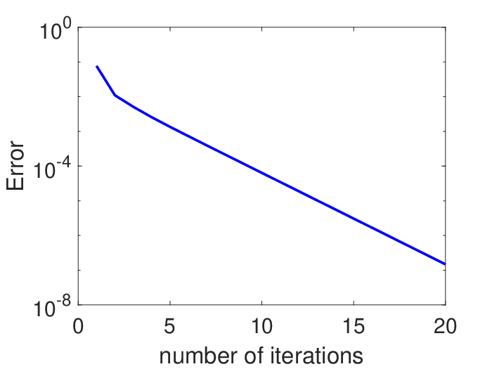
Here, the free parameter is chosen as for the fastest convergence. The iterative process is controlled by the error between two consecutive iterations given by
and the stabilization factor error given by The residue of the interaction process is determined by where

The periodic standing wave solution of the fNLS equation with is given in [5] as
| (6.9) |
where . Here the fundamental period is where is the complete elliptic integral of first kind.


In order to test the accuracy of our scheme, we compare the exact solution (6.9) with the numerical solution obtained by using (4.20) as the initial guess. The space interval is and number of grid points is chosen as . In the first panel of Figure 6.1, we present the exact and numerical solutions for the frequency . As it is seen from the figure, the exact and the numerical solutions coincide. In the other panels of Figure 6.1, the variations of three different errors with the number of iteration are presented. These results show that our numerical scheme captures the solution remarkably well.
The exact solutions of the fNLS equation are not known for . In Figure 6.2 we illustrate the periodic wave profiles for several values of with . The nonlinear term becomes dominant with decreasing values of . Therefore, the wave steepens as expected. In the rest of the numerical experiments, we investigate the sign of q in for different values of . The interval is discretized into subintervals. For each value of , we generate the periodic wave profile by using the Petviashvili’s iteration method on the interval by choosing . We use the forward difference method for the numerical differentiation with respect to after performing the numerical integration.
In Figure 6.3 we illustrate the variation of q with for , and where the axis is in the logarithmic scale. As it is seen from the figure, q is negative. Numerical results indicate that the periodic wave is orbitally unstable for .


The variation of q with for and is depicted in Figure 6.4. Numerical results show the orbital stability of the periodic wave for as q is positive.
We have performed numerical experiment for several values of . We observe that the value of q is always negative for and it is always positive for . However, for the values the numerical results indicate that there is critical wave frequency such that q is negative for and positive for . In Figure 6.5 the variation of q with for and is presented.


Appendix A Basic facts on positive operators
Here, we present important facts (verbatim) contained in [1, Section 2] and [6]. Let the fixed represent the frequency of the periodic wave which solves equation . For , we define the operator by
for all , where and represents the symbol of the fractional Laplacian given by (1.2). Since , we have
is a Hilbert space with norm endowed by the inner product
where and
By [6, Proposition 3.2], we see that is well-defined and it defines a compact and self-adjoint operator defined in . By the spectral theorem for compact and self-adjoint operators, there exists an orthonormal basis formed by eigenfunctions of the operator and corresponding eigenvalues whose only possible accumulation point is zero. In addition, the eigenvalues can be enumerated of the form
According to [6, Corollary 3.1], we have the following important result: is an eigenvalue of if and only if is an eigenvalue of the operator (as an operator of with domain ). Moreover, both eigenvalues have the same multiplicity.
Next, for the operator is defined by
| (A.1) |
where
| (A.2) |
is a Hilbert space with norm endowed with the inner product
where
Lemma A.1.
Concerning the operator given by (A.1), we have
- (i)
If is an eigenfunction of for some nonzero eingenvalue, then .
- (ii)
is a compact and self-adjoint operator.
Proof.
(i) Consider satisfying . For all , we have
| (A.3) |
The fact implies that . From the definition of , we obtain by and the Parseval identity (see [37, Corollary 2.54]) that , as desired.
(ii) The action of over the space is given by
where determines a positive measure over the interval and is defined as
Using the Parseval identity we obtain , so that and is a Hilbert-Schmidt operator. By using [38, page 264], we see that is a compact operator.
On other hand, as is an even function, we have that is also an even function and, as a consequence, is a bounded self-adjoint operator since
for all . ∎
By using Lemma A.1 and the spectral theorem for compact self-adjoint operators, we guarantee the existence of an orthonormal complete set formed by eigenfunctions of and satisfying
| (A.4) |
The next result gives us a relationship between the eigenvalues of and .
Lemma A.2.
Suppose that . Consider an orthonormal complete set of eigenfunctions of in such that for all . Then, forms an orthonormal complete set in constituted by eigenfunctions of such that
Proof.
The condition implies that the eigenvalues of are non-zero. In addition, by Lemma A.1 we have for all . By Parseval identity we obtain and thus
Then, by [6, Proposition 3.2] we conclude that for all .
We will prove that is an orthonormal complete set. Consider . Using Parseval identity, we have
for some constant . Thus, implies that . Using similar arguments, it is possible to show that implies .
Next, let be fixed. By Parseval indentity and using the arguments above, we can conclude that Considering , we obtain the basic and useful equality given by Now, suppose that satisfies for all . Thus, for all . Since is a orthonormal complete set in , we have that in . On other hand, since and , we have that in , that is, in , and therefore in . ∎
Remark A.3.
It should be noticed that, if then is one-to-one. Indeed, for a given such that , then which implies . This information is very useful since we have that is an orthonormal complete set in .
Acknowledgments
G. de Loreno and G. E. B. Moraes are supported by the regular doctorate scholarship from CAPES/Brazil. F. Natali is partially supported by Fundação Araucária/Brazil (grant 002/2017), CNPq/Brazil (grant 304240/2018-4) and CAPES MathAmSud (grant 88881.520205/2020-01).
References
- [1] Albert, J., Positivity properties and stability of solitary-wave solutions of model equations for long waves, Commun. PDE., 17 (1992), 1-22.
- [2] Amann, H., Compact embeddings of vector-valued Sobolev and Besov spaces, Glas. Mat. Ser. III, 35 (2000), 161-177.
- [3] Amaral, S., Borluk, H., Muslu, G., Natali, F. and Oruc, G., On the existence, uniqueness and stability of periodic waves for the fractional Benjamin-Bona–Mahony equation, Stud Appl Math., (2022), 148:62-98.
- [4] Ambrosio, V., On some convergence results for fractional periodic Sobolev spaces, Opuscula Math., 40 (2020), 5-20.
- [5] Angulo, J., Nonlinear stability of periodic travelling-wave solutions for the Schrödinger and modified Korteweg–de Vries equation, J. Differential Equations, 235 (2007), 1-30.
- [6] Angulo, J. and Natali, F.,Positivity properties of the Fourier transform and the stability of periodic travelling-wave solutions, SIAM J. Math. Anal., 40 (2008), 1123-1151.
- [7] Berger, M. and Schechter, M., Embedding theorems and quasi-linear elliptic boundary value problems for unbounded domains, Trans. Amer. Math. Soc., 172 (1972), 261-278.
- [8] Bisci, G., Radulescu, V. and Servadei, R., Variational methods for nonlocal fractional problems, Cambridge University Press, Cambridge, 2016.
- [9] Blanchard, P. and Brüning, E., Mathematical methods in Physics: Distributions, Hilbert space operators, variational methods, and applications in quantum physics, Birkhäuser/Springer, Cham, 2015.
- [10] Boling, G., Yongqian H. and Xin, J., Existence of the global smooth solution to the period boundary value problem of fractional nonlinear Schrödinger equation, Appl. Math. Comput., 204 (2008), 468-477.
- [11] Bottman, N., Nivala, M. and Deconinck, B., Elliptic solutions of the defocusing NLS equation are stable, J. Phys. A., 44 (2011), 285201.
- [12] Boyd, R., Nonlinear optics. Third edition. Elsevier/Academic Press, Amsterdam, 2008.
- [13] Bruell, G. and Dhara, R. N. Waves of maximal height for a class of nonlocal equations with homogeneous symbol, Indiana Univ. Math. J., 70 (2021), 711-742.
- [14] Buffoni, B., and Toland, J. Analytic theory of global bifurcation. Princeton University Press, Princeton, 2016.
- [15] Cazenave, T., Semilinear Schrödinger equations. American Mathematical Society, Providence, 2003.
- [16] Cazenave T. and Lions. P.-L., Orbital stability of standing waves for some nonlinear Schrödinger equations, Comm. Math. Phys., 85 (1982), 549-561.
- [17] Chen, A., Wen, S. and Huang, W. Existence and orbital stability of periodic wave solutions for the nonlinear Schrödinger equation, J. Appl. Anal. Comput., 2 (2012), 137-148.
- [18] Cho, Y., Hwang, G., Kwon, S. and Lee, L., Well-posedness and ill-posedness for the cubic fractional Schrödinger equations, Discrete Contin. Dyn. Syst., 35 (2015), 2863-2880.
- [19] Claassen, K. and Johnson, M., Nondegeneracy and stability of antiperiodic bound states for fractional nonlinear Schrödinger equations, J. Differential Equations, 266 (2019), 5664-5712.
- [20] Cristófani F., Natali F. and Pastor A., Periodic traveling-wave solutions for regularized dispersive equations: sufficient conditions for orbital stability with applications, Commun. Math. Sci., 18 (2020), 613-634.
- [21] Deconinck, B. and Upsal, J., The orbital stability of elliptic solutions of the focusing nonlinear Schrödinger equation, SIAM J. Math. Anal., 52 (2020), 1-41.
- [22] Demirbas, S., Erdoğan, M. and Tzirakis, N., Existence and uniqueness theory for the fractional Schrödinger equation on the torus, some topics in harmonic analysis and applications, Adv. Lect. in Math., 34 (2016), 145-162.
- [23] Duran, A., An efficient method to compute solitary wave solutions of fractional Korteweg–de Vries equations, Int. J. Comput. Math. 95 (2018), 1362–1374.
- [24] Duran, A. and Álvarez, J., Numerical generation of periodic traveling wave solutions of some nonlinear dispersive wave systems, J. Comput. Appl. Math., 316 (2017), 29-39.
- [25] Fibich, G., The nonlinear Schrödinger equation. Singular solutions and optical collapse. Springer, Cham, 2015.
- [26] Frank, R. and Lenzmann, E., Uniqueness of non-linear ground states for fractional Laplacians in . Acta Math. 210 (2013), 261-318.
- [27] Gallay, T. and Hărăguş, M., Stability of small periodic waves for the nonlinear Schrödinger equation, J. Differential Equations, 234 (2007), 544-581.
- [28] Gallay, T. and Hărăguş, M., Orbital stability of periodic waves for the nonlinear Schrödinger equation, J. Dynam. Differential Equations, 19 (2007), 825-865.
- [29] Gallay, T. and Pelinovsky, D., Orbital stability in the cubic defocusing NLS equation: I. Cnoidal periodic waves, J. Differential Equations, 258 (2015), 3607-3638.
- [30] Grillakis, M., Shatah, J. and Strauss, W., Stability theory of solitary waves in the presence of symmetry I, J. Funct. Anal., 74 (1987), 160-197.
- [31] Grillakis, M., Shatah, J. and Strauss, W., Stability theory of solitary waves in the presence of symmetry II, J. Funct. Anal., 94 (1990), 308-348.
- [32] Gustafson S., Le Coz S. and Tsai T-P., Stability of periodic waves of 1D cubic nonlinear Schrödinger equations, Appl. Math. Res. Express., (2017), 431-487.
- [33] Hakkaev, S. and Stefanov, A., Stability of periodic waves for the fractional KdV and NLS equations, Proc. Roy. Soc. Edinburgh Sect. A., 151 (2021), 1171-1203.
- [34] Hur, V. and Johnson, M., Stability of periodic traveling waves for nonlinear dispersive equations, SIAM J. Math. Anal., 47 (2015), 3528-3554.
- [35] Hur, V., Johnson, M. and Martin, J., Oscillation estimates of eigenfunctions via the combinatorics of noncrossing partitions, Discrete Anal., (2017), 13, 20 pp.
- [36] Ionescu, A. and Pusateri, F., Nonlinear fractional Schrödinger equations in one dimension, J. Funct. Anal., 266 (2014), 139-176.
- [37] Iorio, R. J. Jr. and Iorio, V. M. V., Fourier Analysis and Partial Differential Equations, Cambridge University Press, Cambridge, 2001.
- [38] Kato, T., Perturbation theory for linear operators. Reprint of the 1980 edition. Springer-Verlag, Berlin, 1995.
- [39] Kirkpatrick, K., Lenzmann, E. and Staffilani, G. On the continuum limit for discrete NLS with long-range lattice interactions, Comm. Math. Phys., 317 (2013), 563-591.
- [40] Klein, C., Sparber, C. and Markowich, P. Numerical study of fractional nonlinear Schrödinger equations, Proc. Math. Phys. Eng., 470.2172 (2014): 20140364.
- [41] Laskin, N., Fractional quantum mechanics and Lévy path integrals, Phys. Lett. A, 268 (2000), 298-305.
- [42] Laskin, N., Fractional Schrödinger equation, Phys. Rev. E, 66 (2002), 056108.
- [43] Le, U. and Pelinovsky, D., Convergence of Petviashvili’s method near periodic waves in the fractional Korteweg-de Vries equation, SIAM J. Math. Anal., 51 (2019), 2850-2883.
- [44] Leisman, K., Bronski, J., Johnson, M. and Marangell, R., Stability of traveling wave solutions of nonlinear dispersive equations of NLS type, Arch. Ration. Mech. Anal., 240 (2021), 927-969.
- [45] Ma, Y. and Ablowitz, M., The periodic cubic Schrödinger equation, Stud. Appl. Math., 65 (1981), 113-158.
- [46] Natali F., Le U. and Pelinovsky D., New variational characterization of periodic waves in the fractional Korteweg-de Vries equation, Nonlinearity, 33 (2020), 1956-1986.
- [47] Natali F., Le U. and Pelinovsky D., Periodic waves in the fractional modified Korteweg-de Vries equation, J. Dynam. Diff. Eqts., (2021), 1-40.
- [48] Natali, F., Moraes, G., de Loreno, G. and Pastor, A. Cnoidal Waves for the Klein-Gordon and Nonlinear Schrödinger Equation, Preprint, (2021).
- [49] Natali, F. and Pastor, A., The Fourth-Order Dispersive Nonlinear Schrödinger Equation: Orbital Stability of a Standing Wave, SIAM J. Appl. Dyn. Syst., 14 (2015), 1326-1347.
- [50] Nirenberg, L., On elliptic partial differential equations, Ann. Scuola. Norm. Sup. Pisa. Cl. Sci., 13 (1959), 115-162.
- [51] Oruc, G., Borluk H. and Muslu, G., The generalized fractional Benjamin-Bona-Mahony equation: Analytical and numerical results, Phys. D, 409 (2020), 132499.
- [52] Pelinovsky, D. and Stepanyants, Y., Convergence of Petviashvili’s iteration method for numerical approximation of stationary solution of nonlinear wave equations, SIAM J. Numer. Anal., 42 (2004), 1110-1127.
- [53] Rabinowitz, P., On a class of nonlinear Schrödinger equations, Z. Angew. Math. Phys., 43 (1992), 270-291.
- [54] Reed, M. and Simon, B., Methods of modern mathematical physics. IV. Analysis of operators. Academic Press, New York-London, 1978.
- [55] Roncal, L. and Stinga, P., Fractional Laplacian on the torus, Commun. Contemp. Math., 18 (2016), 1550033.
- [56] Rowlands, G., On the stability of solutions of the Non-linear Schrödinger equation, J. Appl. Math., 13 (1974), 367-377.
- [57] Sulem, C. and Sulem, P.-L., The nonlinear Schrödinger equation. Self-focusing and wave collapse. Springer-Verlag, New York, 1999.
- [58] Thirouin, J., On the growth of Sobolev norms of solutions of the fractional defocusing NLS equation on the circle, Ann. Inst. H. Poincaré Anal. Non Linéaire, 34 (2017), 509-531.
- [59] Triebel, H., Interpolation theory, function spaces, differential operators. Johann Ambrosius Barth, Heidelberg, 1995.
- [60] Triebel, H., Theory of Function Spaces. Reprint of the 1983 edition. Birkhäuser/Springer Basel AG, Basel, 2010.
- [61] Weinstein, M., Modulational stability of ground states of nonlinear Schrödinger equations, SIAM J. Math. Anal., 16 (1985), 472-491.