Power Allocation Algorithms for
Massive MIMO Systems with Multi-Antenna Users
Abstract
Modern 5G wireless cellular networks use massive multiple-input multiple-output (MIMO) technology. This concept entails using an antenna array at a base station to concurrently service many mobile devices that have several antennas on their side. In this field, a significant role is played by the precoding (beamforming) problem. During downlink, an important part of precoding is the power allocation problem that distributes power between transmitted symbols. In this paper, we consider the power allocation problem for a class of precodings that asymptotically work as regularized zero-forcing. Under some realistic assumptions, we simplify the spectral efficiency functional and obtain tractable expressions for it. We prove that equal power allocation provides optimum for the simplified functional with total power constraint (TPC). We propose low-complexity Intersection Methods (IM) that improve equal power allocation in the case of per-antenna power constraints (PAPC). On simulations using Quadriga, the proposed IM method in combination with widely-studied Water Filling (WF) shows a significant gain in spectral efficiency while using a similar computing time as the reference Equal Power (EP) solution.
keywords
5G, MIMO, Multi-antenna UE, Precoding, Regularized Zero-Forcing, Power Allocation, MMSE-IRC Detection, Constrained Optimization, Karush–Kuhn–Tucker conditions, Asymptoticsb Huawei Technologies, Russian Research Institute, Moscow Research Center
c A. Ishlinsky Institute for Problems in Mechanics RAS
1 Introduction
The massive multiple-input multiple-output (MIMO) systems have attracted a lot of attention in both academia and industry since their first appearance [1, 2]. The main characteristic of the massive MIMO system is the large-scale antenna arrays at the cellular base station (BS). Using a large number of antennas, the massive MIMO system can exceed the achievable rate of a conventional MIMO [3] system and simultaneously serves (with low power consumption) several users.
A critical issue for improving the performance of wireless networks is the efficient management of available radio resources [4]. Numerous works are dedicated to optimal allocation of the radio resources, for example, power and bandwidth to improve the performance of wireless networks [5].
An important part of signal processing in downlink is precoding since with this procedure we can focus transmission signal energy on smaller regions, which allows achieving greater spectral efficiency with lower transmitted power [6]. Various linear precodings allow directing the maximum amount of energy to the user like Maximum Ratio Transmission (MRT) or completely get rid of inter-user interference like Zero-Forcing (ZF) [7, 8]. The precoding problem is well-studied (see e.g., overview [9, 10, 11] and textbooks [12, 13] and bibliography within), nonetheless there are open questions. For example, most of the works consider the total power constraint (TPC) (see e.g., [14]), the more realistic per-antenna power constraints (PAPC) are much less studied (see e.g., [15, 16]).
An important component of the precoding procedure is the power allocation (PA) problem that is widely discussed in the literature. In [17], by using either the signal-to-interference-and-noise ratio (SINR) or the outage probability as the performance criteria, different power allocation (PA) strategies are developed to exploit the knowledge of channel means. In [18] bounds on the channel capacity are derived for a similar model with Rayleigh fading and channel state information (CSI). The power allocation problem in a three-node Gaussian orthogonal relay system is investigated in [19] to maximize a lower bound on the capacity. Two power allocation schemes based on minimization of the outage probability are presented in [20] for the case when the information of the wireless channel responses or statistics is available at the transmitter. In [21] studies optimal power allocation schemes in a multi-relay cooperating network employing amplify-and-forward protocol with multiple source-destination pairs. The work [22] advocates the use of deep learning to perform max-min and max-prod power allocation in the downlink of Massive MIMO networks. In [23] the total downlink power consumption at the access points is minimized, considering both to transmit powers and hardware dissipation.
The most relevant works to the current paper are of E. Björnson et al. In [12, sec. 7.1] the case of single-antenna user equipment (UE) is studied in detail, targeting UE spectral efficiency and using multi-criteria optimization approach and Pareto front analysis. In [16, p. 328] multi-antenna UEs are considered, but they are supposed to get only one data channel (or stream). The difficulty of the multi-antenna UE case is that the channels between different antennas of one UE are often spatial correlated [24]. Therefore, the matrix of the user channel is ill-conditioned (or even has incomplete rank) thus one can not efficiently transmit data using the maximum number of streams. To solve this problem, instead of the full matrix of the user channel, vectors from its singular value decomposition (SVD) with the largest singular values are used for precoding [25]. When the number of streams (UE rank) is greater than one, it is necessary to consider the phenomenon of effective Signal-to-Interference-and-Noise-Ratio (effective SINR) [26]. In [27] a dynamic optimization model which maximizes the total energy efficiency along with satisfying the necessary QoS constraints is proposed. In [28] a novel approach to joint optimal power allocation and user association techniques in which cells are powered via a common grid network and alternative energy resources is suggested. In [29] a dynamic optimization model to minimize the overall energy consumption of 5G heterogeneous networks is proposed.
In this paper, we study the problem of power allocation (PA) of MIMO wireless systems with users with multiple antennas and generalize the results of E. Björnson et al. for the case of multi-antenna UEs with rank greater than one. We present the novel solutions to the PA problem that maximize network throughput in terms of spectral efficiency (SE) subject to either total or per-antenna power constraints. The original problem is not convex, but we managed to simplify it to a convex one with additional assumptions on the system model, e.g., applying a specific class of detection. Under some natural assumptions, we simplify the spectral efficiency functional and prove that the uniform power allocation provides its optimum subject to TPC. For the case of PAPC, we equivalently reformulate the optimization problem as the Lagrange system of equations and write down the Karush–Kuhn–Tucker conditions. Here, algorithmic solutions of PA problem are proposed assuming realistic PAPC.
The simulation results based on Quadriga channel simulator [30] show the effectiveness of the proposed algorithmic approach in comparison with the reference PA schemes. To the authors’ best knowledge, these mathematical results are new.
The rest of this paper is organized as follows. After this Introduction, Section 2 is devoted to the channel and system model where we introduce the downlink MIMO channel model, reference precoding methods, various detection schemes, and quality measures. In Section 3 we show a simplification of the PA problem, where we describe asymptotic diagonalization property of precoding matrices are used, proof of similarity of Conjugate and MMSE-IRC matrices, and Effective SINR models. In Section 4 we consider the problem of the PA algorithm under TPC and PAPC assumptions, where we describe equal power allocation under the TPC, and the solution under the PAPC assumptions. We also consider problem-solving taking into account Modulation and Coding Scheme (MCS) (4.2). The numerical algorithm description is presented in Section (4.5). Numerical experiments to compare considered algorithms are provided in Section 5. Algebraic notations and reference values are shown in Tab. 1.
| Symbols | Notations |
|---|---|
| Channel, precoding and detection matrices | |
| -th column of matrix | |
| -th row of matrices | |
| -th element of matrices | |
| Diagonal matrix of singular values | |
| the number of users | |
| the number of transmit antennas | |
| the total number of receive antennas | |
| the number of receive antennas for each user | |
| the total number of layers in the system | |
| the number of layers for each user | |
| Complex conjugate operator |
2 Channel and System Model
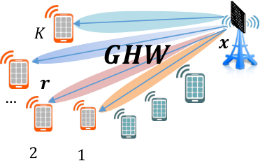
According to [13, 12, 31, 32] we consider a MIMO broadcast channel. Symbol is a received vector, and is a sent vector, and is a channel matrix, and is a Precoding matrix, and is a block-diagonal detection matrix, is a noise-vector, is a vector of sending symbols. Note that the linear precoding and detection are implemented by simple matrix multiplications. The constant is the number of transmit antennas, is the total number of receive antennas, and is the total number of transmitted symbols in the system. Usually, they are related as . Each of the matrices decomposes by users, so please see the scheme in Fig. 2. The Multi-User MIMO model is described using the following linear system:
| (1) |
In this paper, we make the following assumptions: i) that all users’ channels are subject to uncorrelated Rayleigh fading, and ii) that the transmitter has perfect CSI of all downlink channels. This assumption is reasonable in time division duplex (TDD) systems because it enables the transmitter to use reciprocity to estimate the downlink channels. iii) that each user only has access to their own CSI.
2.1 Singular Value Decomposition of the Channel
The channel matrix for user , contains channel vectors by rows. The path loss diagonal matrix contains singular values in decreasing order along its main diagonal. It is convenient [25] to represent via its Singular Value Decomposition (SVD): .
Lemma 1 (Main Decomposition).
Lemma 1 means that by collecting all users together, we can write a specific channel matrix decomposition [33]. Note, that such decomposition is not a convenient SVD of the channel matrix , and the matrix is not unitary. But it consists of the SVDs of the size and has block-diagonal unitary left matrix . We use this form in the construction of the optimal detection matrix [25].
Usually, the transmitter sends to UE several layers and the number of layers (rank) is less than the number of UE antennas (). In this case, it is natural to choose for transmission the first vectors from that correspond to the largest singular values from . Denote by the first largest singular values from , and by the first left and right singular vectors that correspond to :
| (2) |
i.e. . Numbers (and particular selection of ) are defined during the Rank Adaptation problem that, along with Scheduler, is solved before precoding. For the Rank adaptation problem, we refer for example to [34] and in what follows we consider , already chosen.
2.2 Precoding Matrices
The precoding matrix is responsible for the beamforming from the base station to the users [35]. The linear methods for precoding do the following. Firstly, the linear solutions obtain singular value decomposition for each user (Lemma 1) and take the first singular vectors which attend to the first greatest singular values [25]. All these matrices are concatenated to the one matrix , which is used as the main building block of these precoding constructions. Finally, the precoding matrix is constructed from the obtained singular vectors. We describe linear methods for constructing a precoding matrix.
We are considering precoding matrices in the following form:
| (3) |
where is taken from the specific SVD decomposition from Lemma 1 and is a diagonal matrix of power allocation.
Let us repeat some known precodings that are considered as initial solutions for studied power allocation methods.
The inter-user interference is vanished by the Zero-Forcing (ZF) precoding [7]:
| (4) |
It can be improved by using Regularized Zero-Forcing (RZF) precoding:
| (5) |
where the regularization parameter depends on noise level and average path-losses [36].
Further improvement is possible with diagonal regularization as in Adaptive Regularized Zero-Forcing (ARZF) [33] precoding (this idea was discussed in [12, 37], the following explicit heuristic formula for the MU MIMO case was proposed and studied in [33]):
| (6) |
Detailed comparison of these algorithms and bibliography can be found in [33].
2.3 Detection Matrices
After precoding and transmission, on the side of UE , we have to choose a detection matrix , which takes into account the rank of UE . The way the UE performs detection strongly affects overall performance, and different detection algorithms require different optimal precoding matrices (see [36], where precoding is chosen as a function of the detection matrix). The best way would be to consistently choose precoding and detection, but this is hardly possible due to the distributed nature of wireless communication. However, there are ideas on how to set up a precoding matrix, assuming a specific detection method on the UE side in the transmitter [38]. We do not consider such an approach in our work, although it can be used to further improve our main proposal.
We assume the effective channel matrix to be calculated on the UE side. The Minimum Mean Square Error (MMSE) detection for the user , where is the regularization value [39, 40], performs as follows:
| (7) |
In this paper, priority is given to the MMSE-Interference-Rejection-Combiner (MMSE-IRC) detection [41]:
| (8) |
And covariance matrix of total intra-user interference:
| (9) |
To conduct analytical calculations, we assume virtual Conjugate Detection (CD) in the following form [33]:
| (10) |
where is a corresponding to -th user sub-matrix of matrix in equation (3).
2.4 Quality Measures
We measure the quality of precoding using well-known functions such as Signal-to-Interference-and-Noise-Ratio (SINR) [42] and Spectral Efficiency (SE) [43]. These functions are based not on the actual sending symbols , but some distribution of them [44]. Thus, we get the common function for all assumed symbols, which can be sent using the specified precoding matrix. We denote as the set of symbols for -th user. The SINR function is defined as:
| (11) |
For simulations of a physical layer (PHY) in multi-carrier and multi-layer OFDM systems an effective SINR mapping (ESM) model is used. Such model compresses the given set of SINRs experienced by the receiver over every sub-channel into a single scalar value (called effective SINR). According to the paper [26], the effective SINR for a user is calculated using the SINR at each layer of each Resource Block (RB) as follows. Functions and are table-defined (see, e.g., Table 5 for ). Assuming only one RB, we can define as a self-consistent solution of the following system:
| (12) |
2.5 Problem Statement
We consider the channel model in the form (1) that particularly means exact measurements of the channel. To further simplify the problem we suppose detection policy to be a known function, moreover we assume Conjugate Detection (10) that simplifies the channel model to (24). Based on this channel model, we calculate SINR of transmitted symbols by (11) and effective SINR of UE, which can be approximately calculated by (12) and (29). We denote the total power of the system as, , assuming in the experiments.
The total power constraint and the more realistic per-antenna power constraints (see [12]) impose the following conditions on the precoding matrix. Since case is considered in this paper, conditions read:
| (14) |
3 Simplifications of the Problem
3.1 Asymptotic Diagonalization Property of Precoding
Definition 2.
Let us assume the case of small noise and denote and is some diagonal matrix. In real systems, Scheduler algorithms choose UE for pairing if this assumption is fulfilled. Define the property of asymptotic diagonalization of as of precoding matrix as follows:
| (16) |
Precoding algorithms: ZF (4), RZF (5), and ARZF (6) satisfy the property (16). This can be easily shown with the Neumann series as in the following Lemma (it is similar to [33, Lemma 2]).
Lemma 3.
Consider square invertible complex matrices and of the same size and rank. For any and the following matrix identity is true: .
Proof.
| (17) |
| (18) |
| (19) |
∎
3.2 The Similarity of Conjugate Detection and MMSE-IRC
In this section, we prove the similarity of MMSE-IRC (8) [41] and Conjugate Detection (CD) (10) [33]. Detection CD does not depend on precoding and allows to significantly simplify the considered problem (15). First, we prove some useful properties about CD (compare with [33, Theorem 1]).
Lemma 4.
Proof.
Necessity. Using Lemma (1) we can write
| (25) |
which immediately leads to (24).
Sufficiency. Assume that (23) holds, then , since the matrix . Then, expansion of vector in basis is unique. The elements of the matrix are the coefficients of this expansion. Therefore, a matrix with the property (23) is unique.
The last equivalence in (23) is true due to the block diagonality of the matrix . ∎
Theorem 5.
Proof.
We need the following consequence of the (16) property:
| (26) |
Taking into account the form of we can rewrite [48]:
∎
Remark 2.
The introduced CD detection is speculative: it hardly can be implemented in practice. UE measures via pilot signals instead of . Nonetheless, it is very useful for theoretical research. Moreover, the asymptotic behavior of MMSE and MMSE-IRC detection is similar to that of CD (Sec. 3.2). Particularly, if precoding is Zero-Forcing (4) and the noise power is zero (), then ; if, additionally, precoding has the full rank, then .
Remark 3.
Lemma 4 shows that the assumption that UEs use CD on their side sufficiently simplifies the initial problem, decreases its dimensions, and allows notation to be uniform. Namely, we can work with user layers of shapes and instead of considering user antennas space. Note also that for precoding it is sufficient to only perform Partial SVD of the channel , keeping just the first singular values and vectors for each user : .
Based on this, in what follows we can omit the tilde and write instead of correspondingly.
3.3 Low Correlated Users
We define an interference-correlation matrix as . In real networks, the set of UEs is chosen by Scheduler and the number of layers of each UE is chosen to be fixed by the Rank Selection algorithm. Both Scheduler and Rank Selection methods provide , where is the noise-power ratio. Thus, we assume user correlation to be low compared to noise power, which means .
Lemma 6.
For precoding satisfying the property (16) and inference-correlation matrix satisfying , is the noise-power ratio, it is asymptotically true that .
Proof.
| (27) |
∎
Using Lemma 6 we immediately get the following
Theorem 7.
| (28) |
Proof.
∎
3.4 Effective SINR Models
In this subsection, we compare two models of Effective SINR from [45, 26, 33]. In theoretical calculations, model (12) is extremely inconvenient. To simplify the formula of effective SINR (12), we average per-symbol SINRs (11) by the geometric mean, where denotes the set of symbols for -th user:
| (29) |
Fig. 4 shows the dependencies of for a user with four antennas to justify the close relationship of the various SINR averaging (12) and (29). The axis is the average SINR in dB: .
Fig. 4 shows the comparison of effective SINR in the form of the geometric mean and the form of different MCS- values. Differences between various effective SINRs can take values greater than five decibels. On the other hand, points SINR with a large difference in the maximum and minimum values are unusual in practice.

For precoding satisfying the property (16) and from the formula for SINR (28) with a CD using the geometric mean effective SINR model (29), we can write the SINR for the -th user as follows:
| (30) |
The formula (30) reflects the channel quality for the specified user without considering other users. The value of depends on the singular values (related to matrices ), the transmitted power and noise . This function will be used in theoretical calculations due to its simplicity.
3.5 Spectral Efficiency Simplification
In this section we simplify optimization problem of Spectral Efficiency maximization in case of Zero-Forcing algorithms with asymptotic diagonalization property (16), Conjugate detection matrix (10), geometrical averaging of effective SINR model (30) and low correlated users (see Lemma 6).
For any it is true that: , and so
| (31) |
We simplify the initial optimization problem by maximization of its leading term:
| (32) |
These problems are not equivalent, although their solutions are close to each other. If we calculate by ZF algorithm, that gives zero interference, then SINR is as follows
| (33) |
and maximization of the leading term gives
Finally, we can reduce tasks (15) (a) and (b) to the following problems:
| (34) |
4 Solutions of the Problem
According to [12, sec. 7] we consider equal transmit power strategy for all users. Such power allocation gives the maximum for a reasonable lower bound on the (13) under some feasible assumptions. Although this Power allocation is not optimal, these heuristics provide a good suboptimal solution.
4.1 Simplified PA Problem with Total Power Constraints
Theorem 8.
Proof.
4.2 EESM Model and Total Power Constraints
By analogy with the formulas (31 and 32) we can calculate Spectral efficiency using physical MCS- model (12), where the parameter for each depends on given and therefore depends on the precoding matrix, in particular on power allocation variables for all :
| (38) |
The function (38) is discontinuous. Nevertheless, if we fix for all , this function becomes smooth from . For example, we can take from point as . Next, write SINR similar to Eq. (28) without interference as ( does not depend on ). We can write Lagrangian for the problem 15 (a):
| (39) |
And its partial derivatives concerning .
| (40) |
where and .
We can write Karush–Kuhn–Tucker conditions:
| (41) |
And its solution is (see proof in Appendix 6.2):
| (42) |
where:
| (43) |
4.3 Simplified PA Problem with Per-Antenna Power Constraints
Theorem 9.
Proof.
The problem (15) (b) can be reduced to a task
| (45) |
To solve it, we can use the Karush-–Kuhn-–Tucker conditions. Lagrangian has the form
| (46) |
If and are the optimum of the optimization problem, then they satisfy the following conditions
| (47) |
We take .
For geometric reasons, the original optimization problem has a solution; therefore, there is at least one solution to the system (47).
The resulting system can be solved by brute force on the set of zeroed lambdas. Let’s say we have non-zero lambdas. Consider the cases.
- 1.
, in this case the linear system will be inconsistent since the number of equations is greater than the number of unknowns () and the system itself (47) will not have a solution.
- 2.
, in this case the linear system has exactly one solution, and the system itself (47) has at most one solution.
- 3.
. This case reduces to the system of quadratic equations. If is a matrix consisting of rows of matrix corresponding to nonzero lambdas, then
(48) Here and is the orthogonal complement to .
- 4.
, in this case, there are one nonzero lambda. Let therefore
(49)
∎
4.4 EESM Model and Per-Antenna Power Constraints
In this section, we combine two ideas of previous sections. We calculate Spectral efficiency (38) using exponential model (12) for the fixed value. Using this, we can write Lagrangian for the problem 15 (b) and its partial derivatives concerning :
| (50) |
| (51) |
The Karush-–Kuhn-–Tucker conditions:
| (52) |
The resulting system can be solved by brute force on the set of zeroed lambdas. Let’s say we have non-zero lambdas. Consider the cases.
- 1.
, in this case the linear system will be inconsistent since the number of equations is greater than the number of unknowns () and the system itself (52) will not have a solution.
- 2.
, in this case the linear system has exactly one solution, and the system itself (52) has at most one solution.
- 3.
. If is the set of indexes of nonzero lambda, then this case reduces to the system of following equations:
(53) - 4.
, in this case there are one nonzero lambda. Let therefore
| (54) |
where:
| (55) |
The proof is similar to the proof of Eq. (42) which can be found in the Appendix.
4.5 Heuristic Algorithms, based on KKT-analysis
In this section we proposed two algorithms for SE maximization in the case of PAPC of two different models of Effective SINR. The first Alg. 1 assume Geometrical Averaging model (29), while the second Alg. 2 uses the proper EESM model (12)
Define smooth target function . For example, using (11), (13) and (12);
Calculate the hyperplane on which the square of the starting point lies. The index of this hyperplane is the maximal row norm: ;
Both Alg. 1 and Alg. 2 take equalizing powers as the first approximation of the vector (see Point on Fig. 5). Then it finds the hyperplane on which the given point lies and searches on this hyperplane for the optimal (Point ). To find the optimal point, we use the Eq. (49) for the Alg. 1 and by Eq. (54) for Alg. 2.
If the obtained point is satisfied with the Power Constrains, then this is the result of the algorithm. This point may not be satisfied with the Power Constraints. In this case, we construct a beam from the starting point to the optimal point. The first intersection with other hyperplanes (Point ) is a result of the algorithms. The formula for Point can be negative or zero. In this rare case, the result of the algorithm is Point .
Fig. 6 shows the transmitted symbol powers using Alg. 1 (IM) compared to the EP method. The SINR values in dB of each layer are also given for comparison. It is shown that the SINR values increase for those symbols for which the power increases. And vice versa, the SINR decreases for those symbols for which the power decreases. The total precoding power increases with the use of Alg. 1 (IM).
4.6 Computational Complexity
In terms of complexity, the IM algorithms have the same order as the EP algorithm.
| Variable | Summations | Multiplications | Special operations |
| and | |||
| comparisons | |||
| and (Alg 1) | |||
| and (Alg 2) | calculations of logarithm | ||
| comparisons | |||
| Algorithm | Summations | Multiplications | Special operations |
| EP | |||
| IM (Alg 1) | comparisons | ||
| IM CD, IM IRC(Alg 2) | comparisons, logs | ||
| WF | comparisons, 1 sort |
In Tab. 2 computational complexity of each intermediate step of the algorithms 1, 2 and computational complexity of EP, IM, IM CD, IM IRC and WF algorithms are presented. For these algorithms we assume that we already calculate matrix . For algorithms IM CD, IM IRC and WF we need precalculate matrices , and respectively. The difficulty of calculating some parts can be reduced. For example, when you calculating , you may not consider intersections with some hyperplanes. Note that for calculation of Alg. 2 we need to calculate matrix .
The final complexity of the aforementioned algorithms is .
5 Simulation Results
5.1 Channel Dataset
The datasets generated and analysed during the current study are available in the GitHub repository, https://github.com/eugenbobrov/Power-Allocation-Algorithms-for-Massive-MIMO-Systems-with-Multi-Antenna-Users
To generate channel coefficients, we use Quadriga [30], open-source software for generating realistic radio channel impulse responses. We consider the Urban Non-Line-of-Sight [49] scenarios. For each seed, we generate the random sets of user positions and compute channel matrices for the obtained configurations of users. Example of the random generation of users for Urban setup: there are two buildings, and the users are assigned to either a cluster in a building or to the ground near the building. The parameters of the experiments are listed in Table 1. We describe the generation process in detail in our work [33].
5.2 Numerical Experiments
We compare different PA algorithms based on RZF precoding. Primarily, the comparison involves precoding with the base power (BP) method — native method without PA, and the power equalization algorithm (37). Also, we consider some algorithms based on Karush-Kuhn-Tucker conditions (47). In Tab. 3 algorithms with different parameters of the target optimization function, the power constraints and the starting point for intersection methods used for RZF method are presented.
For reference we use the Power Allocation methods from the works of E. Bjornson et al., namely Equal Power (EP) and Water-Filling (WF) that are derived in assumption of Total Power Constraints (TPC). Proposed Intersection Methods (IM) are constructed to maximize Spectral Efficiency (SE) taking into account Per-Antenna Power Constraints (PAPC) and gives gains over the EP and WF methods in the specified region. Additionally, the IMs method can use WF solution as the starting point to achieve the cumulative gain in SE. This result is shown in Fig. 9.
| Algorithm | Optimization Function | Constraints | Initialization |
|---|---|---|---|
| EP | TPC | - | |
| IM | PAPC | EP | |
| WF | TPC | - | |
| IM CD | PAPC | EP | |
| IM IRC | PAPC | EP | |
| WF IM | PAPC | WF |
In Figs. 7 and 8 we present an average SE (13) from numerical simulations of the proposed Intersection Method (1) IM and algorithm IM IRC with its modifications to MCS- model (2) IM CD and IM IRC and reference BP and EP methods. And in Figs. 9-11 we present their gains over the reference EP method. Percentage gain means expressing the increase in SE value of the considered algorithm as a percentage compared to the baseline, in other words:
| (56) |
All Figs. 7-11 claim SE improvement of the proposed algorithms over the baseline EP method. Fig. 9 shows SE gain assuming Geometric Mean Effective SINR (29), while Figs 10 and 11 assume the Exponential Averaging model (12). Both the IM and IM IRC algorithms provide better power allocation (PA) under per-antenna power constraint (PAPC), which means better value of Spectral Efficiency (13) of the obtained precoding in comparison to the BP and EP methods.
In Fig. 12 we present the distribution of power allocated to different layers () in case of PAPC when SU SINR is equal to 15dB. Cumulative distribution function (CDF) is calculated over transmitted layers. Here we see that IM majorizes both BP and EP methods in terms of power of layers (while still preserving PAPC), which is the main source of IM gains. In contrast, the WF method makes redistribution of power from UE with lower SINR to UE with higher SINR, which can be unfair and lead to blocking of cell-edge UE due to their poor contribution to the SE function. The WF IM (IM method applied to WF initial distribution) also majorizes WF and partially fixes its unfairness.
Presented experiments claim that the proposed method IM outperforms the reference EP up to 5% at the low SUSINR region ( dB) and up to 2% at high ( dB). The modification of the algorithm IM IRC provides better results up to 6% at the low SUSINR region. This is the result of better distribution of transmitted symbol powers (see example on Fig. 6).
The proposed IM method in combination with widely-studied Water Filling (WF) [50] show a significant gain in spectral efficiency while using a similar computing time as the reference Equal Power (EP) solution (see Fig. 9.)
The assumption that the noise-power ratio is close to zero was chosen that the Equal Power (EP) and Water-Filling (WF) method are close enough. Now we provide experiments both for EP and WF methods in Fig. 9 in a wide range of noise-power ratio. Although theoretical results stay correct only for close to zero noise-power, it helps to derive the Intersection Method (IM), which shows a good performance in a wide range of noise-power ratio.
Finally, it is experimentally proved out that the modification IM CD in case of both table 1 and table 2 MCS- values (see Tab. 5) provides better results than IM. The difference in quality is clear in Gains of SE Figs. 10, 11, which show that the performance improvement of Alg. 2 is because of Alg. 2 utilizes EESM Model 12.
6 Conclusions and Suggested Future Work
In this work, we study the power allocation (PA) problem of wireless MIMO systems with multi-antenna users. We simplify the initial problem using asymptotics of MMSE-IRC detection and SE function when noise and correlations are small. In the case of total power constraint (TPC) the simplified problem can be solved exactly and its solution is Equal Power (EP) distribution. In the case of per-antenna power constraints (PAPC) simplified problem can be further equivalently reformulated as a Lagrange problem for which the Karush–Kuhn–Tucker conditions hold.
Based on such analysis we propose low-complexity heuristic algorithms that provide sub-optimal solutions to the initial PA problem. We study proposed Intersection Methods (IM) on simulations using Quadriga and compare them with Equal Power and Water Filling reference algorithms. When simulated using Quadriga, the proposed IM methods combined with the widely studied Water Filling (WF) show a significant gain in SE using similar computational time compared to the EP baseline solution and allow improving the quality of MIMO systems in the future. Analyzing the CDF of power of layers we show that proposed IM methods majorize considered reference algorithms, provide more power under realistic Per-Antenna Power Constraints (PAPC) constraints and by this way improve Spectral Efficiency.
Since the main focus of this paper is the analytical study of the PA methods, we assume that the base station has perfect channel measurements and neglect all other potential hardware impairments. Nevertheless, the robustness of the noise to a given measurement keeps the current results asymptotically correct and can be carefully considered in future work. There are other possible direction of the future work. Firstly, future work can include a detailed study of PA algorithms, taking into account BLER performance with realistic 5G LDPC coding (e.g. using physical communication system level simulators such as Sionna [51]) rather then approximate effective SINR models such as EESM. Secondly, the more complicated system model considering multiple RBs can be of interest. Thirdly, proposed IM algorithm can be perhaps further improved: improvement of SE can be realized with increasing the complexity of the algorithm, or otherwise, the complexity can be decreased with small decreasing of the SE.
References
- [1] Jeffrey G Andrews, Stefano Buzzi, Wan Choi, Stephen V Hanly, Angel Lozano, Anthony CK Soong, and Jianzhong Charlie Zhang. What will 5G be? IEEE Journal on selected areas in communications, 32(6):1065–1082, 2014.
- [2] Thomas L Marzetta. Noncooperative cellular wireless with unlimited numbers of base station antennas. IEEE transactions on wireless communications, 9(11):3590–3600, 2010.
- [3] Xiaohu Ge, Ran Zi, Haichao Wang, Jing Zhang, and Minho Jo. Multi-user massive MIMO communication systems based on irregular antenna arrays. IEEE Transactions on Wireless Communications, 15(8):5287–5301, 2016.
- [4] Long Le and Ekram Hossain. Multihop cellular networks: Potential gains, research challenges, and a resource allocation framework. IEEE Communications Magazine, 45(9):66–73, 2007.
- [5] Khoa T Phan, Tho Le-Ngoc, Sergiy A Vorobyov, and Chintha Tellambura. Power allocation in wireless multi-user relay networks. IEEE Transactions on Wireless Communications, 8(5):2535–2545, 2009.
- [6] Hien Quoc Ngo, Erik G Larsson, and Thomas L Marzetta. Energy and spectral efficiency of very large multiuser MIMO systems. IEEE Transactions on Communications, 61(4):1436–1449, 2013.
- [7] Tebe Parfait, Yujun Kuang, and Kponyo Jerry. Performance analysis and comparison of ZF and MRT based downlink massive MIMO systems. In 2014 sixth international conference on ubiquitous and future networks (ICUFN), pages 383–388. IEEE, 2014.
- [8] Jiankang Zhang, Sheng Chen, Robert G Maunder, Rong Zhang, and Lajos Hanzo. Regularized zero-forcing precoding-aided adaptive coding and modulation for large-scale antenna array-based air-to-air communications. IEEE Journal on Selected Areas in Communications, 36(9):2087–2103, 2018.
- [9] Nusrat Fatema, Guang Hua, Yong Xiang, Dezhong Peng, and Iynkaran Natgunanathan. Massive MIMO linear precoding: A survey. IEEE systems journal, 12(4):3920–3931, 2017.
- [10] Kan Zheng, Long Zhao, Jie Mei, Bin Shao, Wei Xiang, and Lajos Hanzo. Survey of large-scale MIMO systems. IEEE Communications Surveys & Tutorials, 17(3):1738–1760, 2015.
- [11] Sunil Dhakal. High rate signal processing schemes for correlated channels in 5G networks. 2019.
- [12] Emil Björnson, Jakob Hoydis, and Luca Sanguinetti. Massive MIMO networks: Spectral, energy, and hardware efficiency. Foundations and Trends in Signal Processing, 11(3-4):154–655, 2017.
- [13] David Tse and Pramod Viswanath. Fundamentals of wireless communication. Cambridge university press, 2005.
- [14] Federico Boccardi and Howard Huang. Optimum power allocation for the MIMO-BC zero-forcing precoder with per-antenna power constraints. In 2006 40th Annual Conference on Information Sciences and Systems, pages 504–504. IEEE, 2006.
- [15] Wei Yu. Uplink-downlink duality via minimax duality. IEEE Transactions on Information Theory, 52(2):361–374, 2006.
- [16] Emil Björnson and Eduard Jorswieck. Optimal resource allocation in coordinated multi-cell systems. Now Publishers Inc, 2013.
- [17] Xitirnin Deng and Alexander M Haimovich. Power allocation for cooperative relaying in wireless networks. IEEE Communications Letters, 9(11):994–996, 2005.
- [18] Anders Host-Madsen and Junshan Zhang. Capacity bounds and power allocation for wireless relay channels. IEEE transactions on Information Theory, 51(6):2020–2040, 2005.
- [19] Yingbin Liang and Venugopal V Veeravalli. Gaussian orthogonal relay channels: Optimal resource allocation and capacity. IEEE Transactions on Information Theory, 51(9):3284–3289, 2005.
- [20] Yi Zhao, Raviraj Adve, and Teng Joon Lim. Improving amplify-and-forward relay networks: optimal power allocation versus selection. In 2006 ieee international symposium on information theory, pages 1234–1238. IEEE, 2006.
- [21] Duy HN Nguyen and Ha H Nguyen. Power allocation in wireless multiuser multi-relay networks with distributed beamforming. IET communications, 5(14):2040–2051, 2011.
- [22] Luca Sanguinetti, Alessio Zappone, and Merouane Debbah. Deep learning power allocation in massive MIMO. In 2018 52nd Asilomar conference on signals, systems, and computers, pages 1257–1261. IEEE, 2018.
- [23] Trinh Van Chien, Emil Björnson, and Erik G Larsson. Joint power allocation and load balancing optimization for energy-efficient cell-free massive MIMO networks. IEEE Transactions on Wireless Communications, 19(10):6798–6812, 2020.
- [24] Emil Björnson, Eduard Jorswieck, and Bjorn Ottersten. Impact of spatial correlation and precoding design in OSTBC MIMO systems. IEEE Transactions on Wireless Communications, 9(11):3578–3589, 2010.
- [25] Liang Sun and Matthew R McKay. Eigen-based transceivers for the MIMO broadcast channel with semi-orthogonal user selection. IEEE Transactions on Signal Processing, 58(10):5246–5261, 2010.
- [26] Zakaria Hanzaz and Hans Dieter Schotten. Analysis of effective SINR mapping models for MIMO OFDM in LTE system. pages 1509–1515, 2013.
- [27] Amin Mohajer, Mahya Sam Daliri, A Mirzaei, A Ziaeddini, M Nabipour, and Maryam Bavaghar. Heterogeneous computational resource allocation for noma: Toward green mobile edge-computing systems. IEEE Transactions on Services Computing, 2022.
- [28] Faramarz Nikjoo, Abbas Mirzaei, and Amin Mohajer. A novel approach to efficient resource allocation in noma heterogeneous networks: Multi-criteria green resource management. Applied Artificial Intelligence, 32(7-8):583–612, 2018.
- [29] Amin Mohajer, F Sorouri, A Mirzaei, A Ziaeddini, K Jalali Rad, and Maryam Bavaghar. Energy-aware hierarchical resource management and backhaul traffic optimization in heterogeneous cellular networks. IEEE Systems Journal, 16(4):5188–5199, 2022.
- [30] Stephan Jaeckel, Leszek Raschkowski, Kai Börner, and Lars Thiele. QuaDRiGa: A 3-D multi-cell channel model with time evolution for enabling virtual field trials. IEEE Transactions on Antennas and Propagation, 62(6):3242–3256, 2014.
- [31] Alexander C Aitken. IV.—On least squares and linear combination of observations. Proceedings of the Royal Society of Edinburgh, 55:42–48, 1936.
- [32] Ali Zaidi, Fredrik Athley, Jonas Medbo, Ulf Gustavsson, Giuseppe Durisi, and Xiaoming Chen. 5G Physical Layer: principles, models and technology components. Academic Press, 2018.
- [33] Evgeny Bobrov, Boris Chinyaev, Viktor Kuznetsov, Hao Lu, Dmitrii Minenkov, Sergey Troshin, Daniil Yudakov, and Danila Zaev. Adaptive regularized zero-forcing beamforming in Massive MIMO with multi-antenna users. arXiv preprint arXiv:2107.00853, 2021.
- [34] Nurul H Mahmood, Gilberto Berardinelli, Fernando ML Tavares, Mads Lauridsen, Preben Mogensen, and Kari Pajukoski. An efficient rank adaptation algorithm for cellular MIMO systems with IRC receivers. In 2014 IEEE 79th Vehicular Technology Conference (VTC Spring), pages 1–5. IEEE, 2014.
- [35] Evgeny Bobrov, Alexander Markov, and Dmitry Vetrov. Variational autoencoders for studying the manifold of precoding matrices with high spectral efficiency. arXiv preprint arXiv:2111.15626, 2021.
- [36] Michael Joham, Wolfgang Utschick, and Josef A Nossek. Linear transmit processing in MIMO communications systems. IEEE Transactions on signal Processing, 53(8):2700–2712, 2005.
- [37] Duy HN Nguyen and Tho Le-Ngoc. Mmse precoding for multiuser miso downlink transmission with non-homogeneous user snr conditions. EURASIP Journal on Advances in Signal Processing, 2014:1–12, 2014.
- [38] Shuying Shi, Martin Schubert, and Holger Boche. Downlink MMSE transceiver optimization for multiuser MIMO systems: Duality and sum-MSE minimization. IEEE Transactions on Signal Processing, 55(11):5436–5446, 2007.
- [39] Ahmed Hesham Mehana and Aria Nosratinia. Diversity of MMSE MIMO receivers. IEEE Transactions on information theory, 58(11):6788–6805, 2012.
- [40] Dirk Wubben, Ronald Bohnke, Volker Kuhn, and K-D Kammeyer. Near-maximum-likelihood detection of MIMO systems using MMSE-based lattice-reduction. In 2004 IEEE International Conference on Communications (IEEE Cat. No. 04CH37577), volume 2, pages 798–802. IEEE, 2004.
- [41] Bin Ren, Yingmin Wang, Shaohui Sun, Yawen Zhang, Xiaoming Dai, and Kai Niu. Low-complexity MMSE-IRC algorithm for uplink massive MIMO systems. Electronics Letters, 53(14):972–974, 2017.
- [42] Bin Wang, Yongyu Chang, and Dacheng Yang. On the SINR in massive MIMO networks with MMSE receivers. IEEE Communications Letters, 18(11):1979–1982, 2014.
- [43] Sergio Verdú. Spectral efficiency in the wideband regime. IEEE Transactions on Information Theory, 48(6):1319–1343, 2002.
- [44] Emil Björnson, Mats Bengtsson, and Björn Ottersten. Optimal multiuser transmit beamforming: A difficult problem with a simple solution structure [lecture notes]. IEEE Signal Processing Magazine, 31(4):142–148, 2014.
- [45] Sandra Lagen, Kevin Wanuga, Hussain Elkotby, Sanjay Goyal, Natale Patriciello, and Lorenza Giupponi. New radio physical layer abstraction for system-level simulations of 5G networks. In ICC 2020-2020 IEEE International Conference on Communications (ICC), pages 1–7. IEEE, 2020.
- [46] Karsten Brueninghaus, David Astely, Thomas Salzer, Samuli Visuri, Angeliki Alexiou, Stephan Karger, and G-A Seraji. Link performance models for system level simulations of broadband radio access systems. In 2005 IEEE 16th international symposium on personal, indoor and mobile radio communications, volume 4, pages 2306–2311. IEEE, 2005.
- [47] Jobin Francis and Neelesh B. Mehta. Eesm-based link adaptation in point-to-point and multi-cell ofdm systems: Modeling and analysis. IEEE Transactions on Wireless Communications, 13(1):407–417, 2014.
- [48] Evgeny Bobrov, Dmitry Kropotov, Sergey Troshin, and Danila Zaev. L-BFGS precoding optimization algorithm for massive MIMO systems with multi-antenna users, 2021.
- [49] Frode Bohagen, Pål Orten, and GE Oien. Construction and capacity analysis of high-rank line-of-sight MIMO channels. In IEEE Wireless Communications and Networking Conference, 2005, volume 1, pages 432–437. IEEE, 2005.
- [50] Wei Yu, Wonjong Rhee, Stephen Boyd, and John M Cioffi. Iterative water-filling for gaussian vector multiple-access channels. IEEE Transactions on Information Theory, 50(1):145–152, 2004.
- [51] Jakob Hoydis, Sebastian Cammerer, Fayçal Ait Aoudia, Avinash Vem, Nikolaus Binder, Guillermo Marcus, and Alexander Keller. Sionna: An open-source library for next-generation physical layer research. arXiv preprint arXiv:2203.11854, 2022.
- [52] Evgeny Bobrov, Dmitry Kropotov, and Hao Lu. Massive MIMO adaptive modulation and coding using online deep learning algorithm. IEEE Communications Letters, 2021.
- [53] TSG RAN; NR;. Physical layer procedures for data (release 16) v16.0.0. 3GPP TS 38.214, 2019.
Abbreviations
| ARZF | Adaptive Regularized Zero-Forcing |
| BP | Baseline Power |
| CD | Conjugate Detection |
| CDF | Cumulative Density Function |
| CSI | Channel state information |
| EESM | Exponential Effective SINR Mapping |
| EP | Equal Power |
| ESM | Effective SINR Mapping |
| IM | Intersection Method |
| IRC | Interference Rejection Combiner |
| LOS | Line-of-Sight |
| MCS | Modulation and Coding Scheme |
| MIMO | Multiple-input multiple-output |
| MMSE | Minimum Mean Squared Error |
| MRT | Maximum Ratio Transmission |
| MSE | Mean Squared Error |
| NLOS | Non-Line-of-Sight |
| OFDM | Orthogonal Frequency-Division Multiplexing |
| PA | Power Allocation |
| PAPC | Per-Antenna Power Constraints |
| PHY | Physical Layer |
| RZF | Regularized Zero-Forcing |
| SE | Spectral Efficiency |
| SINR | Signal-to-Interference-and-Noise |
| SVD | Singular-Value-Decomposition |
| TDD | Time division duplex |
| TPC | Total Power Constraints |
| UE | User equipment |
| WF | Water Filling |
| ZF | Zero-Forcing |
Statements and Declarations
Acknowledgements
Authors are grateful to Irina Basieva, Lu Hao, Dmitri Shmelkin and Yue Zongdi for discussions and support. Also authors appreciate valuable and constructive comments from unknown reviewers.
Funding
The research was supported by Huawei Technologies.
Competing Interests
The authors have no relevant financial or non-financial interests to disclose.
Data availability
The datasets generated and analysed during the current study are available in the GitHub repository, https://github.com/eugenbobrov/Power-Allocation-Algorithms-for-Massive-MIMO-Systems-with-Multi-Antenna-Users
Appendix
6.1 Search of MCS- Effective SINR
The values of for Modulation and Coding Scheme (MCS) [52] are taken from Tab. 5. There are different values for different MCSes [45]. The Table 5 shows values, which corresponds to Tables 5.1.3.1-1 to 5.1.3.1-2 in [53]. The MCS value depends on the radio quality and therefore on .
Thus, can be found by simple iteration method on the equation (12), initializing by geometrical average using (29) and then taking from Tab. 5 and from Tab. 5.
Also note that low values of (up to -5dB) indicate that the user is almost out of service, and high values of (after 23dB) do not make much sense.
| MCS | -table 1 | -table 2 |
|---|---|---|
| 0 | 1.6 | 1.6 |
| 1 | 1.61 | 1.63 |
| 2 | 1.63 | 1.67 |
| 3 | 1.65 | 1.73 |
| 4 | 1.67 | 1.79 |
| 5 | 1.7 | 4.27 |
| 6 | 1.73 | 4.71 |
| 7 | 1.76 | 5.16 |
| 8 | 1.79 | 5.66 |
| 9 | 1.82 | 6.16 |
| 10 | 3.97 | 6.5 |
| 11 | 4.27 | 10.97 |
| 12 | 4.71 | 12.92 |
| 13 | 5.16 | 14.96 |
| 14 | 5.66 | 17.06 |
| 15 | 6.16 | 19.33 |
| 16 | 6.5 | 21.85 |
| 17 | 9.95 | 24.51 |
| 18 | 10.97 | 27.14 |
| 19 | 12.92 | 29.94 |
| 20 | 14.96 | 56.48 |
| 21 | 17.06 | 65 |
| 22 | 19.33 | 78.58 |
| 23 | 21.85 | 92.48 |
| 24 | 24.51 | 106.27 |
| 25 | 27.14 | 118.74 |
| 26 | 29.94 | 126.36 |
| 27 | 32.05 | 132.54 |
| MCS | SE-table 1 | SE-table 2 |
|---|---|---|
| 0 | 0.2344 | 0.2344 |
| 1 | 0.3066 | 0.377 |
| 2 | 0.377 | 0.6016 |
| 3 | 0.4902 | 0.877 |
| 4 | 0.6016 | 1.1758 |
| 5 | 0.7402 | 1.4766 |
| 6 | 0.877 | 1.6953 |
| 7 | 1.0273 | 1.9141 |
| 8 | 1.1758 | 2.1602 |
| 9 | 1.3262 | 2.4063 |
| 10 | 1.3281 | 2.5703 |
| 11 | 1.4766 | 2.7305 |
| 12 | 1.6953 | 3.0293 |
| 13 | 1.9141 | 3.3223 |
| 14 | 2.1602 | 3.6094 |
| 15 | 2.4063 | 3.9023 |
| 16 | 2.5703 | 4.2129 |
| 17 | 2.7305 | 4.5234 |
| 18 | 3.0293 | 4.8164 |
| 19 | 3.3223 | 5.1152 |
| 20 | 3.6094 | 5.332 |
| 21 | 3.9023 | 5.5547 |
| 22 | 4.2129 | 5.8906 |
| 23 | 4.5234 | 6.2266 |
| 24 | 4.8164 | 6.5703 |
| 25 | 5.1152 | 6.9141 |
| 26 | 5.332 | 7.1602 |
| 27 | 5.5547 | 7.4063 |
6.2 Derivation of the eq. (42)
From the identity (40) :
| (57) |
Taking average of (57):
| (58) |
From (58):
| (60) |
Also we know that . So we know and we can substitute (61) in the expression.
Taking into account we obtain:
| (62) |