Construction of genuinely entangled multipartite subspaces from bipartite ones by reducing the total number of separated parties Preprint: APS/123-QED
Abstract
Construction of genuinely entangled multipartite subspaces with certain characteristics has become a relevant task in various branches of quantum information. Here we show that such subspaces can be obtained from an arbitrary collection of bipartite entangled subspaces under joining of their adjacent subsystems. In addition, it is shown that direct sums of such constructions under certain conditions are genuinely entangled. These facts are then used in detecting entanglement of tensor products of mixed states and constructing subspaces that are distillable across every bipartite cut, where for the former application we include an example with the analysis of genuine entanglement of a tripartite state obtained from two Werner states.
Keywords:
Entangled subspace; genuine multipartite entanglement; quantum channel; tensor networkI Introduction
Entangled subspaces have become an object of intensive research in recent years due to their potential utility in the tasks of quantum information processing. Ref. Parthasarathy 2004, the work by K. R. Parthasarathy, where completely entangled subspaces (CESs) were described, can be thought of as a starting point for developing this direction. CESs are subspaces that are free of fully product vectors. This concept was later generalized to genuinely entangled subspaces (GESs) Demianowicz and Augusiak 2018; Cubitt et al. 2008 – those entirely composed of states in which entanglement is present in every bipartite cut of a compound system.
Genuine multipartite entanglement (GME), being the strongest form of entanglement, has found many applications in quantum protocols Yeo and Chua 2006; Muralidharan and Panigrahi 2008; Yamasaki et al. 2018. In this connection genuinely entangled subspaces are useful since they can serve as a source of GME states. As an example, it is known that any state entirely supported on GME is genuinely entangled. Another example is connected with detection of genuine entanglement: a state having significant overlap with a GES is genuinely entangled Demianowicz and Augusiak 2019; Antipin 2021, and certain entanglement measures can be estimated for such a state Antipin 2021. There are also some indications that GESs can be used in quantum cryptography Shenoy and Srikanth 2019 and quantum error correction Huber and Grassl 2020.
There are several approaches to construction of GESs Demianowicz and Augusiak 2018; Agrawal et al. 2019; Demianowicz and Augusiak 2020; Antipin 2021; Demianowicz 2021, including those of maximal possible dimensions. While the problem of constructing maximal GESs for any number of parties and any local dimensions seems to be solved recently in Ref. Demianowicz 2021, it is of significant interest to build entangled subspaces with certain useful for quantum protocols characteristics such as given values of entanglement measures, distillability property, robustness of entanglement under external noise, etc. It is the task we concentrate on in the present paper, following the path of compositional construction started in Ref. Antipin 2021. We investigate a special operation when bipartite completely entangled subspaces are combined together with the use of tensor products with subsequent joining the adjacent subsystems (parties). We show that such an operation can generate GESs and that its compositional character together with the freedom of choice of the input subspaces opens the possibility to control the parameters of the output GESs. Such construction can be relevant for quantum networks Simon 2017; Biamonte et al. 2019; Kraft et al. 2021. In particular, when two states are combined, this operation corresponds to the star configuration Contreras-Tejada et al. 2022. Combination of two subspaces in turn can be associated with a superposition of several quantum networks.
The paper is structured as follows. In Section II we give necessary definitions and provide some mathematical background. In Section III the main lemmas concerning the properties of tensor products of entangled subspaces are stated and proved. In Section IV it is shown how the established properties can be applied in several tasks such as constructing GESs with certain useful properties, detecting entanglement of tensor products of mixed states. In Section V we conclude and propose possible directions of further research.
II Preliminaries
Throughout this paper we consider finite dimensional Hilbert spaces and their tensor products. We begin with more precise definitions of entangled states and subspaces.
A pure -partite state is entangled if it cannot be written as a tensor product of states for every subsystem, i. e.,
| (1) |
A bipartite cut (bipartition) of an -partite state is defined by specifying a subset of the set of parties as well as its complement in this set.
A pure -partite state is called biseparable if it can be written as a tensor product
| (2) |
with respect to some bipartite cut . On the contrary, a multipartite pure state is called genuinely entangled if it is not biseparable with respect to any bipartite cut.
Similarly, a mixed multipartite state is called biseparable if it can be decomposed into a convex sum of biseparable pure states, not necessarily with respect to the same bipartite cut. In the opposite case it is called genuinely entangled.
A subspace of a multipartite Hilbert space is called completely entangled (CES) if it consists only of entangled states. A genuinely entangled subspace (GES) is a subspace composed entirely of genuinely entangled states.
Next we recall some measures of entanglement.
The geometric measure of entanglement of a bipartite pure state is defined by
| (3) |
where is the -th Schmidt coefficient squared as in the Schmidt decomposition . This measure is generalized Dai et al. 2020 to detect genuine multipartite entanglement as
| (4) |
where the minimization runs over all possile bipartite cuts and – the geometric measure (3) with respect to bipartite cut .
For mixed multipartite states the geometric measure of genuine entanglement is defined via the convex roof construction
| (5) |
where the minimum is taken over all ensemble decompositions .
To quantify entanglement of a subspace , we will use the entanglement measure of its least entangled vector:
| (6) |
In place of here can be used the geometric measure across a specific bipartite cut, as well as the genuine entanglement measure of Eq. (4).
We proceed to quantum channels and their connections with entangled subspaces.
Let denote the set of all linear operators on . A quantum channel is a linear, completely positive and trace-preserving map between and Wilde 2013, for two finite dimensional Hilbert spaces and .
A crucial property used in the present work is the correspondence between quantum channels and linear subspaces of composite Hilbert spaces Aubrun and Szarek 2017. Consider an isometry whose range is , some subspace of . The corresponding quantum channel can be introduced by
| (7) |
If we trace out subsystem instead, a complementary Devetak and Shor 2005 to quantum channel is obtained:
| (8) |
The correspondence works in the opposite direction as well: by Stinespring’s dilation theorem Stinespring 1955, for any channel there exists some subspace such that is determined by Eq. (7).
Eqs. (7) and (8) are represented diagrammatically on Fig. 1. In this paper we use tensor diagram notation and the corresponding tools for diagrammatic reasoning from Ref. Coecke and Kissinger 2017, which include the discarding symbol depicting tracing out a particular subsystem and various line deformations denoting linear algebra operations. Refs. Wood et al. 2015; Biamonte 2019 are also good sources on application of tensor diagrams in quantum information theory.

An important characteristic of a quantum channel is the maximal output norm Amosov et al. 2000 defined by
| (9) |
where is the -norm and is the set of density operators on . The supremum in Eq. (9) can be taken over pure input states due to convexity of the -norm. The quantity also characterizes the entanglement of the subspace corresponding to the channel : is completely entangled iff .

Let us mention another crucial property concerning the maximal output norm. Consider a product channel , where is the identity map (the ideal channel). Then
| (10) |
It was proved in Ref. Amosov et al. 2000.
Ref. Antipin 2021 provides a simple approach to constructing tripartite genuinely entangled subspaces with the use of composition of bipartite completely entangled subspaces and quantum channels of certain types. The approach is presented on Fig. 2, where an isometry is acting on one of the two subsystems of each state from a completely entangled subspace of . It was shown that, when the isometry corresponds to a quantum channel with for (i. e., the isometry has a CES as its range), a genuinely entangled subspace of is generated.
Interestingly enough, there are other types of isometries that can generate GESs via the scheme on Fig. 2, and they don’t necessarily have completely entangled ranges. In the present paper, though, we will use those of the described above type.
There will be a lot of joining of subsystems in the present paper. Let and be two systems with Hilbert spaces and , respectively, and , . Let be a larger system such that . We say that and are joined into if, given fixed computational bases and of and respectively, there is a mapping between the product basis of and a fixed computational basis of :
| (11) |
i. e., the bases are joined in the lexicographic order. The mapping is extended on all other vectors of by linearity.
III Entangled states and subspaces from tensor product
We begin the section with a simple observation.
Lemma 1.
Let and be two pure bipartite entangled states on and , respectively. Let be a tripartite pure state on that is obtained from taking the tensor product with subsequent joining subsystems and into a larger one, (see Fig. 3). Then is genuinely entangled.
Proof.
One needs to check that the tripartite state is entangled across all three bipartitions , , , which can be conveniently seen from the diagrammatic representation. For bipartition , as shown on Fig. 4, tracing out subsystem (i. e., subsystems and ) results in a state equal to , where
| (12) |
The bipartite states and are entangled, and hence the corresponding one party states and are mixed. As a tensor product of mixed states, the resulting state is also mixed. The other two bipartitions are analyzed similarly. ∎


What is more interesting is that two bipartite entangled subspaces can be combined in a similar way to generate a genuinely entangled subspace.
Lemma 2.
Let be a completely entangled subspace of , and – a completely entangled subspace of . Then their tensor product , after joining subsystems and into , is a genuinely entangled subspace of , with the geometric measure of genuine entanglement
| (13) |
Proof.
The argument follows from diagrammatic reasoning involving the correspondence between bipartite subspaces and quantum channels.
Let be basis vectors in , and – basis vectors in . The elements then span .
Consider also Hilbert spaces and with , and basis states and , respectively.
Let be an isometry that maps the states to the states , and – an isometry mapping to . The ranges of and are then the completely entangled subspaces and , respectively.
A particular element of can be written as
| (14) |
and hence the whole subspace can be presented as the result of action of the isometry on each state from the tensor product Hilbert space spanned by (see Fig. 5).

We can use this diagrammatic representation of a general state from for the analysis of entanglement. Consider now bipartition . Tracing out subsystems and of the state has the same effect as tracing out subsystem of the corresponding state from with subsequent action of the quantum channel associated with the isometry (see Fig. 6). The isometry gets completely traced out and has no effect here. The channel hence acts on a state . Being a convex function, the output norm attains its maximal value, , on pure (and, correspondingly, on separable ). Consequently, for the geometric measure of entanglement of the subspace across bipartition we have
| (15) |
On the other hand, the channel corresponds to the isometry whose range is , and so is equal to the maximum of the first Schmidt coefficient squared taken over all states in . In other words, , and hence
| (16) |
The analysis of bipartition , conducted similarly, yields
| (17) |

Consider bipartition . Tracing out subsystem is equivalent to action of two quantum channels: and , associated with the isometries and and applied to subsystems and of , respectively (see Fig. 7).

Analytically this state can be presented as
| (18) |
where . For the output norm of this state we have
| (19) |
where the last equality is due to the property (10). From Eq. (19) it follows that . Actually, and enter Eq. (18) symmetrically, and hence another bound for the geometric measure can be written: . Combining the two results, we have:
| (20) |
Gathering the results across three bipartitions, we obtain Eq. (13). ∎
Remark.
The bound in Eq. (20) is not optimal. The geometric measure across bipartition is directly connected with the maximal output norm of a tensor product of two channels (as in Eq. (18)) and the problem of multiplicativity of the maximal output norm, which was investigated in Refs. Amosov et al. 2000; Werner and Holevo 2002; King 2003; Hayden and Winter 2008. In general, the norm is not multiplicative, and . In some particular cases, for example, when one of two channels is entanglement breaking, multiplicativity holds King 2003. In relation to Lemma 2 this means that, when one of the completely entangled subspaces in tensor product corresponds to an entanglement breaking channel (with output purity strictly less than ), the geometric measure across bipartition attains its maximal possible value
| (21) |
Lemma 2 can be extended to the case where -partite GESs are constructed from tensor product of bipartite CESs with subsequent joining the adjacent subsystems.
Corollary 2.1.
Let be a system of bipartite completely entangled subspaces of tensor product Hilbert spaces , respectively (). Let
be a subspace of an -partite tensor product Hilbert space , after taking tensor products and joining subsystems and , and , …, and into , , …, , respectively. Then is genuinely entangled, with the geometric measure of genuine entanglement
| (22) |
where – the geometric measure of entanglement of the subspace , .
Proof.
In analogy with the proof of Lemma 2 (see Fig. 5), the -partite subspace under consideration is the result of action of isometries on each state from an -partite tensor product Hilbert space , with subsequent joining the adjacent subsystems and , …, and into , …, , respectively (see Fig. 8). Here the isometry is associated with the subspace for .
Now, analyzing entanglement in each of the possible bipartite cuts in a way similar to that in the proof of Lemma 2, we obtain values and lower bounds (written with the signs) for the geometric measure in these cuts:
| (23) |
Here, for example, the value appears in a bipartite cut where, after tracing out appropriate subsystems, only the isometry is left partially traced out, with all other isometries , being completely traced out. This situation is analogous to that in the proof of Lemma 2 shown on Fig. 6. For another example, the lower bound appears for a cut where, after tracing out appropriate subsystems, only partially traced out isometries , , are left, and the rest isometries are completely traced out. This case is analogous to that shown on Fig. 7 (the difference is that here are three isometries instead of those two presented on the figure).

Next we consider some situations where GESs are constructed from direct sums of tensor products of CESs. The following property will be useful here.
Lemma 3.
Let be a completely entangled subspace of a tensor product Hilbert space . Then the tensor product , after joining subsystems and into , is a completely entangled subspace of .
Proof.
Assume that is spanned by vectors . Let be an orthonormal basis in . The elements are linearly independent due to orthonormality of the system and linear independence of . Let us check that any linear combination of these elements yields an entangled state in . If, in some linear combinations, there are elements with the same vector from , they can be combined into one term, as in the following example:
| (24) |
where
with being a normalized state and – some normalization factor. As a linear combination of vectors from a CES, the vector is entangled. Therefore, without loss of generality, one can consider linear combinations
| (25) |
where all the terms have distinct vectors from , and – some normalized vectors from the given bipartite CES . Next, tracing out subsystem in Eq. (25), with the use of the orthonormality property , one obtains the reduced density operator on :
| (26) |
As a convex sum of mixed states , this state is mixed, and hence the linear combination in Eq. (25) yields an entangled state in . ∎
The statement of Lemma 3 can now be slightly changed with the aim to consider direct sums of tensor products.
Corollary 3.1.
Let be a system of completely entangled subspaces of . Let be a system of mutually orthogonal subspaces of . Then the direct sum of tensor products
| (27) |
after joining subsystems and into , is a completely entangled subspace of .
Proof.
Let be spanned by a system of vectors and let be spanned by an orthonormal system of vectors , for each . An arbitrary vector that belongs to the direct sum (27) can be decomposed as
| (28) |
where the terms with distinct vectors were gathered and each , being a linear combination of , is entangled. All vectors are mutually orthogonal: , and hence the linear combination in Eq. (28) has the same structure as that in Eq. (25). Repeating the same reasoning as in Eq. (26), we obtain that is entangled. ∎
Lemma 4.
Let be a system of completely entangled subspaces of , and – a system of mutually orthogonal completely entangled subspaces of whose direct sum is also completely entangled. Then the direct sum of tensor products
| (29) |
after joining subsystems and into , is a genuinely entangled subspace of .
Proof.
Let be a Hilbert space of dimension equal to the dimension of . Consider an isometry that maps to . The isometry has a CES as its range, and so it corresponds to a quantum channel with output purity strictly less than . By Eq. (10), so does the isometry .

Note that the CESs in the above statement can be arbitrary, and they can have arbitrary relations to each other (e. g, intersect or not intersect). In particular, each of them can be spanned by just one entangled vector.
Corollary 4.1.
Let be some entangled vectors in , and – mutually orthogonal vectors spanning a completely entangled subspace of . Then a system of vectors spans a genuinely entangled subspace of .
IV Applications
The established properties can have several applications.
IV.1 Tensor products of mixed bipartite entangled states
In Refs. Shen and Chen 2020; Sun and Chen 2021 it was stated as a conjecture that a tensor product of two mixed bipartite entangled states, , after joining and , is a genuinely entangled tripartite state. Later the conjecture was disproved in Ref. Contreras-Tejada et al. 2022 by finding an example with two entangled isotropic states whose tensor product is not GE. In this connection, it is interesting to search for sufficient conditions of genuine entanglement of such tensor products.
One condition of this type can be obtained from combining the properties of tensor products of CESs with a particular witness of genuine entanglement connected with projection on some GES, namely, in Ref. Antipin 2021 it was shown that if, for a multipartite state and a genuinely entangled subspace , the inequality
| (30) |
holds, then is genuinely entangled. Here – an orthogonal projector onto .
Lemma 5.
Let and be two bipartite mixed states on and , respectively. Let and be two completely entangled subspaces of and , respectively. Then the tensor product , after joining and into , is a genuinely entangled tripartite state on if
| (31) |
Proof.
Remark.
Lower bounds on two GME entanglement measures, the concurrence and the convex-roof extended negativity (CREN), can be also obtained in connection with this entanglement witness. For example, if condition (31) holds, Eq. (64) from Ref. Antipin 2021 yields the bound for the CREN of the state :
| (34) |
where .
Example: tensor product of two Werner states
Consider the Werner states family on :
| (35) |
In Ref. Sun and Chen 2021 it was proved that , when viewed as a tripartite state on , is genuinely entangled in the region
| (36) |
With the use of Lemma 5 this domain can be extended.
Let us consider the tensor product of two Werner states on . With the use of relations
| (37) |
where – the projectors onto the antisymmetric and the symmetric subspaces of respectively, and
| (38) |
the operator that exchanges qudits, the Werner state itself can be rewritten as
| (39) |
For our analysis it is more convenient to reparameterize it with a new variable related to as
| (40) |
so that
| (41) |
Let us apply Lemma 5 and condition (31) to the state , with both and chosen to be the antisymmetric subspace of , which has dimension equal to . It is known Vidal et al. 2002 that the geometric measure (see also Antipin 2020). From Eq. (41) it follows that
and thus condition (31) takes a simple form:
| (42) |
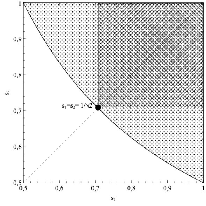
Eq. (42) defines the domain of genuine entanglement of the state (the whole shaded area above the graph depicted on Fig. 10). In particular, we can specify the maximal square subdomain (also shown on Fig. 10)
| (43) |
where the parameters and vary independently and where this state is GE. With the use of Eq. (40), this region can be rewritten in terms of . For we obtain
| (44) |
which extends the domain in Eq. (36). For larger the region becomes even wider:
| (45) |
with the upper bound tending to , when .
IV.2 Construction of multipartite NPT and distillable subspaces
An important aspect in the tasks of quantum information processing is the possibility to extract pure entangled states from mixed ones. The states from which pure entanglement can be obtained are called distillable Bennett et al. 1996.
More formally, a state on is -distillable (or one-copy distillable) DiVincenzo et al. 2000 if there exists a pure Schmidt rank bipartite state such that
| (48) |
where – the transpose operation applied on subsystem (the partial transpose). Next, a state is -distillable if is -distillable.
All distillable states are necessarily NPT - those with partial transpose having at least one negative eigenvalue (non-positive partial transpose). It is an open question whether the converse is true.
A multipartite subspace is called NPT with respect to some bipartite cut if any density operator with support in the subspace is NPT across this bipartite cut. Such subspaces can serve as a source of various mixed NPT states that could potentially be distillable. There are several known constructions of multipartite subspaces that are NPT with respect to certain bipartite cuts Sengupta et al. 2014; Johnston et al. 2019. In particular, Ref. Johnston et al. 2019 provides the method of construction of maximal multipartite subspaces that are NPT across at least one bipartite cut.
In this subsection we show that -partite subspaces that are NPT with respect to any bipartite cut can be constructed from bipartite NPT subspaces. We call a multipartite subspace -distillable across some bipartite cut if any density operator supported on the subspace is -distillable across this cut.
Lemma 6.
Let be a system of bipartite NPT subspaces of tensor product Hilbert spaces , respectively (). Let
be a subspace of an -partite tensor product Hilbert space , after taking tensor products and joining subsystems and , and , …, and into , , …, , respectively. Then is NPT across any bipartite cut. If, in addition, each of bipartite subspaces is -distillable, then is -distillable across any bipartite cut.
See Appendix A for the proof.
Example: construction of a tripartite subspace -distillable across any bipartite cut
We construct this example from tensor product of two -distillable bipartite subspaces. To find such bipartite subspaces, we use the argument from Ref. Agrawal et al. 2019 which combines the results of Refs. Johnston 2013; Chen and Dokovic 2016. In Ref. Johnston 2013 it was shown that for a bipartite system NPT subspaces of dimension up to can be constructed. The NPT subspace of maximal dimension reads as
| (49) |
(Theorem 1 of Ref. Johnston 2013).
Next, in Ref. Chen and Dokovic 2016 it was shown that any rank 4 NPT state is -distillable, which, combined with the results of Ref. Chen and Djokovic 2011, means that all NPT states of rank at most 4 are -distillable. Therefore, bipartite subspaces (49) of dimensions up to are -distillable.
Using the above facts, we can take a subspace of Eq. (49) with , such that . Let denote a subspace obtained from the tensor product of with itself, with subsequent joining the two adjacent subsystems. is hence a -dimensional subspace of a tripartite Hilbert space. According to Lemma 6, is -distillable across any of the three bipartite cuts.
The subspace is spanned by the system of vectors obtained from all possible tensor products of vectors from with each other. After taking the tensor products the two adjacent subsystems are to be joined according to the lexicographic order:
| (50) |
or, more generally,
| (51) |
The tensor product of two vectors from (49)
| (52) |
indexed by and respectively, yields, by Eq. (51), a generic vector from the system of vectors spanning :
| (53) |
IV.3 Entanglement criterion
Corollary 4.1 can be combined with some known results to give entanglement conditions for mixed states supported on tensor products. We give one such example using the result of Ref. Demianowicz et al. 2021, a simple sufficient condition for a subspace to be completely entangled:
Theorem 1 (Ref. Demianowicz et al. 2021).
Let be a subspace spanned by pairwise orthogonal pure bipartite states such that
| (54) |
where – the geometric measure of entanglement. Then is a completely entangled subspace.
Combining it with Corollary 4.1, we obtain some sort of an entanglement criterion.
Lemma 7.
Let be a density operator on a tripartite tensor product Hilbert space , where each state is obtained from tensor product of pure states and , with subsequent joining subsystems and into . Suppose that each is entangled. Suppose that are mutually orthogonal and such that
Then is a genuinely entangled state.
V Discussion
We have presented several properties of genuinely entangled subspaces obtained from the tensor product structure.
The advantage of such a construction is the possibility to control such useful characteristics of states supported on the output GESs as various measures of entanglement, distillability across some or all bipartite cuts, robustness of entanglement under mixing with external noise (not covered here, but it easily follows from Eqs. (68)-(71) of Ref. Antipin 2021). In particular, highly entangled subspaces can be generated in this way. In addition, if a tripartite GES is constructed from two CESs with given geometric measures of entanglement, and one of them corresponds to an entanglement breaking channel, then, according to Remark on page Remark, the exact values of the geometric measure across all three bipartite cuts are known for the resulting GES.
It has also been shown that, under certain conditions, GESs can be obtained from the direct sum of tensor products of bipartite CESs (Lemma 4). Such a structure reminds of the inner product of vectors in the Euclidean space, although here in Lemma 4 the conditions are not symmetric with respect to the left and the right subspaces in tensor products. In addition, as it was shown in Ref. Antipin 2021, the scheme of Fig. 2, used in the proof of the lemma, cannot generate GESs of maximal possible dimensions, although the dimensions of output GESs asymptotically approach the maximal ones when local dimensions of subsystems are high. Therefore, the construction of Lemma 4 doesn’t generate maximal GESs either. A possible direction of further research can be the generalization of Lemma 4 with the aim to obtain more symmetric conditions on bipartite subspaces as well as conditions sufficient for construction of maximal GESs.
Acknowledgements.
The author thanks M. V. Lomonosov Moscow State University for supporting this work.Appendix A Proof of Lemma 6
Proof.
We prove the lemma for , the case of arbitrary can be considered in a similar way.
Let be a density operator supported on , where (we use and interchangeably), so that has an ensemble decomposition
| (55) |
with being decomposed as
| (56) |
where , , and .
For the bipartite cut we choose the partial transpose to act on subsystem . We want to show that there is a pure state such that
| (57) |
We can take to have structure
| (58) |
(before joining and ), with some pure states , . Now, for each term in decomposition (55), it can be noted that in expression
| (59) |
the operations and scalar product with can be taken independently (as acting on different subsystems). So, first taking a partial scalar product of with , with the use of Eq. (56) we obtain
| (60) |
where – some normalized state from the subspace and – the corresponding normalization constant. Now the left part of Eq. (57) can be written as
| (61) |
where
| (62) |
a state entirely supported on , with
| (63) |
Since the state is NPT, choosing in Eq. (58) the state such that
| (64) |
we obtain the state for which condition (57) is satisfied, and this shows that is NPT across bipartite cut .

The reasoning in Eqs. (59)-(62) can be conveniently represented diagrammatically, as shown on Fig. 11.
If, in addition, subspace is -distillable, then there exists a Schmidt rank state such that condition (64) is satisfied. Using this state in Eq. (58), we construct a Schmidt rank state (again, after joining and ) such that condition (57) is satisfied, thus proving -distillability of across bipartite cut .
The same holds for bipartite cut (subspaces and enter the lemma symmetrically).
Consider now bipartite cut . This time we choose the partial transpose to act on joint subsystem . This operation reduces to taking transposes on subsystems and independently: .
For the state we can take the structure (58) requiring the state to be a product state:
| (65) |
with some pure states and .
Now, for each term in Eq. (55), the partial scalar product of with the transposed projector can be written as
| (66) |
where we took advantage of the product structure (65) to eliminate the second transpose operation (see also Fig. 12). Here denotes the vector with components equal to complex conjugated components of the vector with respect to the computational basis.

Now it can be easily seen that this case is reduced to the previous one of bipartite cut with the state replaced with : we can repeat the reasoning starting from Eq. (59) on and obtain that is NPT across bipartite cut . If, in addition, subspace is -distillable, then is -distillable across .
When , each possible bipartite cut can be analyzed similarly: choosing appropriate product structure of the state , we reduce the case with many transposes acting on different subsystems to the situation where there is only one partial transpose acting on some state that is entirely supported on one of the subspaces , then repeat the above reasoning. ∎
References
- Parthasarathy (2004) K. R. Parthasarathy, Proc. Math. Sci. 114, 365 (2004).
- Demianowicz and Augusiak (2018) M. Demianowicz and R. Augusiak, Phys. Rev. A 98, 012313 (2018).
- Cubitt et al. (2008) T. Cubitt, A. Montanaro, and A. Winter, J. Math. Phys. 49, 022107 (2008).
- Yeo and Chua (2006) Y. Yeo and W. K. Chua, Phys. Rev. Lett. 96, 060502 (2006).
- Muralidharan and Panigrahi (2008) S. Muralidharan and P. K. Panigrahi, Phys. Rev. A 77, 032321 (2008).
- Yamasaki et al. (2018) H. Yamasaki, A. Pirker, M. Murao, W. Dür, and B. Kraus, Phys. Rev. A 98, 052313 (2018).
- Demianowicz and Augusiak (2019) M. Demianowicz and R. Augusiak, Phys. Rev. A 100, 062318 (2019).
- Antipin (2021) K. V. Antipin, J. Phys. A: Math. Theor. 54, 505303 (2021).
- Shenoy and Srikanth (2019) A. Shenoy and R. Srikanth, J. Phys. A: Math. Theor. 52, 095302 (2019).
- Huber and Grassl (2020) F. Huber and M. Grassl, Quantum 4, 284 (2020).
- Agrawal et al. (2019) S. Agrawal, S. Halder, and M. Banik, Phys. Rev. A 99, 032335 (2019).
- Demianowicz and Augusiak (2020) M. Demianowicz and R. Augusiak, Quantum Information Processing 19, 199 (2020).
- Demianowicz (2021) M. Demianowicz, Universal construction of genuinely entangled subspaces of any size, arXiv preprint arXiv:2111.10193 (2021).
- Simon (2017) C. Simon, Nat. Phot. 11, 678 (2017).
- Biamonte et al. (2019) J. Biamonte, M. Faccin, and M. D. Domenico, Commun. Phys. 2, 53 (2019).
- Kraft et al. (2021) T. Kraft, C. Spee, X.-D. Yu, and O.Gühne, Phys. Rev. A 103, 052405 (2021).
- Contreras-Tejada et al. (2022) P. Contreras-Tejada, C. Palazuelos, and J. I. de Vicente, Phys. Rev. Lett. 128, 220501 (2022).
- Dai et al. (2020) Y. Dai, Y. Dong, Z. Xu, W. You, C. Zhang, and O.Gühne, Phys. Rev. Applied 13, 054022 (2020).
- Wilde (2013) M. M. Wilde, Quantum Information Theory (Cambridge University Press, 2013).
- Aubrun and Szarek (2017)
G. Aubrun and S. J. Szarek, Alice and Bob Meet
Banach:
The Interface of Asymptotic Geometric Analysis and Quantum Information Theory (American Mathematical Society, 2017). - Devetak and Shor (2005) I. Devetak and P. Shor, Comm. in Math. Phys. 256, 287 (2005).
- Stinespring (1955) W. F. Stinespring, Proc. Amer. Math. Soc. 6, 211 (1955).
- Coecke and Kissinger (2017) B. Coecke and A. Kissinger, Picturing Quantum Processes. A First Course in Quantum Theory and Diagrammatic Reasoning (Cambridge University Press, 2017).
- Wood et al. (2015) C. J. Wood, J. D. Biamonte, and D. G. Cory, Quant. Inf. Comp. 15, 0579 (2015).
- Biamonte (2019) J. D. Biamonte, Lectures on quantum tensor networks, arXiv preprint arXiv:1912.10049 (2019).
- Amosov et al. (2000) G. G. Amosov, A. S. Holevo, and R. F. Werner, Problems Inform. Transmission 36, 305 (2000).
- Werner and Holevo (2002) R. Werner and A. Holevo, J. Math. Phys. 43, 4353 (2002).
- King (2003) C. King, Quantum Information and Computation 3, 186 (2003).
- Hayden and Winter (2008) P. Hayden and A. Winter, Commun. Math. Phys. 284, 263 (2008).
- Shen and Chen (2020) Y. Shen and L. Chen, J. Phys. A: Math. Theor. 53, 125302 (2020).
- Sun and Chen (2021) Y. Sun and L. Chen, Ann. Phys. (Berlin) 533, 2000432 (2021).
- Vidal et al. (2002) G. Vidal, W. Dür, and J. I. Cirac, Phys. Rev. Lett. 89, 027901 (2002).
- Antipin (2020) K. V. Antipin, Mod. Phys. Lett. A. 35, 2050254 (2020).
- Bennett et al. (1996) C. H. Bennett, D. P. DiVincenzo, J. A. Smolin, and W. K. Wootters, Phys. Rev. A 54, 3824 (1996).
- DiVincenzo et al. (2000) D. P. DiVincenzo, P. W. Shor, J. A. Smolin, B. M. Terhal, and A. V. Thapliyal, Phys. Rev. A 61, 062312 (2000).
- Sengupta et al. (2014) R. Sengupta, Arvind, and A. I. Singh, Phys. Rev. A 90, 062323 (2014).
- Johnston et al. (2019) N. Johnston, B. Lovitz, and D. Puzzuoli, Quantum 3, 172 (2019).
- Johnston (2013) N. Johnston, Phys. Rev. A 87, 064302 (2013).
- Chen and Dokovic (2016) L. Chen and D. Z. Dokovic, Phys. Rev. A 94, 052318 (2016).
- Chen and Djokovic (2011) L. Chen and D. Z. Djokovic, J. Phys. A: Math. Theor. 44, 285303 (2011).
- Demianowicz et al. (2021) M. Demianowicz, G. Rajchel-Mieldzioc, and R. Augusiak, New J. Phys. 23, 103016 (2021).
*