Summarising and Comparing Agent Dynamics
with Contrastive Spatiotemporal Abstraction

According to several influential theories Hesslow, 1988; Van Fraassen, 1988; Lipton, 1990, explanations are constructed by searching for contrasts with alternative cases. This in turn implies that a common representation of multiple phenomena has explanatory value to the extent that it preserves information about their mutual differences, while ignoring irrelevant details. Motivated by this reasoning, we propose that a useful abstraction $\mathcal{X}$ is compact (small $m$) while nonetheless maximising our ability to discriminate between chains $i\in\{1,...,k\}$ based on their abstract transition probabilities. This is practically facilitated by placing the boundaries of abstract states at points of divergence between the chains, thus disentangling their transitions.

Let us consider the sequence of abstract models, defined by the joint probabilities $J^{\mathcal{X}}_{1},...,J^{\mathcal{X}}_{k}$, as generative distributions from which abstract transitions can be sampled. Applying Bayes’ rule, the posterior probability of a chain $i$ given a transition $x,x^{\prime}$ sampled from its abstract model is

where the vector $\rho\in[0,1]^{k}$, $\sum_{i=1}^{k}\rho_{i}=1$ specifies a prior weighting over chains. Taking the prior-weighted expectation of the log posterior over all chains and transitions, we obtain:

$\mathcal{H}$ is entropy, and JSD denotes the multi-distribution generalisation of the Jensen-Shannon divergence Lin, 1991, which is equivalent to the mutual information between the prior-weighted mixture distribution $\sum_{i=1}^{k}\rho_{i}J^{\mathcal{X}}_{i}$ and the indicator variable $i$. Intuitively, Equation 3 tells us that chain discrimination is facilitated by an abstraction that yields abstract transition probabilities $J^{\mathcal{X}}_{1},...,J^{\mathcal{X}}_{k}$ which are as mutually-divergent as possible, and also by minimising $\mathcal{H}(\rho)$, although this second term is not relevant here since we take $\rho$ to be a fixed parameter specifying our level of interest in each chain.

We therefore propose the following contrastive abstraction objective. Given a set of state abstractions $\mathbb{X}$ constructible by some well-defined algorithm, the objective is

Here, $\mathcal{H}(\rho)$ is ignored because it is independent of $\mathcal{X}$, and the second term (parameterised by $\alpha>0$) is a complexity regulariser to incentivise smaller abstractions. This term is required to ensure the objective is not maximised by the trivial solution $\mathcal{X}=\mathcal{S}$. In expectation, the JSD term increases monotonically but sublinearly with $m$ (see Appendix A for a simple theoretical analysis and empirical demonstration), and $\alpha(m-1)$ is evidently linear, so we should expect their difference to be maximised at an intermediate abstraction size determined by $\alpha$ (larger $\alpha$ favours smaller $m$).

The preceding discussion concerns a $k$-chain sequence $\mathcal{P}=(P_{1},...,P_{k})$. A special case of this setup is when the sequence is the product of a contiguous, temporally-evolving process: a nonstationary Markov chain. Suppose that $k$ is very large, and that the dataset $\mathcal{D}$ contains a small number of samples from each $P_{i}$ (perhaps as few as $1$). Regardless of our choice of state abstraction $\mathcal{X}$, the result will be an array of joint probabilities $J^{\mathcal{X}}$ that is not only large (hampering interpretability) but also sparse, meaning the abstract Markov chains will have such high variance as to be practically useless as models of $\mathcal{P}$.

In many real-world dynamical systems, however, changes are incremental, so it is reasonable to assume approximate stationarity over short timescales. We therefore propose to reduce both the size and the sparsity of $J^{\mathcal{X}}$ by applying a second layer of temporal abstraction, which approximates the dynamics as piecewise constant within $n\ll k$ disjoint and exhaustive temporal windows $\mathcal{T}=\{\tau_{1},...,\tau_{n}\}$, where each $\tau_{w}$ is parameterised by lower and upper bounds $l_{w},u_{w}$, and the following constraints hold: $l_{1}=1$; $u_{n}=k+1$; $l_{w}<u_{w},\ \forall w\in\{1,...,n\}$; $u_{w}=l_{w+1},\ \forall w\in\{1,...,n-1\}$. These can be used to aggregate $J^{\mathcal{X}}$ along its first axis to form a smaller and less sparse $n\times m\times m$ array $J^{\mathcal{X},\mathcal{T}}$, where $\forall w\in\{1,...,n\},x\in\mathcal{X},x^{\prime}\in\mathcal{X}$,

and $\rho^{\mathcal{T}}_{w}=\sum_{i=l_{w}}^{u_{w}-1}\rho_{i}$ aggregates the elements of the prior vector for each window. By varying both $n$ and the window boundaries in $\mathcal{T}$, we obtain different sequences of spatiotemporally-abstracted transition probabilities, even if $\mathcal{X}$ remains constant. Intuitively, a temporal abstraction is informative for contrastive analysis if it contains windows of behaviour which are internally consistent, but between which there are significant differences. We suggest that this can be achieved using an identical objective to that of the previous section: maximising the Jensen-Shannon divergence between the joint transition distributions of the windows. We again wish to incentivise compact temporal abstractions (small $n$), so add another regularisation term to the objective:

where $\mathbb{T}$ is the set of temporal abstractions constructible by some algorithm, and $\beta>0$ is a hyperparameter. Theoretical and empirical results again indicate that JSD is sublinear in $n$ (Appendix A). As with $m$, this means that the objective will be maximised at a finite value of $n$ determined by $\beta$.

Suppose we have an existing abstraction $\mathcal{X}$, consisting of $m$ hyperrectangles in the state space $\mathcal{S}=\mathbb{R}^{D}$, and have precomputed the joint abstract transition probabilities $J^{\mathcal{X}}$ by equation 1 and normalisation. Now consider splitting an abstract state $x\in\mathcal{X}$ into two by placing a hyperplane at a location $c\in\mathbb{R}$ along state dimension $d\in\{1,...,D\}$. All transitions into, out of and within the abstract state will be redistributed between the two “child” abstract states. This can be represented by an enlarged transition array with shape $k\times(m+1)\times(m+1)$, denoted by $J^{\mathcal{X}\rightarrow[xdc]}$. The splitting operation increases the quality of the abstraction according to the objective in equation 4 by an amount equal to the increase in JSD (always $+$ve), minus the regularisation parameter $\alpha$:

The CSA algorithm initiates with one abstract state covering the entire space, $\mathcal{X}=\{\mathcal{S}\}$. It then proceeds to recursively partition the space into ever-smaller hyperrectangles, at each step selecting $x$, $d$ and $c$ to greedily maximise equation 7:

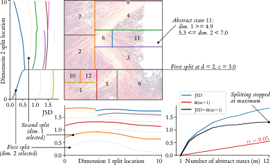
$\mathcal{C}_{d}$ is a finite set of candidate split thresholds along dimension $d$, defined either manually or using the data (e.g. all values occurring in $\mathcal{D}$). The algorithm terminates when all possible $\delta$ values are $\leq 0$, which occurs earlier for larger values of $\alpha$. Figure 2 provides an example of the algorithm in operation.

The first step in this extended algorithm is to apply an initial temporal abstraction $\mathcal{T}_{\text{init}}$, which should be chosen to reduce the sparsity of $J^{\mathcal{X},\mathcal{T}_{\text{init}}}$ to an acceptable level, but to otherwise have as many windows as possible to avoid excessive smoothing of the nonstationary dynamics (if sparsity is not an issue, the null abstraction $\mathcal{T}_{\text{null}}=\{[1\leq i<2],...,[k\leq i<k+1]\}$ can be used). After applying the initial temporal abstraction, CSA is called as a subroutine, yielding a state abstraction $\mathcal{X}$ that maximises the JSD between the initial windows.

We then run a secondary stage of temporal partitioning to find another set of windows $\mathcal{T}$ (typically $|\mathcal{T}|\ll|\mathcal{T}_{\text{init}}|$) that preserve JSD as much as possible. This is also a recursive procedure. Given an existing $\mathcal{T}$ consisting of $n$ windows, splitting the $w\in\{1,...,n\}$th window at a location $i\in\{2,...,k\}$ creates two child windows with respective boundaries $l_{w},i$ and $i,u_{w}$. This yields an enlarged transition array with shape $(n+1)\times m\times m$, denoted by $J^{\mathcal{X},\mathcal{T}\rightarrow[wi]}$.

Initiating with one window covering the entire chain sequence, $\mathcal{T}=\{[1\leq i<k+1]\}$, CSTA iteratively adds windows by splitting, at each step selecting $w$ and $i$ to greedily maximise performance according to equation 6:

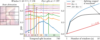
and $\mathcal{C}_{\text{temporal}}$ is a finite set of candidate temporal split thresholds. In our implementation, we exclude from $\mathcal{C}_{\text{temporal}}$ any threshold that would violate a minimum window width $\varepsilon$. The algorithm terminates as soon as either this condition leaves no valid thresholds, or all possible $\delta$ values are $\leq 0$, the latter of which occurs earlier for larger values of $\beta$. Algorithm 2 contains pseudocode for CSTA, and Figure 3 provides an example of the temporal partitioning stage.

In this MDP, shown in (a), the agent controls the position $s=[x,y]\in[0,10]^{2}$ of a marker via its velocity $a\in[-.25,.25]^{2}$. It attains $+100$ reward for reaching a goal and $-100$ for entering a penalty region, and walls at $y=3$ and $y=7$ block transverse motion. Episodes terminate on entering the goal or penalty, or after $200$ timesteps. The RL algorithm has the objective of maximising reward, so converges over $k=750$ episodes to a policy that moves to the goal while avoiding the walls, as shown in the transition data plot (b). Figure 2 uses this dataset, and shows that our algorithm makes its first and third splits at $y=3$ and $y=7$ respectively, which align exactly with the walls. The sharp peaks in JSD around these locations, visible in the left sub-plot, suggest that this is no coincidence, and that the changing ability of the agent to pass each wall is a major source of divergence in the policy sequence. Other splits have similarly intuitive origins, with abstract states $6$ and $8$ respectively covering a critical junction at the upper wall where the agent has to learn a sharp right turn, and part of the upper maze boundary along which the agent learns to “slide” to the goal near the end of learning. Returning to Figure 1, (e) provides an alternative visualisation of the state abstraction as a tree diagram, showing how the $m=12$ abstract states are hierarchically defined by the splits.

The temporal abstraction stage, whose details are the subject of Figure 3, yields $n=10$ windows, which are overlaid on the agent’s learning curve (mean reward over a $10$-episode radius) in Figure 1 (d). Notice the alignment between the window boundaries and various jumps and direction changes in the learning curve; this provides encouragement that the JSD-based split criterion is effective for partitioning learning into periods of qualitatively similar behaviour.

For windows $3$ and $10$, we examine the abstract state dynamics in detail using transition graphs in Figure 1 (f), where node/edge opacities scale with state visitation and joint transition probabilities respectively. From these, we can derive contrastive interpretations of the agent’s learning, such as:

• •

  The sparser and less symmetric graph for window $10$ indicates a general trend towards goal-directed behaviour.

• •

  Transitions providing progress to the goal (e.g. $3\rightarrow 6$) become more common, while those leading to corners or dead-ends (e.g. $9\rightarrow 5$) occur less frequently.

• •

  Abstract state $1$ sees both a decrease in visitation and a focusing of outbound transitions to state $5$ only. Inbound transitions to state $1$ disappear entirely; in window $10$, the agent only visits the state if initialised there.

Stacked bar charts in Figure 1 (g, h) give a complementary view on the changing dynamics across all windows. In (g), bar heights reflect the marginal visitation distribution, and in (h) they represent the conditional outbound probabilities from abstract state $6$ only. They provide further contrastive insight:

• •

  Initially approximately uniform, marginal visitation gradually skews towards abstract state $4$ and away from $2,7$ and $9$. Visits to state $3$ remain largely unchanged.

• •

  Aberrations include two “waves” of visitation to state $1$, in which the agent fails to exit the bottom-left corner.

• •

  The outbound $6\rightarrow 4$ transition comes to dominate, indicating a learnt ability to turn past the upper wall.

• •

  The $6\rightarrow 11$ transition briefly spikes in window $6$; at this time the agent often becomes stuck below the wall.

In this MDP, Figure 4 (a), the agent uses two thrusters to land a craft between flags, with $\pm 100$ reward for landing/crashing, and shaping reward promoting smooth flight. Episodes end on landing/crashing, or after $400$ timesteps. To sense-check the temporal abstraction, we run a random policy for $250$ episodes then enable the RL algorithm for a further $250$.

Contrastive spatiotemporal abstraction yields $12$ abstract states (b) and $6$ time windows (c). The inherent symmetry of the MDP is reflected in splits along the horizontal state dimension $x$, with the first close to the centreline and others near $\pm 0.1$ and $\pm 0.2$ (note: flags are at $\pm 0.2$). $8$ out of $11$ splits concern the agent’s behaviour in $x$ (including velocity $v^{x}$), suggesting most temporal contrasts occur along this dimension: vertical dynamics are largely gravity-driven, thus remain constant over learning. Exceptions are the splits along $y$ to create abstract states $2$ and $5$, corresponding to being low and central (i.e. correct landing) on the right/left respectively. These and other linguistic labels are given in a semantic key (d), which aids us in interpreting abstract state dynamics.

Turning to the temporal abstraction (c), we see that all splits lie in the RL phase, before the agent converges to a stable reward of $\approx 150$. This passes the aforementioned sense-check, and aligns with theory: JSD is maximised by splitting at times when transition probabilities are changing; splitting a stationary window gives zero JSD gain in expectation.

(e) shows marginal abstract state visitation. In window $1$ most time is spent drifting out from the centre (states $3,4$) but this is rapidly unlearnt. Visits to the landing states $2,5$ increase; others oscillate in prevalence before convergence.

A richer narrative emerges from the transition graphs for all six windows (f). We focus on states on the left of the state space, enclosed in dotted lines. The trends are complex and nonlinear, as expected from a stochastic learning agent, but our annotations tell the story of over-rotated leftward motion in state $3$ giving way to a slower leftward drift $10\rightarrow 7\rightarrow 1$, punctuated by a brief abandonment of left-side approaches, and finally a convergence to landing state $5$ with a preference for arced approaches via states $1$ and $7$. Such insight would typically require a laborious review of the learning history, but is automatically mined by contrastive abstraction.

The preceding interpretation is reinforced by visualising the prototype episode (g) for each window $w$, that which is most representative of the window’s dynamics according to the mean log likelihood over the conditional transition distribution: $\text{argmax}_{l_{w}\leq i<u_{w}}[\frac{1}{\text{len}(i)}\sum_{t=0}^{\text{len}(i)-1}\log P^{\mathcal{X},\mathcal{T}}_{w,x_{i,t},x_{i,t+1}}]$. In Appendix D we show how a similar calculation allows us to dynamically assess the representativeness of an ongoing episode with respect to each window, and in turn provides a mechanism for counterfactual review of critical transitions.

For reference, the form of the Jensen-Shannon divergence given in the main paper is

which can be expanded as follows:

Consider the scaling of JSD with $m$ under a binary partition operation, which involves replacing a randomly-selected abstract state $x_{0}\in\mathcal{X}$ with two others $x_{1}$ and $x_{2}$, subject to the following conservation equations for all $i\in\{1,...,k\}$:

where $\mathcal{X}^{-}$ denotes all abstract states except $x_{0}$, $x_{1}$ and $x_{2}$ themselves, and we have dropped the superscripted $\mathcal{X}$ from $J^{\mathcal{X}}_{\cdot,\cdot,\cdot}$ to reduce visual clutter. All other transition probabilities (i.e. between the members of $\mathcal{X}^{-}$) remain unchanged. This scaling analysis is of interest because the algorithm presented in Section 3 of the main paper employs a binary partitioning approach.

Let $\delta_{\text{JSD}}$ denote the difference between the JSD values before and after the partition is made. Most terms of this difference cancel, and we are left with

where

A general analysis of $\delta_{\text{JSD}}$ is not straightforward, so here we only consider the special case of $k=2$ Markov chains with prior weighting $\rho_{1}=\rho_{2}=\frac{1}{2}$. As a lower bound, if the underlying state transition probabilities in $\mathcal{S}$ are identical for chains $1$ and $2$, it is easy to show that all terms cancel and $\delta_{\text{JSD}}=0$. More interestingly, we can upper bound the JSD difference by considering the “perfect partitioning” case when chains $1$ and $2$ have the same inbound and outbound transition probabilities for $x_{0}$ (i.e. $J_{1,x_{p},x_{0}}=J_{2,x_{p},x_{0}}$ and $J_{1,x_{0},x_{p}}=J_{2,x_{0},x_{p}}$, $\forall x_{p}\in\mathcal{X}^{-}\cup\{x_{0}\}$), but chain $1$ only visits $x_{1}$ and chain $2$ only visits $x_{2}$. This leads to the following simplification of the terms $z_{p,1}+z_{p,2}-z_{p,0}$ for each $x_{p}\in\mathcal{X}^{-}$:

where the subscripted placeholder “$\cdot$” indicates that this joint probability is the same for both chains. An equivalent simplification can be derived for $z_{1,p}+z_{2,p}-z_{0,p}$, and also for $z_{1,1}+z_{2,2}-z_{0,0}$. We also know that $z_{1,2}=z_{2,1}=0$, because (by assumption) neither of the two chains ever visits both $x_{1}$ and $x_{2}$. Substituting back into the equation for $\delta_{\text{JSD}}$, we have

where $M_{\cdot,x_{0}}=\sum_{x_{p}\in\mathcal{X}}J_{\cdot,x_{0},x_{p}}$ is the marginal visitation probability for $x_{0}$, obtained by summing over all joint outbound transition probabilities. This quantity is the same for both chains.

What can we say about the behaviour of $\delta_{\text{JSD}}$ in expectation? For any Markov chain $i$, $\sum_{x\in\mathcal{X}}M_{i,x}=1$, so if $x_{0}$ was selected for partitioning with uniform random probability, $\mathbb{E}_{x_{0}}[M_{\cdot,x_{0}}]=\frac{1}{m}$ (where $m$ is the number of abstract states before the partition is made). We can also bring the expectation of the second term inside the sum:

We cannot say much more about the second term in general, aside from that it will depend on the amount of “inertia” in the Markov chains: the proportion of timesteps in which they remain in the same abstract state as opposed to transitioning elsewhere. If inertia is very high, the first term of our expression for $\mathbb{E}_{x_{0}}[\delta_{\text{JSD}}]$ will dominate, in which case

since $\frac{d}{dy}(a\log y)=\frac{a}{y}$. This result suggests that in the high-inertia context, JSD is approximately logarithmic in $m$. Finally, as a looser upper bound, we can say for certain that $J_{\cdot,x_{p},x_{0}}\leq M_{\cdot,x_{p}}$, so $\mathbb{E}_{x_{0}}[J_{\cdot,x_{p},x_{0}}]\leq\frac{1}{m},\ \forall x_{p}\in\mathcal{X}^{-}$. Therefore,

since $\frac{d}{dy}(ay)=a$. In this (extremely generous) upper bound case, JSD is linear in $m$. As this case will be realised very rarely in practice, it is reasonable to say that the scaling will almost always be sublinear, and more tentatively, that it is approximately logarithmic.

A more general analysis is possible for $n$. When temporal abstraction is applied to aggregate $k$ temporally-ordered Markov chains into $n$ windows, the Jensen-Shannon divergence is given by

Consider the replacement of a randomly-selected time window $w_{0}\in\{1,...,n\}$ with two others $w_{1}$ and $w_{2}$, subject to the following conservation equations for all $x\in\mathcal{X},x^{\prime}\in\mathcal{X}$:

where we have dropped the superscripted $\mathcal{X}$ and $\mathcal{T}$ from both $\rho^{\mathcal{T}}$ and $J^{\mathcal{X},\mathcal{T}}_{\cdot,\cdot,\cdot}$ to reduce visual clutter. Note that this form of conservation results from partitioning a window in two.

Again taking $\delta_{\text{JSD}}$ to be the difference between the JSD values before and after the partitioning, all of the second term (of the form given above), and most components of the first term, cancel out. We are left with

Applying the conservation equations and multiplying and dividing by $\rho_{w_{0}}$, we can rewrite this as

By inspection, everything aside from the leading $\rho_{w_{0}}$ exactly matches the definition of the JSD itself, calculated pairwise between windows $w_{1}$ and $w_{2}$, and using renormalised weights:

$\delta_{\text{JSD}}$ is lower-bounded by zero in the case when $w_{1}$ and $w_{2}$ have identical transition probabilities in $\mathcal{X}$ (since pairwise JSD will be zero). As an upper bound, we again consider a “perfect partitioning” case where the two new windows have no abstract state transitions in common (i.e. $J_{w_{1},x,x^{\prime}}>0\implies J_{w_{2},x,x^{\prime}}=0$ and $J_{w_{2},x,x^{\prime}}>0\implies J_{w_{1},x,x^{\prime}}=0$, $\forall x\in\mathcal{X},x^{\prime}\in\mathcal{X}$), and equal prior weighting $\rho_{w_{1}}=\rho_{w_{2}}=\frac{\rho_{w_{0}}}{2}$. Returning to the expanded form of $\delta_{\text{JSD}}$ and substituting in these relations, we obtain

where the subscripted placeholder “$\cdot$” now stands for either $w_{1}$ or $w_{2}$; whichever of the two has nonzero transition probability for each $x,x^{\prime}$ pair. In the final line above, the double sum cancels to $2$ because for each of the two windows, the sum of joint probabilities is $1$.

Finally, we know that $\sum_{w=1}^{n}\rho_{w}=1$, so if we assume that $w_{0}$ was selected uniform-randomly, $\mathbb{E}_{w_{0}}[\rho_{w_{0}}]=\frac{1}{n}$ (where $n$ is the number of chains before the partition is made). Therefore,

since $\frac{d}{dy}(a\log y)=\frac{a}{y}$. We can thus conclude from this upper-bound analysis that JSD is reliably sublinear in $n$.

As a simple empirical validation of the preceding results, we generated datasets of $k=100$ random trajectories of length $T=100$ (one per “chain”) in the 2D region $\mathcal{S}=[0,1]^{2}$ according to a parameterised Gaussian random walk model:

The $\text{clip}(\cdot)$ function clips states into the $[0,1]^{2}$ region. In each trajectory, Gaussian noise with standard deviation $\sigma$ is added to a mean velocity vector with magnitude $v$, which is gradually rotated through $270^{\circ}$ over the sequence $i\in\{1,...,k\}$.

We generated four datasets with various arbitrarily-chosen values of $v$ and $\sigma$. For each dataset, we performed recursive axis-aligned partitioning of the region up to a maximum abstraction size $m$ and measured the resultant JSD. To select split points we used both a random strategy and the CSTA algorithm presented in Section 3 of the main paper, which greedily maximises the JSD gain on each step.

As predicted by the preceding theory, the scaling of JSD is consistently sublinear in both $m$ and $n$. It is also always higher when the CSTA algorithm is used, compared with random splitting. Note that these datasets have an extremely simple dynamical structure; the advantage of principled split selection using CSTA is likely to be far greater in practical applications.

References

- Adadi and Berrada, (2018) Adadi, A. and Berrada, M. (2018). Peeking inside the black-box: a survey on explainable artificial intelligence (xai). IEEE access, 6:52138–52160.
- Amir and Amir, (2018) Amir, D. and Amir, O. (2018). Highlights: Summarizing agent behavior to people. In Proceedings of the 17th International Conference on Autonomous Agents and MultiAgent Systems, pages 1168–1176. International Foundation for Autonomous Agents and Multiagent Systems.
- Bastani et al., (2018) Bastani, O., Pu, Y., and Solar-Lezama, A. (2018). Verifiable reinforcement learning via policy extraction. arXiv preprint arXiv:1805.08328.
- Bewley and Lawry, (2021) Bewley, T. and Lawry, J. (2021). TripleTree: A Versatile Interpretable Representation of Black Box Agents and their Environments. In Proceedings of the AAAI Conference on Artificial Intelligence.
- Brockman et al., (2016) Brockman, G., Cheung, V., Pettersson, L., Schneider, J., Schulman, J., Tang, J., and Zaremba, W. (2016). OpenAI Gym.
- Davoodi and Komeili, (2021) Davoodi, O. and Komeili, M. (2021). Feature-based interpretable reinforcement learning based on state-transition models. arXiv preprint arXiv:2105.07099.
- Haarnoja et al., (2018) Haarnoja, T., Zhou, A., Hartikainen, K., Tucker, G., Ha, S., Tan, J., Kumar, V., Zhu, H., Gupta, A., Abbeel, P., et al. (2018). Soft actor-critic algorithms and applications. arXiv preprint arXiv:1812.05905.
- Hesslow, (1988) Hesslow, G. (1988). The problem of causal selection. Contemporary science and natural explanation: Commonsense conceptions of causality, pages 11–32.
- Huang et al., (2019) Huang, S. H., Held, D., Abbeel, P., and Dragan, A. D. (2019). Enabling robots to communicate their objectives. Autonomous Robots, 43(2):309–326.
- Huber et al., (2019) Huber, T., Schiller, D., and André, E. (2019). Enhancing explainability of deep reinforcement learning through selective layer-wise relevance propagation. In Joint German/Austrian Conference on Artificial Intelligence (Künstliche Intelligenz), pages 188–202. Springer.
- Kemeny and Snell, (1976) Kemeny, J. G. and Snell, J. L. (1976). Finite Markov chains. Springer-Verlag, 2 edition.
- Lin, (1991) Lin, J. (1991). Divergence measures based on the shannon entropy. IEEE Transactions on Information theory, 37(1):145–151.
- Lipton, (1990) Lipton, P. (1990). Contrastive explanation. Royal Institute of Philosophy Supplements, 27:247–266.
- McCalmon et al., (2022) McCalmon, J., Le, T., Alqahtani, S., and Lee, D. (2022). Caps: Comprehensible abstract policy summaries for explaining reinforcement learning agents. In Proceedings of the 21st International Conference on Autonomous Agents and Multiagent Systems, pages 889–897.
- Miller, (2018) Miller, T. (2018). Contrastive explanation: A structural-model approach. arXiv preprint arXiv:1811.03163.
- Sutton and Barto, (2018) Sutton, R. S. and Barto, A. G. (2018). Reinforcement learning: An introduction. MIT press.
- Topin and Veloso, (2019) Topin, N. and Veloso, M. (2019). Generation of policy-level explanations for reinforcement learning. In Proceedings of the AAAI Conference on Artificial Intelligence, volume 33, pages 2514–2521.
- Van Fraassen, (1988) Van Fraassen, B. (1988). The pragmatic theory of explanation. Theories of Explanation, 8:135–155.
- Zahavy et al., (2016) Zahavy, T., Ben-Zrihem, N., and Mannor, S. (2016). Graying the black box: Understanding dqns. In International conference on machine learning, pages 1899–1908. PMLR.
APPENDIX A. SUBLINEARITY OF THE JENSEN-SHANNON DIVERGENCE WITH AND
Theoretical Analysis for