Cosmological global dynamical systems analysis
Abstract
We consider a dynamical systems formulation for models with an exponential scalar field and matter with a linear equation of state in a spatially flat and isotropic spacetime. In contrast to earlier work, which only considered linear hyperbolic fixed point analysis, we do a center manifold analysis of the non-hyperbolic fixed points associated with bifurcations. More importantly though, we construct monotonic functions and a Dulac function. Together with the complete local fixed point analysis this leads to proofs that describe the entire global dynamics of these models, thereby complementing previous local results in the literature.
1 Introduction
Dynamical systems and dynamical systems methods were introduced in cosmology in 1971 by Collins [1] who treated 2-dimensional dynamical systems while Bogoyavlensky and Novikov (1973) [2] used dynamical systems techniques for higher dimensional dynamical systems in cosmology. This early work has subsequently been followed up and extended by many researchers, see e.g. [3, 4, 5]. The first dynamical systems analysis involving a minimally coupled scalar field was given by Belinskiǐ and coworkers [6, 7, 8, 9] who used dynamical systems to explore inflation, primarily focusing on the potentials and . In 1987 Halliwell [10] treated an exponential scalar field potential in Friedmann-Lemaître-Robertson-Walker (FLRW) cosmology, where the scalar field and an exponential representation of the cosmological scale factor were used as dynamical systems variables, which resulted in an unbounded state space and thereby only a local state space description (see also Ratra and Peebles (1988) [11] for early work using dynamical systems for this case). The first global state space treatment of a scalar field with an exponential potential was done in Bianchi cosmology, which contains FLRW cosmology as a special case, by Coley et al. (1997) [12]. Notable is also the work by Foster (1998) [13] who analysed asymptotically exponential scalar field potentials. Finally, Copeland et al. (1998) [14] treated the spatially flat FLRW case with an exponential potential and a perfect fluid with a linear equation of state. This latter work, which used a reduced 2-dimensional compact and regular state space, gave a linear fixed point (critical point, equilibrium point) stability analysis for parameter values that yielded hyperbolic fixed points.11 1 All eigenvalues of a linearization of a dynamical system at a so-called hyperbolic fixed point have non-zero real parts, and hence such a fixed point has no center manifolds.
In this paper we will investigate the models Copeland et al. considered, but we will extend their local fixed point analysis to the bifurcation values of the relevant model parameters, which yield non-hyperbolic fixed points with one zero eigenvalue, thereby requiring center manifold analysis. More importantly though, even in the case of the hyperbolic fixed points a linear fixed point analysis in a 2-dimensional compact state space does not necessarily imply a complete asymptotic description; other asymptotic behaviour is possible, such as periodic orbits and heteroclinic cycles.22 2 A heteroclinic orbit is a solution trajectory that originates and ends at two different fixed points; a heteroclinic chain consists of a concatenation of heteroclinic orbits, where the ending fixed point of one heteroclinic orbit is the starting fixed point of the next one; a heteroclinic cycle is a closed heteroclinic chain. For an example and detailed discussion of a heteroclinic cycle arising from a scalar field potential in the spatially flat FLRW case, see Foster (1998) [15]. In this paper we fill these gaps in the proof for the asymptotic and global behaviour of models with an exponential scalar field potential and a perfect fluid with a linear equation of state.
We finally note two additional motivational points: First, a substantial fraction of scalar field potentials used to describe inflation or/and quintessence are asymptotically exponential when the scalar field or/and . A global description of the solution space of such models therefore requires a global understanding of the present models. Second, a key ingredient for several of the proofs in the present paper are monotonic functions, which are derived by using methods first developed by Uggla in ch. 10 in [3] and later generalized by Uggla and coworkers in [16] and [17]. The present results thereby serve as an illustration of the power of those methods.
2 Dynamical systems description and local fixed point analysis
2.1 Field equations
We consider a flat and isotropic FLRW spacetime,
| (1) |
where is the cosmological scale factor. The source consists of matter with an energy density and pressure , and a minimally coupled scalar field, , with a potential , which results in
| (2) |
The Einstein equations, the (non-linear) Klein-Gordon equation, and the energy conservation law for the fluid, are given by33 3 We use units such that and , where is the speed of light and is Newton’s gravitational constant. (see, e.g., [18] for a slightly different formulation of the equations)
| (3a) | ||||
| (3b) | ||||
| (3c) | ||||
| (3d) | ||||
| (3e) | ||||
where an overdot represents the derivative with respect to the cosmic time ; a barotropic equation of state for the perfect fluid yields ; the total energy density and pressure are given by
| (4) |
Equation (3b) is the (Landau–-) Raychaudhuri equation, while (3c) is the Gauss/Hamiltonian constraint (often referred to as the Friedmann equation in FLRW cosmology). Here we are going to consider an exponential potential and a perfect fluid with a linear equation of state, i.e.,
| (5) |
where and are constants; matter, radiation and a stiff perfect fluid correspond to , and , respectively.
2.2 Explicitly solvable cases
For an exponential potential and a perfect fluid with linear equation of state the equations are solvable for several values of and , as was shown implicitly by Uggla et al. (1995) [19] (use equations (2.23), (2.37), (4.98) and in Table III in [19]), where it was also demonstrated how to obtain explicit solutions in as simple form as possible.44 4 To the authors’ knowledge, all known explicit solutions for problems with hypersurface homogeneity, in general relativity and modified gravity theories, are obtainable, and in their simplest form, by using the mechanisms and methods in [19]. The solvable cases are:
| (6a) | ||||||||
| (6b) | ||||||||
| (6c) | ||||||||
where we recognize the first case, , as a constant potential and the second case, , as a stiff perfect fluid.55 5 The explicitly solvable case , was used in [18] to illustrate how explicit solutions can be situated in a dynamical systems context. A problem where either the scalar field potential, , or is zero yields a trivially solvable problem, see [19].
2.3 The dynamical system
To obtain a useful dynamical system, we introduce the following dimensionless bounded quantities66 6 The variable was first introduced by Coley et al. (1997) [12] and Copeland et al. (1998) [14] whose is . Since then, (or ) is often used to describe scalar fields in cosmology, see, e.g., Urena-Lopez (2012) [20], equation (2.3), Tsujikawa (2013) [21], equation (16) and Alho and Uggla (2015) [18], equation (8). The reason for using the notation for the kernel is because plays a similar role as Hubble-normalized shear, which is typically denoted with the kernel , see e.g. [3].
| (7a) | ||||
| (7b) | ||||
| (7c) | ||||
A ′ henceforth denotes the derivative with respect to -fold time
| (8) |
where , . The definition (8) implies that and when and , respectively.
Throughout we replace with by using that
| (9) |
where
| (10) |
is the deceleration parameter.
Using and inserting (5) and the definitions (7) into (3) results in the following coupled system for the state vector :
| (11a) | ||||
| (11b) | ||||
where
| (12a) | ||||
| (12b) | ||||
Restricting to , as we will do later, it follows that , where when and , while when , . Another quantity that is often used in the context of scalar field is , or, equivalently, , defined by and hence
| (13) |
We use (12a) in (11) to globally solve for , although note that
| (14) |
which follows from (12a) and (11). This equation and (11b) show that and form an invariant boundary of the state space , which, due to that the dynamical system (11) is completely regular, can be included in the state space analysis. This is essential since some of the asymptotics are associated with this boundary. We will refer to the orbits with , as interior orbits and orbits with or/and , as boundary orbits.
The present formulation can be viewed as a transformation of an original state space (alternatively, , since ) to . The equations for and , and , decouple from the dynamical system for . This reduced state space can be therefore be regarded as a projection of the state space .77 7 More precisely, the new variables result in a skew-product dynamical system where the base dynamics acts in while the fiber dynamics acts in , a notion that was introduced in [22]. The reason for the decoupling of and is due to the linear equation of state for the perfect fluid and that .88 8 The present system is closely connected to that of Copeland et al. (1998) [14] who used and as variables. We prefer to use the more physical variable rather than . Moreover, note that in contrast to , the unfortunately widely used is unsuitable for many more general potentials. For examples where is inappropriate and for proper choices of variables, see, e.g., [23, 24, 25, 26]. Since the decoupled equations can be solved by quadratures once and are obtained, the system for the state vector contains the essential information for the present problem.
2.4 Local hyperbolic fixed point analysis
The fixed points of the dynamical system (11) and the eigenvalues of the linearization at the fixed points are given in Table 1.
| Name | Eigenvalues | ||||
| 1 | 0 | ; | |||
| 0 | ; | ||||
| 0 | ; | ||||
| 0 | 1 | ; | |||
The names of the fixed points are motivated as follows: are the boundary ‘kinaton’ fixed points, due to that and and hence that , which characterizes kinaton evolution (a nomenclature introduced in [27]); with and is the de Sitter fixed point while , which exists when and yields power law acceleration when , due to that at ; the fixed point is referred to as the Friedmann-Lemaître fixed point (); finally is the scaling fixed point (scaling due that at , since this implies that the scalar field mimics the dynamics of the fluid, with a constant ratio between both energy densities).
Apart from the de Sitter fixed point , which exists when , each of the other fixed points correspond to a unique self-similar (i.e., the corresponding spacetime admits a homothetic Killing vector field) power law solution, invariant under constant conformal scalings. On the other hand, the de Sitter fixed point corresponds to a one-parameter set of solutions, parametrized by the dimensional constant .
Without loss of generality, we will assume that (if , make the change ). We also limit the range of so that where and yield bifurcations, which is not surprising since results in a cosmological constant while a stiff fluid equation of state, , corresponds to that the speed of sound is equal to that of light (also, recall that is an explicitly solvable case). The above eigenvalues then yield the stability properties given in Table 2.
| Name | Domain | Stability |
|---|---|---|
|
Unstable node when
Saddle point for | ||
| Unstable node | ||
|
Stable node when
Saddle point for | ||
| Saddle point | ||
|
Stable node when
Stable spiral for |
It follows that there are three disjoint parameter regions when , , determined by the two bifurcations at and , see Figure 1:
- I:
.
- II:
, .
- III:
.

The boundary of region I, where the stable fixed point is replaced with the stable fixed point is, as mentioned, completely solvable. The solution in the state space can be obtained as follows. In this case, due to that , the system (11) is invariant under . Hence can be replaced with . This results in a system that is identical to that for a source with three matter components: (i) a perfect fluid with , (ii) a stiff fluid, i.e., a perfect fluid with an equation of state (and hence ), and (iii) a cosmological constant, . This problem easily yields the solution
| (15) |
while and . The invariant subset , and hence , corresponds to having a perfect fluid with a linear equation of state and a cosmological constant, where yields the CDM model. For a visual representation of the orbit structure for the models, see Figure 2.
The bifurcation boundary between region I and II at corresponds to that enters the state space through and takes over as the stable sink when instead of , which is a stable sink in region I and a saddle with one orbit entering the interior of the state space in region II. The bifurcation boundary between regions II and III at corresponds to that leaves the state space through , where the latter is transformed from a source (unstable node) to a saddle, with no orbits entering the interior state space. Finally, is a source for all regions (and their bifurcation boundaries), while is a saddle, with a single orbit entering the interior state space, where coalesce with in the limit .
2.5 Center manifold analysis of the non-hyperbolic fixed points
Locally it remains to establish what happens near the fixed points and at the bifurcation values and , respectively. In these cases one of the eigenvalues is zero. To establish what is happening locally therefore requires a center manifold analysis.
The linearisation around yields the tangent spaces
| (16a) | ||||
| (16b) | ||||
where is the stable tangent space spanned by the eigenvector associated with the negative eigenvalue , with the axis being the invariant stable manifold , while is the center tangent space associated with the zero eigenvalue. To study the stability associated with the zero eigenvalue we make use of the center manifold reduction theorem (see e.g. [28] section 2.12). Adapting the variables to and according to
| (17) |
result in that (11) yields a dynamical system on the form
| (18a) | |||
where the fixed point is located at the origin . The analytical 1-dimensional center manifold can be represented locally as the graph , where satisfies the fixed point and tangency conditions and , respectively. Inserting into (18) and using as the independent variable leads to
| (19) |
where
| (20) |
This equation can be solved approximately by representing as the formal power series
| (21) |
Inserting the above into (19) and solving algebraically for the coefficients leads to that on the center manifold
| (22) |
which shows that the fixed point is stable. Thus a 1-parameter family of orbits converge to as , tangentially to the center subspace . In terms of the original state-space variables the analytical center manifold expansion gives
| (23) |
It remains to analyze the bifurcation fixed point . This turns out to be trivial since the center manifold of is the axis, which is also a 1-dimensional unstable manifold of . It follows that is a saddle, for which no interior orbits converge to or originate from.
3 Global dynamical systems analysis
In this section we first present monotonic functions that completely determine the global solution structure of the present models. We then give an alternative proof for the global dynamics by means of a Dulac function.
3.1 Monotonic functions
We here use the methods developed in ch. 10 in [3] and then generalized in [16] and [17] to derive monotonic functions that determine the global behaviour of the solution space of the present set of models. The fixed point is stable when (region I) while the fixed point is stable when (regions II and III and their mutual boundary at ). For each of these two cases, and for , there exists a monotonic function associated with the stable fixed point.
We begin with the first case, i.e., region I where and is stable. We also include the bifurcation boundary where enter the state space at . Below we will prove the following theorem:
Theorem 3.1.
Global interior dynamics when .
- (i)
All interior orbits end at ( when , when ).
- (ii)
A single interior orbit originates from .
- (iii)
All remaining interior orbits originate from and , each being a source for a 1-parameter set of interior orbits.
Remark 3.1.
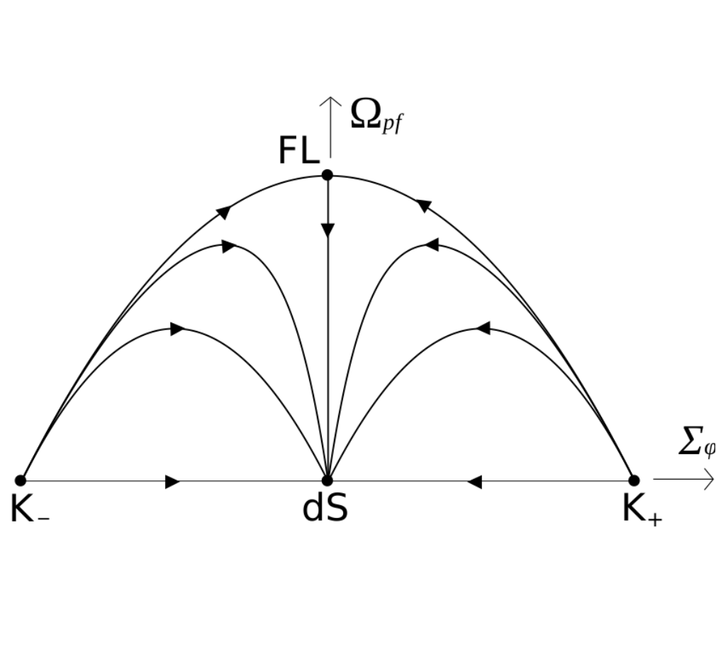
Recall that and for interior orbits. For a visual representation of the global orbit structure, see Figure 3(a).
Proof.
Using the methods in [16, 17] we derive the following monotonic function for region I:
| (24) |
which is strictly monotonically decreasing for all interior orbits since
| (25) |
where takes its minimum value, , at . Thus all interior orbits end at . Going backwards in time , which implies that . Taking the boundary structure into account together with the local fixed point analysis shows that one orbit originates from while all other interior orbits originate from the fixed points and .
The bifurcation value yields
| (26a) | ||||
| (26b) | ||||
| (26c) | ||||
As a consequence when . Furthermore, as follows from (26c), when interior orbits only go through an inflection point since (i.e., there is no invariant interior set with , ). Thus toward the future with the limit at , while and hence toward the past also in this case. Combining this with the boundary structure and the local analysis of the hyperbolic fixed points , and the center manifold analysis of yield the same result as when , which concludes the proof of Theorem 3.1. ∎
Theorem 3.2.
Global interior dynamics when .
- (i)
All interior orbits end at .
- (ii)
A single interior orbit originates from .
- (iii)
A 1-parameter set of interior orbits originate from .
- (iv)
When there is also a 1-parameter set of interior orbits that originates from , while a single interior orbit originates from .
- (v)
When all interior orbits apart from the single one from originate from .
Proof.
Using the methods developed in ch. 10 in [3] and [16, 17] result in the following monotonic function when is stable:
| (27) |
where is the value of at the fixed point , and where we note that when ; thus, the two exponents of and are thereby negative. The -fold time derivative of is given by
| (28) |
where when , but then and
| (29) |
where , and hence , except at the fixed point where and is a constant and hence all its derivatives are zero, exemplified by that with inserted yields zero. Thus just goes through an inflection point for the interior orbits when , . To summarize: is monotonically decreasing in the interior state space everywhere except at the fixed point . As a consequence decreases toward its positive minimum value at for all interior orbits, and thus they all end at . Furthermore, toward the past . Since both and this implies that or/and toward the past for all interior orbits. It follows from the orbits on the boundaries and , and the local fixed point analysis, that there is one orbit entering the state space from the fixed point and one from when . The remaining interior orbits originate from the fixed point only when and from both and when , each yielding 1-parameter set of orbits. ∎
This establishes the global solution structure for the present models for all and .99 9 For those that are so inclined, it is possible to formalize the above monotonicity arguments further with the Monotonicity Principle. The version on p. 103 in [3] is as follows: Let be a flow on with an invariant set. Let be a function whose range is the interval , where , and . If is decreasing on orbits in , then for all , the - and -limit sets of orbits in are given by and , respectively. A more advanced version of the monotonicity principle can be found in Appendix D in [29]. The solution structure is depicted in Figure 3.
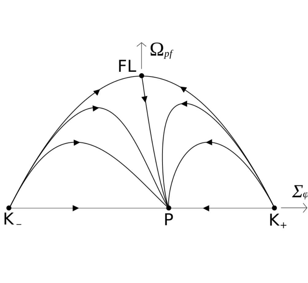
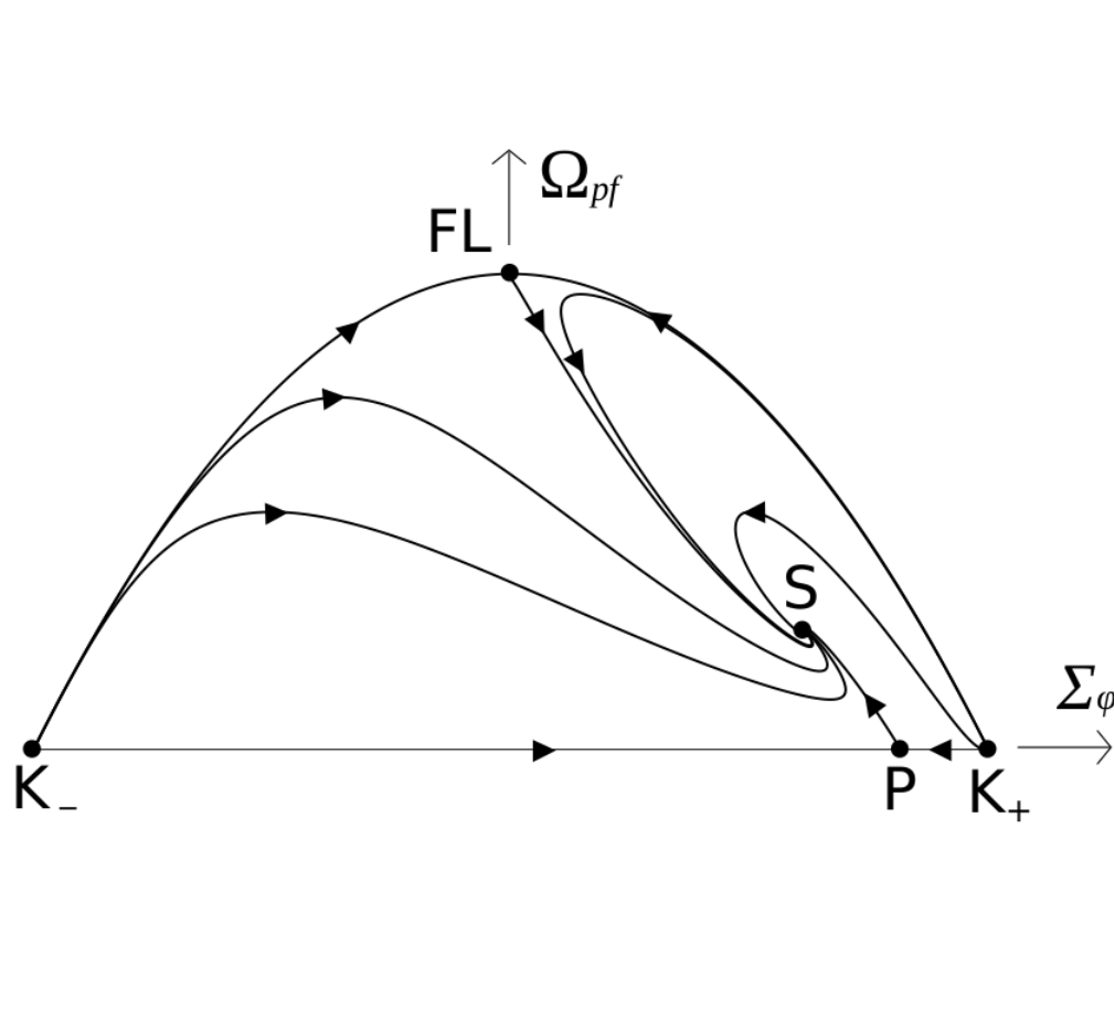
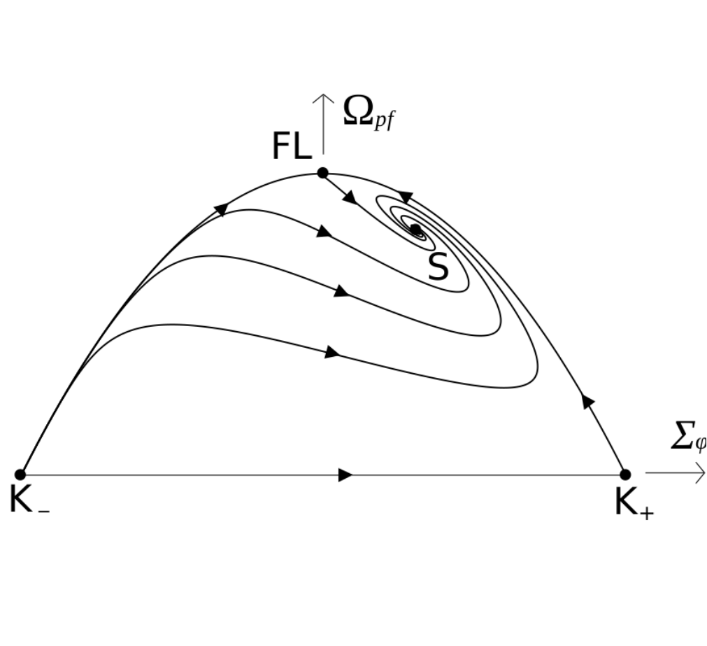
However, we here offer an alternative proof using a Dulac function instead of monotonic functions.
3.2 The Dulac function
In contrast to the previous direct proofs, the present one relies on the Poincaré-Bendixson theorem.
Theorem 3.3.
Global interior dynamics when .
-
The global dynamics of the dynamical system (11) can be inferred from the local stability analysis of the fixed points.
Proof.
The proof relies on the existence of a Dulac function and the simple boundary structure. Let , where and are the right hand sides of (11a) and (11b), respectively. In contrast to monotonic functions we do not have a systematic method for obtaining Dulac functions. However, since they are less restrictive for the dynamics it seems natural to make the ansatz . This gives
| (30) |
where . Choosing to eliminate the linear term and then to eliminate the and terms yield
| (31) |
i.e., the divergence of is strictly negative in the interior state space when . The function is thereby a Dulac function, which excludes the possibility of interior periodic orbits, see e.g. p. 265 in [28]. In combination with that there are no heteroclinic cycles on the boundary, it follows from the Poincaré-Bendixson theorem on (see e.g. [28] section 3.7) that the only possible - and -limit sets of the orbits (i.e., their future and past asymptotics) of the system (11) are the fixed points, i.e., the local analysis of the fixed points completely describes the future and past asymptotics of the dynamical system (11). ∎
In conclusion: In contrast to earlier work, we have performed a complete local and global analysis on FLRW models with a minimally coupled scalar field with an exponential potential and a perfect fluid with a linear equation of state. This has been accomplished by complementing previous linear analysis of hyperbolic fixed points with a center manifold analysis of non-hyperbolic fixed points, associated with bifurcations, and by constructing monotonic functions and a Dulac function that subsequently were used to give a global description of the dynamics of these models. The present analysis and methods serve as a starting point for investigations of models with more general asymptotically exponential potentials, and also for inhomogeneous perturbations of such models, topics that we will come back to in future papers.
Acknowledgments
It is a pleasure to thank John Wainwright for many useful discussions and for suggesting that we write the present paper. A. A. is supported by FCT/Portugal through CAMGSD, IST-ID, projects UIDB/04459/2020 and UIDP/04459/2020.
References
- [1] C. B. Collins. More qualitative cosmology. Comm. Math. Phys., 23(2):137–158, 1971.
- [2] O. I. Bogoyavlenskii and S. P. Novikov. Singularities of the cosmological model of the bianchi ix type according to the qualitative theory of differential equations. JETP, 37(5):747–755, 1973.
- [3] J. Wainwright and G. F. R. Ellis. Dynamical systems in cosmology. Cambridge University Press, 1997.
- [4] A. A. Coley. Dynamical systems and cosmology. Kluwer Academic Publishers, Dordrecht, 2003.
- [5] S. Bahamonde, C. G. Böhmer, S. Carloni, E. J. Copeland, W. F., and N. Tamanini. Dynamical systems applied to cosmology: Dark energy and modified gravity. Physics Reports, 775-777:1–122, 2018.
- [6] V. A. Belinskiǐ, L. P. Grishchuk, I. M. Khalatnikov, and Y. B. Zeldovich. Inflationary stages in cosmological models with a scalar field. Sov. Phys. JETP, 62:195, 1985.
- [7] V. A. Belinskiǐ, L. P. Grishchuk, I. M. Khalatnikov, and Y. B. Zeldovich. Inflationary stages in cosmological models with a scalar field. Phys. Lett., B155:232, 1985.
- [8] V. A. Belinskiǐ and I. M. Khalatnikov. On the generality of inflationary solutions in cosmological models with a scalar field. Sov. Phys. JETP, 66:441, 1987.
- [9] V. A. Belinskiǐ, H. Ishihara, I. M. Khalatnikov, and H. Sato. On the degree of generality of inflation in friedmann cosmological models with a massive scalar field. Prog. Theor. Phys., 79:676, 1988.
- [10] J. Halliwell. Scalar fields in cosmology with an exponential potential. Phys. Lett. B, 185:341, 1987.
- [11] B. Ratra and P. J. E. Peebles. Cosmological consequences of a rolling homogeneous scalar field. Phys. Rev. D, 37:3406, 1988.
- [12] A. A. Coley, J. Ibánez, and R. J. van den Hoogen. Homogeneous scalar field cosmologies with an exponential potential. Journal of Mathematical Physics, 38:17, 1997.
- [13] S. Foster. Scalar field cosmologies and the initial space-time singularity. Class. Quantum Grav., 15:3485, 1998.
- [14] E. J. Copeland, A. R. Liddle, and D. Wands. Exponential potentials and cosmological scaling solutions. Phys. Rev. D, 57:4686, 1998.
- [15] S. Foster. Scalar field cosmological models with hard potential walls. arXiv:gr-qc/9806113, 1998.
- [16] J. Heinzle and C Uggla. Monotonic functions in bianchi models: why they exist and how to find them. Class. Quantum Grav., 27:015009, 2010.
- [17] W. C. Hervik, S. Lim, P. Sandin, and C Uggla. Future asymptotics of tilted bianchi type ii cosmologies. Class. Quantum Grav., 27:185006, 2010.
- [18] A. Alho and C. Uggla. Scalar field deformations of lambda-cdm cosmology. Phys. Rev. D, 92(10):103502, 2015.
- [19] C. Uggla, R.T. Jantzen, and K. Rosquist. Exact hypersurface-homogeneous solutions in cosmology and astrophysics. Phys. Rev. D, 51:5522, 1995.
- [20] L. A. Urena-Lopez. Unified description of the dynamics of quintessential scalar fields. JCAP, 2012:035, 2012.
- [21] S. Tsujikawa. Quintessence: a review. Class. Quantum Grav., 30:214003, 2013.
- [22] H. Anzai. Ergodic skew product transformations on the torus. Osaka Math. J., 3:1, 1951.
- [23] A. Alho and C. Uggla. Global dynamics and inflationary center manifold and slow-roll approximants. Journal of Mathematical Physics, 56(012502), 2015.
- [24] A. Alho, J. Hell, and C. Uggla. Global dynamics and asymptotics for monomial scalar field potentials and perfect fluids. Class. Quant. Grav., 32(14):145005, 2015.
- [25] A. Alho and C. Uggla. Inflationary -attractor cosmology: A global dynamical systems perspective. Phys. Rev. D, 95(8):083517, 2017.
- [26] A. Alho, C. Uggla, and J. Wainwright. Quintessence. Preprint, 2021.
- [27] Michael Joyce and Tomislav Prokopec. Turning around the sphaleron bound: Electroweak baryogenesis in an alternative post-inflationary cosmology. Phys. Rev. D, 57:6022–6049, 1998.
- [28] L. Perko. Differential equation and dynamical systems, 3rd edition. Springer-Verlag, 2000.
- [29] M. Fjällborg, J. Heinzle, and C Uggla. Self-gravitating stationary spherically symmetric systems in relativistic galactic dynamics. Mathematical Proceedings of the Cambridge Philosophical Society, 143:731, 2007.