Efficient Sampling-Based Bayesian Active Learning for synaptic characterization

When using active learning in sequential experiments, three key elements need to be defined (Figure 1 (b)):

1. 1.

   The system to be studied: it is described by a generative model $\mathcal{M}$, which parameters $\theta$ can be inferred from its observed responses $y_{1:T}$ to a set of $T$ input stimuli $x_{1:T}$. Given the stochastic nature of most systems studied in biology, the random variable $Y_{1:T}$ corresponding to the observations can take various values $y_{1:T}$ according to a distribution $p(y_{1:T}|x_{1:T},\theta)$. In our application example of BAL, the system will be a model of binomial neurotransmitter release (see Section 2.2 The system: a binomial model of neurotransmitter release).

2. 2.

   A filter that computes the posterior distribution of the parameters given the previous inputs and observations $p(\theta|x_{1:t},y_{1:t})$: after each new input $x_{t+1}$ and observation $y_{t+1}$, it is updated to obtain $p(\theta|x_{1:t+1},y_{1:t+1})$ (see Section 2.3 The filter: online computation of the posterior distributions of parameters).

3. 3.

   A controller that computes the next optimal input stimuli $x_{t+1}^{*}$ so as to maximize a certain utility function, which is often defined as the mutual information between the parameter random variable $\Theta$ and the response random variable $Y_{t+1}$ given the experimental inputs $I_{x_{t+1}}(\Theta;Y_{t+1}|h_{t})$, where $h_{t}=(x_{1:t},y_{1:t})$ is the experiment history (see Section 2.4 The controller: computation of the optimal next stimulation time).

In synaptic characterization, inputs correspond to a set of $T$ stimulation times $x_{1:T}$ and observations correspond to recorded excitatory postsynaptic currents (EPSCs) $y_{1:T}$. In case of successive experiments (Park and Pillow 2012), the mutual information between the parameters and the next observation $Y_{t+1}$ conditioned on the experiment history $h_{t}$ is:

where $H(\Theta|h_{t})$ is the entropy of $\Theta$ given the experiment history up to time step $t$:

and

is the conditional entropy of $\Theta$ given the future observation random variable $Y_{t+1}$. Since the actual value of the future observation is unknown, we take the average over $y_{t+1}$ of the conditional entropy $H_{x_{t+1}}(\Theta|h_{,}Y_{t+1}=y_{t+1})$ conditioned on a certain value $y_{t+1}$. As the predictive distribution depends on the unknown parameters, we also have to take an average over $\theta$, using the current posterior distribution $p(\theta|h_{t})$ at time $t$ (Lewi et al. 2009):

The goal of Bayesian active learning is to select the next stimulation to maximize the mutual information between the parameters and all future observations:

where $\mathcal{S}_{t+1}$ is the set of possible inputs at time step $t+1$ and $\mathcal{S}_{t+2:t+n}$ is the set of possible protocols for the stimulations from time step $t+2$ to $t+n$. This set of protocols includes all the stimulation constraints, e.g. the remaining time of the experiment or the minimal inter-stimulation time. Optimizing all future inputs is an intractable problem (especially for online applications), since the algorithmic complexity scales exponentially with the number of observations $n$. For this reason, BAL only optimizes for the next stimulus (an approach referred to as a myopic design) (see Figure 1 (b)):

Different methods have been proposed to compute Eq. 6. Monte Carlo (MC) methods (Huan and Marzouk 2013) or a variational approach (Foster et al. 2019) can be employed, but they usually require long computation times that can be impractical if the time between successive experiments is short. Closed-form solutions can be computed only for some special cases, such as linear models or GLM (Lewi et al. 2009).

To illustrate our ESB-BAL framework, we apply it to the problem of estimating the parameters of a chemical synapse, represented as a state-space model with unobservable hidden states and input-dependent state transitions. A classical used model to describe the release of neurotransmitters at chemical synapses is called the binomial model (Katz 1969; Barri et al. 2016; Bird et al. 2016; Gontier and Pfister 2020; Stricker and Redman 2003; Scheuss and Neher 2001; Tsodyks et al. 1998). According to this model, a synapse is described as an Input-Output Hidden Markov Model (IO-HMM) with the following parameters (units are given in square brackets, see also Figure 1 (a)):

• •

  $N$ (the number of presynaptic independent release sites [-]);

• •

  $p$ (their release probability upon the arrival of a presynaptic spike [-]);

• •

  $\sigma$ (the standard deviation of the recording noise [A]);

• •

  $q$ (the quantum of current elicited in the postsynaptic cell by one release event [A]);

• •

  $\tau_{D}$ (the time constant of synaptic vesicle replenishment [s]).

The variables $n_{t}$ and $k_{t}$ represent, respectively, the number of available vesicles in the readily-releasable state at the moment of spike $t$ (with $0\leq n_{t}\leq N$), and the number of vesicles (among $n_{t}$) released after spike $t$ (with $0\leq k_{t}\leq n_{t}$). For simplicity, we use the notations $p_{\theta}(\cdot)=p(\cdot|\theta)$ with $\theta=[N,p,q,\sigma,\tau_{D}]$, and $z_{t}:=(n_{t},k_{t})$ to refer to the hidden variables at time step $t$.

The probability of recording a set of $T$ EPSCs $p_{\theta}(y_{1:T})$ is computed as the marginal of the joint distribution of the observations $y_{1:T}$ and the hidden variables $z_{1:T}$, i.e. $p_{\theta}(y_{1:T})=\sum_{z_{1:T}}p_{\theta}(y_{1:T},z_{1:T})$, where the joint distribution $p_{\theta}(y_{1:T},z_{1:T})=p_{\theta}(y_{1:T},n_{1:T},z_{1:T})$ is given by

where

is the emission probability, i.e. the probability to record output $y_{t}$ knowing that $k_{t}$ vesicles released neurotransmitter; $p_{\theta}(k_{t}|n_{t})$ is the binomial distribution and represents the probability that, given $n_{t}$ available vesicles, $k_{t}$ of them will indeed release neurotransmitter:

Finally, $p_{\theta}(n_{t}|n_{t-1},k_{t-1},x_{t})$ represents the process of vesicle replenishment. During the time interval $x_{t}$, each empty vesicle can refill with a probability $\pi(x_{t})=1-\exp\left(-\frac{x_{t}}{\tau_{D}}\right)$ such that the transition probability $p_{\theta}(n_{t}|n_{t-1},k_{t-1},x_{t})$ is given by:

One can note that $n_{t}=n_{t-1}-k_{t-1}+v_{t}$, where $v_{t}\sim\mathrm{Bin}({N-n_{t-1}+k_{t-1},\pi(x_{t})})$ is the number of refilled vesicles during the time interval $x_{t}$. Eqs. 7 to 10 define the observation model of the studied system (see Figure 1), i.e. the probability of a set of observations $y_{1:T}$ given a vector of stimuli $x_{1:T}$ and a vector of parameters $\theta$.

To be applicable for online experiments, the filtering block, which will compute the posterior distribution of parameters $p(\theta|h_{t})$, needs to satisfy two requirements:

1. 1.

   It must be sufficiently versatile to be applied to different systems and models;

2. 2.

   It must be online (i.e. its algorithmic complexity should not increase with the number of observations) (Bykowska et al. 2019).

A promising solution is particle filtering (Kutschireiter et al. 2020), and especially the Nested Particle Filter (NPF) (Crisan et al. 2018). This algorithm is asymptotically exact and purely recursive, thus allowing to directly estimate the parameters of a HMM as recordings are acquired.

The NPF relies on two nested layers of particles to approximate the posterior distributions of both the static parameters $\theta$ of the model and of its hidden states $z_{t}$. A first outer filter with $M_{\rm out}$ particles is used to compute the posterior distribution of parameters $p(\theta|h_{t})$, and for each of these particles, an inner filter with $M_{\rm in}$ particles is used to estimate the corresponding hidden states $z_{t}$ (so that the total number of particles in the system is $M_{\rm out}\times M_{\rm in}$). After each new observation, these particles are resampled based on their respective likelihoods, hence updating their posterior distributions (Figure 5).

The NPF was originally proposed for static HMMs, in which the state transition probability $p(z_{t+1}|z_{t},\theta)$ is supposed to be constant. Here, we extend it to the more general class of Input-Output Hidden Markov Models (IO-HMMs, also called GLM-HMMs in neuroscience, see Jha et al. 2022), in which the state transition probability at time step $t$ depends on an external input $x_{t}$. For instance, state transition in our model of synapse is not stationary, but depends on the ISI $x_{t}$ (see Section 3 Results).

The filter (Algorithm 1) relies on the following approximation to recursively compute the likelihood of each particle. Once the observation $y_{t}$ has been recorded, the likelihood of particle $\theta_{t}^{i}$, with $i\in\{1,...,M_{\rm out}\}$, depends on

with

If the variance of the jittering kernel $\kappa$ (which mutates the samples to avoid particles degeneracy and local solutions, see 5 Methods and Materials) is sufficiently small, and hence if $\theta_{t}^{i}\approx\theta_{t-1}^{i}$, the approximation $p(z_{t-1}|y_{1:t-1},\theta_{t}^{i})\approx p(z_{t-1}|y_{1:t-1},\theta_{t-1}^{i})$ allows to recursively compute Eq. 11. In practice, the different terms in Eq. 12 are computed as such: $p(y_{t}|z_{t},\theta_{t}^{i})$ corresponds to the Likelihood step of Algorithm 1; $p(z_{t}|z_{t-1},\theta_{t}^{i},x_{t})$ corresponds to the Propagation step; and $p(z_{t-1}|y_{1:t-1},\theta_{t}^{i})$ corresponds to the distribution of hidden states at time $t-1$.

Contrary to previous methods for fast posterior computation that were only applicable to specific models (Lewi et al. 2009), our filter can be applied to any state-space dynamical system, including non-stationary and input-dependent ones. Moreover, it does not require to approximate the posterior as a Gaussian nor require a time consuming (and possibly unstable) numerical optimization step, while being highly parallelizable and efficient (Besard et al. 2018; Besard et al. 2019).

The objective of experiment design optimization is to minimize the uncertainty of the estimates (classically quantified using the entropy) while reducing the cost of experimentation (defined as the number of required trials, samples, or observations). The optimal next stimulus $x_{t+1}^{*}$ that will maximize the mutual information (i.e. minimize the uncertainty about $\theta$ as measured by the entropy) can be written from Eqs. 1, 3, and 6 as

Eq. 13 requires to compute two (possibly high-dimensional) integrals over $\theta$ and $y_{t+1}$, for which closed-form expressions only exist for specific models. To avoid long MC simulations, we propose to use mean-field computations and to replace integrals by point-based approximations. Firstly, instead of computing the full expectation over $p(\theta|h_{t})$, we set $\theta$ to the mean posterior value $\hat{\theta}_{t}=\int d\theta p(\theta|h_{t})\theta$, which can be conveniently approximated as $\hat{\theta}_{t}\approx\frac{1}{M_{\rm out}}\sum_{i=1}^{M_{\rm out}}\theta_{t}^{i}$. Eq. 13 thus becomes

Depending on the nature of the studied system and on the time constraints of the experiment, different estimators can also be used, such as e.g. $\hat{\theta}_{t}=\argmax_{\theta}p(\theta|h_{t})$. Secondly, instead of computing the full expectation over the future observation, we set $y_{t+1}$ to its expected value; Eq. 13 thus becomes

In the general case, $\mathbb{E}(Y_{t+1}|h_{t},x_{t+1},\hat{\theta}_{t})$ can be computed using Bayesian Quadrature (Acerbi 2018). More specifically, for our model of a chemical synapse, an analytical formulation for the expected value $\mathbb{E}(Y_{t+1}|x_{1:t+1},\hat{\theta}_{t})$ can be efficiently derived using mean-field approximations (see Section 5.4 Mean-field approximation of vesicle dynamics). For each candidate $x_{t+1}$ in a given finite set $\mathcal{S}_{t+1}$, the entropy $H(\Theta|h_{t},x_{t+1},Y_{t+1}=\mathbb{E}(Y_{t+1}|h_{t},x_{t+1},\hat{\theta}_{t}))$ can be computed using Algorithm 1.

Finally, by assuming that the posterior distribution of $\Theta$ is well approximated by a Gaussian distribution (which is the case when there are sufficient observations (Paninski 2005)), its entropy can be estimated as $\frac{1}{2}\log|2\pi e\Sigma_{t}|$, where $\Sigma_{t}$ is the covariance matrix of the particles $\{\theta_{t}^{i}\}_{1\leq i\leq M_{\rm out}}$ (Jha et al. 2022).

From the experimentalist point of view, a highly relevant question is how to optimize the stimulation protocol such that the measured EPSCs are most informative about synaptic parameters. Previous studies showed that some stimulation protocols are more informative than others, but ignored the temporal correlations of the number of readily-releasable vesicles (Costa et al. 2013) or did not compute which protocol would be most informative (Barri et al. 2016). In classical deterministic experiment protocols, the stimulation times $x_{1:T}$ are defined and fixed prior to the recordings. By contrast, active learning optimises the protocol on the fly as data are recorded.

Results for a simulated experiment with ground-truth parameters $N^{*}=7$, $p^{*}=0.6$, $q^{*}=1$ pA, $\sigma^{*}=0.2$ pA, and $\tau_{D}^{*}=0.25$s (i.e. the same set of parameters $\theta^{*}$ used in Bird et al. 2016) are displayed in Figure 2 (a). Here, we compare ESB-BAL to three deterministic protocols:

• •

  in the Constant protocol, the synapse is probed at a constant frequency, i.e. $x_{t}=\rm cst$;

• •

  in the Uniform protocol, ISIs are uniformly drawn from a set $\mathcal{S}$ of candidates $x_{t}$ consisting of equidistantly separated values ranging from $x^{\rm min}=0.005$s (i.e. one order of magnitude shorter than the shortest ISI used in Barri et al. 2016) to $x^{\rm max}$, i.e. $x_{t}\sim\mathrm{Uniform}([0.005,x^{\rm max}])$;

• •

  finally, in the Exponential protocol, ISIs are drawn from an exponential distribution with mean $\tau$. Such a protocol has been shown to provide better estimates of synaptic parameters compared to periodic spike trains with constant ISI (Barri et al. 2016; Costa et al. 2013).

The efficiency of these deterministic protocols will depend on their respective parametrizations. To conservatively assess ESB-BAL, we optimize the values of $x_{t}$, $x^{\rm max}$, and $\tau$ so that the Constant, Uniform, and Exponential protocols have the best possible performance for the used ground-truth parameters $\theta^{*}$. Figure 6 shows the average final entropy decrease (i.e. the information gain) after 200 observations using the Constant (top), Uniform (middle), or Exponential (bottom) protocol, for different values of their hyperparameters. These deterministic protocols (with their optimal respective parametrizations) are then compared to ESB-BAL.

For the different protocols, the average (over 100 independent repetitions) joint differential entropy of the posterior distribution of parameters is plotted as a function of the number of observations (Figure 2 (a)). ESB-BAL allows to reduce the uncertainty (as measured by the entropy) of the parameter estimates for a given number of observations. It should be noted that it is compared to deterministic protocols whose respective hyperparameters have been optimized offline, knowing the value of $\theta^{*}$. In real physiology experiments, classical protocols are non-adaptative and are defined using (possibly sub-optimal) default parameters. In contrast, in active learning the protocol is optimized on the fly as data are recorded, and its performance will not depend on a prior parametrization. ESB-BAL thus outperforms the best possible Constant, Uniform, and Exponential protocols.

We also verify that ESB-BAL does not lead to biased estimates of $\theta$, as its average RMSE outperforms that of other protocols (Figure 2 (b)); and that it is sufficiently fast for online applications, as computation time exceeds the ISI in only a small proportion of cases (Figure 2 (c)). Similar results can be observed for different sets of ground-truth parameters $\theta^{*}$ (Figure 7) or when only optimizing for the entropy of a specific parameter (Figure 8).

Finally, in Figure 2 (a), ESB-BAL (black dashed line) is compared to exact active learning (gray dashed line), in which Eq. 13 is computed exactly using MC samples. Samples to compute the expectation over $\theta$ are drawn from $p(\theta|h_{t})$, whereas samples used to compute the expectation over $y_{t+1}$ are drawn from the generative distribution $p(y_{t+1}|h_{t},x_{t+1},\theta)$ (Eqs. 8, 9, and 10). This shows that the approximations used in Algorithm 2 to make active learning online have only a small effect on performance.

Active learning allows, for a given number of observations, to improve the reliability of the estimated parameters. However, in its classical implementation, only the next stimulus input is optimized, disregarding all future observations in the experiment. This myopic approach is thus sub-optimal. Moreover, neurophysiology experiments are not only constrained by the number of observations, but also by the total time of the experiment. Since cell viability and recording stability may become limiting during an experiment, the total time of an experimental protocol $\sum_{t=1}^{T}x_{t}$ also needs to be accounted for. Here, to account for the total time of the experiment, and to globally optimize the information gain per unit of time, we propose to modify the classical formulation of active learning (Eq. 13) by adding a penalty term for longer ISIs:

The effect of the penalty weight $\eta$ on the entropy of the posterior distribution of $\tau_{D}$ is displayed in Figure 3 (a). As expected, adding a penalty term to Eq. 13 reduces the precision of the inferred parameter. The loss of information gain increases with the penalty weight $\eta$. However, increasing $\eta$ also increases the speed of information gain, as seen in Figure 3 (b). Depending on the available time for the experiment, it is thus possible to tune $\eta$ so as to find a trade-off between long-term precision (Figure 3 (a)) and information rate (Figure 3 (b)).

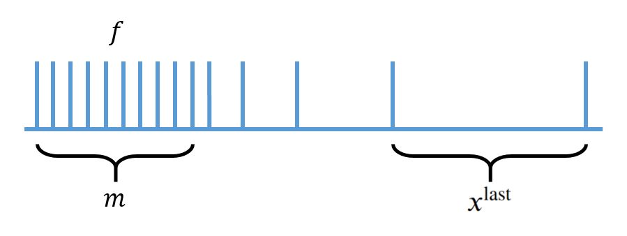
To reduce computational complexity, classical implementations of sequential experiment design usually only optimize for the immediate next observation. However, it might be critical for some systems to optimize not only the next stimulus, but rather the next $n$ stimuli of the experiment altogether (see Eq. 5) (Ryan et al. 2016; Drovandi et al. 2018). Synaptic characterization is a telling example: indeed, STD can only be observed for specifically organized batches of stimulation times. When probing the presynaptic cell, neuroscientists usually use repetitions of a spike train (Figure 4 (c)) consisting of a tetanic stimulation phase (sustained high-frequency stimulation used to deplete the presynaptic vesicles) followed by recovery spikes at increasing ISIs to probe the STD time constant (Markram et al. 1998). These spike trains (especially the duration and frequency of the tetanic phase, and the ISI between recovery spikes) are usually not optimized, and are held constant throughout an entire experiment.

Here, we show that ESB-BAL can be used to extend active learning to non-myopic designs, and to optimize the $n$ next input stimuli. Algorithm 3, which is a generalization of Algorithm 2, is used to select the next batch of $n$ stimuli $x_{t+1:t+n}^{*}$ in a set of candidate batches $\mathcal{S}_{t+1:t+n}$. Every $n$ observations, $H_{x_{t+1:t+n}}(\Theta|h_{t},Y_{t+1:t+n})$ is computed using $n$ iterations of the filter (i.e. Algorithm 1), in order to pick the optimal next batch $x_{t+1:t+n}^{*}$ that minimizes the quantity $H_{x_{t+1:t+n}}(\Theta|h_{t},Y_{t+1:t+n})$ (i.e. the posterior entropy over the parameters at time step $t+n$ given all observations up to time $t$):

We validate our method by applying it to EPSC recordings from acute mouse cerebellar slices (Figure 4 (a)): 5 mossy fiber to granule cell synaptic connections were studied. Each of them was stimulated using both ESB-BAL and different deterministic protocols: in deterministic protocols, the presynaptic cell is stimulated using a repetitive train stimulation consisting of either 20 or 100 stimuli at either 100 Hz or 300 Hz followed by 6 recovery pulses at increasing intervals.

For each stimulation protocol, the posterior distribution of the parameters was computed offline using the Metropolis-Hastings algorithm. Figure 4 (b1) shows the entropy at the end of the different stimulation protocols for the 5 studied synaptic connections. Each synapse was stimulated using several protocols (once with ESB-BAL, and at least once with a deterministic one), each having possibly different number of observations $T_{1},T_{2},T_{3}\dots$. Hence, for each synapse, only the first $T={\rm min}\{T_{1},T_{2},T_{3}\dots\}$ observations of each protocol were kept, to compare them for the same number of observations. In case a synapse was stimulated with several deterministic protocols, their respective entropies were averaged to only get one point in Figure 4 (b1). Panels (2) to (6) show the marginal posterior distributions for parameters of an example synapse, obtained using either ESB-BAL or a deterministic protocol (consisting of repetitions of the same train of 20 stimuli at 100Hz followed by 6 recovery spikes). Our results show that batch optimization via ESB-BAL significantly outperforms deterministic stimulation.

Candidate batches of stimulation times in $\mathcal{S}_{t+1:t+n}$ are parametrized with a low-dimensional parametrization to span different durations and frequencies for the tetanic phase, and different ISIs between the recovery spikes (see Figure 4 (c) and 5 Methods and Materials). They are chosen to span 3 parameters: the number $m<n$ of spikes in the tetanic stimulation phase, the frequency $f$ of spikes in the tetanic stimulation phase, and the duration of the final recovery ISI $x^{\rm last}$. The remaining $n-(m+1)$ spikes are then distributed geometrically between the end of the tetanic phase and the penultimate spike.

For a fixed model $\mathcal{M}$, the goal of BAL is to optimize the accuracy of the estimates of its parameters $\theta$, i.e. to minimize the entropy of the posterior distribution $p(\theta|x,y)$ (see Lindley 1956; Huan and Marzouk 2013 for a detailed discussion). The utility $\mathcal{U}(x,y)$ of a given experimental protocol $x$ and of a data set $y$ can be either defined as the gain in Shannon information between the prior and the posterior distribution of the parameters $\theta$, as suggested in Lindley 1956:

$\mathcal{U}(x,y)$ can also be defined as the Kullback-Leibler divergence between the prior and the posterior:

The expected utility $\mathcal{U}(x)$ of a protocol $x$ is finally the expected value of $\mathcal{U}(x,y)$ under $p(y|x)$, which yields the same result under (18) and (19):

It is worth noting that $\mathcal{U}(x)$ is actually the mutual information between $Y$ and $\Theta$. Indeed, Eq. (20) can be rewritten as

which yields $\mathcal{U}(x)=I_{x}(\Theta;Y)$. Different MCMC-based methods to compute $\mathcal{U}(x)$ are described in Huan and Marzouk 2013.

Initialisation: Computing the posterior distribution of $\theta$ firstly implies to specify a prior $p(\theta)$ from which the initial particles $\{\theta_{0}^{i}\}_{1\leq i\leq M_{\rm out}}$ will be drawn. For simplicity, we consider here uniform priors (as in Bird et al. 2016; Gontier and Pfister 2020), although the algorithm readily extends to different choices of prior.

Similarly, initial samples for the hidden states $\{n_{0}^{i,j},k_{0}^{i,j}\}_{1\leq j\leq M_{\rm in}}$ need to be drawn. For $i\in\{1,...,M_{\rm out}\}$, $j\in\{1,...,M_{\rm in}\}$, we define:

• •

  $n_{0}^{i,j}=N_{i}$ (i.e. all vesicles are supposed to be in the readily-releasable state at the beginning of the simulation);

• •

  $k_{0}^{i,j}\sim{\rm Bin}(N_{i},p_{i})$ (consistently with Eq. 9).

Jittering step: The parameters that we wish to infer are supposed to be constant. It is thus impossible to define dynamics of the form $p(\theta^{i}_{t+1}|\theta^{i}_{t})$ for the particles (as opposed to filtering problems aiming at inferring a dynamical hidden state, as for instance in Kutschireiter et al. 2017). To avoid particle degeneracy, it is thus necessary to mutate particles using a jittering kernel $\kappa(\theta_{t-1}^{i})$. When particles take continuous values, a classical choice for the jittering kernel is to draw the next particle $\theta_{t}^{i}$ from a Gaussian distribution with mean $\theta_{t-1}^{i}$ and which variance $\iota$ is called the jittering width (see Crisan et al. 2018 for a detailed discussion). In our implementation, the range of possible values for each parameter is discretized, so that each particle corresponds to a position on the grid of possible parameters values (same implementation as in Bird et al. 2016). The free parameter $\iota$ in our jittering kernel thus corresponds to the probability of moving by one bin:

where $\tilde{\theta}_{t-1}^{i}$ is one (randomly chosen) bin away from $\theta_{t-1}^{i}$.

Propagation step: Inner particles are redrawn based on $n_{t}^{i,j}\sim p(n_{t}^{i,j}|n_{t-1}^{i,j},k_{t-1}^{i,j},\theta_{t}^{i},x_{t})$ (Equation 10) and $k_{t}^{i,j}\sim p(k_{t}^{i,j}|n_{t}^{i,j},\theta_{t}^{i})$ (Equation 9).

Likelihood computation step: $p(y_{t}|n_{t}^{i,j},k_{t}^{i,j},\theta_{t}^{i})$ is computed according to Equation 8.

Resampling step: Particles are resampled using the algorithm introduced in Bentley and Saxe 1980, which allows to draw a list of sorted numbers in a single step.

Algorithm 2 is slightly modified in Figure 2 (a) for the ”ESB-BAL (exact)” simulations, in which Eq. 13 is computed using MC samples instead of the point-based simplifications explained in Eqs. 14 and 15. Samples to compute the expectation over $\theta$ are drawn from the current posterior distribution $p(\theta|h_{t})$, i.e. by random sampling from the pool of particles $\{\theta^{i}_{t}\}_{i\in\{1,\dots,M_{out}\}}$. For each of these samples, and for each candidate next input $x_{t+1}$ in $\mathcal{S}_{t+1}$, samples used to compute the expectation over $y_{t+1}$ are drawn by randomly sampling $n_{t+1}$, $k_{t+1}$, and $y_{t+1}$ (using respectively Eqs 10, 9, and 8) from the ground-truth values of the hidden states $n_{t}$ and $k_{t}$.

Our synapse model, as defined by Eq. 7 to 10, is a Hidden Markov Model with observations $y_{t}$ and hidden states $z_{t}=(n_{t},k_{t})$. The predictive distribution $p(y_{t+1}|h_{t},x_{t+1},\theta)$ used in Eq. 1 can be computed using the Baum-Welch algorithm: however, the algorithmic complexity of this forward-backward procedure, which scales with $N^{4}$, makes it impractical for closed-loop applications. Here, we suggest that computation can be massively simplified by using a mean-field approximation of vesicle dynamics: the analytical mean and variance of hidden and observed variables can be computed using recursive formulæ.

Let $r_{t}\in[0,1]$ denote the average fraction of release-competent vesicles at the moment of spike $t$. Its values, given $\theta=[N,p,q,\sigma,\tau_{D}]$ and $x_{1:t}$, can be iteratively computed (see Barri et al. 2016, Eq. (7)) from the equations of the Tsodyks-Markram model (Tsodyks et al. 1998):

with $r_{1}=1$. It follows that the expected value of the EPSC after spike $t$ is

One can note that the variance of the number of available vesicles $n_{t}$ conditioned on the history of previous activations $x_{1:t}$ and on the parameter values $\theta$ can be computed similarly using the law of total variance:

Since $n_{t}=n_{t-1}-k_{t-1}+v_{t}$ with $v_{t}\sim\mathrm{Bin}({N-n_{t-1}+k_{t-1},\pi(x_{t})})$ (see Eq. 10), it follows that

Finally, by noting that $(n_{t}-k_{t})|n_{t}\sim\mathrm{Bin}({n_{t},1-p})$ and using again the law of total variance to compute

we obtain

Each candidate batch of $n$ stimulation times in $\mathcal{S}_{t+1:t+n}$ (Figure 4 (b)) is described by 3 parameters:

• •

  $m<n$: the number of tetanic stimulations [-];

• •

  $f$: the frequency of the tetanic stimulations [Hz];

• •

  $x^{\rm last}$: the time interval before the final recovery spike [s].

A train of $n$ stimulations is thus composed of $m$ tetanic stimulations at a frequency $f$, followed by $n-m$ recovery spikes with increasing inter-spike intervals $\frac{x^{\rm last}}{n-m},\frac{x^{\rm last}}{n-m-1},\dots,\frac{x^{\rm last}}{2},x^{\rm last}$. The following values were used during experiments (Figure 4 (a)): $n=26$, $m\in[5,10,15,20]$, $f\in[25Hz,50Hz,100Hz,200Hz]$, $x^{\rm last}\in[0.1s,0.5s,1.0s,2.0s]$.

References

- Acerbi (2018) Acerbi L. Variational bayesian monte carlo. Advances in Neural Information Processing Systems. 2018; 31.
- Barri et al. (2016) Barri A, Wang Y, Hansel D, Mongillo G. Quantifying repetitive transmission at chemical synapses: a generative-model approach. Eneuro. 2016; 3(2).
- Bellman (1966) Bellman R. Dynamic programming. Science. 1966; 153(3731):34–37.
- Bentley and Saxe (1980) Bentley JL, Saxe JB. Generating sorted lists of random numbers. ACM Transactions on Mathematical Software (TOMS). 1980; 6(3):359–364.
- Besard et al. (2019) Besard T, Churavy V, Edelman A, De Sutter B. Rapid software prototyping for heterogeneous and distributed platforms. Advances in Engineering Software. 2019; 132:29–46.
- Besard et al. (2018) Besard T, Foket C, De Sutter B. Effective Extensible Programming: Unleashing Julia on GPUs. IEEE Transactions on Parallel and Distributed Systems. 2018; doi: 10.1109/TPDS.2018.2872064.
- Bhumbra and Beato (2013) Bhumbra GS, Beato M. Reliable evaluation of the quantal determinants of synaptic efficacy using Bayesian analysis. Journal of neurophysiology. 2013; 109(2):603–620.
- Bird et al. (2016) Bird AD, Wall MJ, Richardson MJ. Bayesian inference of synaptic quantal parameters from correlated vesicle release. Frontiers in computational neuroscience. 2016; 10:116.
- Bykowska et al. (2019) Bykowska O, Gontier C, Sax AL, Jia DW, Montero ML, Bird AD, Houghton C, Pfister JP, Costa RP. Model-based inference of synaptic transmission. Frontiers in synaptic neuroscience. 2019; 11:21.
- Carè et al. (2022) Carè M, Averna A, Barban F, Semprini M, De Michieli L, Nudo RJ, Guggenmos DJ, Chiappalone M. The impact of closed-loop intracortical stimulation on neural activity in brain-injured, anesthetized animals. Bioelectronic Medicine. 2022; 8(1):1–14.
- Costa et al. (2013) Costa RP, Sjostrom PJ, Van Rossum MC. Probabilistic inference of short-term synaptic plasticity in neocortical microcircuits. Frontiers in computational neuroscience. 2013; 7:75.
- Crisan et al. (2018) Crisan D, Miguez J, et al. Nested particle filters for online parameter estimation in discrete-time state-space Markov models. Bernoulli. 2018; 24(4A):3039–3086.
- Del Castillo and Katz (1954) Del Castillo J, Katz B. Quantal components of the end-plate potential. The Journal of physiology. 1954; 124(3):560–573.
- Drovandi et al. (2018) Drovandi CC, Tran MN, et al. Improving the efficiency of fully Bayesian optimal design of experiments using randomised quasi-Monte Carlo. Bayesian Analysis. 2018; 13(1):139–162.
- Emery and Nenarokomov (1998) Emery AF, Nenarokomov AV. Optimal experiment design. Measurement Science and Technology. 1998; 9(6):864.
- Flesch et al. (2018) Flesch T, Balaguer J, Dekker R, Nili H, Summerfield C. Comparing continual task learning in minds and machines. Proceedings of the National Academy of Sciences. 2018; 115(44):E10313–E10322.
- Foster et al. (2019) Foster A, Jankowiak M, Bingham E, Horsfall P, Teh YW, Rainforth T, Goodman N. Variational bayesian optimal experimental design. arXiv preprint arXiv:190305480. 2019; .
- Gontier (2022) Gontier C. Statistical approaches for synaptic characterization. PhD thesis, University of Bern; 2022.
- Gontier and Pfister (2020) Gontier C, Pfister JP. Identifiability of a Binomial Synapse. Frontiers in computational neuroscience. 2020; 14:86.
- Huan and Marzouk (2013) Huan X, Marzouk YM. Simulation-based optimal Bayesian experimental design for nonlinear systems. Journal of Computational Physics. 2013; 232(1):288–317.
- Jevons (1862) Jevons WS. The coal question. An Inquiry Concerning the Prog. 1862; .
- Jha et al. (2022) Jha A, Ashwood ZC, Pillow JW. Bayesian Active Learning for Discrete Latent Variable Models. arXiv preprint arXiv:220213426. 2022; .
- Kaeser and Regehr (2017) Kaeser PS, Regehr WG. The readily releasable pool of synaptic vesicles. Current opinion in neurobiology. 2017; 43:63–70.
- Katz (1969) Katz B. The release of neural transmitter substances. Liverpool University Press. 1969; p. 5–39.
- Kita et al. (2021) Kita K, Albergaria C, Machado AS, Carey MR, Müller M, Delvendahl I. GluA4 facilitates cerebellar expansion coding and enables associative memory formation. Elife. 2021; 10:e65152.
- Kutschireiter et al. (2020) Kutschireiter A, Surace SC, Pfister JP. The Hitchhiker’s guide to nonlinear filtering. Journal of Mathematical Psychology. 2020; 94:102307.
- Kutschireiter et al. (2017) Kutschireiter A, Surace SC, Sprekeler H, Pfister JP. Nonlinear Bayesian filtering and learning: a neuronal dynamics for perception. Scientific reports. 2017; 7(1):1–13.
- Lewi et al. (2009) Lewi J, Butera R, Paninski L. Sequential optimal design of neurophysiology experiments. Neural computation. 2009; 21(3):619–687.
- Lindley (1956) Lindley DV. On a measure of the information provided by an experiment. The Annals of Mathematical Statistics. 1956; p. 986–1005.
- Markram et al. (1998) Markram H, Pikus D, Gupta A, Tsodyks M. Potential for multiple mechanisms, phenomena and algorithms for synaptic plasticity at single synapses. Neuropharmacology. 1998; 37(4-5):489–500.
- Moreno-Bote et al. (2014) Moreno-Bote R, Beck J, Kanitscheider I, Pitkow X, Latham P, Pouget A. Information-limiting correlations. Nature neuroscience. 2014; 17(10):1410–1417.
- Paninski (2005) Paninski L. Asymptotic theory of information-theoretic experimental design. Neural Computation. 2005; 17(7):1480–1507.
- Park et al. (2011) Park M, Horwitz G, Pillow JW. Active learning of neural response functions with Gaussian processes. In: NIPS Citeseer; 2011. p. 2043–2051.
- Park and Pillow (2012) Park M, Pillow J. Bayesian active learning with localized priors for fast receptive field characterization. Advances in neural information processing systems. 2012; 25:2348–2356.
- Pfister et al. (2010) Pfister JP, Dayan P, Lengyel M. Synapses with short-term plasticity are optimal estimators of presynaptic membrane potentials. Nature neuroscience. 2010; 13(10):1271–1275.
- Ritzau-Jost et al. (2014) Ritzau-Jost A, Delvendahl I, Rings A, Byczkowicz N, Harada H, Shigemoto R, Hirrlinger J, Eilers J, Hallermann S. Ultrafast action potentials mediate kilohertz signaling at a central synapse. Neuron. 2014; 84(1):152–163.
- Ryan et al. (2016) Ryan EG, Drovandi CC, McGree JM, Pettitt AN. A review of modern computational algorithms for Bayesian optimal design. International Statistical Review. 2016; 84(1):128–154.
- Sargent et al. (2005) Sargent PB, Saviane C, Nielsen TA, DiGregorio DA, Silver RA. Rapid vesicular release, quantal variability, and spillover contribute to the precision and reliability of transmission at a glomerular synapse. Journal of Neuroscience. 2005; 25(36):8173–8187.
- Saviane and Silver (2006) Saviane C, Silver RA. Fast vesicle reloading and a large pool sustain high bandwidth transmission at a central synapse. Nature. 2006; 439(7079):983–987.
- Scheuss and Neher (2001) Scheuss V, Neher E. Estimating synaptic parameters from mean, variance, and covariance in trains of synaptic responses. Biophysical journal. 2001; 81(4):1970–1989.
- Sebastiani and Wynn (2000) Sebastiani P, Wynn HP. Maximum entropy sampling and optimal Bayesian experimental design. Journal of the Royal Statistical Society: Series B (Statistical Methodology). 2000; 62(1):145–157.
- Soares et al. (2019) Soares C, Trotter D, Longtin A, Béïque JC, Naud R. Parsing out the variability of transmission at central synapses using optical quantal analysis. Frontiers in synaptic neuroscience. 2019; 11:22.
- Stricker and Redman (2003) Stricker C, Redman SJ. Quantal analysis based on density estimation. Journal of neuroscience methods. 2003; 130(2):159–171.
- Sutton and Barto (2018) Sutton RS, Barto AG. Reinforcement learning: An introduction. MIT press; 2018.
- Tinkhauser and Moraud (2021) Tinkhauser G, Moraud EM. Controlling Clinical States Governed by Different Temporal Dynamics With Closed-Loop Deep Brain Stimulation: A Principled Framework. Frontiers in neuroscience. 2021; 15.
- Tsodyks et al. (1998) Tsodyks M, Pawelzik K, Markram H. Neural networks with dynamic synapses. Neural computation. 1998; 10(4):821–835.
- Wieland et al. (2021) Wieland FG, Hauber AL, Rosenblatt M, Tönsing C, Timmer J. On structural and practical identifiability. Current Opinion in Systems Biology. 2021; .
Appendix A Appendix