跳到论文正文
W Papers独立论文阅读器 arXiv:2201.07401 论文正文 计算阅读时间 · 0%
引用这篇论文根据当前论文元数据生成,正式投稿前建议核对。


License: CC BY-NC-SA 4.0
arXiv:2201.07401v2 [math.ST] 24 Jan 2023

Multiway Spherical Clustering via Degree-Corrected
Tensor Block ModelsThis paper was presented in part at 25th International Conference on Artificial Intelligence and Statistics (AISTATS).

Jiaxin Hu Affiliation: University of Wisconsin – Madison Email: jhu267@wisc.edu    Miaoyan Wang Affiliation: University of Wisconsin – Madison Email: miaoyan.wang@wisc.edu
Abstract

We consider the problem of multiway clustering in the presence of unknown degree heterogeneity. Such data problems arise commonly in applications such as recommendation system, neuroimaging, community detection, and hypergraph partitions in social networks. The allowance of degree heterogeneity provides great flexibility in clustering models, but the extra complexity poses significant challenges in both statistics and computation. Here, we develop a degree-corrected tensor block model with estimation accuracy guarantees. We present the phase transition of clustering performance based on the notion of angle separability, and we characterize three signal-to-noise regimes corresponding to different statistical-computational behaviors. In particular, we demonstrate that an intrinsic statistical-to-computational gap emerges only for tensors of order three or greater. Further, we develop an efficient polynomial-time algorithm that provably achieves exact clustering under mild signal conditions. The efficacy of our procedure is demonstrated through two data applications, one on human brain connectome project, and another on Peru Legislation network dataset.

Keywords: tensor clustering, degree correction, statistical-computational efficiency, human brain connectome networks

1 Introduction

Multiway arrays have been widely collected in various fields including social networks (Anandkumar et al., 2014), neuroscience (Wang et al., 2017), and computer science (Koniusz and Cherian, 2016). Tensors effectively represent the multiway data and serve as the foundation in higher-order data analysis. One data example is from multi-tissue multi-individual gene expression study (Wang et al., 2019; Hore et al., 2016), where the data tensor consists of expression measurements indexed by (gene, individual, tissue) triplets. Another example is hypergraph network (Ghoshdastidar and Dukkipati, 2017; Ghoshdastidar et al., 2017; Ahn et al., 2019; Ke et al., 2019) in social science. A KK-uniform hypergraph can be naturally represented as an order-KK tensor, where each entry indicates the presence of KK-way hyperedge among nodes (a.k.a. entities). In both examples, identifying the similarity among tensor entities is important for scientific discovery.

We study the problem of multiway clustering based on a data tensor. The goal of multiway clustering is to identify a checkerboard structure from a noisy data tensor. Figure 1 illustrates the noisy tensor and the underlying checkerboard structures discovered by multiway clustering methods. In the hypergraph example, the multiway clustering aims to identify the underlying block partition of nodes based on their higher-order connectivities; therefore, we also refer to the clustering as higher-order clustering. The most common model for higher-order clustering is called tensor block model (TBM) (Wang and Zeng, 2019), which extends the usual matrix stochastic block model (Abbe, 2018) to tensors. The matrix analysis tools, however, are sub-optimal for higher-order clustering. Developing tensor tools for solving block models has received increased interest recently (Wang and Zeng, 2019; Chi et al., 2020; Han et al., 2022a).

The classical tensor block model suffers from drawbacks to model real world data in spite of the popularity. The key underlying assumption of block model is that all nodes in the same community are exchangeable; i.e., the nodes have no individual-specific parameters apart from the community-specific parameters. However, the exchangeability assumption is often non-realistic. Each node may contribute to the data variation by its own multiplicative effect. We call the unequal node-specific effects the degree heterogeneity. Such degree heterogeneity appears commonly in social networks. Ignoring the degree heterogeneity may seriously mislead the clustering results. For example, the regular block model fails to model the member affiliation in the Karate Club network (Bickel and Chen, 2009) without addressing degree heterogeneity.

The degree-corrected tensor block model (dTBM) has been proposed recently to account for the degree heterogeneity (Ke et al., 2019). The dTBM combines a higher-order checkerboard structure with degree parameter 𝜽=(𝜽⁡(1),…,𝜽⁡(p))T\bm{\theta}=(\bm{\theta}(1),\ldots,\bm{\theta}(p))^{T} to allow heterogeneity among pp nodes. Figure 1 compares the underlying structures of TBM and dTBM with the same number of communities. The dTBM allows varying values within the same community, thereby allowing a richer structure. To solve dTBM, we project clustering objects to a unit sphere and perform iterative clustering based on angle similarity. We refer to the algorithm as the spherical clustering; detailed procedures are in Section 4. The spherical clustering avoids the estimation of nuisance degree heterogeneity. The usage of angle similarity brings new challenges to the theoretical results, and we develop new polar-coordinate based techniques in the proofs.

Refer to caption
Figure 1: Examples for order-3 tensor block model (TBM) with and without degree correction. Both TBM and dTBM have four communities on each mode, while dTBM allows a richer structure with degree heterogeneity.

Our contributions. The primary goal of this paper is to provide both statistical and computational guarantees for dTBM. Our main contributions are summarized below.

  • •

    We develop a general dTBM and establish the identifiability for the uniqueness of clustering using the notion of angle separability.

  • •

    We present the phase transition of clustering performance with respect to three different statistical and computational behaviors. We characterize, for the first time, the critical signal-to-noise (SNR) thresholds in dTBMs, revealing the intrinsic distinctions among (vector) one-dimensional clustering, (matrix) biclustering, and (tensor) higher-order clustering. Specific SNR thresholds and algorithm behaviors are depicted in Figure 2.

  • •

    We provide an angle-based algorithm that achieves exact clustering in polynomial time under mild conditions. Simulation and data studies demonstrate that our algorithm outperforms existing higher-order clustering algorithms.

The last two contributions, to our best knowledge, are new to the literature of dTBMs.

Figure 2: SNR thresholds for statistical and computational limits in order-KK dTBM with dimension (p,…,p)(p,...,p) and K≥2K\geq 2. The SNR gap between statistical possibility and computational efficiency exists only for tensors with K≥3K\geq 3.

Related work. Our work is closely related to but also distinct from several lines of existing research. Table 1 summarizes the most relevant models.

  • •

    Block model for clustering. The block model such as stochastic block model (SBM) and degree-corrected SBM has been widely used for matrix clustering problems. The theoretical properties and algorithm performance for matrix block models have been well-studied (Gao et al., 2018); see the review paper (Abbe, 2018) and the references therein. However, The tensor counterparts are relatively less understood.

  • •

    Tensor block model. The (non-degree) tensor block model (TBM) is a higher-order extension of SBM, and its statistical-computational properties are investigated in recent literatures (Wang and Zeng, 2019; Han et al., 2022a; Ghoshdastidar et al., 2017). Some works (Ahn et al., 2018) study the TBM with sparse observations, while, others (Wang and Zeng, 2019; Han et al., 2022a) and our work focus on the dense regime. Extending results from non-degree to degree-corrected model is highly challenging. Our dTBM parameter space is equipped with angle-based similarity and nuisance degree parameters. The extra complexity makes the Cartesian coordinates based analysis (Han et al., 2022a) non-applicable to our setting. Towards this goal, we have developed a new polar coordinates based analysis to control the model complexity. We have also developed a new angle-based iteration algorithm to achieve optimal clustering rates without the need of estimating nuisance degree parameters.

  • •

    Degree-corrected block model. The hypergraph degree-corrected block model (hDCBM) and its variant have been proposed in the literature (Ke et al., 2019; Yuan et al., 2022). For this popular model, however, the optimal statistical-computational rates remain an open problem. Our main contribution is to provide a sharp statistical and computational critical phase transition in dTBM literature. In addition, our algorithm results in a faster exponential error rate, in contrast to the polynomial rate in Ke et al., 2019. The original hDCBM (Ke et al., 2019) is designed for binary observations only, and we extend the model to both continuous and binary observations. We believe our results are novel and helpful to the community. See Figure 2 for overview of our results.

  • •

    Global-to-local algorithm strategy. Our methods generalize the recent global-to-local strategy for matrix learning (Gao et al., 2018; Chi et al., 2019; Yun and Proutiere, 2016) to tensors (Han et al., 2022a; Ahn et al., 2018; Kim et al., 2018). Despite the conceptual similarity, we address several fundamental challenges associated with this non-convex, non-continuous problem. We show the insufficiency of the conventional tensor HOSVD (De Lathauwer et al., 2000), and we develop a weighted higher-order initialization that relaxes the singular-value gap separation condition. Furthermore, our local iteration leverages the angle-based clustering in order to avoid explicit estimation of degree heterogeneity. Our bounds reveal the interesting interplay between the computational and statistical errors. We show that our final estimate provably achieves the exact clustering within only polynomial-time complexity.

Gao et al., 2018 Ahn et al., 2018 Han et al., 2022a Ghoshdastidar et al., 2017 Ke et al., 2019 Ours
Allow tensors of arbitrary order ×\times √\surd √\surd √\surd √\surd √\surd
Allow degree heterogeneity √\surd ×\times ×\times √\surd √\surd √\surd
Singular-value gap-free clustering √\surd √\surd √\surd ×\times ×\times √\surd
Misclustering rate (for order K∗K^{*}) - p−(K−1)​α−1∗⁣∗{p^{-(K-1)}\alpha^{-1}}^{**} exp⁡(−pK/2)\exp(-p^{K/2}) p−1p^{-1} p−2p^{-2} exp⁡(−pK/2)\exp(-p^{K/2})
Consider sparse observation ×\times √\surd ×\times ×\times ×\times ×\times
Table 1: Comparison between previous methods with our method. ∗We list the result for order-K tensors with K≥3K\geq 3 and general number of communities r=𝒪⁡(1)r=\mathcal{O}(1). ∗∗The parameter α=f⁡(p)>0\alpha=f(p)>0 denotes the sparsity level which is some function of dimension pp.

Notation. We use lower-case letters (e.g., a,ba,b) for scalars, lower-case boldface letters (e.g., 𝒂,𝜽\bm{a},\bm{\theta}) for vectors, upper-case boldface letters (e.g., 𝑿,𝒀\bm{X},\bm{Y}) for matrices, and calligraphy letters (e.g., 𝒳,𝒴\mathcal{X},\mathcal{Y}) for tensors of order three or greater. We use 𝟏p\mathbf{1}_{p} to denote a vector of length pp with all entries to be 1. We use |⋅||\cdot| for the cardinality of a set and 𝟙​{⋅}\mathds{1}\{\cdot\} for the indicator function. For an integer p∈ℕ+p\in\mathbb{N}_{+}, we use the shorthand [p]={1,2,…,p}[p]=\left\{1,2,...,p\right\}. For a length-pp vector 𝒂\bm{a}, we use a⁡(i)∈ℝa(i)\in\mathbb{R} to denote the ii-th entry of 𝒂\bm{a}, and use 𝒂I\bm{a}_{I} to denote the sub-vector by restricting the indices in the set I⊂[p]I\subset[p]. We use ‖𝒂‖=∑ia2​(i)\left\lVert\bm{a}\right\rVert=\sqrt{\sum_{i}a^{2}(i)} to denote the ℓ2\ell_{2}-norm, ‖𝒂‖1=∑i|ai|\left\lVert\bm{a}\right\rVert_{1}=\sum_{i}|a_{i}| to denote the ℓ1\ell_{1} norm of 𝒂\bm{a}. For two vector 𝒂,𝒃\bm{a},\bm{b} of the same dimension, we denote the angle between 𝒂,𝒃\bm{a},\bm{b} by

cos⁡(𝒂,𝒃)=⟨𝒂,𝒃⟩‖𝒂‖​‖𝒃‖,\cos\left(\bm{a},\bm{b}\right)=\frac{\left\langle\bm{a},\bm{b}\right\rangle}{\left\lVert\bm{a}\right\rVert\left\lVert\bm{b}\right\rVert}, (1)

where ⟨𝒂,𝒃⟩\left\langle\bm{a},\bm{b}\right\rangle is the inner product of two vectors and cos⁡(𝒂,𝒃)∈[−1,1]\cos\left(\bm{a},\bm{b}\right)\in[-1,1]. We make the convention that cos⁡(𝒂,𝒃)=cos⁡(𝒂T,𝒃T)\cos\left(\bm{a},\bm{b}\right)=\cos\left(\bm{a}^{T},\bm{b}^{T}\right).

Let 𝒴∈ℝp1×⋯×pK\mathcal{Y}\in\mathbb{R}^{p_{1}\times\cdots\times p_{K}} be an order-KK (p1,…,pK)(p_{1},...,p_{K})-dimensional tensor. We use 𝒴⁡(i1,…,iK)\mathcal{Y}(i_{1},\ldots,i_{K}) to denote the (i1,…,iK)(i_{1},\ldots,i_{K})-th entry of 𝒴\mathcal{Y}. The multilinear multiplication of a tensor 𝒮∈ℝr1×⋯×rK\mathcal{S}\in\mathbb{R}^{r_{1}\times\cdots\times r_{K}} by matrices 𝑴k∈ℝpk×rk\bm{M}_{k}\in\mathbb{R}^{p_{k}\times r_{k}} results in an order-KK (p1,…,pK)(p_{1},\ldots,p_{K})-dimensional tensor 𝒳\mathcal{X}, denoted

𝒳=𝒮×1𝑴1×⋯×K𝑴K,\mathcal{X}=\mathcal{S}\times_{1}\bm{M}_{1}\times\cdots\times_{K}\bm{M}_{K},

where the entries of 𝒳\mathcal{X} are defined by

𝒳(i1,…,iK)=∑(j1,…,jK)𝒮(j1,…,jK)𝑴1(i1,j1)⋯𝑴K(iK,jK).\displaystyle\mathcal{X}(i_{1},\ldots,i_{K})=\sum_{(j_{1},\ldots,j_{K})}\mathcal{S}(j_{1},\ldots,j_{K})\bm{M}_{1}(i_{1},j_{1})\cdots\bm{M}_{K}(i_{K},j_{K}). (2)

For a matrix 𝒀\bm{Y}, we use 𝒀i:\bm{Y}_{i:} (respectively, 𝒀:i\bm{Y}_{:i}) to denote the ii-th row (respectively, ii-th column) of the matrix. Similarly, for an order-3 tensor, we use 𝒴::i\mathcal{Y}_{::i} to denote the ii-th matrix slide of the tensor. We use Ave​(⋅)\text{Ave}(\cdot) to denote the operation of taking averages across elements and Matk​(⋅)\text{Mat}_{k}(\cdot) to denote the unfolding operation that reshapes the tensor along mode kk into a matrix. For a symmetric tensor 𝒳∈ℝp×⋯×p\mathcal{X}\in\mathbb{R}^{p\times\cdots\times p}, we omit the subscript and use Mat​(𝒳)∈ℝp×pK−1\text{Mat}(\mathcal{X})\in\mathbb{R}^{p\times p^{K-1}} to denote the unfolding. For two sequences {ap},{bp}\{a_{p}\},\{b_{p}\}, we denote ap≲bpa_{p}\lesssim b_{p} or ap=𝒪⁡(bp)a_{p}=\mathcal{O}(b_{p}) if limp→∞ap/bp≤c\lim_{p\to\infty}a_{p}/b_{p}\leq c, ap≳bpa_{p}\gtrsim b_{p} or ap=Ω⁡(bp)a_{p}=\Omega(b_{p}) if limp→∞ap/bp≥c\lim_{p\to\infty}a_{p}/b_{p}\geq c, for some constant c>0c>0, ap=o⁡(bp)a_{p}=o(b_{p}) if limp→∞ap/bp=0\lim_{p\to\infty}a_{p}/b_{p}=0, and ap≍bpa_{p}\asymp b_{p} if both bp≲apb_{p}\lesssim a_{p} and ap≲bpa_{p}\lesssim b_{p}. Throughout the paper, we use the terms “community” and “clusters” exchangeably.

Organization. The rest of this paper is organized as follows. Section 2 introduces the degree-corrected tensor block model (dTBM) with three motivating examples and presents the identifiability of dTBM under the angle gap condition. We show the phase transition and the existence of statistical-computational gaps for the higher-order dTBM in Section 3. In Section 4, we provide a polynomial-time two-stage algorithm with misclustering rate guarantees. Extension to Bernoulli models is also presented. In Section 5, we compare our work with non-degree tensor block models. Numerical studies including the simulation, comparison with other methods, and two real dataset analyses are in Sections 6-7. The main technical ideas we develop for addressing main theorems are provided in Section 8. Detailed proofs and extra theoretical results are provided in Appendix.

2 Model formulation and motivations

2.1 Degree-corrected tensor block model

Suppose that we have an order-KK data tensor 𝒴∈ℝp×⋯×p\mathcal{Y}\in\mathbb{R}^{p\times\cdots\times p}. Assume that there exist r≥1r\geq 1 disjoint communities among the pp nodes. We represent the community assignment by a function z:[p]↦[r]z\colon[p]\mapsto[r], where z⁡(i)=az(i)=a for ii-th node that belongs to the aa-th community. Then, z−1​(a)={i∈[p]:z⁡(i)=a}z^{-1}(a)=\{i\in[p]\colon z(i)=a\} denotes the set of nodes that belong to the aa-th community, and |z−1​(a)||z^{-1}(a)| denotes the number of nodes in the aa-th community. Let 𝜽=(θ⁡(1),…,θ⁡(p))T\bm{\theta}=(\theta(1),\ldots,\theta(p))^{T} denote the degree heterogeneity for pp nodes. We consider the order-KK dTBM (Ghoshdastidar et al., 2017; Ke et al., 2019),

𝒴⁡(i1,…,iK)=𝒮⁡(z⁡(i1),…,z⁡(iK))​∏k=1Kθik+ℰ⁡(i1,…,iK),\mathcal{Y}(i_{1},\ldots,i_{K})=\mathcal{S}(z(i_{1}),\ldots,z(i_{K}))\prod_{k=1}^{K}\theta_{i_{k}}+\mathcal{E}(i_{1},\ldots,i_{K}), (3)

where 𝒮∈ℝr×⋯×r\mathcal{S}\in\mathbb{R}^{r\times\cdots\times r} is an order-KK tensor collecting the block means among communities, and ℰ∈ℝp×⋯×p\mathcal{E}\in\mathbb{R}^{p\times\cdots\times p} is a noise tensor consisting of independent zero-mean sub-Gaussian entries with variance bounded by σ2\sigma^{2}. The unknown parameters are zz, SS, and 𝜽\bm{\theta}. The dTBM can be equivalently written in a compact form of tensor-matrix product:

𝔼𝒴=𝒮×1𝚯𝑴×2⋯×K𝚯𝑴,\mathbb{E}\mathcal{Y}=\mathcal{S}\times_{1}\bm{\Theta}\bm{M}\times_{2}\cdots\times_{K}\bm{\Theta}\bm{M}, (4)

where 𝚯=diag​(θ⁡(1),…,θ⁡(p))∈ℝp×p\bm{\Theta}=\text{diag}(\theta(1),...,\theta(p))\in\mathbb{R}^{p\times p} is a diagonal matrix, 𝑴∈{0,1}p×r\bm{M}\in\left\{0,1\right\}^{p\times r} is the membership matrix associated with community assignment zz such that 𝑴(i,j)=𝟙{z(i)=j}\bm{M}(i,j)=\mathds{1}\{z(i)=j\}. By definition, each row of 𝑴\bm{M} has one copy of 1’s and 0’s elsewhere. Note that the discrete nature of 𝑴\bm{M} renders our model (4) more challenging than Tucker decomposition. We call a tensor 𝒴\mathcal{Y} an rr-block tensor with degree 𝜽\bm{\theta} if 𝒴\mathcal{Y} admits dTBM (4) and let 𝒳=𝔼​𝒴\mathcal{X}=\mathbb{E}\mathcal{Y} denote the mean tensor. The goal of clustering is to estimate zz from a single noisy tensor 𝒴\mathcal{Y}. We are particularly interested in the high-dimensional regime where pp grows whereas r=𝒪⁡(1)r=\mathcal{O}(1).

For ease of notation, we have focused on the case with symmetric mean tensor 𝔼​𝒴\mathbb{E}\mathcal{Y}. This assumption simplifies the notation because all modes have the same (𝚯,𝑴,z)(\bm{\Theta},\bm{M},z); the noise tensor ℰ\mathcal{E} and the data tensor 𝒴\mathcal{Y} are still possibly asymmetric. In general, we allow asymmetric mean tensors with {(𝚯k,𝑴k,zk)}k=1K\{(\bm{\Theta}_{k},\bm{M}_{k},z_{k})\}_{k=1}^{K}, one for each mode. The extension can be found in Appendix B.

2.2 Motivating examples

Here, we provide four applications to illustrate the practical necessity of dTBM.

Tensor block model

Consider the model (4). Let θ⁡(i)=1\theta(i)=1 for all i∈[p]i\in[p]. The model (4) reduces to the tensor block model, which is widely used in previous clustering algorithms (Wang and Zeng, 2019; Chi et al., 2020; Han et al., 2022a). The theoretical results in TBM serve as benchmarks for dTBM.

Community detection in hypergraphs

The hypergraph network is a powerful tool to represent the complex entity relations with higher-order interactions (Ke et al., 2019). A typical undirected hypergraph is denoted as H=(V,E)H=(V,E), where V=[p]V=[p] is the set of nodes and EE is the set of undirected hyperedges. Each hyperedge in EE is a subset of VV, and we call the hyperedge an order-KK edge if the corresponding subset involves KK nodes. We call HH a KK-uniform hypergraph if EE only contains order-KK edges.

It is natural to represent the KK-uniform hypergraph using a binary order-KK adjacency tensor. Let 𝒴∈{0,1}p×⋯×p\mathcal{Y}\in\{0,1\}^{p\times\cdots\times p} denote the adjacency tensor, where the entries encode the presence or absence of order-KK edges among pp nodes. Specifically, for all (i1,…,iK)∈[p]K(i_{1},\ldots,i_{K})\in[p]^{K}, we have

𝒴⁡(i1,…,iK)={1if ​(i1,…,iK)∈E,0if ​(i1,…,iK)∉E.\mathcal{Y}(i_{1},...,i_{K})=\begin{cases}1&\text{if }(i_{1},...,i_{K})\in E,\\ 0&\text{if }(i_{1},...,i_{K})\notin E.\end{cases} (5)

Assume that there exist rr disjoint communities among pp nodes, and the connection probabilities depend on the community assignments and node-specific parameters. Then, the equation (4) models 𝔼​𝒴\mathbb{E}\mathcal{Y} with unknown degree heterogeneity 𝜽\bm{\theta} and sub-Gaussianity parameter σ2=1/4\sigma^{2}=1/4.

Multi-layer weighted network

Multi-layer weighted network data consists of multiple networks over the same set of nodes. One representative example is the brain connectome data (Zhang et al., 2019). The multi-layer weighted network 𝒴\mathcal{Y} has dimension of p×p×Lp\times p\times L, where pp denotes the number of brain regions of interest, and LL denotes the number of layers (networks). Each of the LL networks describes one aspect of the brain connectivity, such as functional connectivity or structural connectivity. The resulting tensor 𝒴\mathcal{Y} consists of a mixture of slices with various data types.

Assume that there exist rr disjoint communities among pp nodes and rlr_{l} disjoint communities among the LL layers. The multi-layer network community detection is modeled by the general asymmetric dTBM model (4)

𝔼𝒴=𝒮×1𝚯𝑴×2𝚯𝑴×3𝚯l𝑴l,\mathbb{E}\mathcal{Y}=\mathcal{S}\times_{1}\bm{\Theta}\bm{M}\times_{2}\bm{\Theta}\bm{M}\times_{3}\bm{\Theta}_{l}\bm{M}_{l}, (6)

where (𝜽∈ℝp,𝑴∈{0,1}p×r)(\bm{\theta}\in\mathbb{R}^{p},\bm{M}\in\{0,1\}^{p\times r}) and (𝜽l∈ℝL,𝑴l∈{0,1}L×rl)(\bm{\theta}_{l}\in\mathbb{R}^{L},\bm{M}_{l}\in\{0,1\}^{L\times r_{l}}) are the degree heterogeneity and membership matrices corresponding to the community structure for pp nodes and LL layers, respectively.

Gaussian higher-order clustering

Datasets in various fields such as medical image, genetics, and computer science are formulated as Gaussian tensors. One typical example is the multi-tissue gene expression dataset, which records different gene expressions in different individuals and different tissues. The dataset, denoted as 𝒴∈ℝp×n×t\mathcal{Y}\in\mathbb{R}^{p\times n\times t}, consists of the expression data for pp genes of nn individuals in tt tissues.

Assume that there exist r1,r2,r3r_{1},r_{2},r_{3} disjoint clusters for pp genes, nn individuals, and tt tissues, respectively. We apply the general asymmetric dTBM model (4)

𝔼𝒴=𝒮×1𝚯1𝑴1×2𝚯2𝑴2×3𝚯3𝑴3,\mathbb{E}\mathcal{Y}=\mathcal{S}\times_{1}\bm{\Theta}_{1}\bm{M}_{1}\times_{2}\bm{\Theta}_{2}\bm{M}_{2}\times_{3}\bm{\Theta}_{3}\bm{M}_{3}, (7)

where {(𝜽k,𝑴k)}k=13\{(\bm{\theta}_{k},\bm{M}_{k})\}_{k=1}^{3} represents the degree heterogeneity and membership for genes, individuals, and tissues.

Remark 1 (Comparison with non-degree models).

Our dTBM uses fewer block parameters than TBM. In particular, every non-degree r1r_{1}-block tensor can be represented by a degree-corrected r2r_{2}-block tensor with r2≤r1r_{2}\leq r_{1}. In particular, there exist tensors with r1=pr_{1}=p but r2=1r_{2}=1, so the reduction in model complexity can be dramatic from pp to 1. This fact highlights the benefits of introducing degree heterogeneity in higher-order clustering tasks.

2.3 Identifiability under angle gap condition

The goal of clustering is to estimate the partition function zz from model (4). For ease of notation, we focus on symmetric tensors; the extension to non-symmetric tensors are similar. We use 𝒫\mathcal{P} to denote the following parameter space for (z,𝒮,𝜽)(z,\mathcal{S},\bm{\theta}),

𝒫=\displaystyle\mathcal{P}= {(z,𝒮,𝜽):𝜽∈ℝ+p,c1​pr≤|z−1(a)|≤c2​pr,c3≤∥Mat(𝒮)a:∥≤c4,‖𝜽z−1​(a)‖1=|z−1(a)|,a∈[r]}\displaystyle\bigg\{(z,\mathcal{S},\bm{\theta})\colon\ \bm{\theta}\in\mathbb{R}^{p}_{+},\ {c_{1}p\over r}\leq|z^{-1}(a)|\leq{c_{2}p\over r},c_{3}\leq\lVert\text{Mat}(\mathcal{S})_{a:}\rVert\leq c_{4},\left\lVert\bm{\theta}_{z^{-1}(a)}\right\rVert_{1}=|z^{-1}(a)|,a\in[r]\bigg\} (8)

where ci>0c_{i}>0’s are universal constants. We briefly describe the rationale of the constraints in (8). First, the entrywise positivity constraint on 𝜽∈ℝ+p\bm{\theta}\in\mathbb{R}^{p}_{+} is imposed to avoid sign ambiguity between entries in 𝜽z−1​(a)\bm{\theta}_{z^{-1}(a)} and 𝒮\mathcal{S}. This constraint allows the trigonometric cos\cos to describe the angle similarity in the Assumption 1 below and Sub-algorithm 2 in Section 4. Note that the positivity constraint can be achieved without sacrificing model flexibility, by using a slightly larger dimension of 𝒮\mathcal{S} in the factorization (4); see Example 1 below. Second, recall that the quantity |z−1​(a)||z^{-1}(a)| denotes the number of nodes in the aa-th community. The constants c1,c2c_{1},c_{2} in the |z−1​(a)||z^{-1}(a)| bounds assume the roughly balanced size across rr communities. Third, the constant c3c_{3} requires that all slides in 𝒮\mathcal{S} have non-degenerate norm. Particularly, the lower bound c3c_{3} excludes the purely zero slide to avoid trivial non-identifiability of model (4); see Example 2 below. The upper bound c4c_{4} is a technical constraint to avoid the slides with diverging norm as dimension grows. Lastly, the ℓ1\ell_{1} normalization ∥𝜽z−1​(a)∥1=|z−1​(a)|\lVert\bm{\theta}_{z^{-1}(a)}\rVert_{1}=|z^{-1}(a)| is imposed to avoid the scalar ambiguity between 𝜽z−1​(a)\bm{\theta}_{z^{-1}(a)} and 𝒮\mathcal{S}. This constraint, again, incurs no restriction to model flexibility but makes our presentation cleaner. Our constraints in 𝒫\mathcal{P} are mild compared with previous literature; see Table 2 for comparison.

Example 1 (Positivity of degree parameters).

Here we provide an example to show the positivity constraint on 𝜽\bm{\theta} incurs no loss on the model flexibility. Consider an order-3 dTBM with core tensor 𝒮=1\mathcal{S}=1 and degree 𝜽=(1,1,−1,−1)T\bm{\theta}=(1,1,-1,-1)^{T}. We have the mean tensor

𝒳=𝒮×1𝚯𝑴×2𝚯𝑴×3𝚯𝑴,\mathcal{X}=\mathcal{S}\times_{1}\bm{\Theta}\bm{M}\times_{2}\bm{\Theta}\bm{M}\times_{3}\bm{\Theta}\bm{M}, (9)

where 𝚯=diag​(𝜽)\bm{\Theta}=\text{diag}(\bm{\theta}) and 𝑴=(1,1,1,1)T\bm{M}=(1,1,1,1)^{T}. Note that 𝒳∈ℝ4×4×4\mathcal{X}\in\mathbb{R}^{4\times 4\times 4} is a 1-block tensor with mixed-signed degree 𝜽\bm{\theta}, and the mode-3 slices of 𝒳\mathcal{X} are

𝒳::1=𝒳::2=−𝒳::3=−𝒳::4=[11−1−111−1−1−1−111−1−111].\mathcal{X}_{::1}=\mathcal{X}_{::2}=-\mathcal{X}_{::3}=-\mathcal{X}_{::4}=\begin{bmatrix}1&1&-1&-1\\ 1&1&-1&-1\\ -1&-1&1&1\\ -1&-1&1&1\end{bmatrix}. (10)

Now, instead of original decomposition, we encode 𝒳\mathcal{X} as a 2-block tensor with positive-signed degree. Specifically, we write

𝒳=𝒮′×1𝚯′𝑴′×2𝚯′𝑴′×3𝚯′𝑴′,\mathcal{X}=\mathcal{S}^{\prime}\times_{1}\bm{\Theta}^{\prime}\bm{M}^{\prime}\times_{2}\bm{\Theta}^{\prime}\bm{M}^{\prime}\times_{3}\bm{\Theta}^{\prime}\bm{M}^{\prime}, (11)

where 𝚯′=diag​(𝜽′)=diag​(1,1,1,1)\bm{\Theta}^{\prime}=\text{diag}(\bm{\theta}^{\prime})=\text{diag}(1,1,1,1), the core tensor 𝒮′∈ℝ2×2×2\mathcal{S}^{\prime}\in\mathbb{R}^{2\times 2\times 2} has following mode-3 slices, and the membership matrix 𝑴′∈{0,1}4×2\bm{M}^{\prime}\in\{0,1\}^{4\times 2} defines the clustering z′:[4]→[2]z^{\prime}\colon[4]\to[2]; i.e.,

𝒮′::1=−𝒮′::2=[1−1−11],𝑴′=[10100101].\mathcal{S}^{\prime}_{::1}=-\mathcal{S}^{\prime}_{::2}=\begin{bmatrix}1&-1\\ -1&1\end{bmatrix},\quad\bm{M}^{\prime}=\begin{bmatrix}1&0\\ 1&0\\ 0&1\\ 0&1\end{bmatrix}. (12)

The triplet (z′,𝒮′,𝜽′)(z^{\prime},\mathcal{S}^{\prime},\bm{\theta}^{\prime}) lies in our parameter space (8). In general, we can always reparameterize an rr-block tensor with mixed-signed degree using a 2​r2r-block tensor with positive-signed degree. Since we assume r=𝒪⁡(1)r=\mathcal{O}(1) throughout the paper, the splitting does not affect the error rates of our interest.

Example 2 (Non-identifiability with purely zero core slice).

Consider an order-2 dTBM with core tensor 𝑺=(001−1)\bm{S}=\begin{pmatrix}0&0\\ 1&-1\end{pmatrix} degree matrices 𝚯1=𝚯2=diag​(1,1,1,1)\bm{\Theta}_{1}=\bm{\Theta}_{2}=\text{diag}(1,1,1,1), and mean tensor

𝒳=𝚯1​𝑴​𝑺​𝑴T​𝚯2,with ​𝑴=[10100101].\mathcal{X}=\bm{\Theta}_{1}\bm{M}\bm{S}\bm{M}^{T}\bm{\Theta}_{2},\quad\text{with }\bm{M}=\begin{bmatrix}1&0\\ 1&0\\ 0&1\\ 0&1\\ \end{bmatrix}. (13)

Replacing 𝚯1\bm{\Theta}_{1} by 𝚯1′=(3/2,1/2,1,1)\bm{\Theta}^{\prime}_{1}=(3/2,1/2,1,1) leads to the same mean tensor 𝒳\mathcal{X}.

Assumptions in parameter space Gao et al., 2018 Han et al., 2022a Ke et al., 2019 Ours
Balanced community sizes √\surd √\surd √\surd √\surd
Bounded core tensors √\surd ×\times √\surd √\surd
Balanced degrees √\surd - √\surd √\surd
Flexible in-group connections ×\times √\surd √\surd √\surd
Gaps among cluster centers In-between cluster difference Euclidean gap Eigen gap Angle gap
Table 2: Parameter space comparison between previous work with our assumption.

We now provide the identifiability conditions for our model before estimation procedures. When r=1r=1, the decomposition (4) is always unique (up to cluster label permutation) in 𝒫\mathcal{P}, because dTBM is equivalent to the rank-1 tensor family under this case. When r≥2r\geq 2, the Tucker rank of signal tensor 𝔼​𝒴\mathbb{E}\mathcal{Y} in (4) is bounded by, but not necessarily equal to, the number of blocks rr (Wang and Zeng, 2019). Therefore, one can not apply the classical identifiability conditions for low-rank tensors to dTBM. Here, we introduce a key separation condition on the core tensor.

Assumption 1 (Angle gap).

Let 𝑺=Mat​(𝒮)\bm{S}=\text{Mat}(\mathcal{S}). Assume that the minimal gap between normalized rows of 𝑺\bm{S} is bounded away from zero; i.e.,

Δmin:=mina≠b∈[r]‖𝑺a:∥𝑺a:∥−𝑺b:∥𝑺b:∥‖>0,forr≥2.\Delta_{\min}:=\min_{a\neq b\in[r]}\left\lVert\frac{\bm{S}_{a:}}{\lVert\bm{S}_{a:}\rVert}-\frac{\bm{S}_{b:}}{\lVert\bm{S}_{b:}\rVert}\right\rVert>0,\quad\text{for}\quad r\geq 2. (14)

We make the convention Δmin=1\Delta_{\min}=1 for r=1r=1. Equivalently, (14) says that none of the two rows in 𝑺\bm{S} are parallel; i.e., maxa≠b∈[r]cos(𝑺a:,𝑺b:)=1−Δmin2/2<1\max_{a\neq b\in[r]}\cos\left(\bm{S}_{a:},\ \bm{S}_{b:}\right)=1-\Delta^{2}_{\min}/2<1. The quantity Δmin\Delta_{\min} characterizes the non-redundancy among clusters measured by angle separation. The denominators involved in definition (14) are well posed because of the lower bound on ‖𝑺a:‖\left\lVert\bm{S}_{a:}\right\rVert in (8).

Our first main result is the following theorem showing the sufficiency and necessity of the angle gap separation condition for the parameter identifiability under dTBM.

Theorem 1 (Model identifiability).

Consider the dTBM with r≥2r\geq 2 and K≥2K\geq 2. The parameterization (4) is unique in 𝒫\mathcal{P} up to cluster label permutations, if and only if Assumption 1 holds.

The identifiability guarantee for the dTBM is stronger than classical Tucker model. In the Tucker model, the factor matrix 𝑴\bm{M} is identifiable only up to orthogonal rotations. In contrast, our model does not suffer from rotational invariance. As we will show in Section 4, each column of the membership matrix 𝑴\bm{M} can be precisely recovered under our algorithm. This property benefits the interpretation of dTBM in practice.

3 Statistical-computational critical values for higher-order tensors

3.1 Assumptions

We propose the signal-to-noise ratio (SNR),

SNR:=Δmin2/σ2=pγ,\displaystyle\text{SNR}:=\Delta^{2}_{\min}/\sigma^{2}=p^{\gamma}, (15)

with varying γ∈ℝ\gamma\in\mathbb{R} that quantifies different regimes of interest. We call γ\gamma the signal exponent. Intuitively, a larger SNR, or equivalently a larger γ\gamma, benefits the clustering in the presence of noise. With quantification (15), we consider the following parameter space,

𝒫⁡(γ)=𝒫∩{𝒮​ satisfies SNR condition (15) with γ}.\mathcal{P}(\gamma)=\mathcal{P}\cap\{\mathcal{S}\text{ satisfies SNR condition~\eqref{eq:gamma} with $\gamma$}\}. (16)

The 11-block dTBM does not belong to the space 𝒫⁡(γ)\mathcal{P}(\gamma) when γ<0\gamma<0, due to the convention in Assumption 1. Our goal is to characterize the clustering accuracy with respect to γ\gamma under the space 𝒫⁡(γ)\mathcal{P}(\gamma).

In our algorithmic development, we often refer to the regime of balanced degree heterogeneity. We call the degree 𝜽\bm{\theta} balanced if

mina∈[r]⁡∥𝜽z−1​(a)∥=(1+o⁡(1))​maxa∈[r]​∥𝜽z−1​(a)∥.{\min_{a\in[r]}\lVert\bm{\theta}_{z^{-1}(a)}\rVert=\left(1+o(1)\right)\max_{a\in[r]}\lVert\bm{\theta}_{z^{-1}(a)}\rVert}. (17)

The following lemma provides the rationale of balanced degree assumption. We show the close relation between angle gaps in the mean tensor 𝒳\mathcal{X} and the core tensor 𝒮\mathcal{S} under balanced degree heterogeneity.

Lemma 1 (Angle gaps in 𝒳\mathcal{X} and 𝒮\mathcal{S}).

Consider the dTBM model (4) under the parameter space 𝒫\mathcal{P} in (8) with r≥2r\geq 2. Suppose 𝜽\bm{\theta} is balanced satisfying (17) and mini∈[p]⁡θ⁡(i)≥c\min_{i\in[p]}\theta(i)\geq c from some constant c>0c>0. Then, as p→∞p\rightarrow\infty, for all i,ji,j such that z⁡(i)≠z⁡(j)z(i)\neq z(j), we have

cos(𝑿i:,𝑿j:)≍cos(𝑺z⁡(i):,𝑺z⁡(j):),\cos(\bm{X}_{i:},\bm{X}_{j:})\asymp\cos(\bm{S}_{z(i):},\bm{S}_{z(j):}), (18)

where 𝑿=Mat​(𝒳)\bm{X}=\text{Mat}(\mathcal{X}) and 𝑺=Mat​(𝒮)\bm{S}=\text{Mat}(\mathcal{S}).

In practice, an estimation algorithm has access to a noisy version of 𝒳\mathcal{X} but not 𝒮\mathcal{S}. Our goal is to establish the algorithm performance with respect to the signal Δmin2\Delta^{2}_{\min} in the core tensor. By Lemma 1, the mapping from the core tensor 𝑺z⁡(i):\bm{S}_{z(i):} to the mean tensor 𝑿z⁡(i):\bm{X}_{z(i):} preserves the angle information Δmin2\Delta_{\min}^{2} under balanced degree heterogeneity (17). Therefore, the balanced degree assumption helps to exclude the cases in which the degree heterogeneity distorts the algorithm guarantees.

Here, we provide an example to illustrate the insufficiency of Δmin2\Delta_{\min}^{2} in the absence of balanced degrees.

Example 3 (Insufficiency of Δmin2\Delta_{\min}^{2} in the absence of balanced degrees).

Consider an order-2 (p,p)(p,p)-dimensional dTBM with core matrix

𝑺=(1a1−a),\bm{S}=\begin{pmatrix}1&a\\ 1&-a\end{pmatrix}, (19)

and 𝜽​ such that ​∥𝜽z−1​(1)∥2=pm​∥𝜽z−1​(2)∥2\bm{\theta}\text{ such that }\lVert\bm{\theta}_{z^{-1}(1)}\rVert^{2}=p^{m}\lVert\bm{\theta}_{z^{-1}(2)}\rVert^{2}, where m∈[−1,1]m\in[-1,1] is a scalar parameter controlling the skewness of degrees. Let Δ𝑿2\Delta_{\bm{X}}^{2} denote the minimal angle gap of the mean tensor, defined by

Δ𝑿2≔mini,j∈[p],z⁡(i)≠z⁡(j)‖𝑿i:∥𝑿i:∥−𝑿j:∥𝑿j:∥‖,\Delta_{\bm{X}}^{2}\coloneqq\min_{i,j\in[p],z(i)\neq z(j)}\left\lVert\frac{\bm{X}_{i:}}{\lVert\bm{X}_{i:}\rVert}-\frac{\bm{X}_{j:}}{\lVert\bm{X}_{j:}\rVert}\right\rVert,\quad (20)

where 𝑿=Mat​(𝒳)\bm{X}=\text{Mat}(\mathcal{X}). Take a=p−1/4a=p^{-1/4} in the model setup (19). We have

Δmin2=2​a21+a2≍p−1/2,Δ𝑿2=2​∥𝜽z−1​(2)∥2​a2∥𝜽z−1​(1)∥2+∥𝜽z−1​(2)∥2​a2≍p−1/2−m.\displaystyle\Delta_{\min}^{2}=\frac{2a^{2}}{1+a^{2}}\asymp p^{-1/2},\quad\Delta_{\bm{X}}^{2}=\frac{2\lVert\bm{\theta}_{z^{-1}(2)}\rVert^{2}a^{2}}{\lVert\bm{\theta}_{z^{-1}(1)}\rVert^{2}+\lVert\bm{\theta}_{z^{-1}(2)}\rVert^{2}a^{2}}\asymp p^{-1/2-m}. (21)

Based on the Theorem 2 in Section 3, the dTBM is impossible to solve when Δ𝑿2≲p−1\Delta^{2}_{\bm{X}}\lesssim p^{-1} even though Δmin2≍p−1/2\Delta_{\min}^{2}\asymp p^{-1/2} ; that is, the dTBM estimation depends on the relative magnitude of mm vs. 1/21/2. In such a setting, the proposed signal notion Δmin2\Delta^{2}_{\min} alone fails to fully characterize dTBM.

Remark 2 (Flexibility in balanced degree assumption).

One important note is that our balance assumption (17) does not preclude the mild degree heterogeneity. In fact, within each of the clusters, we allow the highest degree at the order 𝒪⁡(p)\mathcal{O}(p), whereas the lowest degree at the order Ω⁡(1)\Omega(1). This range is more relaxed than previous work (Gao et al., 2018) that restricts the highest degree in the sub-linear regime o⁡(p)o(p) and the lowest degree at the order Ω⁡(1)\Omega(1).

Remark 3 (Similar assumptions in literature).

Similar degree regulations are not rare in literature. In higher-order tensor model (Ke et al., 2019), the degree assumption maxa∈[r]⁡∥𝜽z−1​(a)∥≤\max_{a\in[r]}\lVert\bm{\theta}_{z^{-1}(a)}\rVert\leq C​mina∈[r]​∥𝜽z−1​(a)∥C\min_{a\in[r]}\lVert\bm{\theta}_{z^{-1}(a)}\rVert is made to ensure degree balance across communities. In Gao et al., 2018, the degree distribution is restricted to 1|z−1​(a)|​∑i∈z−1​(a)θi=1+o⁡(1){1\over|z^{-1}(a)|}\sum_{i\in z^{-1}(a)}\theta_{i}=1+o(1) for all communities.

Last, let z^\hat{z} and zz be the estimated and true clustering functions in the family (8). Define the misclustering error by

ℓ(z^,z)=1pminπ∈Π∑i∈[p]𝟙{z^(i)≠π∘z(i)},\ell(\hat{z},z)={1\over p}\min_{\pi\in\Pi}\sum_{i\in[p]}\mathds{1}\{\hat{z}(i)\neq\pi\circ z(i)\},

where π:[r]↦[r]\pi:[r]\mapsto[r] is a permutation of cluster labels, ∘\circ denotes the composition operation, and Π\Pi denotes the collection of all possible permutations. The infimum over all permutations accounts for the ambiguity in cluster label permutation.

In Sections 3.2 and 3.3, we provide the phase transition of ℓ⁡(z^,z)\ell(\hat{z},z) for general Gaussian dTBMs (4) without symmetric assumptions. For general (asymmetric) Gaussian dTBMs, we assume Gaussian noise ℰ⁡(i1,…,iK)∼i.i.d.N⁡(0,σ2)\mathcal{E}(i_{1},\ldots,i_{K})\stackrel{{\scriptstyle\text{i.i.d.}}}{{\sim}}N(0,\sigma^{2}), and we extend the parameter space (8) to allow KK clustering functions {zk}k∈[K]\{z_{k}\}_{k\in[K]}, one for each mode. For notational simplicity, we still use zz and 𝒫⁡(γ)\mathcal{P}(\gamma) for this general (asymmetric) model. All results should be interpreted as the worst-case results across KK modes.

3.2 Statistical critical value

The statistical critical value means the SNR required for solving dTBMs with unlimited computational cost. Our following result shows the minimax lower bound for exact recovery and the matching upper bound for maximum likelihood estimator (MLE). We consider the Gaussian MLE, denoted as (z^MLE,𝒮^MLE,𝜽^MLE)(\hat{z}_{\text{MLE}},\hat{\mathcal{S}}_{\text{MLE}},\hat{\bm{\theta}}_{\text{MLE}}), over the estimation space 𝒫\mathcal{P}, where

(z^MLE,𝒮^MLE,𝜽^MLE)=arg​min(z,𝒮,𝜽)∈𝒫⁡∥𝒴−𝒳⁡(z,𝒮,𝜽)∥F2.(\hat{z}_{\text{MLE}},\hat{\mathcal{S}}_{\text{MLE}},\hat{\bm{\theta}}_{\text{MLE}})=\argmin_{(z,\mathcal{S},\bm{\theta})\in\mathcal{P}}\lVert\mathcal{Y}-\mathcal{X}(z,\mathcal{S},\bm{\theta})\rVert_{F}^{2}. (22)
Theorem 2 (Statistical critical value).

Consider general Gaussian dTBMs with parameter space 𝒫⁡(γ)\mathcal{P}(\gamma) and K≥2K\geq 2. Then, we have the following statistical phase transition.

  • •

    Impossibility. Assume p→∞p\rightarrow\infty and 2≤r≲p1/32\leq r\lesssim p^{1/3}. Let 𝒫𝒮(γ)≔{𝒮:c3≤∥Mat(𝒮)a:∥≤c4,a∈[r]}∩{𝒮:Δmin2=pγ}\mathcal{P}_{\mathcal{S}}(\gamma)\coloneqq\{\mathcal{S}:c_{3}\leq\lVert\text{Mat}(\mathcal{S})_{a:}\rVert\leq c_{4},a\in[r]\}\cap\{\mathcal{S}:\Delta_{\min}^{2}=p^{\gamma}\} denote the space for valid 𝒮\mathcal{S} satisfying SNR condition (15), and 𝒫z,𝜽≔{𝜽∈ℝ+p,c1​pr≤|z−1(a)|≤c2​pr,‖𝜽z−1​(a)‖1=|z−1(a)|,a∈[r]}\mathcal{P}_{z,\bm{\theta}}\coloneqq\{\bm{\theta}\in\mathbb{R}^{p}_{+},\ {c_{1}p\over r}\leq|z^{-1}(a)|\leq{c_{2}p\over r},\left\lVert\bm{\theta}_{z^{-1}(a)}\right\rVert_{1}=|z^{-1}(a)|,a\in[r]\} denote the space for valid (z,𝜽)(z,\bm{\theta}), where c1,c2,c3,c4c_{1},c_{2},c_{3},c_{4} are the constants in parameter space (8). If the signal exponent satisfies γ<−(K−1)\gamma<-(K-1), then, for any true core tensor 𝒮∈𝒫𝒮​(γ)\mathcal{S}\in\mathcal{P}_{\mathcal{S}}(\gamma), no estimator z^stat\hat{z}_{\text{stat}} achieves exact recovery in expectation; that is, when γ<−(K−1)\gamma<-(K-1), we have

    lim infp→∞inf𝒮∈𝒫𝒮​(γ)infz^statsup(z,𝜽)∈𝒫z,𝜽𝔼⁡[p​ℓ​(z^stat,z)]≥1.\liminf_{p\rightarrow\infty}\inf_{\mathcal{S}\in\mathcal{P}_{\mathcal{S}}(\gamma)}\inf_{\hat{z}_{\text{stat}}}\sup_{(z,\bm{\theta})\in\mathcal{P}_{z,\bm{\theta}}}\mathbb{E}\left[p\ell(\hat{z}_{\text{stat}},z)\right]\geq 1. (23)

    Further, we define the parameter space 𝒫′(γ′)≔𝒫∩{Δ𝑿2=pγ′}\mathcal{P}^{\prime}(\gamma^{\prime})\coloneqq\mathcal{P}\cap\{\Delta_{\bm{X}}^{2}=p^{\gamma^{\prime}}\}, where Δ𝑿2\Delta_{\bm{X}}^{2} is the mean tensor minimal gap in (20). When γ′<−(K−1)\gamma^{\prime}<-(K-1), we have

    lim infp→∞infz^statsup(z,𝒮,𝜽)∈𝒫′​(γ′)𝔼⁡[p​ℓ​(z^stat,z)]≥1.\liminf_{p\rightarrow\infty}\inf_{\hat{z}_{\rm stat}}\sup_{(z,\mathcal{S},\bm{\theta})\in\mathcal{P}^{\prime}(\gamma^{\prime})}\mathbb{E}\left[p\ell(\hat{z}_{\text{stat}},z)\right]\geq 1. (24)
  • •

    MLE achievability. Suppose that the signal exponent satisfies γ>−(K−1)+c0\gamma>-(K-1)+c_{0} for an arbitrary constant c0>0c_{0}>0. Furthermore, assume that 𝜽\bm{\theta} is balanced and mini∈[p]⁡θ⁡(i)≥c\min_{i\in[p]}\theta(i)\geq c from some constant c>0c>0. Then, when p→∞p\rightarrow\infty, for fixed r≥1r\geq 1, the MLE in (22) achieves exact recovery in high probability; that is,

    ℓ⁡(z^MLE,z)≲SNR−1​exp⁡(−pK−1​SNRrK−1)→0,\ell(\hat{z}_{\text{MLE}},z)\lesssim\text{SNR}^{-1}\exp\left(-{p^{K-1}\text{SNR}\over r^{K-1}}\right)\to 0, (25)

    with probability going to 1.

The proofs for the two parts in Theorem 2 are in the Appendix B, Section B.7 and Section B.10, respectively. The first part of Theorem 2 demonstrates impossibility of exact recovery whenever the core tensor 𝒮\mathcal{S} satisfies SNR condition (15) with exponent γ<−(K−1)\gamma<-(K-1). The proof is information-theoretical, and therefore the results apply to all statistical estimators, including but not limited to MLE and trace maximization (Ghoshdastidar and Dukkipati, 2017). The minimax bound (23) indicates the worst case impossibility for a particular core tensor 𝒮\mathcal{S} with signal exponent γ<−(K−1)\gamma<-(K-1); i.e., under the assumptions of Theorem 2, when γ<−(K−1)\gamma<-(K-1), we have

lim infp→∞infz^statsup(z,𝒮,𝜽)∈𝒫⁡(γ)𝔼⁡[p​ℓ​(z^stat,z)]≥1.\liminf_{p\rightarrow\infty}\inf_{\hat{z}_{\text{stat}}}\sup_{(z,\mathcal{S},\bm{\theta})\in\mathcal{P}(\gamma)}\mathbb{E}\left[p\ell(\hat{z}_{\text{stat}},z)\right]\geq 1. (26)

Such worst case impossibility is studied in related works (Han et al., 2022a; Gao et al., 2018) while our lower bound (23) provides a stronger impossibility statement for arbitrary core tensors with weak signals. The second part of Theorem 2 shows the exact recovery of MLE when γ>−(K−1)+c0\gamma>-(K-1)+c_{0} for an arbitrary constant c0>0c_{0}>0. Combining the impossibility and achievability results, we conclude that the boundary γstat≔−(K−1)\gamma_{\text{stat}}\coloneqq-(K-1) is the critical value for statistical performance of dTBM with respect to our SNR.

3.3 Computational critical value

The computational critical value means the minimal SNR required for exact recovery with polynomial-time computational cost. An important ingredient to establish the computational limits is the hypergraphic planted clique (HPC) conjecture (Zhang and Xia, 2018; Brennan and Bresler, 2020). The HPC conjecture indicates the impossibility of fully recovering the planted cliques with polynomial-time algorithm when the clique size is less than the number of vertices in the hypergraph. The formal statement of HPC detection conjecture is provided in Definition 1 and Conjecture 1 as follows.

Definition 1 (Hypergraphic planted clique (HPC) detection).

Consider an order-KK hypergraph H=(V,E)H=(V,E) where V=[p]V=[p] collects vertices and EE collects all the order-KK edges. Let ℋk​(p,1/2)\mathcal{H}_{k}(p,1/2) denote the Erdős-Rényi KK-hypergraph where the edge (i1,…,iK)(i_{1},\ldots,i_{K}) belongs to EE with probability 1/21/2. Further, we let ℋK​(p,1/2,κ)\mathcal{H}_{K}(p,1/2,\kappa) denote the hyhpergraph with planted cliques of size κ\kappa. Specifically, we generate a hypergraph from ℋk​(p,1/2)\mathcal{H}_{k}(p,1/2), pick κ\kappa vertices uniformly from [p][p], denoted KK, and then connect all the hyperedges with vertices in KK. Note that the clique size κ\kappa can be a function of pp, denoted κp\kappa_{p}. The order-KK HPC detection aims to identify whether there exists a planted clique hidden in an Erdős-Rényi KK-hypergraph. The HPC detection is formulated as the following hypothesis testing problem

H0:H∼ℋK​(p,1/2)versusH1:H∼ℋK​(p,1/2,κp).H_{0}:\ H\sim\mathcal{H}_{K}(p,1/2)\quad\text{versus}\quad H_{1}:\ H\sim\mathcal{H}_{K}(p,1/2,\kappa_{p}). (27)
Conjecture 1 (HPC conjecture).

Consider the HPC detection problem in Definition 1 with K≥2K\geq 2. Suppose the sequence {κp}\{\kappa_{p}\} such that lim supp→∞log⁡κp/log⁡p≤(1−τ)\limsup_{p\rightarrow\infty}\log\kappa_{p}/\log\sqrt{p}\leq(1-\tau) for any τ>0\tau>0. Then, for every sequence of polynomial-time test {φp}:H↦{0,1}\{\varphi_{p}\}:H\mapsto\{0,1\} we have

lim infp→∞ℙH0​(φp​(H)=1)+ℙH1​(φp​(H)=0)>12.\liminf_{p\rightarrow\infty}\mathbb{P}_{H_{0}}\left(\varphi_{p}(H)=1\right)+\mathbb{P}_{H_{1}}\left(\varphi_{p}(H)=0\right)>\frac{1}{2}. (28)

Under the HPC conjecture, we establish the SNR lower bound that is necessary for any polynomial-time estimator to achieve exact clustering.

Theorem 3 (Computational critical value).

Consider general Gaussian dTBMs under the parameter space 𝒫\mathcal{P} with K≥2K\geq 2. Then, we have the following computational phase transition.

  • •

    Impossibility. Assume HPC conjecture holds and r≥2r\geq 2. If the signal exponent satisfies γ<−K/2\gamma<-K/2, then, no polynomial-time estimator z^comp\hat{z}_{\text{comp}} achieves exact recovery in expectation as p→∞p\to\infty; that is, when γ<−K/2\gamma<-K/2, we have

    lim infp→∞sup(z,𝒮,𝜽)∈𝒫⁡(γ)𝔼⁡[p​ℓ​(z^comp,z)]≥1.\displaystyle\liminf_{p\to\infty}\sup_{(z,\mathcal{S},\bm{\theta})\in\mathcal{P}(\gamma)}\mathbb{E}\left[p\ell(\hat{z}_{\text{comp}},z)\right]\geq 1. (29)
  • •

    Polynomial-time algorithm achievability. Suppose that we have fixed r≥1r\geq 1, and the signal exponent satisfies γ>−K/2+c0\gamma>-K/2+c_{0} for an arbitrary constant c0>0c_{0}>0. Furthermore, assume that the degree 𝜽\bm{\theta} is balanced, lower bounded in that mini∈[p]⁡θi≥c\min_{i\in[p]}\theta_{i}\geq c for some constant c>0c>0, and satisfies the locally linear stability in Definition 2 in the neighborhood 𝒩⁡(z,ε)\mathcal{N}(z,\varepsilon) for all ε≤E0\varepsilon\leq E_{0} and some E0≳log−1⁡pE_{0}\gtrsim\log^{-1}p. Then, as p→∞p\rightarrow\infty, there exists a polynomial-time algorithm z^ploy\hat{z}_{\text{ploy}} that achieves exact recovery in high probability; that is,

    ℓ⁡(z^poly,z)≲SNR−1​exp⁡(−pK−1​SNRrK−1)→0,\ell(\hat{z}_{\text{poly}},z)\lesssim\text{SNR}^{-1}\exp\left(-\frac{p^{K-1}\text{SNR}}{r^{K-1}}\right)\to 0, (30)

    with probability going to 1.

The proofs for the two parts in Theorem 3 are in the Appendix B, Section B.8 and Section B.10, respectively. The first part of Theorem 3 indicates the impossibility of exact recovery by polynomial-time algorithms when γ<−K/2\gamma<-K/2, and the second part shows the existence of such algorithm when γ>−K/2+c0\gamma>-K/2+c_{0} for an arbitrary constant c0>0c_{0}>0 under extra technical assumptions. In Section 4, we will present an efficient polynomial-time algorithm in this setting. Therefore, we conclude that γcomp:=−K/2\gamma_{\text{comp}}:=-K/2 is the critical value for computational performance of dTBM with respect to our SNR.

Remark 4 (Statistical-computational gaps).

Now, we have established the phase transition of exact clustering under order-KK dTBM by combining Theorems 2 and 3. Figure 2 summarizes our results of critical SNRs when K≥2K\geq 2. In the weak SNR region γ<−(K−1)\gamma<-(K-1), no statistical estimator succeeds in degree-corrected higher-order clustering. In the strong SNR region γ>−K/2\gamma>-K/2, our proposed algorithm precisely recovers the clustering in polynomial time. In the moderate SNR regime, −(K−1)≤γ≤−K/2-(K-1)\leq\gamma\leq-K/2, the degree-corrected clustering problem is statistically easy but computationally hard. Particularly, dTBM reduces to matrix degree-corrected model when K=2K=2, and the statistical and computational bounds show the same critical value. When K=1K=1, dTBM reduces to the degree-corrected sub-Gaussian mixture model (GMM) with model

𝒀=𝚯​𝑴​𝑺+𝑬,\bm{Y}=\bm{\Theta}\bm{M}\bm{S}+\bm{E}, (31)

where 𝒀∈ℝp×d\bm{Y}\in\mathbb{R}^{p\times d} collects nn data points in ℝd\mathbb{R}^{d}, 𝑺∈ℝr×d\bm{S}\in\mathbb{R}^{r\times d} collects the dd-dimensional centroids for rr clusters, and 𝚯∈ℝp×p,𝑴∈{0,1}p×r,𝑬∈ℝp×d\bm{\Theta}\in\mathbb{R}^{p\times p},\bm{M}\in\{0,1\}^{p\times r},\bm{E}\in\mathbb{R}^{p\times d} have the same meaning as in dTBM. Lu and Zhou, 2016 implies that polynomial-time algorithms are able to achieve the statistical minimax lower bound in GMM. Therefore, we conclude that the statistical-computational gap emerges only for higher-order tensors with K≥3K\geq 3. The result reveals the intrinsic distinctions among (vector) one-dimensional clustering, (matrix) biclustering, and (tensor) higher-order clustering.

4 Polynomial-time algorithm under mild SNR

In this section, we present an efficient polynomial-time clustering algorithm under mild SNR. The procedure takes a global-to-local approach. See Figure 3 for illustration. The global step finds the basin of attraction with polynomial misclustering error, whereas the local iterations improve the initial clustering to exact recovery. Both steps are critical to obtain a satisfactory algorithm output. In what follows, we first use the symmetric tensor as a working example to describe the algorithm procedures to gain insight. Our theoretical analysis focuses on dTBMs with symmetric mean tensor and independent sub-Gaussian noises such as Gaussian and uniform observations. The extensions for Bernoulli observations and other practical issues are in Sections 4.3 and 4.4.

Figure 3: Illustration of our global-to-local algorithm.

To construct algorithm guarantees, we introduce the misclustering loss between an estimator z^\hat{z} and the true zz:

L⁡(z^,z)=1p​∑i∈[p]θ⁡(i)​∑b∈[r]𝟙\displaystyle L(\hat{z},z)=\frac{1}{p}\sum_{i\in[p]}\theta(i)\sum_{b\in[r]}\mathds{1} {z^(i)=b}⋅‖[𝑺z⁡(i):]s−[𝑺b:]s‖2,\displaystyle\left\{\hat{z}(i)=b\right\}\cdot\left\lVert\left[\bm{S}_{z(i):}\right]^{s}-\left[\bm{S}_{b:}\right]^{s}\right\rVert^{2}, (32)

where the superscript ⋅s\cdot^{s} denotes the normalized vector; i.e., 𝒂s:=𝒂/‖𝒂‖\bm{a}^{s}:=\bm{a}/\left\lVert\bm{a}\right\rVert if 𝒂≠0\bm{a}\neq 0 and 𝒂s=0\bm{a}^{s}=0 if 𝒂=0\bm{a}=0 for any vector 𝒂\bm{a}. The following lemma indicates the close relationship between the loss L⁡(z^,z)L(\hat{z},z) and error ℓ⁡(z^,z)\ell(\hat{z},z). The loss L⁡(z^,z)L(\hat{z},z) serves as an important intermediate quantity to control the misclustering error.

Lemma 2 (Relationship between misclustering error and loss).

Consider the dTBM under the parameter space 𝒫\mathcal{P}. Suppose mini∈[p]⁡θ⁡(i)>c\min_{i\in[p]}\theta(i)>c for some constant c>0c>0. We have ℓ⁡(z^,z)​Δmin2≤L⁡(z^,z)\ell(\hat{z},z)\Delta_{\min}^{2}\leq L(\hat{z},z).

4.1 Weighted higher-order initialization

We start with weighted higher-order clustering algorithm as initialization. We take an order-3 tensor and the clustering on the first mode as illustration for insight. Consider noiseless case with 𝒳=𝔼​𝒴\mathcal{X}=\mathbb{E}\mathcal{Y} and 𝑿=Mat​(𝒳)\bm{X}=\text{Mat}(\mathcal{X}). By model (4), for all i∈[p]i\in[p], we have

θ(i)−1𝑿i:=[Mat(𝒮×2𝚯𝑴×3𝚯𝑴)]z⁡(i):.\theta(i)^{-1}\bm{X}_{i:}=\left[\text{Mat}(\mathcal{S}\times_{2}\bm{\Theta}\bm{M}\times_{3}\bm{\Theta}\bm{M})\right]_{z(i):}. (33)

This implies that, all node ii belonging to the aa-th community (i.e., z⁡(i)=az(i)=a) share the same normalized mean vector θ(i)−1𝑿i:\theta(i)^{-1}\bm{X}_{i:}, and vice versa. Intuitively, one can apply kk-means clustering to the vectors {θ(i)−1𝑿i:}i∈[p]\{\theta(i)^{-1}\bm{X}_{i:}\}_{i\in[p]}, which leads to main idea of our Sub-algorithm 1.

Specifically, our initialization consists of the denoising step and the clustering step. The denoising step (lines 1-2 in Sub-algorithm 1) estimates 𝒳\mathcal{X} from 𝒴\mathcal{Y} by a double projection spectral method. The first projection performs HOSVD (De Lathauwer et al., 2000) via 𝑼pre,k=SVDr​(Matk​(𝒴)),k∈[3]\bm{U}_{\text{pre},k}=\text{SVD}_{r}\left(\text{Mat}_{k}(\mathcal{Y})\right),k\in[3], where SVDr​(⋅)\text{SVD}_{r}(\cdot) returns the top-rr left singular vectors. The second projection performs HOSVD on the projected 𝒴\mathcal{Y} onto the multilinear Kronecker space 𝑼pre,k⊗𝑼pre,k\bm{U}_{\text{pre},k}\otimes\bm{U}_{\text{pre},k}; i.e.,

𝑼^1=SVDr(Mat1(𝒴×2𝑼pre,2𝑼pre,2T×3𝑼pre,3𝑼pre,3T)).\hat{\bm{U}}_{1}=\text{SVD}_{r}\left(\text{Mat}_{1}\left(\mathcal{Y}\times_{2}\bm{U}_{\text{pre},2}\bm{U}_{\text{pre},2}^{T}\times_{3}\bm{U}_{\text{pre},3}\bm{U}_{\text{pre},3}^{T}\right)\right). (34)

and similar for 𝑼^2,𝑼^3\hat{\bm{U}}_{2},\hat{\bm{U}}_{3}. The final denoised tensor 𝒳^\hat{\mathcal{X}} is defined by

𝒳^=𝒴×1𝑼^1𝑼^T1×2𝑼^2𝑼^T2×3𝑼^3𝑼^T3.\hat{\mathcal{X}}=\mathcal{Y}\times_{1}\hat{\bm{U}}_{1}\hat{\bm{U}}^{T}_{1}\times_{2}\hat{\bm{U}}_{2}\hat{\bm{U}}^{T}_{2}\times_{3}\hat{\bm{U}}_{3}\hat{\bm{U}}^{T}_{3}. (35)

The double projection improves usual matrix spectral methods in order to alleviate the noise effects for K≥3K\geq 3 (Han et al., 2022a). The clustering step (lines 3-5 in Sub-algorithm 1) performs the weighted kk-means clustering. We write 𝑿^=Mat1​(𝒳^)\hat{\bm{X}}=\text{Mat}_{1}(\hat{\mathcal{X}}), and normalize the rows into 𝑿^i:s=∥𝑿^i:∥−1𝑿^i:\hat{\bm{X}}^{s}_{i:}=\lVert\hat{\bm{X}}_{i:}\rVert^{-1}\hat{\bm{X}}_{i:} as a surrogate of θ(i)−1𝑿i:\theta(i)^{-1}\bm{X}_{i:}. Then, a weighted kk-means clustering is performed on the normalized rows with weights equal to ∥𝑿^i:∥2\lVert\hat{\bm{X}}_{i:}\rVert^{2}. The choice of weights is to bound the kk-means objective function by the Frobenius-norm accuracy of 𝒳^\hat{\mathcal{X}}. Unlike existing clustering algorithm (Ke et al., 2019), we apply the clustering on the unfolded tensor 𝑿^\hat{\bm{X}} rather than on the factors 𝑼^k\hat{\bm{U}}_{k}. This strategy relaxes the singular-value gap condition (Gao et al., 2018; Han et al., 2022a). We assign degenerate rows with purely zero entries to an arbitrarily random cluster; these nodes are negligible in high-dimensions because of the lower bound on ∥Mat(𝒮)a:∥\lVert\text{Mat}(\mathcal{S})_{a:}\rVert in (8). The final result gives the initial cluster assignment z(0)z^{(0)}. Full procedures for clustering are provided in Sub-algorithm 1.

Algorithm: Multiway spherical clustering for degree-corrected tensor block model
1:  
2: Sub-algorithm 1: Weighted higher-order initialization
3:  
4: Observation 𝒴∈ℝp×⋯×p\mathcal{Y}\in\mathbb{R}^{p\times\cdots\times p}, cluster number rr, relaxation factor η>1\eta>1 in kk-means clustering.
5: Compute factor matrices 𝑼pre,k=SVDr​(Matk​(𝒴)),k∈[K]\bm{U}_{\text{pre},k}=\text{SVD}_{r}(\text{Mat}_{k}(\mathcal{Y})),k\in[K] and the (K−1)(K-1)-mode projections
𝒳pre,k=𝒴×1𝑼pre,1𝑼pre,1T×2⋯×k−1𝑼pre,k−1𝑼pre,k−1T×k+1𝑼pre,k+1𝑼pre,k+1T×k+2⋯×K𝑼pre,K𝑼pre,KT.\mathcal{X}_{\text{pre},k}=\mathcal{Y}\times_{1}\bm{U}_{\text{pre},1}\bm{U}_{\text{pre},1}^{T}\times_{2}\cdots\times_{k-1}\bm{U}_{\text{pre},k-1}\bm{U}_{\text{pre},k-1}^{T}\times_{k+1}\bm{U}_{\text{pre},k+1}\bm{U}_{\text{pre},k+1}^{T}\times_{k+2}\cdots\times_{K}\bm{U}_{\text{pre},K}\bm{U}_{\text{pre},K}^{T}. (36)
6: Compute factor matrices 𝑼^k=SVDr​(Matk​(𝒳pre,k)),k∈[K]\hat{\bm{U}}_{k}=\text{SVD}_{r}(\text{Mat}_{k}(\mathcal{X}_{\text{pre},k})),k\in[K] and the denoised tensor
𝒳^=𝒴×1𝑼^1𝑼^T1×2⋯×K𝑼^K𝑼^TK.\hat{\mathcal{X}}=\mathcal{Y}\times_{1}\hat{\bm{U}}_{1}\hat{\bm{U}}^{T}_{1}\times_{2}\cdots\times_{K}\hat{\bm{U}}_{K}\hat{\bm{U}}^{T}_{K}. (37)
7: for k∈[K]k\in[K] do
8:    Let 𝑿^=Matk​(𝒳^)\hat{\bm{X}}=\text{Mat}_{k}(\hat{\mathcal{X}}) and S0={i∈[p]:∥𝑿^i:∥=0}S_{0}=\{i\in[p]:\lVert\hat{\bm{X}}_{i:}\rVert=0\}. Set z^​(i)\hat{z}(i) randomly in [r][r] for i∈S0i\in S_{0}.
9:    For all i∈S0ci\in S_{0}^{c}, compute normalized rows 𝑿^i:s:=∥𝑿^i:∥−1𝑿^i:.\hat{\bm{X}}_{i:}^{s}:=\lVert\hat{\bm{X}}_{i:}\rVert^{-1}\hat{\bm{X}}_{i:}.
10:    Solve the clustering z^k:[p]→[r]\hat{z}_{k}\colon[p]\to[r] and centroids {𝒙^j}j∈[r]\{\hat{\bm{x}}_{j}\}_{j\in[r]} using weighted kk-means, such that
∑i∈S0c∥𝑿^i:∥2∥𝑿^i:s−𝒙^z^k​(i)∥2≤ηmin𝒙¯j,j∈[r],z¯k​(i),i∈S0c∑i∈Sc∥𝑿^i:∥2∥𝑿^i:s−𝒙¯z¯k​(i)∥2.\displaystyle\sum_{i\in S_{0}^{c}}\lVert\hat{\bm{X}}_{i:}\rVert^{2}\lVert\hat{\bm{X}}_{i:}^{s}-\hat{\bm{x}}_{\hat{z}_{k}(i)}\rVert^{2}\leq\eta\min_{\begin{subarray}{c}\bar{\bm{x}}_{j},j\in[r],\bar{z}_{k}(i),i\in S_{0}^{c}\end{subarray}}\sum_{i\in S^{c}}\lVert\hat{\bm{X}}_{i:}\rVert^{2}\lVert\hat{\bm{X}}_{i:}^{s}-\bar{\bm{x}}_{\bar{z}_{k}(i)}\rVert^{2}. (38)
11: end for
12: Initial clustering zk(0)←z^k,k∈[K]z^{(0)}_{k}\leftarrow\hat{z}_{k},k\in[K].
13:  
14: Sub-algorithm 2: Angle-based iteration
15:  
16: Observation 𝒴∈ℝp×⋯×p\mathcal{Y}\in\mathbb{R}^{p\times\cdots\times p}, initialization zk(0):[p]→[r],k∈[K]z^{(0)}_{k}\colon[p]\to[r],k\in[K] from Sub-algorithm 1, iteration number TT.
17: for t=0t=0 to T−1T-1 do
18:   Update the block tensor 𝒮(t)\mathcal{S}^{(t)} via 𝒮(t)(a1,…,aK)=Ave{𝒴(i1,…,iK):zk(t)(ik)=ak,k∈[K]}.\mathcal{S}^{(t)}(a_{1},...,a_{K})=\text{Ave}\{\mathcal{Y}(i_{1},\ldots,i_{K}):z^{(t)}_{k}(i_{k})=a_{k},k\in[K]\}.
19:   for k∈[K]k\in[K] do
20:     Calculate the reduced tensor 𝒴dk∈ℝr×⋯×r×p×r×⋯×r\mathcal{Y}^{\text{d}}_{k}\in\mathbb{R}^{r\times\cdots\times r\times p\times r\times\cdots\times r} via
𝒴kd(a1,…,ak−1,i,ak+1,…,aK)=Ave{𝒴(i1,…,ik−1,i,ik+1,…,iK):z(t)(ij)=aj,j≠k}\mathcal{Y}^{\text{d}}_{k}(a_{1},\ldots,a_{k-1},i,a_{k+1},\ldots,a_{K})=\text{Ave}\{\mathcal{Y}(i_{1},\ldots,i_{k-1},i,i_{k+1},\ldots,i_{K}):z^{(t)}(i_{j})=a_{j},j\neq k\} (39)
21:     Let 𝒀kd=Matk​(𝒴d)\bm{Y}_{k}^{\text{d}}=\text{Mat}_{k}(\mathcal{Y}^{\text{d}}) and J0={i∈[p]:‖𝒀i:d‖=0}J_{0}=\{i\in[p]:\left\lVert\bm{Y}^{\text{d}}_{i:}\right\rVert=0\}. Set zk(t+1)​(i)z_{k}^{(t+1)}(i) randomly in [r][r] for i∈J0i\in J_{0}.
22:     Let 𝑺k(t)=Matk​(𝒮(t))\bm{S}^{(t)}_{k}=\text{Mat}_{k}(\mathcal{S}^{(t)}). For all i∈J0ci\in J_{0}^{c}, update the cluster assignment by
z(i)k(t+1)=arg​maxa∈[r]cos(𝐘k,i:d,𝐒k,a:(t)).z(i)^{(t+1)}_{k}=\argmax_{a\in[r]}\cos\left(\bm{Y}^{\text{d}}_{k,i:},\ \bm{S}^{(t)}_{k,a:}\right). (40)
23:   end for
24: end for
25: Estimated clustering zk(T):[p]↦[r],k∈[K]z^{(T)}_{k}:[p]\mapsto[r],k\in[K].

We now establish the misclustering error rate of initialization.

Theorem 4 (Error for weighted higher-order initialization).

Consider the general sub-Gaussian dTBM with fixed r≥1r\geq 1, K≥2K\geq 2, i.i.d. noise under the parameter space 𝒫\mathcal{P}, and Assumption 1. Assume mini∈[p]⁡θ⁡(i)≥c\min_{i\in[p]}\theta(i)\geq c for some constant c>0c>0. Let Δ𝑿\Delta_{\bm{X}} denote the minimal gap in mean tensor defined in (20), and let zk(0)z^{(0)}_{k} denote the output of Sub-algorithm 1. With probability going to 1, as p→∞p\rightarrow\infty, we have

ℓ⁡(zk(0),z)≲σ2rKp−K/2Δ𝑿2.\ell(z^{(0)}_{k},z)\lesssim{\sigma^{2}r^{K}p^{-K/2}\over\Delta_{\bm{X}}^{2}}. (41)

Further, assume that 𝜽\bm{\theta} is balanced as (17). We have

ℓ(zk(0),z)≲rKp−K/2SNRandL(zk(0),z)≲σ2rKp−K/2,\ell(z_{k}^{(0)},z)\lesssim{r^{K}p^{-K/2}\over\text{SNR}}\quad\text{and}\quad L(z^{(0)}_{k},z)\lesssim{\sigma^{2}r^{K}p^{-K/2}}, (42)

with probability going to 1 as p→∞p\rightarrow\infty.

Remark 5 (Comparison to previous results).

For fixed SNR, our initialization error rate with K=2K=2 agrees with the initialization error rate 𝒪⁡(p−1)\mathcal{O}(p^{-1}) in matrix models (Gao et al., 2018). Furthermore, in the special case of non-degree TBMs with 𝜽=𝟏p\bm{\theta}=\mathbf{1}_{p}, we achieve the same initial misclustering error 𝒪(p−K/2)\mathcal{O}(p^{-K/2}) as in non-degree models (Han et al., 2022a). Theorem 4 implies the advantage of our algorithm in achieving both accuracy and model flexibility.

Remark 6 (Failure of conventional tensor HOSVD).

If we use conventional HOSVD for tensor denoising; that is, we use 𝑼pre,k\bm{U}_{\text{pre},k} in place of 𝑼^k\hat{\bm{U}}_{k} in line 2, then the misclustering rate becomes 𝒪⁡(p−1)\mathcal{O}(p^{-1}) for all K≥2K\geq 2. This rate is substantially worse than our current rate (42).

Remark 7 (Singular-value gap-free clustering).

Note that our clustering directly applies to the estimated mean tensor 𝒳^\hat{\mathcal{X}} rather than the leading tensor factors 𝑼^k\hat{\bm{U}}_{k}. Applying clustering to the tensor factors suffers from the non-identifiability issue due to the infinitely many orthogonal rotations when the number of blocks r≥3r\geq 3 in the absence of singular-value gaps. Such ambiguity causes the trouble for effective clustering (Abbe et al., 2020). In contrast, our initialization algorithm applies the clustering to the overall mean tensor 𝒳^\hat{\mathcal{X}}. This strategy avoids the non-identifiability issue regardless of the number of blocks and singular-value gaps.

4.2 Angle-based iteration

Our Theorem 4 has shown the polynomially decaying error rate from our initialization. Now we improve the error rate to exponential decay using local iterations. We propose an angle-based local iteration to improve the outputs from Sub-algorithm 1. To gain the intuition, consider an one-dimensional degree-corrected clustering problem with data vectors 𝒙i=θ⁡(i)​𝒔z⁡(i)+ϵi,i∈[p]\bm{x}_{i}=\theta(i)\bm{s}_{z(i)}+\bm{\epsilon}_{i},i\in[p], where 𝒔i\bm{s}_{i}’s are known cluster centroids, θ⁡(i)\theta(i)’s are unknown positive degrees, and z:[p]↦[r]z\colon[p]\mapsto[r] is the cluster assignment of interest. The angle-based kk-means algorithm estimates the assignment zz by minimizing the angle between data vectors and centroids; i.e.,

z(i)=arg​maxa∈[r]cos(𝐱i,𝐬a), for all i∈[p].z(i)=\argmax_{a\in[r]}\cos(\bm{x}_{i},\ \bm{s}_{a}),\ \text{ for all }i\in[p]. (43)

The classical Euclidean-distance based clustering (Han et al., 2022a) fails to recover zz in the presence of degree heterogeneity, even under noiseless case. In contrast, the proposed angle-based kk-means algorithm achieves accurate recovery without the explicit estimation of 𝜽\bm{\theta}.

Our Sub-algorithm 2 shares the same spirit as in the angle-based kk-means. We still take the order-3 tensor for illustration. Specifically, Sub-algorithm 2 updates estimated core tensor and cluster assignment in each iteration. We use superscript ⋅(t)\cdot^{(t)} to denote the estimate from the tt-th iteration, where t=1,2,….t=1,2,\ldots. For core tensor, we consider the following update strategy

𝒮(t)(a1,a2,a3)=Ave{𝒴(i1,i2,i3):zk(t)(ik)=ak,k∈[3]}.\mathcal{S}^{(t)}(a_{1},a_{2},a_{3})=\text{Ave}\{\mathcal{Y}(i_{1},i_{2},i_{3})\colon z^{(t)}_{k}(i_{k})=a_{k},k\in[3]\}.

Intuitively, 𝒮(t)\mathcal{S}^{(t)} becomes closer to the true core 𝒮\mathcal{S} as zk(t)z^{(t)}_{k} is more precise. For cluster assignment, we first aggregate the slices of 𝒴\mathcal{Y} and obtain the reduced tensor 𝒴1d∈ℝp×r×r\mathcal{Y}^{\text{d}}_{1}\in\mathbb{R}^{p\times r\times r} on the first mode with given zk(t)z^{(t)}_{k}, where

𝒴1d(i,a2,a3)=Ave{𝒴(i,i2,i3):zk(t)(ik)=ak,k≠1}.\mathcal{Y}^{\text{d}}_{1}(i,a_{2},a_{3})=\text{Ave}\{\mathcal{Y}(i,i_{2},i_{3})\colon z^{(t)}_{k}(i_{k})=a_{k},k\neq 1\}.

Similarly, we also obtain 𝒴2d,𝒴3d\mathcal{Y}^{\text{d}}_{2},\mathcal{Y}^{\text{d}}_{3}. We use 𝒀kd\bm{Y}_{k}^{d} and 𝑺k(t)\bm{S}^{(t)}_{k} to denote the Matk​(𝒴d)\text{Mat}_{k}(\mathcal{Y}^{\text{d}}) and Matk​(𝒮(t))\text{Mat}_{k}(\mathcal{S}^{(t)}). The rows 𝒀dk,i:\bm{Y}^{d}_{k,i:} and 𝑺(t)k,a:\bm{S}^{(t)}_{k,a:} correspond to the 𝒙i\bm{x}_{i} and 𝒔a\bm{s}_{a} in the one-dimensional clustering (43). Then, we obtain the updated assignment by

zk(i)(t+1)=arg​maxa∈[r]cos(𝐘k,i:d,𝐒k,a:(t)), for all i∈[p],z_{k}(i)^{(t+1)}=\argmax_{a\in[r]}\cos\left(\bm{Y}^{\text{d}}_{k,i:},\bm{S}^{(t)}_{k,a:}\right),\ \text{ for all }i\in[p],

provided that 𝑺(t)k,a:\bm{S}^{(t)}_{k,a:} is a non-zero vector. Otherwise, if 𝑺(t)k,a:\bm{S}^{(t)}_{k,a:} is a zero vector, then we make the convention to assign zk(t+1)​(i)z^{(t+1)}_{k}(i) randomly in [r][r]. Full procedures for our angle-based iteration are described in Sub-algorithm 2.

We now establish the misclustering error rate of iterations under the stability assumption.

Definition 2 (Locally linear stability).

Define the ε\varepsilon-neighborhood of zz by 𝒩⁡(z,ϵ)={z¯:ℓ⁡(z¯,z)≤ϵ}\mathcal{N}(z,\epsilon)=\{\bar{z}\colon\ell(\bar{z},z)\leq\epsilon\}. Let z¯:[p]→[r]\bar{z}\colon[p]\to[r] be a clustering function. We define two vectors associated with z¯\bar{z},

𝒑⁡(z¯)=(|z¯−1​(1)|,…,|z¯−1​(r)|)T,𝒑𝜽​(z¯)=(∥𝜽z¯−1​(1)∥1,…,∥𝜽z¯−1​(r)∥1)T.\displaystyle\bm{p}(\bar{z})=(|\bar{z}^{-1}(1)|,\ldots,|\bar{z}^{-1}(r)|)^{T},\quad\bm{p}_{\bm{\theta}}(\bar{z})=(\lVert\bm{\theta}_{\bar{z}^{-1}(1)}\rVert_{1},\ldots,\lVert\bm{\theta}_{\bar{z}^{-1}(r)}\rVert_{1})^{T}. (44)

We call the degree is ε\varepsilon-locally linearly stable if and only if

sin⁡(𝒑⁡(z¯),𝒑𝜽​(z¯))≲ε​Δmin,for all ​z¯∈𝒩⁡(z,ε).\sin(\bm{p}(\bar{z}),\ \bm{p}_{\bm{\theta}}(\bar{z}))\lesssim\varepsilon\Delta_{\min},\quad\text{for all }\bar{z}\in\mathcal{N}(z,\varepsilon). (45)

Roughly speaking, the vector 𝒑⁡(z¯)\bm{p}(\bar{z}) represents the raw cluster sizes, and 𝒑θ​(z¯)\bm{p}_{\theta}(\bar{z}) represents the relative cluster sizes weighted by degrees. The local stability holds trivially for ε=0\varepsilon=0 based on the construction of parameter space (8). The condition (45) controls the impact of node degree to the 𝒑θ​(⋅)\bm{p}_{\theta}(\cdot) with respect to the misclustering rate ε\varepsilon and angle gap. Intuitively, the condition (45) controls the skewness of degree so that the angle between raw cluster size and degree-weighted cluster size is well controlled. The stability assumption is proposed for technical convenience, and we relax this condition in numerical studies; see Section 6.

Theorem 5 (Error for angle-based iteration).

Consider the general sub-Gaussian dTBM with fixed r≥1r\geq 1, K≥2K\geq 2, independent noise under the parameter space 𝒫\mathcal{P}, and Assumption 1. Assume that the locally linear stability of degree holds in the neighborhood 𝒩⁡(z,ε)\mathcal{N}(z,\varepsilon) for all ε≤E0\varepsilon\leq E_{0} and some E0≳log−1⁡pE_{0}\gtrsim\log^{-1}p. Let {zk(0)}k=1K\{z^{(0)}_{k}\}_{k=1}^{K} be the initialization for Sub-algorithm 2 and zk(t)z^{(t)}_{k} be the tt-th iteration output on the kk-th mode. Suppose mini∈[p]⁡θ⁡(i)≥c\min_{i\in[p]}\theta(i)\geq c for some constant c>0c>0, the SNR≥C~​p−(K−1)​log⁡p\text{SNR}\geq\tilde{C}p^{-(K-1)}\log p for some sufficiently large positive constant C~\tilde{C}, and the initialization satisfies

L⁡(zk(0),z)≲Δmin2r​log⁡p,k∈[K].L(z^{(0)}_{k},z)\lesssim\frac{\Delta_{\min}^{2}}{r\log p},\quad k\in[K]. (46)

With probability going to 1 as p→∞p\rightarrow\infty, there exists a contraction parameter ρ∈(0,1)\rho\in(0,1) such that

ℓ⁡(z,z^k(t+1))≲\displaystyle\ell(z,\hat{z}^{(t+1)}_{k})\lesssim SNR−1​exp⁡(−pK−1​SNRrK−1)⏟statistical error+ρt​ℓ​(z,zk(0)).⏟computational error\displaystyle\ \mathop{\mathchoice{\underbrace{\displaystyle\text{SNR}^{-1}\exp\left(-\frac{p^{K-1}\text{SNR}}{r^{K-1}}\right)}}{\underbrace{\textstyle\text{SNR}^{-1}\exp\left(-\frac{p^{K-1}\text{SNR}}{r^{K-1}}\right)}}{\underbrace{\scriptstyle\text{SNR}^{-1}\exp\left(-\frac{p^{K-1}\text{SNR}}{r^{K-1}}\right)}}{\underbrace{\scriptscriptstyle\text{SNR}^{-1}\exp\left(-\frac{p^{K-1}\text{SNR}}{r^{K-1}}\right)}}}\limits_{\begin{subarray}{c}\text{statistical error}\end{subarray}}+\mathop{\mathchoice{\underbrace{\displaystyle\rho^{t}\ell(z,z^{(0)}_{k}).}}{\underbrace{\textstyle\rho^{t}\ell(z,z^{(0)}_{k}).}}{\underbrace{\scriptstyle\rho^{t}\ell(z,z^{(0)}_{k}).}}{\underbrace{\scriptscriptstyle\rho^{t}\ell(z,z^{(0)}_{k}).}}}\limits_{\begin{subarray}{c}\text{computational error}\end{subarray}} (47)

From the conclusion (47), we find that the iteration error is decomposed into two parts: statistical error and computational error. The statistical error is unavoidable with noisy data regardless tt, whereas the computational error decays in an exponential rate as the number of iterations t→∞t\rightarrow\infty.

Corollary 1 (Exact recovery of dTBM with weighted higher-order initialization).

Let the initialization {zk(0)}k=1K\{z^{(0)}_{k}\}_{k=1}^{K} be the output from Sub-algorithm 1. Assume SNR≳p−K/2logp\text{SNR}\gtrsim p^{-K/2}\log p. Combining all parameter assumptions and the results in Theorems 4 and 5, with probability going to 1 as p→∞p\rightarrow\infty, our estimate zk(T)z^{(T)}_{k} achieves exact recovery within polynomial iterations; more precisely,

zk(T)=πk∘z,for all ​T≳log1/ρ⁡p​and​k∈[K].z^{(T)}_{k}=\pi_{k}\circ z,\quad\text{for all }T\gtrsim\log_{1/\rho}p\ \text{and}\ k\in[K]. (48)

for some permutation πk∈Π\pi_{k}\in\Pi.

Therefore, our combined algorithm is computationally efficient as long as SNR ≳p−K/2logp\gtrsim p^{-K/2}\log p. Note that, ignoring the logarithmic term, the minimal SNR requirement, p−K/2p^{-K/2}, coincides with the computational critical value in Theorem 3. Therefore, our algorithm is optimal regarding the signal requirement and lies in the sharpest computationally efficient regime in Figure 2.

4.3 Extension to Bernoulli observations

Bernoulli or network observations are common in multiple fields. Our iteration Theorem 5 holds for Bernoulli models, but our initialization Theorem 4 does not. Moreover, our current dTBM is insufficient to address sparsity with decaying mean tensor. Here, we provide extra discussions for Bernoulli initialization and strategies under sparse settings.

  • •

    Extension to dense binary dTBMs. The main difficulty to establish initialization guarantees for Bernoulli observations lies in the denoising step (lines 1-2 in Sub-algorithm 1). We now provide a high-level explanation for the technical difficulty when applying Theorem 4 to Bernoulli observations.

    The derivation of Theorem 4 relies on the upper bound of the estimation error for the mean tensor in Lemma 7; i.e., with high probability

    ∥𝒳^−𝒳∥F2≲pK/2,\lVert\hat{\mathcal{X}}-\mathcal{X}\rVert_{F}^{2}\lesssim p^{K/2}, (49)

    where 𝒳=𝔼​𝒴\mathcal{X}=\mathbb{E}\mathcal{Y} and 𝒳^\hat{\mathcal{X}} is defined in Step 2 of Sub-algorithm 1. Unfortunately, the inequality (49) holds only for i.i.d. sub-Gaussian observations, while Bernoulli observations are generally not identically distributed.

    One possible remedy is to apply singular value decomposition to the square unfolding (Mu et al., 2014), Mats​q​(⋅)\text{Mat}_{sq}(\cdot), of Bernoulli tensor 𝒴∈{0,1}p1×⋯×pK\mathcal{Y}\in\{0,1\}^{p_{1}\times\cdots\times p_{K}}. Specifically, the square matricization Mats​q​(𝒴)∈{0,1}p⌊K/2⌋×p⌈K/2⌉\text{Mat}_{sq}(\mathcal{Y})\in\{0,1\}^{p^{\lfloor K/2\rfloor}\times p^{\lceil K/2\rceil}} has entries [Mats​q​(𝒴)]​(j1,j2)=𝒴⁡(i1,…,iK)[\text{Mat}_{sq}(\mathcal{Y})](j_{1},j_{2})=\mathcal{Y}(i_{1},\ldots,i_{K}), where

    j1\displaystyle j_{1} =i1+p1(i2−1)+⋯+p1⋯p⌊K/2⌋−1(i⌊K/2⌋−1),\displaystyle=i_{1}+p_{1}(i_{2}-1)+\cdots+p_{1}\cdots p_{\lfloor K/2\rfloor-1}(i_{\lfloor K/2\rfloor}-1), (50)
    j2\displaystyle j_{2} =i⌈K/2⌉+p⌈K/2⌉​(i⌈K/2⌉+1−1)+⋯+p⌈K/2⌉⋅pK−1​(iK−1).\displaystyle=i_{\lceil K/2\rceil}+p_{\lceil K/2\rceil}(i_{\lceil K/2\rceil+1}-1)+\cdots+p_{\lceil K/2\rceil}\cdot p_{K-1}(i_{K}-1). (51)

    The matrix Mats​q​(𝒴)\text{Mat}_{sq}(\mathcal{Y}) is asymmetric. We interpret Mats​q​(𝒴)\text{Mat}_{sq}(\mathcal{Y}) as the adjacency matrix for a bipartite network with connections between two groups of nodes. The two groups of nodes in the bipartite network have p1⋯p⌊K/2⌋p_{1}\cdots p_{\lfloor K/2\rfloor} and p⌈K/2⌉⋯pKp_{\lceil K/2\rceil}\cdots p_{K} nodes, respectively. The entry [Mats​q​(𝒴)]​(j1,j2)[\text{Mat}_{sq}(\mathcal{Y})](j_{1},j_{2}) refers to the presence of connection between the nodes indexed by combinations (i1,…,i⌊K/2⌋)(i_{1},\ldots,i_{\lfloor K/2\rfloor}) and (i⌈K/2⌉,…,iK)(i_{\lceil K/2\rceil},\ldots,i_{K}). We summarize the procedure in Sub-algorithm 3.

    Sub-algorithm 3: Weighted higher-order initialization for Bernoulli observation
    1: Bernoulli tensor 𝒴∈{0,1}p×⋯×p\mathcal{Y}\in\{0,1\}^{p\times\cdots\times p}, cluster number rr, relaxation factor η>1\eta>1 in kk-means clustering.
    2: Let the matrix Mats​q​(𝒴)∈{0,1}p⌊K/2⌋×p⌈K/2⌉\text{Mat}_{sq}(\mathcal{Y})\in\{0,1\}^{p^{\lfloor K/2\rfloor}\times p^{\lceil K/2\rceil}} denote the nearly square unfolded tensor. Compute the estimate 𝒳′\mathcal{X}^{\prime}, where
    𝒳^′=arg​minrank​(Matsq​(𝒳))≤r⌈K/2⌉⁡∥Matsq​(𝒳)−Matsq​(𝒴)∥F2.\hat{\mathcal{X}}^{\prime}=\argmin_{\text{rank}(\text{Mat}_{sq}(\mathcal{X}))\leq r^{\lceil K/2\rceil}}\lVert\text{Mat}_{sq}(\mathcal{X})-\text{Mat}_{sq}(\mathcal{Y})\rVert_{F}^{2}. (52)
    3: Implement lines 3-5 of Sub-algorithm 1 with 𝒳^\hat{\mathcal{X}} replaced by 𝒳^′\hat{\mathcal{X}}^{\prime} in (52).
    4: Initial clustering zk(0)←z^k,k∈[K]z^{(0)}_{k}\leftarrow\hat{z}_{k},k\in[K].
    Proposition 4.1 (Error for Bernoulli initialization).

    Consider the Bernoulli dTBM in the parameter space 𝒫\mathcal{P} with fixed r≥1,K≥2r\geq 1,K\geq 2. Assume that Assumption 1 holds, 𝜽\bm{\theta} is balanced, and mini∈[p]⁡θ⁡(i)≥c\min_{i\in[p]}\theta(i)\geq c for some constant c>0c>0. Let zk(0)z^{(0)}_{k} denote the output of Sub-algorithm 3. With probability going to 1 as p→∞p\rightarrow\infty, we have

    ℓ⁡(zk(0),zk)≲rK​p−⌊K/2⌋SNR,andL⁡(zk(0),zk)≲σ2​rK​p−⌊K/2⌋.\ell(z^{(0)}_{k},z_{k})\lesssim\frac{r^{K}p^{-\lfloor K/2\rfloor}}{\text{SNR}},\quad\text{and}\quad L(z^{(0)}_{k},z_{k})\lesssim{\sigma^{2}r^{K}p^{-\lfloor K/2\rfloor}}. (53)
    Remark 8 (Comparison with Gaussian model).

    The Bernoulli bound 𝒪⁡(p−⌊K/2⌋)\mathcal{O}(p^{-\lfloor K/2\rfloor}) in Proposition 4.1 is relatively looser than the Gaussian bound 𝒪(p−K/2)\mathcal{O}(p^{-K/2}) in Theorem 4. The gap between Bernoulli and Gaussian error decreases as the order KK increases. Nevertheless, combining with angle iteration Sub-algorithm 2, Bernoulli clustering still achieves exponential error rate exp⁡(−p(K−1))\exp\left(-p^{(K-1)}\right) at a price of a larger SNR. The investigation of the gap between upper bound p−⌊K/2⌋p^{-\lfloor K/2\rfloor} and the lower bound p−K/2p^{-K/2} for Bernoulli tensors will be left as future work. In numerical experiments, we will use our original initialization, Sub-algorithm 1, to verify the robustness to Bernoulli observations.

    Remark 9 (Comparison with previous methods).

    Previous work (Ke et al., 2019) develops a spectral clustering method for Bernoulli dTBM. Ke et al., 2019 adopts a different signal notion based on the singular gap in the core tensor, denoted as Δsingular\Delta_{\rm singular}. By Ke et al., 2019, the spectral method achieves exact recovery with Δsingular≳p−1/2\Delta_{\rm singular}\gtrsim p^{-1/2}. However, we are not able to infer the exact recovery of spectral method by our angle-base SNR condition. Consider an order-2 dTBM with p>2,σ2=1p>2,\sigma^{2}=1, 𝜽=𝟏p\bm{\theta}=\mathbf{1}_{p}, equal size assignment |z−1​(a)|=p/r|z^{-1}(a)|=p/r for all a∈[r]a\in[r], and core matrix equal to the 2-dimensional identity matrix 𝑺=𝑰2\bm{S}=\bm{I}_{2}. The singular gap under this setting is Δsingular=min⁡{λ1−λ2,λ2}=0\Delta_{\rm singular}=\min\{\lambda_{1}-\lambda_{2},\lambda_{2}\}=0, where λ1≥λ2\lambda_{1}\geq\lambda_{2} are singular values of 𝑺\bm{S}. In contrast, our angle gap Δmin2=2\Delta_{\min}^{2}=2 satisfies the SNR condition in Theorem 5. Then, our algorithm achieves the exact recovery, but the spectral method in Ke et al., 2019 fails.

    Hence, for fair comparison, we compare the best performance of our algorithm and Ke et al., 2019 under the strongest signal setting of each model. Since both methods contain an iteration procedure, we set the iteration number to infinity to avoid the computational error. Considering the largest angle-based SNR ≍1\asymp 1 in Theorem 5, our Bernoulli clustering achieves exponential error rate of order exp⁡(−p(K−1))\exp(-p^{(K-1)}); considering the largest singular gap Δsingular≍1\Delta_{\rm singular}\asymp 1 in Theorem 1 of Ke et al., 2019, the spectral clustering has a polynomial error rate of order p−2p^{-2}. Our algorithm still shows a better theoretical accuracy than the competitive work for Bernoulli observations.

  • •

    Extension to sparse binary dTBMs. The sparsity is often a popular feature in hypergraphs (Florescu and Perkins, 2016; Ke et al., 2019; Ahn et al., 2018). Specifically, the sparse binary dTBM assumes that, the entries of 𝒴\mathcal{Y} follow independent Bernoulli distributions with the mean

    𝔼𝒴=αp𝒮×1𝚯𝑴×2⋯×K𝚯𝑴,\mathbb{E}\mathcal{Y}=\alpha_{p}\mathcal{S}\times_{1}\bm{\Theta}\bm{M}\times_{2}\cdots\times_{K}\bm{\Theta}\bm{M}, (54)

    where the extra scalar parameter αp∈(0,1]\alpha_{p}\in(0,1] is function of pp that controls the sparsity. A smaller αp\alpha_{p} indicates a higher level of sparsity. Our current work focuses on dense dTBM with αp=1\alpha_{p}=1. While sparse dTBM is an interesting application, the algorithm and its analysis require different techniques. Below, we discuss possible modifications of the algorithm.

    The sparsity affects our initialization guarantee in our Theorem 4. In our initialization, the spectral denoising step (lines 1-2 in Sub-algorithm 1) implements matrix SVD to unfolded tensors. However, SVD-based methods are believed to fail in extremely sparse SBM due to the localization phenomenon in the singular vectors (Florescu and Perkins, 2016). Inspired by Florescu and Perkins, 2016, we adopt the diagonal-deleted HOSVD (D-HOSVD) (Ke et al., 2019) as the initialization in our higher-order clustering.

    The sparsity also affects the iteration guarantee in our Theorem 5. The decaying mean tensor leads to a worse statistical error of order 𝒪⁡(−αp​pK−1)\mathcal{O}(-\alpha_{p}p^{K-1}) on 𝒳^\hat{\mathcal{X}}. The theoretical analyses for sparse binary dTBM and algorithms are left as future directions. Instead, we add numerical experiments to evaluate the robustness of our algorithm and the improvement of D-HOSVD initialization in the sparse dTBM; see Appendix A.

4.4 Practical issues

Computational complexity. Our two-stage algorithm has a computational cost polynomial in tensor dimension pp. Specifically, the complexity of Sub-algorithm 1 is 𝒪⁡(K​pK+1+K​r​pK)\mathcal{O}(Kp^{K+1}+Krp^{K}), where the first term is contributed by the double projection and the calculation of 𝒳^\hat{\mathcal{X}}, and the second term comes from normalization and the kk-means. The cost of each update in Sub-algorithm 2 is 𝒪⁡(pK+p​rK)\mathcal{O}(p^{K}+pr^{K}), where pKp^{K} comes from the calculation of 𝒮(t)\mathcal{S}^{(t)} and 𝒴kd\mathcal{Y}^{\text{d}}_{k}, and p​rKpr^{K} comes from the normalization of 𝒴kd\mathcal{Y}^{\text{d}}_{k}, the calculation of 𝒮(t)\mathcal{S}^{(t)}, and the cluster assignment update in Step 13.

Hyper-parameter selection. In our theoretical analysis, we have assumed the true cluster number rr is given to our algorithm. In practice, the cluster number rr is often unknown, and we now propose a method to choose rr from data. We impose the Bayesian information criterion (BIC) and choose the cluster number that minimizes BIC; i.e., under the symmetric Gaussian dTBM (4),

r^=arg​minr∈ℤ+⁡(pK​log⁡(∥𝒳^−𝒴∥F2)+pe​(r)​K​log⁡p),\displaystyle\hat{r}=\argmin_{r\in\mathbb{Z}_{+}}\left(p^{K}\log(\lVert\hat{\mathcal{X}}-\mathcal{Y}\rVert_{F}^{2})+p_{e}(r)K\log p\right), (55)

with 𝒳^=𝒮^(r)×1𝚯^(r)𝑴^(r)×2⋯×K𝚯^(r)𝑴^(r),\hat{\mathcal{X}}=\hat{\mathcal{S}}(r)\times_{1}\hat{\bm{\Theta}}(r)\hat{\bm{M}}(r)\times_{2}\cdots\times_{K}\hat{\bm{\Theta}}(r)\hat{\bm{M}}(r), where the triplet (z^​(r),𝒮^​(r),𝜽^​(r))(\hat{z}(r),\hat{\mathcal{S}}(r),\hat{\bm{\theta}}(r)) are estimated parameters with cluster number rr, and pe​(r)=rK+p⁡(log⁡r+1)−rp_{e}(r)=r^{K}+p(\log r+1)-r is the effective number of parameters. Note that we have added the argument (r)(r) to related quantities as functions of rr. In particular, the estimate 𝜽^​(r)\hat{\bm{\theta}}(r) in (55) is obtained by first calculating the reduced tensor 𝒴^d\hat{\mathcal{Y}}^{\text{d}} with z^​(r)\hat{z}(r), and then normalizing the row norms ∥𝒀^i:d∥\lVert\hat{\bm{Y}}_{i:}^{\text{d}}\rVert to 1 in each cluster; i.e.,

𝜽^​(r)=(θ^​(1,r),…,θ^​(p,r))T,\hat{\bm{\theta}}(r)=(\hat{\theta}(1,r),\ldots,\hat{\theta}(p,r))^{T}, (56)

with θ^(i,r)=∥𝒀^d(r)i:∥/∑j:z^​(j,r)=z^​(i,r)∥𝒀^d(r)j:∥\hat{\theta}(i,r)={\lVert\hat{\bm{Y}}^{\text{d}}(r)_{i:}\rVert}/{\sum_{j:\hat{z}(j,r)=\hat{z}(i,r)}\lVert\hat{\bm{Y}}^{\text{d}}(r)_{j:}\rVert}, 𝒀^d​(r)=Mat​(𝒴^d​(r))\hat{\bm{Y}}^{\text{d}}(r)=\text{Mat}(\hat{\mathcal{Y}}^{\text{d}}(r)), 𝒴^d(r)(i,a2,…,aK)=Ave{𝒴(i,i2,…,iK):z^(ik,r)=ak,k≠1}\hat{\mathcal{Y}}^{\text{d}}(r)(i,a_{2},\ldots,a_{K})=\text{Ave}\{\mathcal{Y}(i,i_{2},\ldots,i_{K}):\hat{z}(i_{k},r)=a_{k},k\neq 1\}, and z^​(i,r)\hat{z}(i,r) denotes the community label for the ii-th node with given cluster number rr. We evaluate the performance of the BIC criterion in Section 6.1.

5 Comparison with non-degree tensor block model

We discuss the connections and differences between dTBM and TBM (Han et al., 2022a) from three aspects: signal notions, theoretical results, and algorithms. Without loss of generality, let σ2=1\sigma^{2}=1.

  • •

    Signal notion. The signal levels in both TBM (Han et al., 2022a) and our dTBM are functions of the core tensor 𝒮\mathcal{S}. We emphasize that the signal notions are different between the two models. In particular, the Euclidean-based signal notion in TBM Han et al., 2022a fails to accurately describe the phase transition in our dTBM due to the possible heterogeneity in degree 𝜽\bm{\theta}. To compare, we denote our angle-based signal notion in (15) and the Euclidean-based SNR in Han et al., 2022a as Δang2\Delta_{\text{ang}}^{2} and ΔEuc2\Delta_{\text{Euc}}^{2}, respectively:

    Δang2=2(1−maxa≠b∈[r]cos(𝑺a:,𝑺b:)),ΔEuc2=mina≠b∈[r]∥𝑺a:−𝑺b:∥2.\displaystyle\Delta_{\text{ang}}^{2}=2(1-\max_{a\neq b\in[r]}\cos\left(\bm{S}_{a:},\ \bm{S}_{b:}\right)),\quad\Delta_{\text{Euc}}^{2}=\min_{a\neq b\in[r]}\lVert\bm{S}_{a:}-\bm{S}_{b:}\rVert^{2}. (57)

    By Lemma 4 in the Appendix B, we have

    Δang2maxa∈[r]∥𝑺a:∥2≤ΔEuc2.\Delta_{\text{ang}}^{2}\max_{a\in[r]}\lVert\bm{S}_{a:}\rVert^{2}\leq\Delta_{\text{Euc}}^{2}. (58)

    The above inequality indicates that the condition ΔEuc2≤pγ\Delta_{\text{Euc}}^{2}\leq p^{\gamma} is sufficient but not necessary for Δang2≤pγ\Delta_{\text{ang}}^{2}\leq p^{\gamma}. In fact, if we were to use ΔEuc2\Delta_{\text{Euc}}^{2} for both models, then the phase transition of dTBM can be arbitrarily worse than that for TBM.

    Here, we provide an example to illustrate the dramatical difference between TBM and dTBM with the same core tensor.

    Example 4 (Comparison with Euclidean-based signal notion).

    Consider a biclustering model with 𝜽=𝟏\bm{\theta}=\mathbf{1} and an order-2 core matrix

    𝑺=(p(γ+1)/2+22​p(γ+1)/2+424),with​γ≤−1.\bm{S}=\begin{pmatrix}p^{(\gamma+1)/2}+2&2p^{(\gamma+1)/2}+4\\ 2&4\end{pmatrix},\quad\text{with}\ \gamma\leq-1. (59)

    The core matrix 𝑺\bm{S} lies in the parameter spaces of TBM and our dTBM. Here, the constraint γ≤−1\gamma\leq-1 is added to ensure the bounded condition of 𝑺\bm{S} in our parameter space in (8). The angle-based and Euclidean-based signal levels of 𝑺\bm{S} are

    Δang 2​(𝑺)=0(≤pγ),ΔEuc2​(𝑺)=5​pγ+1(≥pγ).\Delta_{\text{ang }}^{2}(\bm{S})=0\ \left(\leq p^{\gamma}\right),\quad\Delta_{\text{Euc}}^{2}(\bm{S})=5p^{\gamma+1}\ \left(\geq p^{\gamma}\right). (60)

    We conclude that TBM with 𝑺\bm{S} achieves exact recovery with a polynomial-time algorithm; see Han et al., 2022a. By contrast, the dTBM with the same 𝑺\bm{S} and input r=2r=2 violets the identifiability condition, and thus fails to be solved by all estimators; see our Theorem 1.

  • •

    Theoretical results. In both works, we study the phase transition of TBM and dTBM with respect to the Euclidean and angle-based SNRs. We briefly summarize the results in Han et al., 2022a and compare with ours.

    Statistical critical value:

    Ours: Δang2≲p−(K−1)⇒statistically impossible;​Δang2≳p−(K−1)⇒MLE achieves exact recovery;\displaystyle\ \Delta_{\text{ang}}^{2}\lesssim p^{-(K-1)}\Rightarrow\text{statistically impossible;}\hskip 9.24994pt\Delta_{\text{ang}}^{2}\gtrsim p^{-(K-1)}\Rightarrow\text{MLE achieves exact recovery;} (61)
    Han’s: ΔEuc2≲p−(K−1)⇒statistically impossible;​ΔEuc2≳p−(K−1)⇒MLE achieves exact recovery.\displaystyle\ \Delta_{\text{Euc}}^{2}\lesssim p^{-(K-1)}\Rightarrow\text{statistically impossible;}\hskip 9.24994pt\Delta_{\text{Euc}}^{2}\gtrsim p^{-(K-1)}\Rightarrow\text{MLE achieves exact recovery}. (62)

    Computational critical value:

    Ours: Δang2≲p−K/2⇒computationally impossible;Δang2≳p−K/2⇒ computationally efficient;\displaystyle\ \Delta_{\text{ang}}^{2}\lesssim p^{-K/2}\Rightarrow\text{computationally impossible;}\hskip 9.24994pt\Delta_{\text{ang}}^{2}\gtrsim p^{-K/2}\Rightarrow\text{ computationally efficient;} (63)
    Han’s: ΔEuc2≲p−K/2⇒computationally impossible;ΔEuc2≳p−K/2⇒computationally efficient.\displaystyle\ \Delta_{\text{Euc}}^{2}\lesssim p^{-K/2}\Rightarrow\text{computationally impossible;}\hskip 9.24994pt\Delta_{\text{Euc}}^{2}\gtrsim p^{-K/2}\Rightarrow\text{computationally efficient}. (64)

    The above comparison reveals four major differences.

    First, none of our results in Section 3 are corollaries of Han et al., 2022a. Both models show the similar conclusion but under different conditions. While the TBM impossibility (Han et al., 2022a) provides a necessary condition for our dTBM impossibility, we find that such a condition is often loose. There exists a regime of 𝒮\mathcal{S} in which TBM problems are computationally efficient but dTBM problems are statistically impossible; see Example 4. This observation has motivated us to develop the new signal notion Δang2\Delta^{2}_{\text{ang}} for sharp dTBM phase transition conditions.

    Second, to find the phase transition, we need to show both the impossibility and achievability when SNR is below and above the critical value, respectively. While the TBM impossibility can serve as a loose condition of our dTBM impossibility, more efforts are required to show the achievability. In particular, since TBM is a more restrictive model than dTBM, the achievability in Han et al., 2022a does not imply the achievability of dTBM in a larger parameter space. The latter requires us to develop new MLE and polynomial algorithms for dTBM achievability.

    Third, from the perspective of proofs, we develop new dTBM-specific techniques to handle the extra degree heterogeneity. In our Theorem 2, we construct a special non-trivial degree heterogeneity to establish the lower bound for arbitrary core tensor with small angle gap, while, TBM (Han et al., 2022a) considers the constructions without degree parameter. In our Theorem 3, we construct a rank-2 tensor to relate HPC conjecture to Δang2\Delta^{2}_{\text{ang}}, while TBM (Han et al., 2022a) constructs a rank-1 tensor to relate HPC conjecture to ΔEuc2\Delta^{2}_{\text{Euc}}. The asymptotic non-equivalence between Δang2\Delta^{2}_{\text{ang}} and ΔEuc2\Delta^{2}_{\text{Euc}} renders our proof technically more involved.

    Last, we discuss the statistical impossibility statements. Our Theorem 2 implies the statistical impossibility whenever the core tensor 𝒮\mathcal{S} leads to an angle-based SNR below the critical value, while, Theorem 6 in Han et al., 2022a implies the worst case statistical impossibility for a particular core tensor 𝒮\mathcal{S} with Euclidean-based SNR below the statistical limit. Hence, our Theorem 2 shows a stronger statistical impossibility for dTBM than that presented in TBM Han et al., 2022a. However, inspecting the proof of Han et al., 2022a, the proof of Theorem 6 indeed implies a stronger TBM impossibility statement for arbitrary core tensor; i.e., when γ<−(K−1)\gamma<-(K-1)

    lim infp→∞inf𝒮∈𝒫𝒮,TBM∩{ΔEuc2=pγ}infz^statssupz∈𝒫z,TBM𝔼[pℓ(z^stats,z)]≥1,\liminf_{p\rightarrow\infty}\inf_{\mathcal{S}\in\mathcal{P}_{\mathcal{S},{\rm TBM}}\cap\{\Delta_{\rm Euc}^{2}=p^{\gamma}\}}\inf_{\hat{z}_{\rm stats}}\sup_{z\in\mathcal{P}_{z,{\rm TBM}}}\mathbb{E}[p\ell(\hat{z}_{\rm stats},z)]\geq 1, (65)

    where 𝒫𝒮,TBM\mathcal{P}_{\mathcal{S},{\rm TBM}} and 𝒫z,TBM\mathcal{P}_{z,{\rm TBM}} refer to the space for core tensor 𝒮\mathcal{S} and assignment zz under TBM, respectively. Again, in terms of the strong statistical impossibility, both models show the similar conclusion but under different conditions. Since two impossibilities consider different core tensor regimes with non-equivalent Δang2\Delta^{2}_{\text{ang}} and ΔEuc2\Delta^{2}_{\text{Euc}}, we emphasize that different proof techniques are required to obtain these similar conclusions. See our proof sketch in Section 8.1, Appendices B.7 and B.8 for detail technical differences.

  • •

    Algorithms. Both Han et al., 2022a and our work propose the two-step algorithm, which combines warm initialization and iterative refinement to achieve exact recovery. This local-to-global strategy is not new in clustering literature (Gao and Zhang, 2022; Chien et al., 2019). The highlight of our algorithm is the angle-based update in lines 10-14, Sub-algorithm 2, which is specifically designed for dTBM to avoid the estimation of 𝜽\bm{\theta}. This angle-based update brings new proof challenges. We develop polar-coordinate based techniques to establish the error rate for the proposed algorithm.

6 Numerical studies

We evaluate the performance of the weighted higher-order initialization and angle-based iteration in this section. We report average errors and standard deviations across 30 replications in each experiment. Clustering accuracy is assessed by clustering error rate (CER, i.e., one minus rand index). The CER between (z^,z)(\hat{z},z) is equivalent to misclustering error ℓ⁡(z^,z)\ell(\hat{z},z) up to constant multiplications (Meilă, 2012), and a lower CER indicates a better performance.

We generate order-3 tensors with assortative (Gao et al., 2018) core tensors to control SNR; i.e., we set 𝒮a​a​a=s1\mathcal{S}_{aaa}=s_{1} for a∈[r]a\in[r] and others be s2s_{2}, where s1>s2>0s_{1}>s_{2}>0. Let α=s1/s2\alpha=s_{1}/s_{2}. We set α\alpha close to 1 such that 1−α=o⁡(p)1-\alpha=o(p). In particular, we have α=1+Ω⁡(pγ/2)\alpha=1+\Omega(p^{\gamma/2}) with γ<0\gamma<0 by Assumption 1 and definition (15). Hence, we easily adjust SNR via varying α\alpha. The assortative setting is proposed for simulations, and our algorithm is applicable for general tensors in practice. The cluster assignment zz is randomly generated with equal probability across rr clusters for each mode. Without further explanation, we generate degree heterogeneity 𝜽\bm{\theta} from absolute normal distribution by θ⁡(i)=|Xi|+1−1/2​π\theta(i)=|X_{i}|+1-1/\sqrt{2\pi} with |Xi|∼i.i.d.N⁡(0,1),i∈[p]|X_{i}|\stackrel{{\scriptstyle\text{i.i.d.}}}{{\sim}}N(0,1),i\in[p] and normalize 𝜽\bm{\theta} to satisfy (8). Also, we set σ2=1\sigma^{2}=1 for Gaussian data without further specification.

6.1 Verification of theoretical results

The first experiment verifies statistical-computational gap described in Section 3. Consider the Gaussian model with p={80,100}p=\{80,100\}, r=5r=5. We vary γ\gamma in [−1.2,−0.4][-1.2,-0.4] and [−2.1,−1.4][-2.1,-1.4] for matrix (K=2K=2) and tensor (K=3)(K=3) clustering, respectively. Note that finding MLE under dTBM is computationally intractable. We approximate MLE using an oracle estimator, i.e., the output of Sub-algorithm 2 initialized from true assignment. Figure 4a shows that both our algorithm and oracle estimator start to decrease around the critical value γstat=γcomp=−1\gamma_{\text{stat}}=\gamma_{\text{comp}}=-1 in matrix case. In contrast, Figure 4b shows a significant gap in the phase transitions between the algorithm estimator and oracle estimator in tensor case. The oracle error rapidly decreases to 0 when γstat=−2\gamma_{\text{stat}}=-2, whereas the algorithm estimator tends to achieve exact clustering when γcomp=−1.5\gamma_{\text{comp}}=-1.5. Figure 4 confirms the existence of the statistical-computational gap in our Theorems 2 and 3.

Figure 4: SNR phase transitions for clustering in dTBM with p={80,100},r=5p=\{80,100\},r=5 under (a) matrix case with γ∈[−1.2,−0.4]\gamma\in[-1.2,-0.4] and (b) tensor case with γ∈[−2.1,−1.4]\gamma\in[-2.1,-1.4].

The second experiment verifies the performance guarantees of two algorithms: (i) weighted higher-order initialization; (ii) combined algorithm of weighted higher-order initialization and angle-based iteration. We consider both the Gaussian and Bernoulli models with p={80,100}p=\{80,100\}, r=5r=5, γ∈[−2.1,−1.4]\gamma\in[-2.1,-1.4]. Figure 5 shows the substantial improvement of combined algorithm over initialization, especially under weak and intermediate signals. This phenomenon agrees with the error rates in Theorems 4 and 5 and confirms the necessity of the local iterations.

Figure 5: CER versus signal exponent (γ)(\gamma) for initialization only and for combined algorithm. We set p={80,100},r=5,γ∈[−2.1,−1.4]p=\{80,100\},r=5,\gamma\in[-2.1,-1.4] under (a) Gaussian models and (b) Bernoulli models.
Settings p=50,σ2=0.25p=50,\sigma^{2}=0.25 p=50,σ2=1p=50,\sigma^{2}=1 p=80,σ2=0.25p=80,\sigma^{2}=0.25 p=80,σ2=1p=80,\sigma^{2}=1
True cluster number rr 2 4 2 4 2 4 2 4
Estimated cluster number r^\hat{r} 2(0) 3.9(0.2) 2(0) 3.1(0.5) 2(0) 4(0) 2(0) 3.9(0.3)
Table 3: Estimated cluster number given by BIC criterion under the low noise level (σ2=0.25)(\sigma^{2}=0.25) and high noise level (σ2=0.5)(\sigma^{2}=0.5) settings. Numbers in parentheses are standard deviations of r^\hat{r} over 30 replications.

The third experiment evaluates the empirical performance of the BIC criterion to select unknown cluster number. We generate the data from an order-3 Gaussian model with p={50,80}p=\{50,80\}, r={2,4}r=\{2,4\}, and noise level σ2∈{0.25,1}\sigma^{2}\in\{0.25,1\}. Table 3 shows that our BIC criterion well chooses the true rr under most settings. Note that the BIC slightly underestimates the true cluster number (r=4)(r=4) with smaller dimension and higher noise (p=50,σ2=1)(p=50,\sigma^{2}=1), and the accuracy immediately increases with larger dimension p=80p=80. The improvement follows from the fact that a larger dimension pp indicates a larger sample size in the tensor block model. Therefore, we conclude that BIC criterion is a reasonable way to tune the cluster number.

6.2 Comparison with other methods

We compare our algorithm with following higher-order clustering methods:

  • •

    HOSVD: HOSVD on data tensor and kk-means on the rows of the factor matrix;

  • •

    HOSVD+: HOSVD on data tensor and kk-means on the ℓ2\ell_{2}-normalized rows of the factor matrix;

  • •

    HLloyd (Han et al., 2022a): High-order clustering algorithm developed for non-degree tensor block models;

  • •

    SCORE (Ke et al., 2019): Tensor-SCORE for clustering developed for sparse binary tensors.

Among the four alternative algorithms, the SCORE is the closest method to ours. We set the tuning parameters of SCORE as in previous literature (Ke et al., 2019). The methods SCORE and HOSVD+ are designed for degree models, whereas HOSVD and HLloyd are designed for non-degree models. We conduct two experiments to assess the impacts of (i) signal strength and (ii) degree heterogeneity, based on Gaussian and Bernoulli models with p=100,r=5p=100,r=5. We refer to our algorithm as dTBM in the comparison.

We investigate the effects of signal to clustering performance by varying γ∈[−1.5,−1.1]\gamma\in[-1.5,-1.1]. Figure 6 shows that our method dTBM outperforms all other algorithms. The sub-optimality of SCORE and HOSVD+ indicates the necessity of local iterations on the clustering. Furthermore, Figure 6 shows the inadequacy of non-degree algorithms in the presence of mild degree heterogeneity. The experiment demonstrates the benefits of addressing heterogeneity in higher-order clustering tasks.

Figure 6: CER versus signal exponent (denoted γ\gamma) for different methods. We set p=100,r=5,γ∈[−1.5,−1.1]p=100,r=5,\gamma\in[-1.5,-1.1] under (a) Gaussian and (b) Bernoulli models.

The only exception in Figure 6 is the slightly better performance of HLloyd over HOSVD+ under Gaussian model. However, we find the advantage of HLloyd disappears with higher degree heterogeneity. We perform extra simulations to verify the impact of degree effects. We use the same setting as in the first experiment in the Section 6.2, except that we now generate the degree heterogeneity 𝜽\bm{\theta} from Pareto distribution prior to normalization. The density function of Pareto distribution is f(x|a,b)=abax−(a+1)𝟙{x≥b}f(x|a,b)=ab^{a}x^{-(a+1)}\mathds{1}\{x\geq b\}, where aa is called shape parameter. We vary a∈{2,6}a\in\{2,6\} and choose bb such that 𝔼​X=a​(a−1)−1​b=1\mathbb{E}X=a(a-1)^{-1}b=1 for XX following Pareto(a,b)(a,b). Note that a smaller aa leads to a larger variance in 𝜽\bm{\theta} and hence a larger degree heterogeneity. We consider the Gaussian model under low (a=6)(a=6) and high (a=2)(a=2) degree heterogeneity. Figure 7 shows that the errors for non-degree algorithms (HLloyd, HOSVD) increase with degree heterogeneity. In addition, the advantage of HLloyd over HOSVD+ disappears with higher degree heterogeneity.

Figure 7: CER comparison versus signal exponent (denoted γ\gamma) under (a) low (shape parameter a=6a=6) (b) high (shape parameter a=2a=2) degree heterogeneity. We set p=100,r=5,γ∈[−1.5,−1.1]p=100,r=5,\gamma\in[-1.5,-1.1] under Gaussian model.
Figure 8: CER versus shape parameter in degree (denoted a∈[3,6]a\in[3,6]) for different methods. We set p=100,r=5,γ=−1.2p=100,r=5,\gamma=-1.2 under (a) Gaussian and (b) Bernoulli models.

The last experiment investigates the effects of degree heterogeneity to clustering performance. We fix the signal exponent γ=−1.2\gamma=-1.2 and vary the extent of degree heterogeneity. In this experiment, we generate 𝜽\bm{\theta} from Pareto distribution prior to normalization. We vary the shape parameter a∈[3,6]a\in[3,6] in the Pareto distribution to investigate a range of degree heterogeneities. Figure 8 demonstrates the stability of degree-corrected algorithms (dTBM, SCORE, HOSVD+) over the entire range of degree heterogeneity under consideration. In contrast, non-degree algorithms (HLloyd, HOSVD) show poor performance with large heterogeneity, especially in Bernoulli cases. This experiment, again, highlights the benefit of addressing degree heterogeneity in higher-order clustering.

7 Real data applications

7.1 Human brain connectome data analysis

The Human Connectome Project (HCP) aims to construct the structural and functional neural connections in human brains (Van Essen et al., 2013). We preprocess the original dataset following Desikan et al., 2006 and partition the brain into 68 regions. The cleaned dataset includes brain networks for 136 individuals. Each brain network is represented by a 68-by-68 binary symmetric matrix, where the entry with value 1 indicates the presence of connection between node pairs, while the value 0 indicates the absence. We use 𝒴∈{0,1}68×68×136\mathcal{Y}\in\{0,1\}^{68\times 68\times 136} to denote the binary tensor. Individual attributes such as gender and sex are recorded.

We apply our general asymmetric algorithm to the HCP data with the numbers of clusters on three modes r1=r2=4r_{1}=r_{2}=4 and r3=3r_{3}=3. The selection of r1r_{1} and r2r_{2} follows the human brain anatomy and the symmetry in the brain network, and the r3r_{3} is specified following previous analysis (Hu et al., 2022). Because of the symmetry in the data, the estimated brain node clustering results are the same on the first and second modes. Figure 9 shows that brain connection exhibits a strong spatial separation structure. Specifically, the first cluster, named L.Hemis, involves all the nodes in the left hemisphere. The nodes in the right hemisphere are further separated into three clusters led by the middle-part tissues in Temporal and Parietal lobes (R.Temporal), the back-part tissues in Occipital lobe (R.Occipital), and the front-part tissues in Frontal and Parietal lobes (R.Supra). This clustering result is reasonable since the left and right hemispheres often play different roles in human brains.
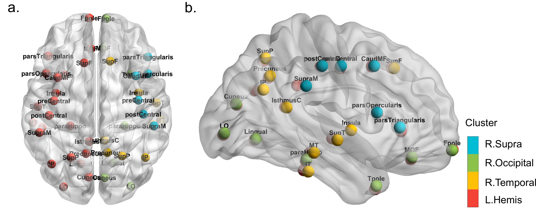
Refer to caption
Figure 9: Illustration of brain node clustering results for HCP data with (a) top and (b) side views.
Refer to caption
Figure 10: Mode 3 slices of estimated core tensor 𝒮^\hat{\mathcal{S}}. (a) Average estimated slice weighted by the group size; (b)-(d) Group-specified enrichment, i.e., the difference between each slice of 𝒮^\hat{\mathcal{S}} and the averaged slice.
Refer to caption
Figure 11: Observed brain connections in the population and each group of individuals. (a) Average brain network; (b)-(d) Group-specified brain network enrichments in Groups 1-3. Red edges represent the positive enrichment and blue edges represent the negative enrichment.

Figure 10 illustrates the estimated core tensor 𝒮^\hat{\mathcal{S}} with estimated clustering, and Figure 11 visualizes the average brain connections and the connection enrichment in contrast to average networks in each group. In general, we find that the inner-hemisphere connection has stronger connection compared to inter-hemisphere connections (Figure 10a). Also, the back and front parts (R.Occipital, R.Supra) are shown to have more interactions with temporal tissues than inner-cluster connections. In addition, the group 1 with 54% females shows an enrichment on the inter-hemisphere connections (Figure 10b), while group 4 with only 36% females exhibits a reduction (Figure 10d). This result agrees with previous findings in Hu et al., 2022. The enrichment on the back-front connection is also recognized in group 3 (Figure 10c). The interpretive patterns in our results demonstrate the usefulness of our clustering methods in the human brain connectome data application.

7.2 Peru Legislation data analysis

We also apply our method to the legislation networks in the Congress of the Republic of Peru (Lee et al., 2017). Because of the frequent political power shifts in the Peruvian Congress during 2006-2011, we choose to focus on the data for the first half of 2006-2007 year. The dataset records the co-sponsorship of 116 legislators from top 5 parties and 802 bill proposals. We reconstruct legislation network as an order-3 binary tensor 𝒴∈{0,1}116×116×116\mathcal{Y}\in\{0,1\}^{116\times 116\times 116}, where 𝒴i​j​k=1\mathcal{Y}_{ijk}=1 if the legislators (i,j,k)(i,j,k) have sponsored the same bill, and 𝒴i​j​k=0\mathcal{Y}_{ijk}=0 otherwise. The true party affiliations of legislators are provided and serve as the ground truth. We apply various higher-order clustering methods to 𝒴\mathcal{Y} with r=5r=5. Table 4 shows that our dTBM achieves the best performance compared to others. The second best method is the two-stage algorithm HLloyd, followed by the spectral methods SCORE and HOSVD+. This result is consistent with our simulations under strong signal and moderate degree heterogeneity. The comparison suggests that our method dTBM is more appealing in real-world applications.

Method dTBM HOSVD HOSVD+ HLloyd SCORE
CER 0.116 0.22 0.213 0.149 0.199
Table 4: Clustering errors (measured by CER) for various methods in the analysis of Peru Legislation dataset.

8 Proof Sketches

In this section, we provide the proof sketches for the main Theorem 2 (Impossibility), Theorem 3 (Impossibility), and Theorems 4-5. Detail proofs and extra theoretical results are provided in Appendix B.

8.1 Proof sketches of Theorems 2 and 3 (Impossibility)

The proofs of impossibility in Theorems 2 and 3 share the same proof idea with Han et al., 2022a and Gao et al., 2018. In both proofs of statistical and computational impossibilities, the key idea is to construct a particular set of parameters to lower bound the minimax rate. Specifically, for statistical impossibility in Theorem 2, we construct a particular (zstats∗,𝜽stats∗)∈𝒫z,𝜽(z^{*}_{\rm stats},\bm{\theta}^{*}_{\rm stats})\in\mathcal{P}_{z,\bm{\theta}} such that for all 𝒮∗∈𝒫𝒮​(γ)\mathcal{S}^{*}\in\mathcal{P}_{\mathcal{S}}(\gamma)

infz^statssup(z,𝜽)∈𝒫z,𝜽𝔼⁡[p​ℓ​(z^stat,z)]≥infz^stats𝔼⁡[p​ℓ​(z^stat,zstats∗)|(zstats∗,𝒮∗,𝜽stats∗)]≥1;\displaystyle\inf_{\hat{z}_{\rm stats}}\sup_{(z,\bm{\theta})\in\mathcal{P}_{z,\bm{\theta}}}\mathbb{E}[p\ell(\hat{z}_{\rm stat},z)]\geq\inf_{\hat{z}_{\rm stats}}\mathbb{E}[p\ell(\hat{z}_{\rm stat},z_{\rm stats}^{*})|(z^{*}_{\rm stats},\mathcal{S}^{*},\bm{\theta}^{*}_{\rm stats})]\geq 1; (66)

for computational impossibility in Theorem 3, we construct a particular (zcomp∗,𝒮comp∗,𝜽comp∗)∈𝒫⁡(γ)(z^{*}_{\rm comp},\mathcal{S}^{*}_{\rm comp},\bm{\theta}^{*}_{\rm comp})\in\mathcal{P}(\gamma) such that

infz^compsup(z,𝒮,𝜽)∈𝒫⁡(γ)𝔼⁡[p​ℓ​(z^comp,z)]≥infz^comp𝔼⁡[p​ℓ​(z^comp,zcomp∗)|(zcomp∗,𝒮comp∗,𝜽comp∗)]≥1.\displaystyle\inf_{\hat{z}_{\rm comp}}\sup_{(z,\mathcal{S},\bm{\theta})\in\mathcal{P}(\gamma)}\mathbb{E}[p\ell(\hat{z}_{\rm comp},z)]\geq\inf_{\hat{z}_{\rm comp}}\mathbb{E}[p\ell(\hat{z}_{\rm comp},z_{\rm comp}^{*})|(z^{*}_{\rm comp},\mathcal{S}^{*}_{\rm comp},\bm{\theta}^{*}_{\rm comp})]\geq 1. (67)

The constructions of (zstats∗,𝜽stats∗)(z^{*}_{\rm stats},\bm{\theta}^{*}_{\rm stats}) and (zcomp∗,𝒮comp∗,𝜽comp∗)(z^{*}_{\rm comp},\mathcal{S}^{*}_{\rm comp},\bm{\theta}^{*}_{\rm comp}) are the most critical steps. With good constructions, the lower bound “≥1\geq 1” can be verified by classical statistical conclusions (e.g. Neyman-Pearson Lemma) or prior work (e.g. HPC Conjecture).

A notable detail in the proof of statistical impossibility is the arbitrariness of 𝒮∗\mathcal{S}^{*}. The first infimum over 𝒫𝒮​(γ)\mathcal{P}_{\mathcal{S}}(\gamma) in the minimax rate (23) requires that the lower bound (66) holds for any 𝒮∗∈𝒫𝒮​(γ)\mathcal{S}^{*}\in\mathcal{P}_{\mathcal{S}}(\gamma). The arbitrary choice of 𝒮∗\mathcal{S}^{*} brings extra difficulties in the parameter construction, and consequently a non-trivial 𝜽stats∗≠𝟏\bm{\theta}^{*}_{\rm stats}\neq\mathbf{1} is chosen to address the arbitrariness. Previous TBM construction in the proof of Han et al., 2022a with 𝜽stats∗=𝟏\bm{\theta}^{*}_{\rm stats}=\mathbf{1} is no longer applicable in our case. Meanwhile, our construction (zcomp∗,𝒮comp∗,𝜽comp∗)(z^{*}_{\rm comp},\mathcal{S}^{*}_{\rm comp},\bm{\theta}^{*}_{\rm comp}) leads to a rank-2 mean tensor to relate the HPC Conjecture while TBM Han et al., 2022a constructs a rank-1 mean tensor. Hence, we emphasize that dTBM-specific techniques are required to obtain our impossibility results, though the proof idea is common for minimax lower bound analysis.

8.2 Proof sketch of Theorem 4

The proof of Theorem 4 is inspired by the proof idea of Gao et al., 2018. The extra difficulties are the angle gap characterization and multilinear algebra property in tensors; we address both challenges in our proof. Specifically, we control the misclustering error by the estimation error of 𝒳^\hat{\mathcal{X}} calculated in Step 2 of Sub-algorithm 1. We prove the following inequality

ℓ⁡(z(0),z)\displaystyle\ell(z^{(0)},z) ≲1pminπ∈Π∑i:z(0)​(i)≠π⁡(z⁡(i))θ(i)2≲σ2​rK−1Δmin2​pK∥𝒳^−𝒳∥F2≲rKp−K/2SNR,\displaystyle\lesssim\frac{1}{p}\min_{\pi\in\Pi}\sum_{i:z^{(0)}(i)\neq\pi(z(i))}\theta(i)^{2}\lesssim\frac{\sigma^{2}r^{K-1}}{\Delta_{\min}^{2}p^{K}}\lVert\hat{\mathcal{X}}-\mathcal{X}\rVert_{F}^{2}\lesssim\frac{r^{K}p^{-K/2}}{\text{SNR}}, (68)

where 𝒳=𝔼​𝒴\mathcal{X}=\mathbb{E}\mathcal{Y} is the true mean. The first inequality in (68) holds with the assumption mini∈[p]⁡θ⁡(i)≥c>0\min_{i\in[p]}\theta(i)\geq c>0 in Theorem 4. The second inequality relies on the key Lemma 1, which indicates

minz⁡(i)≠z⁡(j)∥[𝑿i:]s−[𝑿j:]s∥≳Δmin,\min_{z(i)\neq z(j)}\lVert[\bm{X}_{i:}]^{s}-[\bm{X}_{j:}]^{s}\rVert\gtrsim\Delta_{\min}, (69)

where 𝑿=Mat​(𝒳)\bm{X}=\text{Mat}(\mathcal{X}). The most challenging part in the proof of Theorem 4 lies in the derivation of inequality (69) (or the proof of Lemma 1), in which the proof of Gao et al., 2018 is no longer applicable due to different angle gap assumption in our dTBM. To address the angle gap notion, we develop the extra padding technique in Lemma 5 and balance assumption (17). Last, we finish the proof of Theorem 4 by showing the third inequality of (68) using Han et al., 2022a.

8.3 Proof sketch of Theorem 5

The proof of Theorem 5 is inspired by the proof idea of Han et al., 2022a. We develop extra polar-coordinate based techniques with angle gap characterization to address the nuisance degree heterogeneity. Recall the intermediate quantity, misclustering loss, defined in (32)

L(t):=L(z,z(t))=1p∑i∈[p]θ(i)∑b∈[r]𝟙{z(t)(i)=b}‖[𝑺z⁡(i):]s−[𝑺b:]s‖2.\displaystyle L^{(t)}:=L(z,z^{(t)})=\frac{1}{p}\sum_{i\in[p]}\theta(i)\sum_{b\in[r]}\mathds{1}\left\{z^{(t)}(i)=b\right\}\left\lVert\left[\bm{S}_{z(i):}\right]^{s}-\left[\bm{S}_{b:}\right]^{s}\right\rVert^{2}. (70)

We show that L(t)L^{(t)} provides an upper bound for the misclustering error of interest via the inequality ℓ(t)≤L(t)Δmin2\ell^{(t)}\leq{L^{(t)}\over\Delta^{2}_{\min}} in Lemma 2. Therefore, it suffices to control L(t)L^{(t)}. Further, we introduce the oracle estimators for core tensor under the true cluster assignment via

𝒮~=𝒴×1𝑾T×2⋯×K𝑾T,\tilde{\mathcal{S}}=\mathcal{Y}\times_{1}\bm{W}^{T}\times_{2}\cdots\times_{K}\bm{W}^{T}, (71)

where 𝑾=𝑴​(diag​(𝟏pT​𝑴))−1\bm{W}=\bm{M}\left(\text{diag}(\mathbf{1}_{p}^{T}\bm{M})\right)^{-1} is the weighted true membership matrix. Let 𝑽=𝑾⊗(K−1)\bm{V}=\bm{W}^{\otimes(K-1)} denote the Kronecker product of (K−1)(K-1) copies of 𝑾\bm{W} matrices, and we define the tt-th iteration quantities 𝑾(t),𝑽(t)\bm{W}^{(t)},\bm{V}^{(t)} corresponding to 𝑴(t)\bm{M}^{(t)} (or equivalently z(t)z^{(t)}). To evaluate L(t+1)L^{(t+1)}, we prove the bound

𝟙{z(t+1)(i)=b}=𝟙{∥[𝒀i:𝑽(t)]s−[𝑺b:(t)]s∥2≤∥[𝒀i:𝑽(t)]s−[𝑺z⁡(i):(t)]s∥2}≤Ai​b+Bi​b,\displaystyle\mathds{1}\left\{z^{(t+1)}(i)=b\right\}=\mathds{1}\left\{\lVert[\bm{Y}_{i:}\bm{V}^{(t)}]^{s}-[\bm{S}_{b:}^{(t)}]^{s}\rVert^{2}\leq\lVert[\bm{Y}_{i:}\bm{V}^{(t)}]^{s}-[\bm{S}_{z(i):}^{(t)}]^{s}\rVert^{2}\right\}\leq A_{ib}+B_{ib}, (72)

where 𝒀=Mat​(𝒴)\bm{Y}=\text{Mat}(\mathcal{Y}), 𝑺=Mat​(𝒮)\bm{S}=\text{Mat}(\mathcal{S}), 𝑺(t)=Mat​(𝒮(t))\bm{S}^{(t)}=\text{Mat}(\mathcal{S}^{(t)}) and

Ai​b\displaystyle A_{ib} =𝟙{⟨𝑬i:𝑽,[𝑺~z⁡(i):]s−[𝑺~b:]s⟩≲−‖[𝑺z⁡(i):]s−[𝑺b:]s‖2},\displaystyle=\mathds{1}\left\{\left\langle\bm{E}_{i:}\bm{V},\left[\tilde{\bm{S}}_{z(i):}\right]^{s}-\left[\tilde{\bm{S}}_{b:}\right]^{s}\right\rangle\lesssim-\left\lVert\left[\bm{S}_{z(i):}\right]^{s}-\left[\bm{S}_{b:}\right]^{s}\right\rVert^{2}\right\}, (73)
Bi​b\displaystyle B_{ib} =𝟙{‖[𝑺z⁡(i):]s−[𝑺b:]s‖2≲Fi​b(t)+Gi​b(t)+Hi​b(t)}.\displaystyle=\mathds{1}\left\{\left\lVert\left[\bm{S}_{z(i):}\right]^{s}-\left[\bm{S}_{b:}\right]^{s}\right\rVert^{2}\lesssim F_{ib}^{(t)}+G_{ib}^{(t)}+H_{ib}^{(t)}\right\}. (74)

The terms Fi​b(t),Gi​b(t),Hi​b(t)F_{ib}^{(t)},G_{ib}^{(t)},H_{ib}^{(t)} are controlled by z(t),𝒮(t)z^{(t)},\mathcal{S}^{(t)}; see the detailed definitions in (235), (237), (238). Note that the event Ai​bA_{ib} only involves the oracle estimator independent of tt, while all the terms related to the tt-th iteration are in Bi​bB_{ib}. Thus, the inequality (72) decomposes the misclustering loss in the (t+1)(t+1)-th iteration into the oracle loss and the loss in tt-th iteration. This decomposition leads to the separation of statistical error and computational error in the final upper bound of Theorem 5.

Specifically, we prove the contraction inequality

L(t+1)≤Mξ+ρL(t), with ξ=1p∑i∈[p]θ(i)∑b∈[r]Ai​b‖[𝑺z⁡(i):]s−[𝑺b:]s‖2,\displaystyle L^{(t+1)}\leq M\xi+\rho L^{(t)},\text{ with }\xi=\frac{1}{p}\sum_{i\in[p]}\theta(i)\sum_{b\in[r]}A_{ib}\left\lVert\left[\bm{S}_{z(i):}\right]^{s}-\left[\bm{S}_{b:}\right]^{s}\right\rVert^{2}, (75)

where MM is a positive constant, ρ∈(0,1)\rho\in(0,1) is the contraction parameter, and we call ξ\xi the oracle loss. Controlling the probability of event Bi​bB_{ib} and obtaining the ρ​L(t)\rho L^{(t)} term in the right hand side of (75) are the most challenging parts in the proof of Theorem 5. Note that the true and estimated core tensors are involved via their normalized rows such as 𝑺a:s,𝑺~a:s,[𝑺a:(t)]s\bm{S}_{a:}^{s},\tilde{\bm{S}}_{a:}^{s},[\bm{S}^{(t)}_{a:}]^{s}. The Cartesian coordinate based analysis in Han et al., 2022a is no longer applicable in our case. Instead, we use the polar-coordinate based analysis and the geometry property of trigonometric functions to derive the high probability upper bounds for Fi​b(t),Gi​b(t),Hi​b(t)F_{ib}^{(t)},G_{ib}^{(t)},H_{ib}^{(t)}.

Further, by sub-Gaussian concentration, we prove the high probability upper bound for oracle loss

ξ≲SNR−1​exp⁡(−pK−1​SNRrK−1).\xi\lesssim{\text{SNR}^{-1}}\exp\left(-\frac{p^{K-1}\text{SNR}}{r^{K-1}}\right). (76)

Combining the decomposition (75) and the oracle bound (76), we finish the proof of Theorem 5.

The proof of MLE error shares the similar idea as Theorems 4-5. We first show a weaker polynomial rate for MLE and then improve the rate from polynomial to exponential through the iterations. The only difference is that the MLE remains the same over iterations due to its global optimality. See Appendix B, Section B.10 for the detailed proof.

Acknowledgment

This research is supported in part by NSF CAREER DMS-2141865, DMS-1915978, DMS-2023239, EF-2133740, and funding from the Wisconsin Alumni Research foundation. We thank Zheng Tracy Ke, Anru Zhang, Rungang Han, Yuetian Luo for helpful discussions and for sharing software packages.

References

  • Abbe, (2018) Abbe, E. (2018). Community detection and stochastic block models: Recent developments. Journal of Machine Learning Research, 18(177):1–86.
  • Abbe et al., (2020) Abbe, E., Fan, J., Wang, K., and Zhong, Y. (2020). Entrywise eigenvector analysis of random matrices with low expected rank. The Annals of Statistics, 48(3):1452–1474.
  • Ahn et al., (2018) Ahn, K., Lee, K., and Suh, C. (2018). Hypergraph spectral clustering in the weighted stochastic block model. IEEE Journal of Selected Topics in Signal Processing, 12(5):959–974.
  • Ahn et al., (2019) Ahn, K., Lee, K., and Suh, C. (2019). Community recovery in hypergraphs. IEEE Transactions on Information Theory, 65(10):6561–6579.
  • Anandkumar et al., (2014) Anandkumar, A., Ge, R., Hsu, D., Kakade, S. M., and Telgarsky, M. (2014). Tensor decompositions for learning latent variable models. Journal of Machine Learning Research, 15(80):2773–2832.
  • Bickel and Chen, (2009) Bickel, P. J. and Chen, A. (2009). A nonparametric view of network models and newman–girvan and other modularities. Proceedings of the National Academy of Sciences, 106(50):21068–21073.
  • Brennan and Bresler, (2020) Brennan, M. and Bresler, G. (2020). Reducibility and statistical-computational gaps from secret leakage. In Proceedings of Thirty Third Conference on Learning Theory, volume 125, pages 648–847.
  • Chi et al., (2020) Chi, E. C., Gaines, B. J., Sun, W. W., Zhou, H., and Yang, J. (2020). Provable convex co-clustering of tensors. Journal of Machine Learning Research, 21(214):1–58.
  • Chi et al., (2019) Chi, Y., Lu, Y. M., and Chen, Y. (2019). Nonconvex optimization meets low-rank matrix factorization: An overview. IEEE Transactions on Signal Processing, 67(20):5239–5269.
  • Chien et al., (2019) Chien, I. E., Lin, C.-Y., and Wang, I.-H. (2019). On the minimax misclassification ratio of hypergraph community detection. IEEE Transactions on Information Theory, 65(12):8095–8118.
  • De Lathauwer et al., (2000) De Lathauwer, L., De Moor, B., and Vandewalle, J. (2000). A multilinear singular value decomposition. SIAM Journal on Matrix Analysis and Applications, 21(4):1253–1278.
  • Desikan et al., (2006) Desikan, R. S., Ségonne, F., Fischl, B., Quinn, B. T., Dickerson, B. C., Blacker, D., Buckner, R. L., Dale, A. M., Maguire, R. P., Hyman, B. T., Albert, M. S., and Killiany, R. J. (2006). An automated labeling system for subdividing the human cerebral cortex on MRI scans into gyral based regions of interest. Neuroimage, 31:968–980.
  • Florescu and Perkins, (2016) Florescu, L. and Perkins, W. (2016). Spectral thresholds in the bipartite stochastic block model. In Proceedings of Twenty Ninth Conference on Learning Theory, volume 49, pages 943–959.
  • Gao et al., (2018) Gao, C., Ma, Z., Zhang, A. Y., and Zhou, H. H. (2018). Community detection in degree-corrected block models. The Annals of Statistics, 46(5):2153–2185.
  • Gao and Zhang, (2022) Gao, C. and Zhang, A. Y. (2022). Iterative algorithm for discrete structure recovery. The Annals of Statistics, 50(2):1066–1094.
  • Ghoshdastidar and Dukkipati, (2017) Ghoshdastidar, D. and Dukkipati, A. (2017). Uniform hypergraph partitioning: Provable tensor methods and sampling techniques. Journal of Machine Learning Research, 18(50):1–41.
  • Ghoshdastidar et al., (2017) Ghoshdastidar, D. et al. (2017). Consistency of spectral hypergraph partitioning under planted partition model. The Annals of Statistics, 45(1):289 – 315.
  • (18) Han, R., Luo, Y., Wang, M., and Zhang, A. R. (2022a). Exact clustering in tensor clock model: Statistical optimality and computational limit. Journal of the Royal Statistical Society: Series B (Statistical Methodology), 84(5):1666–1698.
  • (19) Han, R., Willett, R., and Zhang, A. R. (2022b). An optimal statistical and computational framework for generalized tensor estimation. The Annals of Statistics, 50(1):1–29.
  • Hore et al., (2016) Hore, V., Viñuela, A., Buil, A., Knight, J., McCarthy, M. I., Small, K., and Marchini, J. (2016). Tensor decomposition for multiple-tissue gene expression experiments. Nature genetics, 48(9):1094.
  • Hu et al., (2022) Hu, J., Lee, C., and Wang, M. (2022). Generalized tensor decomposition with features on multiple modes. Journal of Computational and Graphical Statistics, 31(1):204–218.
  • Ke et al., (2019) Ke, Z. T., Shi, F., and Xia, D. (2019). Community detection for hypergraph networks via regularized tensor power iteration. arXiv preprint arXiv:1909.06503.
  • Kim et al., (2018) Kim, C., Bandeira, A. S., and Goemans, M. X. (2018). Stochastic block model for hypergraphs: Statistical limits and a semidefinite programming approach. arXiv preprint arXiv:1807.02884.
  • Koniusz and Cherian, (2016) Koniusz, P. and Cherian, A. (2016). Sparse coding for third-order super-symmetric tensor descriptors with application to texture recognition. In Proceedings of the IEEE Conference on Computer Vision and Pattern Recognition, pages 5395–5403.
  • Lee et al., (2017) Lee, S. H., Magallanes, J. M., and Porter, M. A. (2017). Time-dependent community structure in legislation cosponsorship networks in the congress of the republic of peru. Journal of Complex Networks, 5(1):127–144.
  • Lu and Zhou, (2016) Lu, Y. and Zhou, H. H. (2016). Statistical and computational guarantees of lloyd’s algorithm and its variants. arXiv preprint arXiv:1612.02099.
  • Meilă, (2012) Meilă, M. (2012). Local equivalences of distances between clusterings—a geometric perspective. Machine Learning, 86(3):369–389.
  • Mu et al., (2014) Mu, C., Huang, B., Wright, J., and Goldfarb, D. (2014). Square deal: Lower bounds and improved relaxations for tensor recovery. In Proceedings of the 31st International Conference on Machine Learning, volume 32, pages 73–81.
  • Rigollet and Hütter, (2015) Rigollet, P. and Hütter, J.-C. (2015). High dimensional statistics. Lecture notes for course 18S997.
  • Van Essen et al., (2013) Van Essen, D. C., Smith, S. M., Barch, D. M., Behrens, T. E., Yacoub, E., Ugurbil, K., and WU-Minn HCP Consortium (2013). The WU-Minn human connectome project: An overview. Neuroimage, 80:62–79.
  • Wang et al., (2017) Wang, L., Durante, D., Jung, R. E., and Dunson, D. B. (2017). Bayesian network–response regression. Bioinformatics, 33(12):1859–1866.
  • Wang et al., (2019) Wang, M., Fischer, J., and Song, Y. S. (2019). Three-way clustering of multi-tissue multi-individual gene expression data using semi-nonnegative tensor decomposition. The Annals of Applied Statistics, 13(2):1103–1127.
  • Wang and Zeng, (2019) Wang, M. and Zeng, Y. (2019). Multiway clustering via tensor block models. In Advances in Neural Information Processing Systems, volume 32.
  • Yuan et al., (2022) Yuan, M., Liu, R., Feng, Y., and Shang, Z. (2022). Testing community structure for hypergraphs. The Annals of Statistics, 50(1):147–169.
  • Yun and Proutiere, (2016) Yun, S.-Y. and Proutiere, A. (2016). Optimal cluster recovery in the labeled stochastic block model. In Advances in Neural Information Processing Systems, volume 29.
  • Zhang and Xia, (2018) Zhang, A. and Xia, D. (2018). Tensor SVD: Statistical and computational limits. IEEE Transactions on Information Theory, 64(11):7311–7338.
  • Zhang et al., (2019) Zhang, Z., Allen, G. I., Zhu, H., and Dunson, D. (2019). Tensor network factorizations: Relationships between brain structural connectomes and traits. Neuroimage, 197:330–343.

Appendices

A Additional numerical experiments

Bernoulli phase transition. The first additional experiment verifies the statistical-computational gap in Section 3 under the Bernoulli model. Consider the Bernoulli model with p={80,100}p=\{80,100\}, r=5r=5. We vary γ\gamma in [−1.2,−0.4][-1.2,-0.4] and [−2.1,−1.4][-2.1,-1.4] for matrix (K=2K=2) and tensor (K=3)(K=3) clustering, respectively. We approximate MLE using an oracle estimator, i.e., the output of Sub-algorithm 2 initialized from the true assignment. Figure 12 shows a similar pattern as Figure 4. The algorithm and oracle estimators have no gap in the matrix case, while an error gap emerges between the critical values γstat=−2\gamma_{\text{stat}}=-2 and γcomp=−1.5\gamma_{\text{comp}}=-1.5 in the tensor case. Figure 4 suggests the statistical-computational gap in Bernoulli models.

Figure 12: SNR phase transitions for Bernoulli dTBM with p={80,100},r=5p=\{80,100\},r=5 under (a) matrix case with γ∈[−1.2,−0.4]\gamma\in[-1.2,-0.4] and (b) tensor case with γ∈[−2.1,−1.4]\gamma\in[-2.1,-1.4].

Sparsity. The second additional experiment evaluates the algorithm performances under the sparse binary dTBM (54). We fix the signal exponent γ=−1.2\gamma=-1.2 and vary the sparsity parameter αp∈[0.05,0.9]\alpha_{p}\in[0.05,0.9]. A smaller αp\alpha_{p} leads to a higher probability of zero entries in the observation. In addition to the three algorithms mentioned in Section 6.2 (denoted Initialization, dTBM, and SCORE), we consider other three algorithms based on the discussion in Section 4.3:

  • •

    D-HOSVD, the diagonal-deleted HOSVD in Ke et al., 2019;

  • •

    D-HOSVD + Angle, the combined algorithm of our angle-based iteration with initialization from D-HOSVD;

  • •

    SCORE + Angle, the combined algorithms of our angle-based iteration with initialization from SCORE.

Figure 13: CER comparison versus sparsity parameter αp\alpha_{p} in [0.05,0.9][0.05,0.9]. We set p=100,r=5p=100,r=5 and γ=−1.2\gamma=-1.2 under sparse binary dTBM.

Figure 13 shows a slightly larger error in dTBM than that in SCORE, D-HOSVD + Angle, and SCORE + Angle under the sparse setting with αp<0.3\alpha_{p}<0.3. The small gap between dTBM and other sparse-specific methods implies the robustness of our algorithm. In addition, comparing SCORE versus SCORE + Angle (or D-HOSVD versus D-HOSVD + Angle) indicates the benefit of our angle iterations under the sparse dTBM. In the intermediate and dense cases with αp≥0.3\alpha_{p}\geq 0.3, our proposed dTBM has a clear improvement over others, which again verifies the success of our algorithm in dense settings.

B Proofs

We provide the proofs for all the theorems in our main paper. In each sub-section, we first show the proof of main theorem and then collect the useful lemmas in the end. We combine the proofs of MLE achievement in Theorem 2 and polynomial-time achievement in Theorem 5 in the last section due to the similar idea.

B.4 Notation

Before the proofs, we first introduce the notation used throughout the appendix and the general dTBM without symmetric assumptions. The parameter space and minimal gap assumption are also extended for the general asymmetric dTBM.

Preliminaries.

  1. 1.

    For mode k∈[K]k\in[K], denote mode-kk tensor matricizations by

    𝒀k=Matk​(𝒴),𝑺k=Matk​(𝒮),𝑬k=Matk​(ℰ),𝑿k=Matk​(𝒳).\displaystyle\bm{Y}_{k}=\text{Mat}_{k}\left(\mathcal{Y}\right),\quad\bm{S}_{k}=\text{Mat}_{k}\left(\mathcal{S}\right),\quad\bm{E}_{k}=\text{Mat}_{k}\left(\mathcal{E}\right),\quad\bm{X}_{k}=\text{Mat}_{k}\left(\mathcal{X}\right). (77)
  2. 2.

    For a vector 𝒂\bm{a}, let 𝒂s≔𝒂/‖𝒂‖\bm{a}^{s}\coloneqq\bm{a}/\left\lVert\bm{a}\right\rVert denote the normalized vector. We make the convention that 𝒂s=𝟎\bm{a}^{s}={\bf 0} if 𝒂=𝟎\bm{a}={\bf 0}.

  3. 3.

    For a matrix 𝑨∈ℝn×m\bm{A}\in\mathbb{R}^{n\times m}, let 𝑨⊗K:=𝑨⊗⋯⊗𝑨∈ℝnK×mK\bm{A}^{\otimes K}:=\bm{A}\otimes\cdots\otimes\bm{A}\in\mathbb{R}^{n^{K}\times m^{K}} denote the Kronecker product of KK copies of matrices 𝑨\bm{A}.

  4. 4.

    For a matrix 𝑨\bm{A}, let ∥𝑨∥σ\lVert\bm{A}\rVert_{\sigma} denote the spectral norm of matrix 𝑨\bm{A}, which is equal to the maximal singular value of 𝑨\bm{A}; let λk​(𝑨)\lambda_{k}(\bm{A}) denote the kk-th largest singular value of 𝑨\bm{A}; let ∥𝑨∥F\lVert\bm{A}\rVert_{F} denote the Frobenius norm of matrix 𝑨\bm{A}.

Extension to general asymmetric dTBM.

The general order-KK (p1,…,pK)(p_{1},\ldots,p_{K})-dimensional dTBM with rkr_{k} communities and degree heterogeneity 𝜽k=⟦θk​(i)⟧∈ℝ+pk\bm{\theta}_{k}=\llbracket\theta_{k}(i)\rrbracket\in\mathbb{R}_{+}^{p_{k}} is represented by

𝒴=𝒳+ℰ,where𝒳=𝒮×1𝚯1𝑴1×2⋯×K𝚯K𝑴K,\mathcal{Y}=\mathcal{X}+\mathcal{E},\ \text{where}\ \mathcal{X}=\mathcal{S}\times_{1}\bm{\Theta}_{1}\bm{M}_{1}\times_{2}\cdots\times_{K}\bm{\Theta}_{K}\bm{M}_{K}, (78)

where 𝒴∈ℝp1×⋯×pK\mathcal{Y}\in\mathbb{R}^{p_{1}\times\cdots\times p_{K}} is the data tensor, 𝒳∈ℝp1×⋯×pK\mathcal{X}\in\mathbb{R}^{p_{1}\times\cdots\times p_{K}} is the mean tensor, 𝒮∈ℝr1×⋯×rK\mathcal{S}\in\mathbb{R}^{r_{1}\times\cdots\times r_{K}} is the core tensor, ℰ∈ℝp1×⋯×pK\mathcal{E}\in\mathbb{R}^{p_{1}\times\cdots\times p_{K}} is the noise tensor consisting of independent zero-mean sub-Gaussian entries with variance bounded by σ2\sigma^{2}, 𝚯k=diag​(𝜽k)\bm{\Theta}_{k}=\text{diag}(\bm{\theta}_{k}), and 𝑴k∈{0,1}pk×rk\bm{M}_{k}\in\{0,1\}^{p_{k}\times r_{k}} is the membership matrix corresponding to the assignment zk:[pk]↦[rk]z_{k}:[p_{k}]\mapsto[r_{k}], for all k∈[K]k\in[K].

For ease of notation, we use {zk}\{z_{k}\} to denote the collection {zk}k=1K\{z_{k}\}_{k=1}^{K}, and {𝜽k}\{\bm{\theta}_{k}\} to denote the collection {𝜽k}k=1K\{\bm{\theta}_{k}\}_{k=1}^{K}. Correspondingly, we consider the parameter space for the triplet ({zk},𝒮,{𝜽k})\left(\{z_{k}\},\mathcal{S},\{\bm{\theta}_{k}\}\right),

𝒫({rk})={\displaystyle\mathcal{P}(\{r_{k}\})=\Big\{ ({zk},𝒮,{𝜽k}):𝜽k∈ℝ+p,c1​pkrk​|zk−1​(a)|≤c2​pkrk,\displaystyle\left(\{z_{k}\},\mathcal{S},\{\bm{\theta}_{k}\}\right):\bm{\theta}_{k}\in\mathbb{R}^{p}_{+},{c_{1}p_{k}\over r_{k}}|z_{k}^{-1}(a)|\leq{c_{2}p_{k}\over r_{k}}, (79)
c3≤‖𝑺k,a:‖≤c4,∥𝜽k,zk−1​(a)∥1=|zk−1(a)|,for all a∈[rk],k∈[K]}.\displaystyle c_{3}\leq\left\lVert\bm{S}_{k,a:}\right\rVert\leq c_{4},\lVert\bm{\theta}_{k,z_{k}^{-1}(a)}\rVert_{1}=|z_{k}^{-1}(a)|,\text{for all }a\in[r_{k}],k\in[K]\Big\}. (80)

We call the degree heterogeneity {𝜽k}\{\bm{\theta}_{k}\} is balanced if for all k∈[K]k\in[K],

mina∈[r]⁡∥𝜽k,zk−1​(a)∥=(1+o⁡(1))​maxa∈[r]​∥𝜽k,zk−1​(a)∥.{\min_{a\in[r]}\lVert\bm{\theta}_{k,z_{k}^{-1}(a)}\rVert=\left(1+o(1)\right)\max_{a\in[r]}\lVert\bm{\theta}_{k,z_{k}^{-1}(a)}\rVert}. (81)

We also consider the generalized Assumption 1 on angle gap.

Assumption 2 (Generalized angle gap).

Recall 𝑺k=Matk​(𝒮)\bm{S}_{k}=\text{Mat}_{k}(\mathcal{S}). We assume the minimal gap between normalized rows of 𝑺k\bm{S}_{k} is bounded away from zero for all k∈[K]k\in[K]; i.e.,

Δmin≔mink∈[K]mina≠b∈[rk]‖𝑺k,a:s−𝑺k,b:s‖>0.\Delta_{\min}\coloneqq\min_{k\in[K]}\min_{a\neq b\in[r_{k}]}\left\lVert\bm{S}_{k,a:}^{s}-\bm{S}_{k,b:}^{s}\right\rVert>0. (82)

Similarly, let SNR=Δmin2/σ2\text{SNR}=\Delta_{\min}^{2}/\sigma^{2} with the generalized minimal gap Δmin2\Delta_{\min}^{2} defined in Assumption 2. We define the regime

𝒫⁡(γ)=𝒫⁡({rk})∩{𝒮​ satisfies SNR=pγ and pk≍p,k∈[K]}.\displaystyle\mathcal{P}(\gamma)=\mathcal{P}(\{r_{k}\})\cap\{\mathcal{S}\text{ satisfies $\text{SNR}=p^{\gamma}$ and $p_{k}\asymp p,k\in[K]$}\}. (83)

B.5 Proof of Theorem 1

Proof of Theorem 1.

To study the identifiability, we consider the noiseless model with ℰ=0\mathcal{E}=0. Assume that there exist two parameterizations satisfying

𝒳\displaystyle\mathcal{X} =𝒮×1Θ1𝑴1×2⋯×KΘK𝑴′K=𝒮′×1Θ′1𝑴′1×2⋯×KΘ′K𝑴′K,\displaystyle=\mathcal{S}\times_{1}\Theta_{1}\bm{M}_{1}\times_{2}\cdots\times_{K}\Theta_{K}\bm{M}^{\prime}_{K}=\mathcal{S}^{\prime}\times_{1}\Theta^{\prime}_{1}\bm{M}^{\prime}_{1}\times_{2}\cdots\times_{K}\Theta^{\prime}_{K}\bm{M}^{\prime}_{K}, (84)

where ({zk},𝒮,{𝜽k})∈𝒫⁡({rk})\left(\{z_{k}\},\mathcal{S},\{\bm{\theta}_{k}\}\right)\in\mathcal{P}(\{r_{k}\}) and ({zk′},𝒮′,{𝜽k′})∈𝒫⁡({rk′})\left(\{z^{\prime}_{k}\},\mathcal{S}^{\prime},\{\bm{\theta}^{\prime}_{k}\}\right)\in\mathcal{P}(\{r_{k}^{\prime}\}) are two sets of parameters. We prove the sufficient and necessary conditions separately.

  1. (⇐)(\Leftarrow)

    For the necessity, it suffices to construct two distinct parameters up to cluster label permutation, if the model (78) violates Assumption 2. Note that Δmin2=1\Delta_{\min}^{2}=1 when there exists k∈[K]k\in[K] such that rk=1r_{k}=1. Hence, we consider the case that rk≥2r_{k}\geq 2 for all k∈[K]k\in[K]. Without loss of generality, we assume ‖𝑺1,1:s−𝑺1,2:s‖=0\left\lVert\bm{S}_{1,1:}^{s}-\bm{S}_{1,2:}^{s}\right\rVert=0.

    By constraints in parameter space (80), neither 𝑺1,1:\bm{S}_{1,1:} nor 𝑺1,2:\bm{S}_{1,2:} is a zero vector. There exists a positive constant cc such that 𝑺1,1:=c𝑺1,2:\bm{S}_{1,1:}=c\bm{S}_{1,2:}. Thus, there exists a core tensor 𝒮0∈ℝr1−1×⋯×rK\mathcal{S}_{0}\in\mathbb{R}^{r_{1}-1\times\cdots\times r_{K}} such that

    𝒮=𝒮0×1𝑪​𝑹,\mathcal{S}=\mathcal{S}_{0}\times_{1}\bm{C}\bm{R}, (85)

    where 𝑪=diag​(1,c,1,…,1)∈ℝr1×r1\bm{C}=\text{diag}(1,c,1,...,1)\in\mathbb{R}^{r_{1}\times r_{1}} and

    𝑹=(10100𝟏r1−2)∈ℝr1×(r1−1).\bm{R}=\begin{pmatrix}1&0\\ 1&0\\ 0&\mathbf{1}_{r_{1}-2}\end{pmatrix}\in\mathbb{R}^{r_{1}\times(r_{1}-1)}. (86)

    Let 𝑫=diag​(1+c,1,…,1)∈ℝr1−1×r1−1\bm{D}=\text{diag}(1+c,1,...,1)\in\mathbb{R}^{r_{1}-1\times r_{1}-1}. Consider the parameterization 𝑴1′=𝑴1​𝑹,𝒮′=𝒮0×1𝑫,\bm{M}^{\prime}_{1}=\bm{M}_{1}\bm{R},\mathcal{S}^{\prime}=\mathcal{S}_{0}\times_{1}\bm{D}, and

    θ1′​(i)={11+c​θ1​(i)i∈z1−1​(1),c1+c​θ1​(i)i∈z1−1​(2),θ1​(i) otherwise,\theta^{\prime}_{1}(i)=\begin{cases}\frac{1}{1+c}\theta_{1}(i)&i\in z_{1}^{-1}(1),\\ \frac{c}{1+c}\theta_{1}(i)&i\in z_{1}^{-1}(2),\\ \theta_{1}(i)&\text{ otherwise},\end{cases} (87)

    and 𝑴k′=𝑴k,𝜽k′=𝜽k\bm{M}^{\prime}_{k}=\bm{M}_{k},\bm{\theta}^{\prime}_{k}=\bm{\theta}_{k} for all k=2,…,Kk=2,\ldots,K. Then we have constructed a triplet ({zk′},𝒮′,{𝜽k′})\left(\{z^{\prime}_{k}\},\mathcal{S}^{\prime},\{\bm{\theta}^{\prime}_{k}\}\right) that is distinct from ({zk},𝒮,{𝜽k})\left(\{z_{k}\},\mathcal{S},\{\bm{\theta}_{k}\}\right) up to label permutation.

  2. (⇒)(\Rightarrow)

    For the sufficiency, it suffices to show that all possible triplets ({zk′},𝒮′,{𝜽k′})\left(\{z^{\prime}_{k}\},\mathcal{S}^{\prime},\{\bm{\theta}^{\prime}_{k}\}\right) are identical to ({zk},𝒮,{𝜽k})\left(\{z_{k}\},\mathcal{S},\{\bm{\theta}_{k}\}\right) up to label permutation if the model (78) satisfies Assumption (2). We show the uniqueness of the three parameters, {𝑴k},{𝒮},{𝜽k}\{\bm{M}_{k}\},\{\mathcal{S}\},\{\bm{\theta}_{k}\} separately.

    First, we show the uniqueness of 𝑴k\bm{M}_{k} for all k∈[K]k\in[K]. When rk=1r_{k}=1, all possible 𝑴k\bm{M}_{k}’s are equal to the vector 𝟏pk{\bf 1}_{p_{k}}, and the uniqueness holds trivially. Hence, we consider the case that rk≥2r_{k}\geq 2. Without loss of generality, we consider k=1k=1 with r1≥2r_{1}\geq 2 and show the uniqueness of the first mode membership matrix; i.e., 𝑴1′=𝑴1​𝑷1\bm{M}^{\prime}_{1}=\bm{M}_{1}\bm{P}_{1} where 𝑷1\bm{P}_{1} is a permutation matrix. The conclusion for k≥2k\geq 2 can be showed similarly and thus omitted.

    Consider an arbitrary node pair (i,j)(i,j). If z1​(i)=z1​(j)z_{1}(i)=z_{1}(j), then we have ∥𝑿1,z1​(i):s−𝑿1,z1​(j):s∥=0\lVert\bm{X}_{1,z_{1}(i):}^{s}-\bm{X}_{1,z_{1}(j):}^{s}\rVert=0 and thus ∥(𝑺′)1,z1′​(i):s−(𝑺′)1,z1′​(j):s∥=0\lVert(\bm{S}^{\prime})_{1,z^{\prime}_{1}(i):}^{s}-(\bm{S}^{\prime})_{1,z^{\prime}_{1}(j):}^{s}\rVert=0 by Lemma 3. Then, by Assumption (2), we have z1′​(i)=z1′​(j)z^{\prime}_{1}(i)=z^{\prime}_{1}(j). Conversely, if z1​(i)≠z1​(j)z_{1}(i)\neq z_{1}(j), then we have ‖𝑿1,i:s−𝑿1,j:s‖≠0\left\lVert\bm{X}_{1,i:}^{s}-\bm{X}_{1,j:}^{s}\right\rVert\neq 0 and thus ‖(𝑺′)1,z1′​(i):s−(𝑺′)1,z1′​(j):s‖≠0\left\lVert(\bm{S}^{\prime})_{1,z^{\prime}_{1}(i):}^{s}-(\bm{S}^{\prime})_{1,z^{\prime}_{1}(j):}^{s}\right\rVert\neq 0 by Lemma 3. Hence, we have z1′​(i)≠z1′​(j)z^{\prime}_{1}(i)\neq z^{\prime}_{1}(j). Therefore, we have proven that z1′z^{\prime}_{1} is identical ziz_{i} up to label permutation.

    Next, we show the uniqueness of 𝜽k\bm{\theta}_{k} for all k∈[K]k\in[K] provided that zk=zk′z_{k}=z_{k}^{\prime}. Similarly, consider k=1k=1 only, and omit the procedure for k≥2k\geq 2.

    Consider an arbitrary j∈[p1]j\in[p_{1}] such that z1​(j)=az_{1}(j)=a. Then for all the nodes i∈z1−1​(a)i\in z_{1}^{-1}(a) in the same cluster of jj, we have

    𝑿1,z1​(i):𝑿1,z1​(j):=𝑿′1,z1​(i):𝑿′1,z1​(j):, which implies θ1​(j)θ1​(i)=θ1′​(j)θ1′​(i).\frac{\bm{X}_{1,z_{1}(i):}}{\bm{X}_{1,z_{1}(j):}}=\frac{\bm{X}^{\prime}_{1,z_{1}(i):}}{\bm{X}^{\prime}_{1,z_{1}(j):}},\text{ which implies }\frac{\theta_{1}(j)}{\theta_{1}(i)}=\frac{\theta^{\prime}_{1}(j)}{\theta^{\prime}_{1}(i)}. (88)

    Let θ1′​(j)=c​θ1​(j)\theta^{\prime}_{1}(j)=c\theta_{1}(j) for some positive constant cc. By equation (88), we have θ1′​(i)=c​θ1​(i)\theta^{\prime}_{1}(i)=c\theta_{1}(i) for all i∈z1−1​(a)i\in z_{1}^{-1}(a). By the constraint ({zk},𝒮′,{𝜽k′})∈𝒫⁡({rk})(\{z_{k}\},\mathcal{S}^{\prime},\{\bm{\theta}^{\prime}_{k}\})\in\mathcal{P}(\{r_{k}\}), we have

    ∑j∈z1−1​(a)θ1′​(j)=c​∑j∈z1−1​(a)θ1​(j)=1,\sum_{j\in z_{1}^{-1}(a)}\theta^{\prime}_{1}(j)=c\sum_{j\in z_{1}^{-1}(a)}\theta_{1}(j)=1, (89)

    which implies c=1c=1. Hence, we have proven 𝜽1=𝜽1′\bm{\theta}_{1}=\bm{\theta}^{\prime}_{1} provided that z1=z1′z_{1}=z^{\prime}_{1}.

    Last, we show the uniqueness of 𝒮\mathcal{S}; i.e., 𝒮′=𝒮×1𝑷−11×2⋯×K𝑷−1K\mathcal{S}^{\prime}=\mathcal{S}\times_{1}\bm{P}^{-1}_{1}\times_{2}\cdots\times_{K}\bm{P}^{-1}_{K}, where 𝑷k\bm{P}_{k}’s are permutation matrices for all k∈[K]k\in[K]. Provided zk′=zk,𝜽k′=𝜽kz^{\prime}_{k}=z_{k},\bm{\theta}^{\prime}_{k}=\bm{\theta}_{k}, we have 𝑴k′=𝑴k​𝑷k\bm{M}^{\prime}_{k}=\bm{M}_{k}\bm{P}_{k} and 𝚯k′=𝚯k\bm{\Theta}^{\prime}_{k}=\bm{\Theta}_{k} for all k∈[K]k\in[K].

    Let 𝑫k=[(𝚯k′​𝑴k′)T​(𝚯k′​𝑴k′)]−1​(𝚯k′​𝑴k′)T,k∈[K]\bm{D}_{k}=\left[(\bm{\Theta}^{\prime}_{k}\bm{M}^{\prime}_{k})^{T}(\bm{\Theta}^{\prime}_{k}\bm{M}^{\prime}_{k})\right]^{-1}(\bm{\Theta}^{\prime}_{k}\bm{M}^{\prime}_{k})^{T},k\in[K]. By the parameterization (84), we have

    𝒮′\displaystyle\mathcal{S}^{\prime} =𝒳×1𝑫1×2⋯×K𝑫K\displaystyle=\mathcal{X}\times_{1}\bm{D}_{1}\times_{2}\cdots\times_{K}\bm{D}_{K} (90)
    =𝒮×1𝑫1𝚯1𝑴1×1⋯×K𝑫K𝚯K𝑴K\displaystyle=\mathcal{S}\times_{1}\bm{D}_{1}\bm{\Theta}_{1}\bm{M}_{1}\times_{1}\cdots\times_{K}\bm{D}_{K}\bm{\Theta}_{K}\bm{M}_{K} (91)
    =𝒮×1𝑷−11×2⋯×K𝑷−1K.\displaystyle=\mathcal{S}\times_{1}\bm{P}^{-1}_{1}\times_{2}\cdots\times_{K}\bm{P}^{-1}_{K}. (92)

Therefore, we finish the proof of Theorem 1. ∎

Useful Lemma for the Proof of Theorem 1

Lemma 3 (Motivation of angle-based clustering).

Consider the signal tensor 𝒳\mathcal{X} in the general asymmetric dTBM (78) with ({zk},𝒮,{𝜽k})∈𝒫⁡({rk})(\{z_{k}\},\mathcal{S},\{\bm{\theta}_{k}\})\in\mathcal{P}(\{r_{k}\}) and rk≥2,k∈[K]r_{k}\geq 2,k\in[K]. Then, for any k∈[K]k\in[K] and index pair (i,j)∈[pk]2(i,j)\in[p_{k}]^{2}, we have

‖𝑺k,zk​(i):s−𝑺k,zk​(j):s‖=0if and only if‖𝑿k,zk​(i):s−𝑿k,zk​(j):s‖=0.\displaystyle\left\lVert\bm{S}_{k,z_{k}(i):}^{s}-\bm{S}_{k,z_{k}(j):}^{s}\right\rVert=0\quad\text{if and only if}\quad\left\lVert\bm{X}_{k,z_{k}(i):}^{s}-\bm{X}_{k,z_{k}(j):}^{s}\right\rVert=0. (93)
Proof of Lemma 3.

Without loss of generality, we prove k=1k=1 only and drop the subscript kk in 𝑿k,𝑺k\bm{X}_{k},\bm{S}_{k} for notational convenience. By tensor matricization, we have

𝑿j:=θ1(j)𝑺z1​(j):[𝚯2𝑴2⊗⋯⊗𝚯K𝑴K]T.\bm{X}_{j:}=\theta_{1}(j)\bm{S}_{z_{1}(j):}\left[\bm{\Theta}_{2}\bm{M}_{2}\otimes\cdots\otimes\bm{\Theta}_{K}\bm{M}_{K}\right]^{T}. (94)

Let 𝑴~=𝚯2𝑴2⊗⋯⊗𝚯K𝑴K\tilde{\bm{M}}=\bm{\Theta}_{2}\bm{M}_{2}\otimes\cdots\otimes\bm{\Theta}_{K}\bm{M}_{K}. Notice that for two vectors 𝒂,𝒃\bm{a},\bm{b} and two positive constants c1,c2>0c_{1},c_{2}>0, we have

‖𝒂s−𝒃s‖=‖(c1​𝒂)s−(c2​𝒃)s‖.\left\lVert\bm{a}^{s}-\bm{b}^{s}\right\rVert=\left\lVert(c_{1}\bm{a})^{s}-(c_{2}\bm{b})^{s}\right\rVert. (95)

Thus it suffices to show the following statement holds for any index pair (i,j)∈[p1]2(i,j)\in[p_{1}]^{2},

‖𝑺z1​(i):s−𝑺z1​(j):s‖=0if and only if‖[𝑺z1​(i):𝑴~T]s−[𝑺z1​(j):𝑴~T]s‖=0.\displaystyle\left\lVert\bm{S}_{z_{1}(i):}^{s}-\bm{S}_{z_{1}(j):}^{s}\right\rVert=0\quad\text{if and only if}\quad\left\lVert\left[\bm{S}_{z_{1}(i):}\tilde{\bm{M}}^{T}\right]^{s}-\left[\bm{S}_{z_{1}(j):}\tilde{\bm{M}}^{T}\right]^{s}\right\rVert=0. (96)
  1. (⇐)(\Leftarrow)

    Suppose ‖[𝑺z1​(i):𝑴~T]s−[𝑺z1​(j):𝑴~T]s‖=0\left\lVert\left[\bm{S}_{z_{1}(i):}\tilde{\bm{M}}^{T}\right]^{s}-\left[\bm{S}_{z_{1}(j):}\tilde{\bm{M}}^{T}\right]^{s}\right\rVert=0. There exists a positive constant cc such that 𝑺z1​(i):𝑴~T=c𝑺z1​(j):𝑴~T\bm{S}_{z_{1}(i):}\tilde{\bm{M}}^{T}=c\bm{S}_{z_{1}(j):}\tilde{\bm{M}}^{T}. Note that

    𝑺z1​(i):=𝑺z1​(i):𝑴~T[𝑴~(𝑴~T𝑴~)−1],\bm{S}_{z_{1}(i):}=\bm{S}_{z_{1}(i):}\tilde{\bm{M}}^{T}\left[\tilde{\bm{M}}\left(\tilde{\bm{M}}^{T}\tilde{\bm{M}}\right)^{-1}\right], (97)

    where 𝑴~T​𝑴~\tilde{\bm{M}}^{T}\tilde{\bm{M}} is an invertiable diagonal matrix with positive diagonal elements. Thus, we have 𝑺z1​(i):=c𝑺z1​(j):\bm{S}_{z_{1}(i):}=c\bm{S}_{z_{1}(j):}, which implies ‖𝑺z1​(i):s−𝑺z1​(j):s‖=0\left\lVert\bm{S}_{z_{1}(i):}^{s}-\bm{S}_{z_{1}(j):}^{s}\right\rVert=0.

  2. (⇒)(\Rightarrow)

    Suppose ‖𝑺z1​(i):s−𝑺z1​(j):s‖=0\left\lVert\bm{S}_{z_{1}(i):}^{s}-\bm{S}_{z_{1}(j):}^{s}\right\rVert=0. There exists a positive constant cc such that 𝑺z1​(i):=c𝑺z1​(j):\bm{S}_{z_{1}(i):}=c\bm{S}_{z_{1}(j):}, and thus 𝑺z1​(i):𝑴~T=c𝑺z1​(j):𝑴~T\bm{S}_{z_{1}(i):}\tilde{\bm{M}}^{T}=c\bm{S}_{z_{1}(j):}\tilde{\bm{M}}^{T}, which implies ‖[𝑺z1​(i):𝑴~T]s−[𝑺z1​(j):𝑴~T]s‖=0\left\lVert\left[\bm{S}_{z_{1}(i):}\tilde{\bm{M}}^{T}\right]^{s}-\left[\bm{S}_{z_{1}(j):}\tilde{\bm{M}}^{T}\right]^{s}\right\rVert=0.

Therefore, we finish the proof of Lemma 3. ∎

B.6 Proof of Lemma 1 and Lemma 2

Proof of Lemma 1.

Note that the vector 𝑺z⁡(i):\bm{S}_{z(i):} can be folded to a tensor 𝒮′=⟦𝒮a2,…,aK′⟧∈ℝrK−1\mathcal{S}^{\prime}=\llbracket\mathcal{S}^{\prime}_{a_{2},\ldots,a_{K}}\rrbracket\in\mathbb{R}^{r^{K-1}}; i.e., vec(𝒮′)=𝑺z⁡(i):\text{vec}(\mathcal{S}^{\prime})=\bm{S}_{z(i):}. Define weight vectors 𝒘a2,⋯,aK\bm{w}_{a_{2},\cdots,a_{K}} corresponding to the elements in 𝒮a2,…,aK′\mathcal{S}^{\prime}_{a_{2},\ldots,a_{K}} by

𝒘a2⋯aK=[𝜽z−1​(a2)T⊗⋯⊗𝜽z−1​(aK)T]∈ℝ|z−1(a2)|×⋯×|z−1(aK)|,\bm{w}_{a_{2}\cdots a_{K}}=[\bm{\theta}_{z^{-1}(a_{2})}^{T}\otimes\cdots\otimes\bm{\theta}_{z^{-1}(a_{K})}^{T}]\in\mathbb{R}^{|z^{-1}(a_{2})|\times\cdots\times|z^{-1}(a_{K})|}, (98)

for all ak∈[r],k=2,…,Ka_{k}\in[r],k=2,\ldots,K, where ⊗\otimes denotes the Kronecker product. Therefore, we have 𝑿i:=θ(i)Pad𝒘(𝑺z⁡(i):)\bm{X}_{i:}=\theta(i)\text{Pad}_{\bm{w}}(\bm{S}_{z(i):}) where 𝒘={𝒘a2,⋯,aK}ak∈[r],k∈[K]/{1}\bm{w}=\{\bm{w}_{a_{2},\cdots,a_{K}}\}_{a_{k}\in[r],k\in[K]/\{1\}}. Specifically, we have ∥𝒘a2,…,aK∥2=∏k=2K∥𝜽z−1​(ak)∥2\lVert\bm{w}_{a_{2},\ldots,a_{K}}\rVert^{2}=\prod_{k=2}^{K}\lVert\bm{\theta}_{z^{-1}(a_{k})}\rVert^{2}, and by the balanced assumption (17) we have

max(a2,…,aK)⁡∥𝒘a2,…,aK∥2=(1+o⁡(1))​min(a2,…,aK)​∥𝒘a2,…,aK∥2.\max_{(a_{2},\ldots,a_{K})}\lVert\bm{w}_{a_{2},\ldots,a_{K}}\rVert^{2}=(1+o(1))\min_{(a_{2},\ldots,a_{K})}\lVert\bm{w}_{a_{2},\ldots,a_{K}}\rVert^{2}. (99)

Consider the inner product of 𝑿i:\bm{X}_{i:} and 𝑿j:\bm{X}_{j:} for z⁡(i)≠z⁡(j)z(i)\neq z(j). By the definition of weighted padding operator (180) and the balanced assumption (99), we have

⟨𝑿i:,𝑿j:⟩\displaystyle\left\langle\bm{X}_{i:},\bm{X}_{j:}\right\rangle =θ(i)θ(j)⟨Pad𝒘(𝑺z⁡(i):),Pad𝒘(𝑺z⁡(j):)⟩\displaystyle\ =\theta(i)\theta(j)\left\langle\text{Pad}_{\bm{w}}(\bm{S}_{z(i):}),\text{Pad}_{\bm{w}}(\bm{S}_{z(j):})\right\rangle (100)
=θ(i)θ(j)min(a2,…,aK)∥𝒘a2,…,aK∥2⟨𝑺z⁡(i):,𝑺z⁡(j):⟩(1+o(1)).\displaystyle\ =\theta(i)\theta(j)\min_{(a_{2},\ldots,a_{K})}\lVert\bm{w}_{a_{2},\ldots,a_{K}}\rVert^{2}\left\langle\bm{S}_{z(i):},\bm{S}_{z(j):}\right\rangle(1+o(1)). (101)

Therefore, when pp large enough, the inner product ⟨𝑿i:,𝑿j:⟩\left\langle\bm{X}_{i:},\bm{X}_{j:}\right\rangle has the same sign as ⟨𝑺z⁡(i):,𝑺z⁡(j):⟩\left\langle\bm{S}_{z(i):},\bm{S}_{z(j):}\right\rangle.

Then, we have

cos(𝑺z1​(i):,𝑺z1​(j):)\displaystyle\cos(\bm{S}_{z_{1}(i):},\bm{S}_{z_{1}(j):}) =⟨𝑺z1​(i):,𝑺z1​(j):⟩∥𝑺z1​(i):∥∥𝑺z1​(j):∥=(1+o(1))⟨𝑿i:,𝑿j:⟩∥𝑿i:∥∥𝑿j:∥=(1+o(1))cos(𝑿i:,𝑿j:),\displaystyle=\frac{\left\langle\bm{S}_{z_{1}(i):},\bm{S}_{z_{1}(j):}\right\rangle}{\lVert\bm{S}_{z_{1}(i):}\rVert\lVert\bm{S}_{z_{1}(j):}\rVert}=(1+o(1))\frac{\left\langle\bm{X}_{i:},\bm{X}_{j:}\right\rangle}{\lVert\bm{X}_{i:}\rVert\lVert\bm{X}_{j:}\rVert}=(1+o(1))\cos(\bm{X}_{i:},\bm{X}_{j:}), (102)

where the second inequality follows by the balance assumption on 𝜽\bm{\theta}.

Further, notice that ∥𝒗1s−𝒗2s∥2=2​(1−cos⁡(𝒗1,𝒗2))\lVert\bm{v}_{1}^{s}-\bm{v}_{2}^{s}\rVert^{2}=2(1-\cos(\bm{v}_{1},\bm{v}_{2})). For all i,ji,j such that z⁡(i)≠z⁡(j)z(i)\neq z(j), when p→∞p\rightarrow\infty, we have

∥𝑿i:s−𝑿j:s∥≍∥𝑺z1​(i):s−𝑺z1​(j):s∥≳Δmin.\lVert\bm{X}_{i:}^{s}-\bm{X}_{j:}^{s}\rVert\asymp\lVert\bm{S}_{z_{1}(i):}^{s}-\bm{S}_{z_{1}(j):}^{s}\rVert\gtrsim\Delta_{\min}. (103)

∎

Proof of Lemma 2.

By the definition of minimal gap in Assumption 1, we have

L(t)\displaystyle L^{(t)} =1p∑i∈[p]θ(i)∑b∈[r]𝟙{z(t)(i)=b}∥[𝑺z⁡(i):]s−[𝑺b:]s∥2\displaystyle=\frac{1}{p}\sum_{i\in[p]}\theta(i)\sum_{b\in[r]}\mathds{1}\left\{z^{(t)}(i)=b\right\}\lVert[\bm{S}_{z(i):}]^{s}-[\bm{S}_{b:}]^{s}\rVert^{2} (104)
≥1p∑i∈[p]θ(i)∑b∈[r]𝟙{z(t)(i)=b}Δmin2\displaystyle\geq\frac{1}{p}\sum_{i\in[p]}\theta(i)\sum_{b\in[r]}\mathds{1}\left\{z^{(t)}(i)=b\right\}\Delta_{\min}^{2} (105)
≥c​ℓ(t)​Δmin2,\displaystyle\geq c\ell^{(t)}\Delta_{\min}^{2}, (106)

where the last inequality follows from the assumption mini∈[p]⁡θ⁡(i)≥c>0\min_{i\in[p]}\theta(i)\geq c>0. ∎

B.7 Proof of Theorem 2 (Impossibility)

Proof of Theorem 2 (Impossibility).

Consider the general asymmetric dTBM (78) in the special case that pk=pp_{k}=p and rk=rr_{k}=r for all k∈[K]k\in[K] with K≥2K\geq 2, 2≤r≲p1/32\leq r\lesssim p^{1/3} as p→∞p\rightarrow\infty. For simplicity, we show the minimax rate for the estimation on the first mode z^1\hat{z}_{1}; the proof for other modes are essentially the same.

To prove the minimax rate (23), it suffices to take an arbitrary 𝒮∗∈𝒫𝒮​(γ)\mathcal{S}^{*}\in\mathcal{P}_{\mathcal{S}}(\gamma) wih γ<−(K−1)\gamma<-(K-1) and construct (zk∗,𝜽k∗)(z^{*}_{k},\bm{\theta}^{*}_{k}) such that

infz^1𝔼⁡[p​ℓ​(z^1,z1∗)|(zk∗,𝒮∗,𝜽k∗)]≥1.\inf_{\hat{z}_{1}}\mathbb{E}\left[p\ell(\hat{z}_{1},z_{1}^{*})|(z^{*}_{k},\mathcal{S}^{*},\bm{\theta}^{*}_{k})\right]\geq 1. (107)

We first define a subset of indices Tk⊂[pk],k∈[K]T_{k}\subset[p_{k}],k\in[K] in order to avoid the complication of label permutation. Based on Han et al., 2022a, we consider the restricted family of z^k\hat{z}_{k}’s for which the following three conditions are satisfied:

(a)​z^k​(i)=zk​(i)​ for all ​i∈Tk;(b)​|Tkc|≍pr;\displaystyle\text{(a)}\ \hat{z}_{k}(i)=z_{k}(i)\text{ for all }i\in T_{k};\quad\text{(b)}\ |T^{c}_{k}|\asymp{p\over r}; (108)
(c)minπ∈Π∑i∈[p]𝟙{z^k(i)≠π∘zk(i)}=∑i∈[p]𝟙{z^k(i)≠zk(i)},\displaystyle\text{(c)}\ \min_{\pi\in\Pi}\sum_{i\in[p]}\mathds{1}\{\hat{z}_{k}(i)\neq\pi\circ z_{k}(i)\}=\sum_{i\in[p]}\mathds{1}\{\hat{z}_{k}(i)\neq z_{k}(i)\}, (109)

for all k∈[K]k\in[K]. Now, we consider the construction:

  1. (i)

    {zk∗}\{z_{k}^{*}\} satisfies properties (a)-(c) with misclassification sets TkcT_{k}^{c} for all k∈[K]k\in[K];

  2. (ii)

    {𝜽k∗}\{\bm{\theta}_{k}^{*}\} such that 𝜽k∗(i)≤σr(K−1)/2p−(K−1)/2\bm{\theta}_{k}^{*}(i)\leq\sigma r^{(K-1)/2}p^{-(K-1)/2} for all i∈Tkc,k∈[K]i\in T_{k}^{c},k\in[K] and maxk∈[K],a∈[r]⁡∥𝜽k,zk∗,−1​(a)∥22\max_{k\in[K],a\in[r]}\lVert\bm{\theta}_{k,z^{*,-1}_{k}(a)}\rVert^{2}_{2} ≍p/r\asymp p/r.

Combining the inequalities (39) and (40) in the proof of Theorem 2 in Gao et al., 2018, we have

infz^1\displaystyle\inf_{\hat{z}_{1}} 𝔼⁡[ℓ⁡(z^1,z1∗)|(zk∗,𝒮∗,𝜽k∗)]≥\displaystyle\mathbb{E}\left[\ell(\hat{z}_{1},z_{1}^{*})|(z^{*}_{k},\mathcal{S}^{*},\bm{\theta}^{*}_{k})\right]\geq (110)
Cr3​|T1c|∑i∈T1cinfz^1​(i){ℙ[z^1(i)=1|z1∗(i)=2,zk∗,𝒮∗,𝜽k∗]+ℙ[z^1(i)=2|z1∗(i)=1,zk∗,𝒮∗,𝜽k∗]},\displaystyle\frac{C}{r^{3}|T_{1}^{c}|}\sum_{i\in T_{1}^{c}}\inf_{\hat{z}_{1}(i)}\{\mathbb{P}[\hat{z}_{1}(i)=1|z_{1}^{*}(i)=2,z^{*}_{k},\mathcal{S}^{*},\bm{\theta}^{*}_{k}]+\mathbb{P}[\hat{z}_{1}(i)=2|z_{1}^{*}(i)=1,z^{*}_{k},\mathcal{S}^{*},\bm{\theta}^{*}_{k}]\}, (111)

where CC is some positive constant, z^1\hat{z}_{1} on the left hand side denote the generic assignment functions in 𝒫⁡(γ)\mathcal{P}(\gamma), and the infimum on the right hand side is taken over the generic assignment function family of z^1​(i)\hat{z}_{1}(i) for all nodes i∈T1ci\in T_{1}^{c}. Here, the factor r3=r⋅r2r^{3}=r\cdot r^{2} in (111) comes from two sources: r2≍(r2)r^{2}\asymp{r\choose 2} comes from the multiple testing burden for all pairwise comparisons among rr clusters; and another rr comes from the number of elements |Tkc|≍p/r|T^{c}_{k}|\asymp p/r to be clustered.

Next, we need to find the lower bound of the rightmost side in (111). We consider the hypothesis test based on model (78). First, we reparameterize the model under the construction (i)-(ii).

𝒙a∗=[Mat1(𝒮∗×2𝚯2∗𝑴2∗×3⋯×K𝚯K∗𝑴K∗)]a:,\bm{x}_{a}^{*}=\left[\text{Mat}_{1}\left(\mathcal{S}^{*}\times_{2}\bm{\Theta}_{2}^{*}\bm{M}_{2}^{*}\times_{3}\cdots\times_{K}\bm{\Theta}^{*}_{K}\bm{M}_{K}^{*}\right)\right]_{a:}, (112)

for all a∈[r]a\in[r], where 𝒙a∗\bm{x}_{a}^{*}’s are centroids in ℝpK−1\mathbb{R}^{p^{K-1}}. Without loss of generality, we consider the lower bound for the summand in (111) for i=1i=1. The analysis for other i∈T1ci\in T^{c}_{1} are similar. For notational simplicity, we suppress the subscript ii and write 𝒚,θ∗,z\bm{y},\theta^{*},z in place of 𝒚1,𝜽1∗​(1)\bm{y}_{1},\bm{\theta}_{1}^{*}(1) and z1​(1)z_{1}(1), respectively. The equivalent vector problem for assessing the summand in (111) is

𝒚=θ∗​𝒙z∗+𝒆,\bm{y}=\theta^{*}\bm{x}_{z}^{*}+\bm{e}, (113)

where z∈{1,2}z\in\{1,2\} is an unknown parameter, θ∗∈ℝ+\theta^{*}\in\mathbb{R}_{+} is the given heterogeneity degree, 𝒙1∗,𝒙2∗∈ℝpK−1\bm{x}_{1}^{*},\bm{x}_{2}^{*}\in\mathbb{R}^{p^{K-1}} are given centroids, and 𝒆∈ℝpK−1\bm{e}\in\mathbb{R}^{p^{K-1}} consists of i.i.d. N⁡(0,σ2)N(0,\sigma^{2}) entries. Then, we consider the hypothesis testing under the model (113):

H0:z=1,𝒚=θ∗​𝒙1∗+𝒆↔H1:z=2,𝒚=θ∗​𝒙2∗+𝒆,H_{0}:z=1,\bm{y}=\theta^{*}\bm{x}_{1}^{*}+\bm{e}\ \leftrightarrow\ H_{1}:z=2,\bm{y}=\theta^{*}\bm{x}_{2}^{*}+\bm{e}, (114)

The hypothesis testing (114) is a simple versus simple testing, since the assignment zz is the only unknown parameter in the test. By Neyman-Pearson lemma, the likelihood ratio test is optimal with minimal Type I + II error. Under Gaussian model, the likelihood ratio test of (114) is equivalent to the least square estimator z^L​S=arg​mina={1,2}⁡∥𝐲−θ∗​𝐱a∗∥F2\hat{z}_{LS}=\argmin_{a=\{1,2\}}\lVert\bm{y}-\theta^{*}\bm{x}_{a}^{*}\rVert_{F}^{2}.

Let 𝑺=Mat1​(𝒮)\bm{S}=\text{Mat}_{1}(\mathcal{S}). Note that

∥θ∗​𝒙1∗−θ∗​𝒙2∗∥F\displaystyle\lVert\theta^{*}\bm{x}_{1}^{*}-\theta^{*}\bm{x}_{2}^{*}\rVert_{F} ≤θ∗∥𝑺1:∗−𝑺2:∗∥F∏k=2Kλmax(𝚯k∗𝑴k∗)\displaystyle\leq\theta^{*}\lVert\bm{S}^{*}_{1:}-\bm{S}^{*}_{2:}\rVert_{F}\prod_{k=2}^{K}\lambda_{\max}(\bm{\Theta}_{k}^{*}\bm{M}_{k}^{*}) (115)
≤θ∗∥𝑺1:∗−𝑺2:∗∥Fmaxk∈[K]/{1},a∈[r]∥𝜽k,zk∗,−1​(a)∥2K−1\displaystyle\leq\theta^{*}\lVert\bm{S}^{*}_{1:}-\bm{S}^{*}_{2:}\rVert_{F}\max_{k\in[K]/\{1\},a\in[r]}\lVert\bm{\theta}_{k,z^{*,-1}_{k}(a)}\rVert_{2}^{K-1} (116)
≤σr(K−1)/2p−(K−1)/22c4p(K−1)/2r−(K−1)/2\displaystyle\leq\sigma r^{(K-1)/2}p^{-(K-1)/2}2c_{4}p^{(K-1)/2}r^{-(K-1)/2} (117)
≤2​c4​σ,\displaystyle\leq 2c_{4}\sigma, (118)

where λmax​(⋅)\lambda_{\max}(\cdot) denotes the maximal singular value, the second inequality follows from Lemma 6, and the third inequality follows from property (ii) and the boundedness constraint in 𝒫𝒮​(γ)\mathcal{P}_{\mathcal{S}}(\gamma) such that ∥𝑺1:∗−𝑺2:∗∥F≤∥𝑺1:∗∥F+∥𝑺2:∗∥F≤2c4\lVert\bm{S}^{*}_{1:}-\bm{S}^{*}_{2:}\rVert_{F}\leq\lVert\bm{S}_{1:}^{*}\rVert_{F}+\lVert\bm{S}_{2:}^{*}\rVert_{F}\leq 2c_{4}.

Hence, we have

infz^1​(1){ℙ[z^1(1)=1|z1∗(1)=2,zk∗,𝒮∗,𝜽k∗]+ℙ[z^1(1)=2|z1∗(1)=1,zk∗,𝒮∗,𝜽k∗]}\displaystyle\inf_{\hat{z}_{1}(1)}\{\mathbb{P}[\hat{z}_{1}(1)=1|z_{1}^{*}(1)=2,z^{*}_{k},\mathcal{S}^{*},\bm{\theta}^{*}_{k}]+\mathbb{P}[\hat{z}_{1}(1)=2|z_{1}^{*}(1)=1,z^{*}_{k},\mathcal{S}^{*},\bm{\theta}^{*}_{k}]\} (119)
=2ℙ[z^L​S=1|z1∗(1)=2,zk∗,𝒮∗,𝜽k∗]\displaystyle\quad=2\mathbb{P}[\hat{z}_{LS}=1|z_{1}^{*}(1)=2,z^{*}_{k},\mathcal{S}^{*},\bm{\theta}^{*}_{k}] (120)
=2ℙ[∥𝒚−θ∗𝒙1∗∥F2≤∥𝒚−θ∗𝒙2∗∥F2|z1∗(1)=2,zk∗,𝒮∗,𝜽k∗]\displaystyle\quad=2\mathbb{P}[\lVert\bm{y}-\theta^{*}\bm{x}_{1}^{*}\rVert_{F}^{2}\leq\lVert\bm{y}-\theta^{*}\bm{x}_{2}^{*}\rVert_{F}^{2}|z_{1}^{*}(1)=2,z^{*}_{k},\mathcal{S}^{*},\bm{\theta}^{*}_{k}] (121)
=2ℙ[2⟨𝒆,θ∗𝒙1∗−θ∗𝒙2∗⟩≥∥θ∗𝒙1∗−θ∗𝒙2∗∥F2]\displaystyle\quad=2\mathbb{P}[2\langle\bm{e},\theta^{*}\bm{x}_{1}^{*}-\theta^{*}\bm{x}_{2}^{*}\rangle\geq\lVert\theta^{*}\bm{x}_{1}^{*}-\theta^{*}\bm{x}_{2}^{*}\rVert_{F}^{2}] (122)
=2ℙ[N(0,1)≥θ∗∥𝒙1∗−𝒙2∗∥F/(2σ)]\displaystyle\quad=2\mathbb{P}[N(0,1)\geq\theta^{*}\lVert\bm{x}_{1}^{*}-\bm{x}_{2}^{*}\rVert_{F}/(2\sigma)] (123)
≥2ℙ[N(0,1)≥c4]≥c,\displaystyle\quad\geq 2\mathbb{P}[N(0,1)\geq c_{4}]\geq c, (124)

where the first equation holds by symmetry, the third equation holds by rearrangement, the fourth equation holds from the fact that ⟨𝒆,θ∗​𝒙1∗−θ∗​𝒙2∗⟩∼N⁡(0,σ​∥θ∗​𝒙1∗−θ∗​𝒙2∗∥F)\left\langle\bm{e},\theta^{*}\bm{x}_{1}^{*}-\theta^{*}\bm{x}_{2}^{*}\right\rangle\sim N(0,\sigma\lVert\theta^{*}\bm{x}_{1}^{*}-\theta^{*}\bm{x}_{2}^{*}\rVert_{F}), and cc is some positive constant in the last inequality.

Plugging the inequality (124) into the inequality (111) for all i∈T1ci\in T_{1}^{c}, then, we have

lim infp→∞infz^1𝔼[pℓ(z^1,z1∗)|zk∗,𝜽k∗,𝒮∗]≥lim infp→∞C​c​pr3≥Cc,\liminf_{p\rightarrow\infty}\inf_{\hat{z}_{1}}\mathbb{E}\left[p\ell(\hat{z}_{1},z_{1}^{*})|z^{*}_{k},\bm{\theta}^{*}_{k},\mathcal{S}^{*}\right]\geq\liminf_{p\rightarrow\infty}\frac{Ccp}{r^{3}}\geq Cc, (125)

where the last inequality follows by the condition r=o⁡(p1/3)r=o(p^{1/3}). By the discrete nature of the misclustering error, we obtain our conclusion

lim infp→∞inf𝒮∗∈𝒫𝒮​(γ)infz^statsup(z∗,𝜽∗)∈𝒫z,𝜽𝔼⁡[p​ℓ​(z^stat,z)]≥1.\liminf_{p\rightarrow\infty}\inf_{\mathcal{S}^{*}\in\mathcal{P}_{\mathcal{S}}(\gamma)}\inf_{\hat{z}_{\text{stat}}}\sup_{(z^{*},\bm{\theta}^{*})\in\mathcal{P}_{z,\bm{\theta}}}\mathbb{E}\left[p\ell(\hat{z}_{\text{stat}},z)\right]\geq 1. (126)

Last, with constructed zk∗,𝜽k∗z^{*}_{k},\bm{\theta}^{*}_{k} satisfying properties (i) and (ii) and γ′<−(K−1)\gamma^{\prime}<-(K-1), we construct a core tensor 𝒮∗\mathcal{S}^{*} such that Δ𝑿∗2≤p−(K−1)\Delta_{\bm{X}^{*}}^{2}\leq p^{-(K-1)}. Based on the property (ii) and the boundedness constraint of 𝒮∗\mathcal{S}^{*} in 𝒫\mathcal{P}, we still have ∥θ∗​𝒙1∗−θ∗​𝒙2∗∥F≤2​c4​σ\lVert\theta^{*}\bm{x}_{1}^{*}-\theta^{*}\bm{x}_{2}^{*}\rVert_{F}\leq 2c_{4}\sigma. Hence, we obtain the desired result

lim infp→∞infz^1sup(z,𝒮,𝜽)∈𝒫′​(γ′)𝔼[pℓ(z^1,z1)]≥lim infp→∞infz^stat𝔼[pℓ(z^1,z1∗)|zk∗,𝒮∗,𝜽k∗]≥1.\displaystyle\liminf_{p\rightarrow\infty}\inf_{\hat{z}_{1}}\sup_{(z,\mathcal{S},\bm{\theta})\in\mathcal{P}^{\prime}(\gamma^{\prime})}\mathbb{E}\left[p\ell(\hat{z}_{1},z_{1})\right]\geq\liminf_{p\rightarrow\infty}\inf_{\hat{z}_{\rm stat}}\mathbb{E}\left[p\ell(\hat{z}_{1},z^{*}_{1})|z^{*}_{k},\mathcal{S}^{*},\bm{\theta}^{*}_{k}\right]\geq 1. (127)

∎

B.8 Proof of Theorem 3 (Impossibility)

Proof of Theorem 3 (Impossibility).

The idea of proving computational hardness is to show the computational lower bound for a special class of degree-corrected tensor clustering model with K≥2K\geq 2 and r≥2r\geq 2. We construct the following special class of higher-order degree-corrected tensor clustering model. For a given signal level γ∈ℝ\gamma\in\mathbb{R} and noise variance σ\sigma, define a rank-2 symmetric tensor 𝒮∈ℝ3×⋯×3\mathcal{S}\in\mathbb{R}^{3\times\cdots\times 3} subject to

𝒮=𝒮(γ)=[111]⊗K+σp−γ/2[1−10]⊗K.\mathcal{S}=\mathcal{S}(\gamma)=\begin{bmatrix}1\\ 1\\ 1\end{bmatrix}^{\otimes K}+\sigma p^{-\gamma/2}\begin{bmatrix}1\\ -1\\ 0\end{bmatrix}^{\otimes K}. (128)

Then, we consider the signal tensor family

𝒫shifted(γ)={𝒳:\displaystyle\mathcal{P}_{\text{shifted}}(\gamma)=\{\mathcal{X}\colon 𝒳=𝒮×1𝑴1×2⋯×K𝑴K,𝑴k∈{0,1}p×3 is a membership matrix that\displaystyle\mathcal{X}=\mathcal{S}\times_{1}\bm{M}_{1}\times_{2}\cdots\times_{K}\bm{M}_{K},\ \text{$\bm{M}_{k}\in\{0,1\}^{p\times 3}$ is a membership matrix that} (129)
satisfies |𝑴k(:,i)|≍p for all i∈[3] and k∈[K]}.\displaystyle\text{satisfies $|\bm{M}_{k}(\colon,i)|\asymp p$ for all $i\in[3]$ and $k\in[K]$}\}. (130)

We claim that the constructed family satisfies the following two properties:

  1. (i)

    For every γ∈ℝ\gamma\in\mathbb{R}, 𝒫shifted​(γ)⊂𝒫⁡(γ)\mathcal{P}_{\text{shifted}}(\gamma)\subset\mathcal{P}(\gamma), where 𝒫⁡(γ)\mathcal{P}(\gamma) is the degree-corrected cluster tensor family (16).

  2. (ii)

    For every γ∈ℝ\gamma\in\mathbb{R}, {𝒳−1:𝒳∈𝒫shifted​(γ)}⊂𝒫non-degree​(γ)\{\mathcal{X}-1\colon\mathcal{X}\in\mathcal{P}_{\text{shifted}}(\gamma)\}\subset\mathcal{P}_{\text{non-degree}}(\gamma), where 𝒫non-degree​(γ)\mathcal{P}_{\text{non-degree}}(\gamma) denotes the sub-family of rank-one tensor block model constructed in proof of Han et al., 2022a.

The verification of the above two properties is provided in the end of this proof.

Now, following the proof of Han et al., 2022a, when γ<−K/2\gamma<-K/2, every polynomial-time algorithm estimator (𝑴^k)k∈[K](\hat{\bm{M}}_{k})_{k\in[K]} obeys

lim infp→∞sup𝒳∈𝒫non-degree​(γ)ℙ(∃k∈[K],𝑴^k≠𝑴k)≥1/2,\displaystyle\liminf_{p\to\infty}\sup_{\mathcal{X}\in\mathcal{P}_{\text{non-degree}}(\gamma)}\mathbb{P}(\exists k\in[K],\ \hat{\bm{M}}_{k}\neq\bm{M}_{k})\geq 1/2, (131)

under the HPC Conjecture 1. The inequality (131) implies

lim infp→∞sup𝒳∈𝒫non-degree​(γ)maxk∈[K]⁡𝔼⁡[p​ℓ​(zk,z^k)]≥1.\liminf_{p\to\infty}\sup_{\mathcal{X}\in\mathcal{P}_{\text{non-degree}}(\gamma)}\max_{k\in[K]}\mathbb{E}[p\ell(z_{k},\hat{z}_{k})]\geq 1.

Based on properties (i)-(ii), we conclude that

lim infp→∞sup𝒳∈𝒫⁡(γ)maxk∈[K]⁡𝔼⁡[p​ℓ​(zk,z^k)]≥1.\liminf_{p\to\infty}\sup_{\mathcal{X}\in\mathcal{P}(\gamma)}\max_{k\in[K]}\mathbb{E}[p\ell(z_{k},\hat{z}_{k})]\geq 1.

We complete the proof by verifying the properties (i)-(ii). For (i), we verify that the angle gap for the core tensor 𝒮\mathcal{S} in (128) is on the order of σp−γ/2\sigma p^{-\gamma/2}. Specifically, write 𝟏=(1,1,1)\mathbf{1}=(1,1,1) and 𝒆=(1,−1,0)\bm{e}=(1,-1,0). We have

Mat​(𝒮)=[Vec(𝟏⊗K−1)+σp−γ/2Vec(𝒆⊗(K−1))Vec(𝟏⊗K−1)−σp−γ/2Vec(𝒆⊗(K−1))Vec​(𝟏⊗K−1)].\text{Mat}(\mathcal{S})=\begin{bmatrix}\text{Vec}(\mathbf{1}^{\otimes K-1})+\sigma p^{-\gamma/2}\text{Vec}\left(\bm{e}^{\otimes(K-1)}\right)\\ \text{Vec}(\mathbf{1}^{\otimes K-1})-\sigma p^{-\gamma/2}\text{Vec}\left(\bm{e}^{\otimes(K-1)}\right)\\ \text{Vec}(\mathbf{1}^{\otimes K-1})\end{bmatrix}.

Based on the orthogonality ⟨𝟏,𝒆⟩=0\langle\mathbf{1},\bm{e}\rangle=0, the minimal angle gap among rows of Mat​(𝒮)\text{Mat}(\mathcal{S}) is

Δmin2​(𝒮)\displaystyle\Delta^{2}_{\min}(\mathcal{S}) ≍tan2(Mat(𝒮)1:,Mat(𝒮)3:)=(‖𝒆‖2‖𝟏‖2)2​(K−1)σ2d−γ≍σ2d−γ.\displaystyle\asymp\tan^{2}(\text{Mat}(\mathcal{S})_{1:},\text{Mat}(\mathcal{S})_{3:})=\left(\left\lVert\bm{e}\right\rVert_{2}\over\left\lVert\mathbf{1}\right\rVert_{2}\right)^{2(K-1)}\sigma^{2}d^{-\gamma}\asymp\sigma^{2}d^{-\gamma}. (132)

Therefore, we have shown that 𝒫shifited​(γ)=𝒫​(γ)\mathcal{P}_{\text{shifited}}(\gamma)=\mathcal{P}(\gamma). Finally, the property (ii) follows directly by comparing the definition of 𝒮\mathcal{S} in (128) with that in the proof of Han et al., 2022a. ∎

B.9 Proof of Theorem 4 and Proposition 4.1

Proof of Theorem 4.

We prove Theorem 4 under the dTBM (4) with symmetric mean tensor, parameters (z,𝒮,𝜽)(z,\mathcal{S},\bm{\theta}), fixed r≥1,K≥2r\geq 1,K\geq 2, and i.i.d. noise. For the case r=1r=1, we have L⁡(z(0),z)=0,ℓ⁡(z(0),z)=0L(z^{(0)},z)=0,\ell(z^{(0)},z)=0 trivially. Hence, we focus on the proof of the first mode clustering z1(0)z^{(0)}_{1} with r≥2r\geq 2; the proofs for the other modes can be extended similarly. We drop the subscript kk in the matricizations 𝑴k,𝑿k,𝑺k\bm{M}_{k},\bm{X}_{k},\bm{S}_{k} and in the estimate z1(0)z^{(0)}_{1}. We firstly show the proof with balanced 𝜽\bm{\theta}.

We firstly show the upper bound for misclustering error ℓ⁡(z(0),z)\ell(z^{(0)},z).

First, by Lemma 1, there exists a positive constant such that minz⁡(i)≠z⁡(j)‖𝑿i:s−𝑿j:s‖≥c0Δmin\min_{z(i)\neq z(j)}\left\lVert\bm{X}^{s}_{i:}-\bm{X}^{s}_{j:}\right\rVert\geq c_{0}\Delta_{\min}. By the balance assumption on 𝜽\bm{\theta} and Lemma 8, we have

minπ∈Π∑i:z(0)​(i)≠π⁡(z⁡(i))θ(i)2≤∑i∈SIθ(i)2+4∑i∈Sθ(i)2,\min_{\pi\in\Pi}\sum_{i:z^{(0)}(i)\neq\pi(z(i))}\theta(i)^{2}\leq\sum_{i\in S_{I}}\theta(i)^{2}+4\sum_{i\in S}\theta(i)^{2}, (133)

where

S0={i:∥𝑿^i:∥=0},S={i∈S0c:∥𝒙^z(0)​(i)−𝑿i:s∥≥c0Δmin/2}.S_{0}=\{i:\lVert\hat{\bm{X}}_{i:}\rVert=0\},S=\{i\in S_{0}^{c}:\lVert\hat{\bm{x}}_{z^{(0)}(i)}-\bm{X}_{i:}^{s}\rVert\geq c_{0}\Delta_{\min}/2\}. (134)

On one hand, note that for any set P∈[p]P\in[p],

∑i∈P∥𝑿i:∥2\displaystyle\sum_{i\in P}\lVert\bm{X}_{i:}\rVert^{2} =∑i∈P∥θ(i)𝑺z⁡(i):(𝚯𝑴)T,⊗(K−1)∥2\displaystyle=\sum_{i\in P}\lVert\theta(i)\bm{S}_{z(i):}(\bm{\Theta}\bm{M})^{T,\otimes(K-1)}\rVert^{2} (135)
≥∑i∈Pθ(i)2mina∈[r]∥𝑺a:∥2λr2​(K−1)(𝚯𝑴)\displaystyle\geq\sum_{i\in P}\theta(i)^{2}\min_{a\in[r]}\lVert\bm{S}_{a:}\rVert^{2}\lambda_{r}^{2(K-1)}(\bm{\Theta}\bm{M}) (136)
≳∑i∈Pθ​(i)2​pK−1​r−(K−1),\displaystyle\gtrsim\sum_{i\in P}\theta(i)^{2}p^{K-1}r^{-(K-1)}, (137)

where the last inequality follows Lemma 6, the assumption that mini∈[p]⁡θ⁡(i)≥c\min_{i\in[p]}\theta(i)\geq c, and the constraint mina∈[r]∥𝑺a:∥≥c3\min_{a\in[r]}\lVert\bm{S}_{a:}\rVert\geq c_{3} in the parameter space (8). Thus, we have

∑i∈Pθ(i)2≲∑i∈P∥𝑿i:∥2p−(K−1)rK−1.\sum_{i\in P}\theta(i)^{2}\lesssim\sum_{i\in P}\lVert\bm{X}_{i:}\rVert^{2}p^{-(K-1)}r^{K-1}. (138)

On the other hand, note that

∑i∈S∥𝑿i:∥2\displaystyle\sum_{i\in S}\lVert\bm{X}_{i:}\rVert^{2} ≤2∑i∈S∥𝑿^i:∥2+2∑i∈S∥𝑿^i:−𝑿i:∥2\displaystyle\leq 2\sum_{i\in S}\lVert\hat{\bm{X}}_{i:}\rVert^{2}+2\sum_{i\in S}\lVert\hat{\bm{X}}_{i:}-\bm{X}_{i:}\rVert^{2} (139)
≤8c02​Δmin2∑i∈S∥𝑿^i:∥2∥𝒙^z(0)​(i)−𝑿i:s∥2+2∥𝒳^−𝒳∥F2\displaystyle\leq\frac{8}{c_{0}^{2}\Delta_{\min}^{2}}\sum_{i\in S}\lVert\hat{\bm{X}}_{i:}\rVert^{2}\lVert\hat{\bm{x}}_{z^{(0)}(i)}-\bm{X}_{i:}^{s}\rVert^{2}+2\lVert\hat{\mathcal{X}}-\mathcal{X}\rVert_{F}^{2} (140)
≤16c02​Δmin2∑i∈S∥𝑿^i:∥2[∥𝒙^z(0)​(i)−𝑿^i:s∥2+∥𝑿^i:s−𝑿i:s∥2]+2∥𝒳^−𝒳∥F2\displaystyle\leq\frac{16}{c_{0}^{2}\Delta_{\min}^{2}}\sum_{i\in S}\lVert\hat{\bm{X}}_{i:}\rVert^{2}\left[\lVert\hat{\bm{x}}_{z^{(0)}(i)}-\hat{\bm{X}}_{i:}^{s}\rVert^{2}+\lVert\hat{\bm{X}}_{i:}^{s}-\bm{X}_{i:}^{s}\rVert^{2}\right]+2\lVert\hat{\mathcal{X}}-\mathcal{X}\rVert_{F}^{2} (141)
≤16​(1+η)c02​Δmin2∑i∈S∥𝑿^i:∥2∥𝑿^i:s−𝑿i:s∥2+2∥𝒳^−𝒳∥F2\displaystyle\leq\frac{16(1+\eta)}{c_{0}^{2}\Delta_{\min}^{2}}\sum_{i\in S}\lVert\hat{\bm{X}}_{i:}\rVert^{2}\lVert\hat{\bm{X}}_{i:}^{s}-\bm{X}_{i:}^{s}\rVert^{2}+2\lVert\hat{\mathcal{X}}-\mathcal{X}\rVert_{F}^{2} (142)
≤(16​(1+η)c02​Δmin2+2)​∥𝒳^−𝒳∥F2\displaystyle\leq\left(\frac{16(1+\eta)}{c_{0}^{2}\Delta_{\min}^{2}}+2\right)\lVert\hat{\mathcal{X}}-\mathcal{X}\rVert_{F}^{2} (143)
≲(16​(1+η)c02​Δmin2+2)​(pK/2​r+p​r2+rK)​σ2,\displaystyle\lesssim\left(\frac{16(1+\eta)}{c_{0}^{2}\Delta_{\min}^{2}}+2\right)\left(p^{K/2}r+pr^{2}+r^{K}\right)\sigma^{2}, (144)

where inequalities (139) and (141) follow from the triangle inequality, (140) follows from the definition of SS, (142) follows from the update rule of kk-means in Step 6 of Sub-algorithm 1, (143) follows from Lemma 4, and the last inequality (144) follows from Lemma 7. Also, note that

∑i∈S0∥𝑿i:∥2\displaystyle\sum_{i\in S_{0}}\lVert\bm{X}_{i:}\rVert^{2} =∑i∈S0∥𝑿^i:−𝑿i:∥2≤∥𝒳^−𝒳∥F2≲(pK/2r+pr2+rK)σ2,\displaystyle=\sum_{i\in S_{0}}\lVert\hat{\bm{X}}_{i:}-\bm{X}_{i:}\rVert^{2}\leq\lVert\hat{\mathcal{X}}-\mathcal{X}\rVert_{F}^{2}\lesssim\left(p^{K/2}r+pr^{2}+r^{K}\right)\sigma^{2}, (145)

where the equation follows from the definition of S0S_{0}. Therefore, combining the inequalities (133), (138), (144), and (145), we have

minπ∈Π∑i:z(0)​(i)≠π⁡(z⁡(i))θ(i)2\displaystyle\min_{\pi\in\Pi}\sum_{i:z^{(0)}(i)\neq\pi(z(i))}\theta(i)^{2} ≲(∑i∈S∥𝑿i:∥2+∑i∈S0∥𝑿i:∥2)p−(K−1)rK−1\displaystyle\lesssim\left(\sum_{i\in S}\lVert\bm{X}_{i:}\rVert^{2}+\sum_{i\in S_{0}}\lVert\bm{X}_{i:}\rVert^{2}\right)p^{-(K-1)}r^{K-1} (146)
≲σ2​rK−1Δmin2​pK−1​(pK/2​r+p​r2+rK).\displaystyle\lesssim\frac{\sigma^{2}r^{K-1}}{\Delta_{\min}^{2}p^{K-1}}\left(p^{K/2}r+pr^{2}+r^{K}\right). (147)

With the assumption that mini∈[p]⁡θ⁡(i)≥c\min_{i\in[p]}\theta(i)\geq c, we finally obtain the result

ℓ(z(0),z)≲1pminπ∈Π∑i:z(0)​(i)≠π⁡(z⁡(i))θ(i)2≲rKp−K/2SNR,\ell(z^{(0)},z)\lesssim\frac{1}{p}\min_{\pi\in\Pi}\sum_{i:z^{(0)}(i)\neq\pi(z(i))}\theta(i)^{2}\lesssim\frac{r^{K}p^{-K/2}}{\text{SNR}}, (148)

where the last inequality follows from the definition SNR=Δmin2/σ2\text{SNR}=\Delta_{\min}^{2}/\sigma^{2}.

Without the balanced 𝜽\bm{\theta}, we have minz⁡(i)≠z⁡(j)‖𝑿i:s−𝑿j:s‖≥c0Δ𝑿\min_{z(i)\neq z(j)}\left\lVert\bm{X}^{s}_{i:}-\bm{X}^{s}_{j:}\right\rVert\geq c_{0}\Delta_{\bm{X}}. Replacing the definition of SS with Δ𝑿\Delta_{\bm{X}}, we obtain the desired result.

Next, we show the bound for L⁡(z(0),z).L(z^{(0)},z).

Note that 𝑿i:s\bm{X}_{i:}^{s} have only rr different values. We let 𝑿as=𝑿i:s\bm{X}_{a}^{s}=\bm{X}_{i:}^{s} for all ii such that z⁡(i)=a,a∈[r]z(i)=a,a\in[r]. Notice that

∥𝑿i:∥2≳pK−1r−(K−1)\lVert\bm{X}_{i:}\rVert^{2}\gtrsim p^{K-1}r^{-(K-1)} (149)

and

∥𝑿i:−𝑿^i:∥2≤∥𝒳^−𝒳∥F2≲pK/2r+pr2+rK.\lVert\bm{X}_{i:}-\hat{\bm{X}}_{i:}\rVert^{2}\leq\lVert\hat{\mathcal{X}}-\mathcal{X}\rVert_{F}^{2}\lesssim p^{K/2}r+pr^{2}+r^{K}. (150)

Therefore, when pp is large enough, we have

∑i∈[p]∥𝑿i:∥2∥𝑿^is−𝒙^z(0)​(i)∥2\displaystyle\sum_{i\in[p]}\lVert\bm{X}_{i:}\rVert^{2}\lVert\hat{\bm{X}}_{i}^{s}-\hat{\bm{x}}_{z^{(0)}(i)}\rVert^{2} ≲∑i∈[p](∥𝑿i:∥2−∥𝑿i:−𝑿^i:∥2)∥𝑿^i:s−𝒙^z(0)​(i)∥2\displaystyle\lesssim\sum_{i\in[p]}\left(\lVert\bm{X}_{i:}\rVert^{2}-\lVert\bm{X}_{i:}-\hat{\bm{X}}_{i:}\rVert^{2}\right)\lVert\hat{\bm{X}}_{i:}^{s}-\hat{\bm{x}}_{z^{(0)}(i)}\rVert^{2} (151)
≲∑i∈[p]∥𝑿^i:∥2∥𝑿^i:s−𝒙^z(0)​(i)∥2\displaystyle\lesssim\sum_{i\in[p]}\lVert\hat{\bm{X}}_{i:}\rVert^{2}\lVert\hat{\bm{X}}_{i:}^{s}-\hat{\bm{x}}_{z^{(0)}(i)}\rVert^{2} (152)
≲η∑i∈[p]∥𝑿^i:∥2∥𝑿^i:s−𝑿i:s∥2\displaystyle\lesssim\eta\sum_{i\in[p]}\lVert\hat{\bm{X}}_{i:}\rVert^{2}\lVert\hat{\bm{X}}_{i:}^{s}-\bm{X}_{i:}^{s}\rVert^{2} (153)
≲∥𝒳^−𝒳∥F2\displaystyle\lesssim\lVert\hat{\mathcal{X}}-\mathcal{X}\rVert_{F}^{2} (154)
≲pK/2​r+p​r2+rK.\displaystyle\lesssim p^{K/2}r+pr^{2}+r^{K}. (155)

Hence, we have

∑i∈[p]∥𝑿^i:s−𝒙^z(0)​(i)∥2\displaystyle\sum_{i\in[p]}\lVert\hat{\bm{X}}_{i:}^{s}-\hat{\bm{x}}_{z^{(0)}(i)}\rVert^{2} ≲∑i∈[p]θ​(i)2​∥𝑿^is−𝒙^z(0)​(i)∥2\displaystyle\lesssim\sum_{i\in[p]}\theta(i)^{2}\lVert\hat{\bm{X}}_{i}^{s}-\hat{\bm{x}}_{z^{(0)}(i)}\rVert^{2} (156)
≲rK−1pK−1∑i∈[p]∥𝑿i:∥2∥𝑿^i:s−𝒙^z(0)​(i)∥2\displaystyle\lesssim\frac{r^{K-1}}{p^{K-1}}\sum_{i\in[p]}\lVert\bm{X}_{i:}\rVert^{2}\lVert\hat{\bm{X}}_{i:}^{s}-\hat{\bm{x}}_{z^{(0)}(i)}\rVert^{2} (157)
≲rK−1pK−1​(pK/2​r+p​r2+rK),\displaystyle\lesssim\frac{r^{K-1}}{p^{K-1}}\left(p^{K/2}r+pr^{2}+r^{K}\right), (158)

where the first inequality follows from the assumption mini∈[p]⁡θ⁡(i)≥c>0\min_{i\in[p]}\theta(i)\geq c>0, the second inequality follows from the inequality (138), and the last inequality comes from the inequality (155).

Next, we consider the following quantity,

∑i∈[p]θ(i)∥𝑿i:s−𝒙^z(0)​(i)∥2\displaystyle\sum_{i\in[p]}\theta(i)\lVert\bm{X}_{i:}^{s}-\hat{\bm{x}}_{z^{(0)}(i)}\rVert^{2} ≲∑i∈[p]θ(i)2∥𝑿i:s−𝑿^i:s∥2+∑i∈[p]θ(i)2∥𝑿^i:s−𝒙^z(0)​(i)∥2\displaystyle\lesssim\sum_{i\in[p]}\theta(i)^{2}\lVert\bm{X}_{i:}^{s}-\hat{\bm{X}}_{i:}^{s}\rVert^{2}+\sum_{i\in[p]}\theta(i)^{2}\lVert\hat{\bm{X}}_{i:}^{s}-\hat{\bm{x}}_{z^{(0)}(i)}\rVert^{2} (159)
≲∑i∈[p]θ​(i)2∥𝑿i:∥2∥𝑿i:−𝑿^i:∥2+∑i∈[p]θ(i)2∥𝑿^i:s−𝒙^z(0)​(i)∥2\displaystyle\lesssim\sum_{i\in[p]}\frac{\theta(i)^{2}}{\lVert\bm{X}_{i:}\rVert^{2}}\lVert\bm{X}_{i:}-\hat{\bm{X}}_{i:}\rVert^{2}+\sum_{i\in[p]}\theta(i)^{2}\lVert\hat{\bm{X}}_{i:}^{s}-\hat{\bm{x}}_{z^{(0)}(i)}\rVert^{2} (160)
≲rK−1pK−1​(pK/2​r+p​r2+rK),\displaystyle\lesssim\frac{r^{K-1}}{p^{K-1}}\left(p^{K/2}r+pr^{2}+r^{K}\right), (161)

where the first inequality follows from the assumption of θ⁡(i)\theta(i) and triangle inequality, the second inequality follows from Lemma 4, and the last inequality follows from (158). In addition, with Theorem 4 and the condition SNR ≳p−K/2logp\gtrsim p^{-K/2}\log p, for all a∈[r]a\in[r], we have

|z−1​(a)∩(z(0))−1​(a)|≥|z−1​(a)|−p​ℓ​(z(0),z)≳pr−plog⁡p≳pr,|z^{-1}(a)\cap(z^{(0)})^{-1}(a)|\geq|z^{-1}(a)|-p\ell(z^{(0)},z)\gtrsim\frac{p}{r}-\frac{p}{\log p}\gtrsim\frac{p}{r}, (162)

when pp is large enough. Therefore, for all a∈[r]a\in[r], we have

∥𝒙^a−𝑿as∥2\displaystyle\lVert\hat{\bm{x}}_{a}-\bm{X}_{a}^{s}\rVert^{2} =∑i∈z−1​(a)∩(z(0))−1​(a)‖𝑿i:s−𝒙^z(0)​(i)‖2|z−1​(a)∩(z(0))−1​(a)|\displaystyle=\frac{\sum_{i\in z^{-1}(a)\cap(z^{(0)})^{-1}(a)}\left\lVert\bm{X}_{i:}^{s}-\hat{\bm{x}}_{z^{(0)}(i)}\right\rVert^{2}}{|z^{-1}(a)\cap(z^{(0)})^{-1}(a)|} (163)
≲rp(∑i∈[p]∥𝑿i:s−𝑿^i:s∥2+∑i∈[p]∥𝑿^i:s−𝒙^z(0)​(i)∥2)\displaystyle\lesssim\frac{r}{p}\left(\sum_{i\in[p]}\lVert\bm{X}_{i:}^{s}-\hat{\bm{X}}_{i:}^{s}\rVert^{2}+\sum_{i\in[p]}\lVert\hat{\bm{X}}_{i:}^{s}-\hat{\bm{x}}_{z^{(0)}(i)}\rVert^{2}\right) (164)
≲rKpK​(pK/2​r+p​r2+rK),\displaystyle\lesssim\frac{r^{K}}{p^{K}}\left(p^{K/2}r+pr^{2}+r^{K}\right), (165)

where the last inequality follows from the inequality (158).

Finally, we obtain

L(0)\displaystyle L^{(0)} =1p∑i∈[p]θ(i)∑b∈[r]𝟙{z(0)(i)=b}∥[𝑺z⁡(i):]s−[𝑺b:]s∥2\displaystyle=\frac{1}{p}\sum_{i\in[p]}\theta(i)\sum_{b\in[r]}\mathds{1}\left\{z^{(0)}(i)=b\right\}\lVert[\bm{S}_{z(i):}]^{s}-[\bm{S}_{b:}]^{s}\rVert^{2} (166)
≲1p∑i∈[p],z(0)​(i)≠z⁡(i)θ(i)∥𝑿i:s−𝑿z(0)​(i)s∥2\displaystyle\lesssim\frac{1}{p}\sum_{i\in[p],z^{(0)}(i)\neq z(i)}\theta(i)\lVert\bm{X}_{i:}^{s}-\bm{X}_{z^{(0)}(i)}^{s}\rVert^{2} (167)
≲1p∑i∈[p],z(0)​(i)≠z⁡(i)θ(i)(∥𝑿i:s−𝒙^z(0)​(i)∥2+∥𝒙^z(0)​(i)−𝑿z(0)​(i)s∥2)\displaystyle\lesssim\frac{1}{p}\sum_{i\in[p],z^{(0)}(i)\neq z(i)}\theta(i)\Big(\lVert\bm{X}_{i:}^{s}-\hat{\bm{x}}_{z^{(0)}(i)}\rVert^{2}+\lVert\hat{\bm{x}}_{z^{(0)}(i)}-\bm{X}_{z^{(0)}(i)}^{s}\rVert^{2}\Big) (168)
≤C¯​rKpK​(pK/2​r+p​r2+rK),\displaystyle\leq\bar{C}\frac{r^{K}}{p^{K}}\left(p^{K/2}r+pr^{2}+r^{K}\right), (169)
≤C¯​Δmin2C~​r​log⁡p\displaystyle\leq\frac{\bar{C}\Delta_{\min}^{2}}{\tilde{C}r\log p} (170)

where the first inequality follows from Lemma 1, the third inequality follows from inequalities (161) and (165), and the last inequality follows from the assumption that SNR ≥C~p−K/2logp\geq\tilde{C}p^{-K/2}\log p. ∎

Proof of Proposition 4.1.

Sub-algorithm 3 shares the same algorithm strategy as Sub-algorithm 1 but with a different estimation of the mean tensor, 𝒳^′\hat{\mathcal{X}}^{\prime}. Hence, the proof of Proposition 4.1 follows the same proof idea with the proof of Theorem 4. Replacing the estimation 𝒳^\hat{\mathcal{X}} by 𝒳^′\hat{\mathcal{X}}^{\prime} in the proof of Theorem 4, we have

minπ∈Π∑i:z(0)​(i)≠π⁡(z⁡(i))θ(i)2≲(∑i∈S∥𝑿i:∥2+∑i∈S0∥𝑿i:∥2)p−(K−1)rK−1.\displaystyle\min_{\pi\in\Pi}\sum_{i:z^{(0)}(i)\neq\pi(z(i))}\theta(i)^{2}\lesssim\left(\sum_{i\in S}\lVert\bm{X}_{i:}\rVert^{2}+\sum_{i\in S_{0}}\lVert\bm{X}_{i:}\rVert^{2}\right)p^{-(K-1)}r^{K-1}. (171)

By inequalities (143) and (145), we have

∑i∈S∥𝑿i:∥2\displaystyle\sum_{i\in S}\lVert\bm{X}_{i:}\rVert^{2} ≤(16​(1+η)c02​Δmin2+2)​∥𝒳^′−𝒳∥F2,\displaystyle\leq\left(\frac{16(1+\eta)}{c_{0}^{2}\Delta_{\min}^{2}}+2\right)\lVert\hat{\mathcal{X}}^{\prime}-\mathcal{X}\rVert_{F}^{2}, (172)
∑i∈S0∥𝑿i:∥2\displaystyle\sum_{i\in S_{0}}\lVert\bm{X}_{i:}\rVert^{2} ≤∥𝒳^′−𝒳∥F2.\displaystyle\leq\lVert\hat{\mathcal{X}}^{\prime}-\mathcal{X}\rVert_{F}^{2}. (173)

Hence, it suffices to find the upper bound of the estimation error ∥𝒳^′−𝒳∥F2\lVert\hat{\mathcal{X}}^{\prime}-\mathcal{X}\rVert_{F}^{2} to complete our proof. Note that the matricization Mats​q​(𝒳)∈ℝp⌊K/2⌋×p⌈K/2⌉\text{Mat}_{sq}(\mathcal{X})\in\mathbb{R}^{p^{\lfloor K/2\rfloor}\times p^{\lceil K/2\rceil}} has rank​(Mats​q​(𝒳))≤r⌈K/2⌉\text{rank}(\text{Mat}_{sq}(\mathcal{X}))\leq r^{\lceil K/2\rceil}, and Bernoulli random variables follow the sub-Gaussian distribution with bounded variance σ2=1/4\sigma^{2}=1/4. Apply Lemma 9 to 𝒀=Mats​q​(𝒴),𝑿=Mats​q​(𝒳)\bm{Y}=\text{Mat}_{sq}(\mathcal{Y}),\bm{X}=\text{Mat}_{sq}(\mathcal{X}), and 𝑿^=Mats​q​(𝒳^′)\hat{\bm{X}}=\text{Mat}_{sq}(\hat{\mathcal{X}}^{\prime}). Then, with probability tending to 1 as p→∞p\rightarrow\infty, we have

∥𝒳^′−𝒳∥F2=∥Mats​q​(𝒳^′)−Mats​q​(𝒳)∥F2≲p⌈K/2⌉.\lVert\hat{\mathcal{X}}^{\prime}-\mathcal{X}\rVert_{F}^{2}=\lVert\text{Mat}_{sq}(\hat{\mathcal{X}}^{\prime})-\text{Mat}_{sq}(\mathcal{X})\rVert_{F}^{2}\lesssim p^{\lceil K/2\rceil}. (174)

Combining the estimation error (174) with inequalities (172), (173), and (171), we obtain

minπ∈Π∑i:z(0)​(i)≠π⁡(z⁡(i))θ(i)2≲σ2​rK−1Δmin2​pK−1p⌈K/2⌉.\min_{\pi\in\Pi}\sum_{i:z^{(0)}(i)\neq\pi(z(i))}\theta(i)^{2}\lesssim\frac{\sigma^{2}r^{K-1}}{\Delta_{\min}^{2}p^{K-1}}p^{\lceil K/2\rceil}. (175)

Replace the inequality (147) in the proof of Theorem 4 by inequality (175). With the the same procedures to obtain ℓ⁡(z^(0),z)\ell(\hat{z}^{(0)},z) and L⁡(z^(0),z)L(\hat{z}^{(0)},z) for Theorem 4 , we finish the proof of Proposition 4.1. ∎

Useful Definitions and Lemmas for the Proof of Theorem 4

Lemma 4 (Basic inequality).

For any two nonzero vectors 𝒗1,𝒗2\bm{v}_{1},\bm{v}_{2} of same dimension, we have

sin⁡(𝒗1,𝒗2)≤‖𝒗1s−𝒗2s‖≤2​‖𝒗1−𝒗2‖max⁡(‖𝒗1‖,‖𝒗2‖).\sin(\bm{v}_{1},\bm{v}_{2})\leq\left\lVert{\bm{v}_{1}^{s}}-{\bm{v}_{2}^{s}}\right\rVert\leq{2\left\lVert\bm{v}_{1}-\bm{v}_{2}\right\rVert\over\max\left(\left\lVert\bm{v}_{1}\right\rVert,\left\lVert\bm{v}_{2}\right\rVert\right)}.
Proof of Lemma 4.

For the first inequality, let α∈[0,π]\alpha\in[0,\pi] denote the angle between 𝒗1\bm{v}_{1} and 𝒗2\bm{v}_{2}. We have

‖𝒗1s−𝒗2s‖=2​(1−cos⁡α)=2​sin⁡α2≥sin⁡α,\displaystyle\left\lVert{\bm{v}_{1}^{s}}-{\bm{v}_{2}^{s}}\right\rVert=\sqrt{2(1-\cos\alpha)}=2\sin\frac{\alpha}{2}\geq\sin\alpha, (176)

where the equations follow from the properties of trigonometric function and the inequality follows from the fact the cos⁡α2≤1\cos\frac{\alpha}{2}\leq 1 and sin⁡α=2​sin⁡α2​cos⁡α2>0\sin\alpha=2\sin\frac{\alpha}{2}\cos\frac{\alpha}{2}>0 for α∈[0,π]\alpha\in[0,\pi].

For the second inequality, without loss of generality, we assume ‖𝒗1‖≥‖𝒗2‖\left\lVert\bm{v}_{1}\right\rVert\geq\left\lVert\bm{v}_{2}\right\rVert. Then

‖𝒗1s−𝒗2s‖\displaystyle\left\lVert{\bm{v}_{1}^{s}}-{\bm{v}_{2}^{s}}\right\rVert =‖𝒗1‖𝒗1‖−𝒗2‖𝒗1‖+𝒗2‖𝒗1‖−𝒗2‖𝒗2‖‖\displaystyle=\left\lVert{\bm{v}_{1}\over\left\lVert\bm{v}_{1}\right\rVert}-{\bm{v}_{2}\over\left\lVert\bm{v}_{1}\right\rVert}+{\bm{v}_{2}\over\left\lVert\bm{v}_{1}\right\rVert}-{\bm{v}_{2}\over\left\lVert\bm{v}_{2}\right\rVert}\right\rVert (177)
≤‖𝒗1−𝒗2‖‖𝒗1‖+‖𝒗2‖​‖𝒗1‖−‖𝒗2‖‖𝒗1‖​‖𝒗2‖\displaystyle\leq{\left\lVert\bm{v}_{1}-\bm{v}_{2}\right\rVert\over\left\lVert\bm{v}_{1}\right\rVert}+{\left\lVert\bm{v}_{2}\right\rVert\left\lVert\bm{v}_{1}\right\rVert-\left\lVert\bm{v}_{2}\right\rVert\over\left\lVert\bm{v}_{1}\right\rVert\left\lVert\bm{v}_{2}\right\rVert} (178)
≤2​‖𝒗1−𝒗2‖‖𝒗2‖.\displaystyle\leq{2\left\lVert\bm{v}_{1}-\bm{v}_{2}\right\rVert\over\left\lVert\bm{v}_{2}\right\rVert}. (179)

Therefore, Lemma 4 is proved. ∎

Definition 3 (Weighted padding vectors).

For a vector 𝒂=⟦ai⟧∈ℝd\bm{a}=\llbracket a_{i}\rrbracket\in\mathbb{R}^{d}, we define the padding vector of 𝒂\bm{a} with the weight collection 𝒘={𝒘i:𝒘i=⟦wi​k⟧∈ℝpi}i=1d\bm{w}=\{\bm{w}_{i}\colon\bm{w}_{i}=\llbracket w_{ik}\rrbracket\in\mathbb{R}^{p_{i}}\}_{i=1}^{d} as

Pad𝒘​(𝒂)=[a1∘𝒘1,…,ad∘𝒘d]T,\text{Pad}_{\bm{w}}(\bm{a})=[a_{1}\circ\bm{w}_{1},\ldots,a_{d}\circ\bm{w}_{d}]^{T}, (180)

where ai∘𝒘i=[ai​wi​1,…,ai​wi​pi]T, for all ​i∈[d].a_{i}\circ\bm{w}_{i}=[a_{i}w_{i1},\ldots,a_{i}w_{ip_{i}}]^{T},\text{ for all }i\in[d]. Here we also view Pad𝒘​(⋅):ℝd↦ℝ∑i∈[d]pi\text{Pad}_{\bm{w}}(\cdot)\colon\mathbb{R}^{d}\mapsto\mathbb{R}^{\sum_{i\in[d]}p_{i}} as an operator. We have the bounds of the weighted padding vector

mini∈[d]⁡∥𝒘i∥2​∥𝒂∥2≤∥Pad𝒘​(𝒂)∥2≤maxi∈[d]⁡∥𝒘i∥2​∥𝒂∥2.\min_{i\in[d]}\lVert\bm{w}_{i}\rVert^{2}\lVert\bm{a}\rVert^{2}\leq\lVert\text{Pad}_{\bm{w}}(\bm{a})\rVert^{2}\leq\max_{i\in[d]}\lVert\bm{w}_{i}\rVert^{2}\lVert\bm{a}\rVert^{2}. (181)

Further, we define the inverse weighted padding operator Pad−1:ℝ∑i∈[d]pi↦ℝd\text{Pad}^{-1}:\mathbb{R}^{\sum_{i\in[d]}p_{i}}\mapsto\mathbb{R}^{d} which satisfies

Pad𝒘−1​(Pad𝒘​(𝒂))=𝒂.\text{Pad}^{-1}_{\bm{w}}(\text{Pad}_{\bm{w}}(\bm{a}))=\bm{a}. (182)
Lemma 5 (Angle for weighted padding vectors).

Suppose that we have two non-zero vectors 𝒂,𝒃∈ℝd\bm{a},\bm{b}\in\mathbb{R}^{d}. Given the weight collection 𝒘\bm{w}, we have

mini∈[d]⁡∥𝒘i∥maxi∈[d]⁡∥𝒘i∥sin(𝒂,𝒃)\displaystyle\frac{\min_{i\in[d]}\lVert\bm{w}_{i}\rVert}{\max_{i\in[d]}\lVert\bm{w}_{i}\rVert}\sin(\bm{a},\bm{b}) ≤∗sin(Pad𝒘(𝒂),Pad𝒘(𝒃))≤∗⁣∗maxi∈[d]⁡∥𝒘i∥mini∈[d]⁡∥𝒘i∥sin(𝒂,𝒃).\displaystyle\stackrel{{\scriptstyle*}}{{\leq}}\sin(\text{Pad}_{\bm{w}}(\bm{a}),\text{Pad}_{\bm{w}}(\bm{b}))\stackrel{{\scriptstyle**}}{{\leq}}\frac{\max_{i\in[d]}\lVert\bm{w}_{i}\rVert}{\min_{i\in[d]}\lVert\bm{w}_{i}\rVert}\sin(\bm{a},\bm{b}). (183)
Proof of Lemma 5.

We prove the two inequalities separately with similar ideas.

First, we prove the inequality ** in (183). Decomposing 𝒃\bm{b} yields

𝒃=cos⁡(𝒂,𝒃)​∥𝒃∥∥𝒂∥​𝒂+sin⁡(𝒂,𝒃)​∥𝒃∥∥𝒂⟂∥​𝒂⟂,\bm{b}=\cos(\bm{a},\bm{b})\frac{\lVert\bm{b}\rVert}{\lVert\bm{a}\rVert}\bm{a}+\sin(\bm{a},\bm{b})\frac{\lVert\bm{b}\rVert}{\lVert\bm{a}^{\perp}\rVert}\bm{a}^{\perp}, (184)

where 𝒂⟂∈ℝd\bm{a}^{\perp}\in\mathbb{R}^{d} is in the orthogonal complement space of 𝒂\bm{a}. By the Definition 3, we have

Pad𝒘​(𝒃)=cos⁡(𝒂,𝒃)​∥b∥∥a∥​Pad𝒘​(𝒂)+sin⁡(𝒂,𝒃)​∥b∥∥a⟂∥​Pad𝒘​(𝒂⟂).\text{Pad}_{\bm{w}}(\bm{b})=\cos(\bm{a},\bm{b})\frac{\lVert b\rVert}{\lVert a\rVert}\text{Pad}_{\bm{w}}(\bm{a})+\sin(\bm{a},\bm{b})\frac{\lVert b\rVert}{\lVert a^{\perp}\rVert}\text{Pad}_{\bm{w}}(\bm{a}^{\perp}). (185)

Note that Pad𝒘​(𝒂⟂)\text{Pad}_{\bm{w}}(\bm{a}^{\perp}) is not necessary equal to the orthogonal vector of Pad​(𝒂)\text{Pad}(\bm{a}); i.e., Pad𝒘​(𝒂⟂)≠(Pad𝒘​(𝒂))⟂\text{Pad}_{\bm{w}}(\bm{a}^{\perp})\neq(\text{Pad}_{\bm{w}}(\bm{a}))^{\perp}. By the geometry property of trigonometric functions, we obtain

sin⁡(Pad𝒘​(𝒂),Pad𝒘​(𝒃))\displaystyle\sin(\text{Pad}_{\bm{w}}(\bm{a}),\text{Pad}_{\bm{w}}(\bm{b})) ≤∥𝒃∥​∥Pad𝒘​(𝒂⟂)∥∥𝒂⟂∥​∥Pad𝒘​(𝒃)∥sin(𝒂,𝒃)≤maxi∈[d]⁡∥𝒘i∥mini∈[d]⁡∥𝒘i∥sin(𝒂,𝒃),\displaystyle\leq\frac{\lVert\bm{b}\rVert\lVert\text{Pad}_{\bm{w}}(\bm{a}^{\perp})\rVert}{\lVert\bm{a}^{\perp}\rVert\lVert\text{Pad}_{\bm{w}}(\bm{b})\rVert}\sin(\bm{a},\bm{b})\leq\frac{\max_{i\in[d]}\lVert\bm{w}_{i}\rVert}{\min_{i\in[d]}\lVert\bm{w}_{i}\rVert}\sin(\bm{a},\bm{b}), (186)

where the second inequality follows by applying the property (181) to vectors 𝒃\bm{b} and 𝒂⟂\bm{a}^{\perp}.

Next, we prove inequality * in (183). With the decomposition of Pad𝒘​(𝒃)\text{Pad}_{\bm{w}}(\bm{b}) and the inverse weighted padding operator, we have

𝒃\displaystyle\bm{b} =cos⁡(Pad𝒘​(𝒂),Pad𝒘​(𝒃))​∥Pad𝒘​(𝒃)∥∥Pad𝒘​(𝒂)∥​𝒂+sin⁡(Pad𝒘​(𝒂),Pad𝒘​(𝒃))​∥Pad𝒘​(𝒃)∥∥(Pad𝒘​(𝒂))⟂∥​Pad𝒘−1​((Pad𝒘​(𝒂))⟂).\displaystyle=\cos(\text{Pad}_{\bm{w}}(\bm{a}),\text{Pad}_{\bm{w}}(\bm{b}))\frac{\lVert\text{Pad}_{\bm{w}}(\bm{b})\rVert}{\lVert\text{Pad}_{\bm{w}}(\bm{a})\rVert}\bm{a}+\sin(\text{Pad}_{\bm{w}}(\bm{a}),\text{Pad}_{\bm{w}}(\bm{b}))\frac{\lVert\text{Pad}_{\bm{w}}(\bm{b})\rVert}{\lVert(\text{Pad}_{\bm{w}}(\bm{a}))^{\perp}\rVert}\text{Pad}_{\bm{w}}^{-1}((\text{Pad}_{\bm{w}}(\bm{a}))^{\perp}). (187)

Therefore, we obtain

sin⁡(𝒂,𝒃)\displaystyle\sin(\bm{a},\bm{b}) ≤∥Pad𝒘​(𝒃)∥​∥Pad𝒘−1​((Pad𝒘​(𝒂))⟂)∥∥(Pad𝒘​(𝒂))⟂∥​∥𝒃∥sin(Pad𝒘(𝒂),Pad𝒘(𝒃))\displaystyle\leq\frac{\lVert\text{Pad}_{\bm{w}}(\bm{b})\rVert\lVert\text{Pad}_{\bm{w}}^{-1}((\text{Pad}_{\bm{w}}(\bm{a}))^{\perp})\rVert}{\lVert(\text{Pad}_{\bm{w}}(\bm{a}))^{\perp}\rVert\lVert\bm{b}\rVert}\sin(\text{Pad}_{\bm{w}}(\bm{a}),\text{Pad}_{\bm{w}}(\bm{b})) (188)
≤maxi∈[d]⁡∥𝒘i∥mini∈[d]⁡∥𝒘i∥sin(Pad𝒘(𝒂),Pad𝒘(𝒃)),\displaystyle\leq\frac{\max_{i\in[d]}\lVert\bm{w}_{i}\rVert}{\min_{i\in[d]}\lVert\bm{w}_{i}\rVert}\sin(\text{Pad}_{\bm{w}}(\bm{a}),\text{Pad}_{\bm{w}}(\bm{b})), (189)

where the second inequality follows by applying the property (181) to vectors 𝒃\bm{b} and Pad𝒘−1​((Pad𝒘​(𝒂))⟂)\text{Pad}_{\bm{w}}^{-1}((\text{Pad}_{\bm{w}}(\bm{a}))^{\perp}). ∎

Lemma 6 (Singular value of weighted membership matrix).

Under the parameter space (8) and assumption that mini∈[p]⁡θ⁡(i)≥c\min_{i\in[p]}\theta(i)\geq c for some constant c>0c>0, the singular values of 𝚯​𝑴\bm{\Theta}\bm{M} are bounded as

p/r\displaystyle\sqrt{p/r} ≲mina∈[r]⁡∥𝜽z−1​(a)∥2≤λr​(𝚯​𝑴)≤∥𝚯​𝑴∥σ≤maxa∈[r]⁡∥𝜽z−1​(a)∥2≲p/r.\displaystyle\lesssim\sqrt{\min_{a\in[r]}\lVert\bm{\theta}_{z^{-1}(a)}\rVert^{2}}\leq\lambda_{r}(\bm{\Theta}\bm{M})\leq\lVert\bm{\Theta}\bm{M}\rVert_{\sigma}\leq\sqrt{\max_{a\in[r]}\lVert\bm{\theta}_{z^{-1}(a)}\rVert^{2}}\lesssim p/r. (190)
Proof of Lemma 6.

Note that

(𝚯​𝑴)T​𝚯​𝑴=𝑫,(\bm{\Theta}\bm{M})^{T}\bm{\Theta}\bm{M}=\bm{D}, (191)

with 𝑫=diag​(D1,…,Dr)\bm{D}=\text{diag}(D_{1},\ldots,D_{r}) where Da=∥𝜽z−1​(a)∥2,a∈[r]D_{a}=\lVert\bm{\theta}_{z^{-1}(a)}\rVert^{2},a\in[r]. By the definition of singular values, we have

mina∈[r]⁡∥𝜽z−1​(a)∥2≤λr​(𝚯​𝑴)≤∥𝚯​𝑴∥σ≤maxa∈[r]⁡∥𝜽z−1​(a)∥2.\sqrt{\min_{a\in[r]}\lVert\bm{\theta}_{z^{-1}(a)}\rVert^{2}}\leq\lambda_{r}(\bm{\Theta}\bm{M})\leq\lVert\bm{\Theta}\bm{M}\rVert_{\sigma}\leq\sqrt{\max_{a\in[r]}\lVert\bm{\theta}_{z^{-1}(a)}\rVert^{2}}. (192)

Since that mini∈[p]⁡θ⁡(i)≥c\min_{i\in[p]}\theta(i)\geq c by the constraints in parameter space, we have

mina∈[r]⁡∥𝜽z−1​(a)∥2≥c2​mina∈[r]​|z−1​(a)|≳pr,\min_{a\in[r]}\lVert\bm{\theta}_{z^{-1}(a)}\rVert^{2}\geq c^{2}\min_{a\in[r]}|z^{-1}(a)|\gtrsim\frac{p}{r}, (193)

where the last inequality follows from the constraint in parameter space (8). Finally, notice that

maxa∈[r]⁡∥𝜽z−1​(a)∥2≤maxa∈[r]⁡∥𝜽z−1​(a)∥12≲pr.\sqrt{\max_{a\in[r]}\lVert\bm{\theta}_{z^{-1}(a)}\rVert^{2}}\leq\max_{a\in[r]}\sqrt{\lVert\bm{\theta}_{z^{-1}(a)}\rVert^{2}_{1}}\lesssim\frac{p}{r}. (194)

Therefore, we complete the proof of Lemma 6. ∎

Lemma 7 (Singular-value gap-free tensor estimation error bound).

Consider an order-KK tensor 𝒜=𝒳+𝒵∈ℝp×⋯×p\mathcal{A}=\mathcal{X}+\mathcal{Z}\in\mathbb{R}^{p\times\cdots\times p}, where 𝒳\mathcal{X} has Tucker rank (r,…​r)(r,...r) and 𝒵\mathcal{Z} has independent sub-Gaussian entries with parameter σ2\sigma^{2}. Let 𝒳^\hat{\mathcal{X}} denote the double projection estimated tensor in Step 2 of Sub-algorithm 1 in the main paper. Then with probability at least 1−C​exp⁡(−c​p)1-C\exp\left(-cp\right), we have

∥𝒳^−𝒳∥F2≤C​σ2​(pK/2​r+p​r2+rK),\displaystyle\lVert\hat{\mathcal{X}}-\mathcal{X}\rVert_{F}^{2}\leq C\sigma^{2}\left(p^{K/2}r+pr^{2}+r^{K}\right), (195)

where C,cC,c are some positive constants.

Proof of Lemma 7.
Lemma 8 (Upper bound of misclustering error).

Let z:[p]↦[r]z:[p]\mapsto[r] be a cluster assignment such that |z−1​(a)|≍p/r|z^{-1}(a)|\asymp p/r for all a∈[r]a\in[r] with r≥2r\geq 2. Let node ii correspond to a vector 𝒙i=θ⁡(i)​𝒗z⁡(i)∈ℝd\bm{x}_{i}=\theta(i)\bm{v}_{z(i)}\in\mathbb{R}^{d}, where {𝒗a}a=1r\{\bm{v}_{a}\}_{a=1}^{r} are the cluster centers and 𝜽=⟦θ⁡(i)⟧∈ℝ+p\bm{\theta}=\llbracket\theta(i)\rrbracket\in\mathbb{R}^{p}_{+} is the positive degree heterogeneity. Assume that 𝜽\bm{\theta} satisfies the balanced assumption (17) such that maxa∈[r]⁡∥𝜽z−1​(a)∥2mina∈[r]⁡∥𝜽z−1​(a)∥2=1+o⁡(1){\max_{a\in[r]}\lVert\bm{\theta}_{z^{-1}(a)}\rVert^{2}\over\min_{a\in[r]}\lVert\bm{\theta}_{z^{-1}(a)}\rVert^{2}}=1+o(1). Consider an arbitrary estimate z^\hat{z} with 𝒙^i=𝒗^z^​(i)\hat{\bm{x}}_{i}=\hat{\bm{v}}_{\hat{z}(i)} for all i∈Si\in S. Then, if

mina≠b∈[r]⁡∥𝒗a−𝒗b∥≥2​c,\min_{a\neq b\in[r]}\lVert\bm{v}_{a}-\bm{v}_{b}\rVert\geq 2c, (196)

for some constant c>0c>0, we have

minπ∈Π∑i:z^​(i)≠π​(z​(i))θ(i)2≤∑i∈S0θ(i)2+4∑i∈Sθ(i)2,\min_{\pi\in\Pi}\sum_{i:\hat{z}(i)\neq\pi(z(i))}\theta(i)^{2}\leq\sum_{i\in S_{0}}\theta(i)^{2}+4\sum_{i\in S}\theta(i)^{2}, (197)

where S0S_{0} is defined in Step 4 of Sub-algorithm 1 and

S={i∈S0c:∥𝒙^i−𝒗z⁡(i)∥≥c}.S=\{i\in S_{0}^{c}:\lVert\hat{\bm{x}}_{i}-\bm{v}_{z(i)}\rVert\geq c\}. (198)
Proof of Lemma 8.

For each cluster u∈[r]u\in[r], we use CuC_{u} to collect the subset of points for which the estimated and true positions 𝒙^i,𝒙i\hat{\bm{x}}_{i},\bm{x}_{i} are within distance cc. Specifically, define

Cu={i∈z−1​(u)∩S0c:∥𝒙^i−𝒗z⁡(i)∥<c},C_{u}=\{i\in z^{-1}(u)\cap S_{0}^{c}:\lVert\hat{\bm{x}}_{i}-\bm{v}_{z(i)}\rVert<c\}, (199)

and divide [r][r] into three groups based on CuC_{u} as

R1\displaystyle R_{1} ={u∈[r]:Cu=∅},\displaystyle=\{u\in[r]:C_{u}=\emptyset\}, (200)
R2\displaystyle R_{2} ={u∈[r]:Cu≠∅, for all i,j∈Cu,z^(i)=z^(j)},\displaystyle=\{u\in[r]:C_{u}\neq\emptyset,\text{ for all }i,j\in C_{u},\hat{z}(i)=\hat{z}(j)\}, (201)
R3\displaystyle R_{3} ={u∈[r]:Cu≠∅, there exist i,j∈Cu,z^(i)≠z^(j)}.\displaystyle=\{u\in[r]:C_{u}\neq\emptyset,\text{ there exist }i,j\in C_{u},\hat{z}(i)\neq\hat{z}(j)\}. (202)

Note that ∪u∈[r]Cu=S0c/Sc\cup_{u\in[r]}C_{u}=S_{0}^{c}/S^{c} and Cu∩Cv=∅C_{u}\cap C_{v}=\emptyset for any u≠vu\neq v. Suppose there exist i∈Cui\in C_{u} and j∈Cvj\in C_{v} with u≠v∈[r]u\neq v\in[r] and z^​(i)=z^​(j)\hat{z}(i)=\hat{z}(j). Then we have

∥𝒗z⁡(i)−𝒗z⁡(j)∥≤∥𝒗z⁡(i)−𝒙^i∥+∥𝒗z⁡(j)−𝒙^j∥<2​c,\lVert\bm{v}_{z(i)}-\bm{v}_{z(j)}\rVert\leq\lVert\bm{v}_{z(i)}-\hat{\bm{x}}_{i}\rVert+\lVert\bm{v}_{z(j)}-\hat{\bm{x}}_{j}\rVert<2c, (203)

which contradicts to the assumption (196). Hence, the estimates z^​(i)≠z^​(j)\hat{z}(i)\neq\hat{z}(j) for the nodes i∈Cui\in C_{u} and j∈Cvj\in C_{v} with u≠vu\neq v. By the definition of R2R_{2}, the nodes in ∪u∈R2Cu\cup_{u\in R_{2}}C_{u} have the same assignment with zz and z^\hat{z}. Then, we have

minπ∈Π∑i:z^​(i)≠π​(z​(i))θ(i)2≤∑i∈S0θ(i)2+∑i∈Sθ(i)2+∑i∈∪u∈R3Cuθ(i)2.\min_{\pi\in\Pi}\sum_{i:\hat{z}(i)\neq\pi(z(i))}\theta(i)^{2}\leq\sum_{i\in S_{0}}\theta(i)^{2}+\sum_{i\in S}\theta(i)^{2}+\sum_{i\in\cup_{u\in R_{3}}C_{u}}\theta(i)^{2}. (204)

We only need to bound ∑i∈∪u∈R3Cuθ(i)2\sum_{i\in\cup_{u\in R_{3}}C_{u}}\theta(i)^{2} to finish the proof. Note that every CuC_{u} with u∈R3u\in R_{3} contains at least two nodes assigned to different clusters by z^\hat{z}. Then, we have |R2|+2​|R3|≤r|R_{2}|+2|R_{3}|\leq r. Since |R1|+|R2|+|R3|=r|R_{1}|+|R_{2}|+|R_{3}|=r, we have |R3|≤|R1||R_{3}|\leq|R_{1}|. Hence, we obtain

∑i∈∪u∈R3Cuθ(i)2\displaystyle\sum_{i\in\cup_{u\in R_{3}}C_{u}}\theta(i)^{2} ≤|R3|​maxa∈[r]​∥𝜽z−1​(a)∥2\displaystyle\leq|R_{3}|\max_{a\in[r]}\lVert\bm{\theta}_{z^{-1}(a)}\rVert^{2} (205)
≤|R1|​maxa∈[r]​∥𝜽z−1​(a)∥2\displaystyle\leq|R_{1}|\max_{a\in[r]}\lVert\bm{\theta}_{z^{-1}(a)}\rVert^{2} (206)
≤maxa∈[r]⁡∥𝜽z−1​(a)∥2mina∈[r]⁡∥𝜽z−1​(a)∥2∑i∈∪u∈R1z−1(u)θ(i)2\displaystyle\leq{\max_{a\in[r]}\lVert\bm{\theta}_{z^{-1}(a)}\rVert^{2}\over\min_{a\in[r]}\lVert\bm{\theta}_{z^{-1}(a)}\rVert^{2}}\sum_{i\in\cup_{u\in R_{1}}z^{-1}(u)}\theta(i)^{2} (207)
≤2​∑i∈Sθ​(i)2,\displaystyle\leq 2\sum_{i\in S}\theta(i)^{2}, (208)

where the last inequality holds by the balanced assumption on 𝜽\bm{\theta} when pp is large enough, and the fact that ∪u∈R1z−1(u)⊂S\cup_{u\in R_{1}}z^{-1}(u)\subset S. ∎

Lemma 9 (Low-rank matrix estimation).

Let 𝒀=𝑿+𝑬∈ℝm×n\bm{Y}=\bm{X}+\bm{E}\in\mathbb{R}^{m\times n}, where n>mn>m and 𝑬\bm{E} contains independent mean-zero sub-Gaussian entries with bounded variance σ2\sigma^{2}. Suppose rank​(𝑿)=r\text{rank}(\bm{X})=r. Consider the least square estimator

𝑿^=arg​min𝐗′∈ℝm×n,rank​(𝐗′)≤r⁡∥𝐗′−𝐘∥F2.\hat{\bm{X}}=\argmin_{\bm{X}^{\prime}\in\mathbb{R}^{m\times n},\text{rank}(\bm{X}^{\prime})\leq r}\lVert\bm{X}^{\prime}-\bm{Y}\rVert_{F}^{2}. (209)

There exist positive constants C1,C2C_{1},C_{2} such that

∥𝑿^−𝑿∥F2≤C1​σ2​n​r,\lVert\hat{\bm{X}}-\bm{X}\rVert_{F}^{2}\leq C_{1}\sigma^{2}nr, (210)

with probability at least 1−exp⁡(−C2​n​r)1-\exp(-C_{2}nr).

Proof of Lemma 9.

Note that ∥𝑿^−𝒀∥F2≤∥𝑿−𝒀∥F2\lVert\hat{\bm{X}}-\bm{Y}\rVert_{F}^{2}\leq\lVert\bm{X}-\bm{Y}\rVert_{F}^{2} by the definition of least square estimator. We have

∥𝑿^−𝑿∥F2\displaystyle\lVert\hat{\bm{X}}-\bm{X}\rVert_{F}^{2} ≤2​⟨𝑿^−𝑿,𝒀−𝑿⟩\displaystyle\leq 2\left\langle\hat{\bm{X}}-\bm{X},\bm{Y}-\bm{X}\right\rangle (211)
≤2​∥𝑿^−𝑿∥F​sup𝑻∈ℝm×n,rank​(𝑻)≤2​r,∥𝑻∥F=1⟨𝑻,𝒀−𝑿⟩\displaystyle\leq 2\lVert\hat{\bm{X}}-\bm{X}\rVert_{F}\sup_{\bm{T}\in\mathbb{R}^{m\times n},\text{rank}(\bm{T})\leq 2r,\lVert\bm{T}\rVert_{F}=1}\left\langle\bm{T},\bm{Y}-\bm{X}\right\rangle (212)

with probability at least 1−exp⁡(−C2​n​r)1-\exp(-C_{2}nr), where the second inequality follows by re-arrangement.

Consider the SVD for matrix 𝑻=𝑼​Σ​𝑽T\bm{T}=\bm{U}\Sigma\bm{V}^{T} with orthogonal matrices 𝑼∈ℝm×2​r,𝑽∈ℝn×2​r\bm{U}\in\mathbb{R}^{m\times 2r},\bm{V}\in\mathbb{R}^{n\times 2r} and diagonal matrix Σ∈ℝ2​r×2​r\Sigma\in\mathbb{R}^{2r\times 2r}. We have

sup𝑻∈ℝm×n,rank​(𝑻)≤2​r,∥𝑻∥F=1⟨𝑻,𝒀−𝑿⟩=\displaystyle\sup_{\bm{T}\in\mathbb{R}^{m\times n},\text{rank}(\bm{T})\leq 2r,\lVert\bm{T}\rVert_{F}=1}\left\langle\bm{T},\bm{Y}-\bm{X}\right\rangle= sup𝑻∈ℝm×n,rank​(𝑻)≤2​r,∥𝑻∥F=1⟨𝑼​Σ,𝑬​𝑽⟩\displaystyle\sup_{\bm{T}\in\mathbb{R}^{m\times n},\text{rank}(\bm{T})\leq 2r,\lVert\bm{T}\rVert_{F}=1}\left\langle\bm{U}\Sigma,\bm{E}\bm{V}\right\rangle (213)
=\displaystyle= sup𝒗∈ℝ2​n​r𝒗T​𝒆≤C​σ​n​r,\displaystyle\sup_{\bm{v}\in\mathbb{R}^{2nr}}\bm{v}^{T}\bm{e}\leq C\sigma\sqrt{nr}, (214)

with probability 1−exp⁡(−C2​n​r)1-\exp(-C_{2}nr), where C,C2C,C_{2} are two positive constants, the vectorization 𝒆=Vec​(𝑬​𝑽)∈ℝ2​n​r\bm{e}=\text{Vec}(\bm{E}\bm{V})\in\mathbb{R}^{2nr} has independent mean-zero sub-Gaussian entries with bounded variance σ2\sigma^{2} due to the orthogonality of 𝑽\bm{V}, and the last inequality follows from Rigollet and Hütter, 2015.

Combining inequalities (212) and (214), we obtain the desired conclusion.

∎

B.10 Proofs of Theorem 2 (Achievability) and Theorem 5

Proof of Theorem 2 (Achievability) and Theorem 5.

The proofs of Theorem 2 (Achievability) and Theorem 5 share the same idea. We prove the contraction step by step. In each step, we show the specific procedures for the algorithm loss and address the MLE loss by stating the difference.

We consider dTBM (4) with symmetric mean tensor, parameters (z,𝒮,𝜽)(z,\mathcal{S},\bm{\theta}), fixed r≥1,K≥2r\geq 1,K\geq 2, and i.i.d. noise. Let (z^,𝒮^,𝜽^)(\hat{z},\hat{\mathcal{S}},\hat{\bm{\theta}}) denote the MLE in (22), and (zk(0),𝒮(0),𝜽k(0))(z^{(0)}_{k},\mathcal{S}^{(0)},\bm{\theta}^{(0)}_{k}) denote parameters related to the initialization. For the case r=1r=1, ℓ⁡(zk(t),z)=0\ell(z^{(t)}_{k},z)=0 trivially for all t≥0,k∈[k]t\geq 0,k\in[k]. Hence, we focus on the proof of the first mode clustering z1(t+1)z^{(t+1)}_{1} with r≥2r\geq 2; the extension for other modes can be obtained similarly. We drop the subscript kk in the matricizations 𝚯,𝑴k,𝑺k,𝑿k\bm{\Theta},\bm{M}_{k},\bm{S}_{k},\bm{X}_{k} and in estimates zk(0),zk(t+1),zk(t)z^{(0)}_{k},z^{(t+1)}_{k},z^{(t)}_{k} for ease of the notation. Without loss of generality, we assume that the variance σ=1\sigma=1, and that the identity permutation minimizes the initial misclustering error; i.e., π(0)=arg​minπ∈Π∑i∈[p]𝟙{z(0)(i)≠π∘z(i)}\pi^{(0)}=\argmin_{\pi\in\Pi}\sum_{i\in[p]}\mathds{1}\left\{z^{(0)}(i)\neq\pi\circ z(i)\right\} and π(0)​(a)=a\pi^{(0)}(a)=a for all a∈[r]a\in[r], and so for z^\hat{z}.

Step 1 (Notation and conditions). We first introduce additional notations and the necessary conditions used in the proof. We will verify that the conditions hold in our context under high probability in the last step of the proof.

Notation.

  1. 1.

    Projection. We use 𝑰d\bm{I}_{d} to denote the identity matrix of dimension dd. For a vector 𝒗∈ℝd\bm{v}\in\mathbb{R}^{d}, let Proj​(𝒗)∈ℝd×d\text{Proj}(\bm{v})\in\mathbb{R}^{d\times d} denote the projection matrix to 𝒗\bm{v}. Then, 𝑰d−Proj​(𝒗)\bm{I}_{d}-\text{Proj}(\bm{v}) is the projection matrix to the orthogonal complement 𝒗⟂\bm{v}^{\perp}.

  2. 2.

    We define normalized membership matrices

    𝑾=𝑴​(diag​(𝟏pT​𝑴))−1,𝑾(t)=𝑴(t)​(diag​(𝟏pT​𝑴(t)))−1,\bm{W}=\bm{M}\left(\text{diag}(\mathbf{1}_{p}^{T}\bm{M})\right)^{-1},\bm{W}^{(t)}=\bm{M}^{(t)}\left(\text{diag}(\mathbf{1}_{p}^{T}\bm{M}^{(t)})\right)^{-1}, (215)

    weighted normalized membership matrices

    𝑷=𝚯​𝑴​(diag​(∥𝜽z−1​(1)∥2,…,∥𝜽z−1​(r)∥2))−1,𝑷^=𝚯^​𝑴^​(diag​(∥𝜽^z−1​(1)∥2,…,∥𝜽^z−1​(r)∥2))−1,\displaystyle\bm{P}=\bm{\Theta}\bm{M}(\text{diag}(\lVert\bm{\theta}_{z^{-1}(1)}\rVert^{2},\ldots,\lVert\bm{\theta}_{z^{-1}(r)}\rVert^{2}))^{-1},\ \hat{\bm{P}}=\hat{\bm{\Theta}}\hat{\bm{M}}(\text{diag}(\lVert\hat{\bm{\theta}}_{z^{-1}(1)}\rVert^{2},\ldots,\lVert\hat{\bm{\theta}}_{z^{-1}(r)}\rVert^{2}))^{-1}, (216)

    and the dual normalized and dual weighted normalized membership matrices

    𝑽=𝑾⊗(K−1),𝑽(t)=(𝑾(t))⊗(K−1),𝑸=𝑷⊗K−1,𝑸^=𝑷^⊗K−1.\displaystyle\bm{V}=\bm{W}^{\otimes(K-1)},\quad\bm{V}^{(t)}=\left(\bm{W}^{(t)}\right)^{\otimes(K-1)},\quad\bm{Q}=\bm{P}^{\otimes K-1},\quad\hat{\bm{Q}}=\hat{\bm{P}}^{\otimes K-1}. (217)

    Also, let 𝑩=(𝚯​𝑴)⊗(K−1),𝑩^=(𝚯^​𝑴^)⊗(K−1)\bm{B}=(\bm{\Theta}\bm{M})^{\otimes(K-1)},\hat{\bm{B}}=(\hat{\bm{\Theta}}\hat{\bm{M}})^{\otimes(K-1)}. By the definition, we have 𝑩T​𝑸=𝑩^T​𝑸^=𝑰rK−1\bm{B}^{T}\bm{Q}=\hat{\bm{B}}^{T}\hat{\bm{Q}}=\bm{I}_{r^{K-1}}.

  3. 3.

    We use 𝒮(t)\mathcal{S}^{(t)} to denote the estimator of 𝒮\mathcal{S} in the tt-th iteration, 𝒮^\hat{\mathcal{S}} for MLE, 𝒮~\tilde{\mathcal{S}} to denote the oracle estimator of 𝒮\mathcal{S} given true assignment zz, and 𝒮¯\bar{\mathcal{S}} for weighted oracle estimator; i.e.,

    𝒮(t)=𝒴×1(𝑾(t))T×2⋯×K(𝑾(t))T,\displaystyle\mathcal{S}^{(t)}=\mathcal{Y}\times_{1}\left(\bm{W}^{(t)}\right)^{T}\times_{2}\cdots\times_{K}\left(\bm{W}^{(t)}\right)^{T}, 𝒮~=𝒴×1𝑾T×2⋯×K𝑾T,\displaystyle\tilde{\mathcal{S}}=\mathcal{Y}\times_{1}\bm{W}^{T}\times_{2}\cdots\times_{K}\bm{W}^{T}, (218)
    𝒮^=𝒴×1𝑷^T×2⋯×K𝑷^T,\displaystyle\hat{\mathcal{S}}=\mathcal{Y}\times_{1}\hat{\bm{P}}^{T}\times_{2}\cdots\times_{K}\hat{\bm{P}}^{T}, 𝒮¯=𝒴×1𝑷T×2⋯×K𝑷T.\displaystyle\bar{\mathcal{S}}=\mathcal{Y}\times_{1}\bm{P}^{T}\times_{2}\cdots\times_{K}\bm{P}^{T}. (219)
  4. 4.

    We define the matricizations of tensors

    𝑺=Mat​(𝒮),𝒀=Mat​(𝒴),𝑿=Mat​(𝒳),𝑬=Mat​(ℰ),\displaystyle\bm{S}=\text{Mat}(\mathcal{S}),\ \bm{Y}=\text{Mat}(\mathcal{Y}),\ \bm{X}=\text{Mat}(\mathcal{X}),\ \bm{E}=\text{Mat}(\mathcal{E}), (220)
    𝑺(t)=Mat​(𝒮(t)),𝑺^=Mat​(𝒮^),𝑺~=Mat​(𝒮~),𝑺¯=Mat​(𝒮¯).\bm{S}^{(t)}=\text{Mat}(\mathcal{S}^{(t)}),\ \hat{\bm{S}}=\text{Mat}(\hat{\mathcal{S}}),\ \tilde{\bm{S}}=\text{Mat}(\tilde{\mathcal{S}}),\ \bar{\bm{S}}=\text{Mat}(\bar{\mathcal{S}}). (221)
  5. 5.

    We define the extended core tensor on K−1K-1 modes

    𝑨=𝑺​𝑩T,𝑨¯=𝑺¯​𝑩T,𝑨^=𝑺^​𝑩^T.\bm{A}=\bm{S}\bm{B}^{T},\quad\bar{\bm{A}}=\bar{\bm{S}}\bm{B}^{T},\quad\hat{\bm{A}}=\hat{\bm{S}}\hat{\bm{B}}^{T}. (222)

    By the assumption in parameter space (8), we have 𝑨=𝑷​𝑿=𝑾​𝑿,𝑨^=𝑷^​𝑿^=𝑾^​𝑿^.\bm{A}=\bm{P}\bm{X}=\bm{W}\bm{X},\quad\hat{\bm{A}}=\hat{\bm{P}}\hat{\bm{X}}=\hat{\bm{W}}\hat{\bm{X}}.

  6. 6.

    We define the angle-based misclustering loss in the tt-th iteration and loss for MLE

    L(t)\displaystyle L^{(t)} =1p∑i∈[p]θ(i)∑b∈[r]𝟙{z(t)(i)=b}∥[𝑺z⁡(i):]s−[𝑺b:]s∥2,\displaystyle=\frac{1}{p}\sum_{i\in[p]}\theta(i)\sum_{b\in[r]}\mathds{1}\{z^{(t)}(i)=b\}\lVert[\bm{S}_{z(i):}]^{s}-[\bm{S}_{b:}]^{s}\rVert^{2}, (223)
    L⁡(z^)\displaystyle L(\hat{z}) =1p∑i∈[p]θ(i)2∑b∈[r]𝟙{z^(i)=b}∥[𝑨z⁡(i):]s−[𝑨b:]s∥2.\displaystyle=\frac{1}{p}\sum_{i\in[p]}\theta(i)^{2}\sum_{b\in[r]}\mathds{1}\{\hat{z}(i)=b\}\lVert[\bm{A}_{z(i):}]^{s}-[\bm{A}_{b:}]^{s}\rVert^{2}. (224)

    We also define the loss for oracle and weighted oracle estimators

    ξ\displaystyle\xi =1p∑i∈[p]θ(i)∑b∈[r]𝟙{⟨𝑬i:𝑽,[𝑺~z⁡(i):]s−[𝑺~b:]s⟩≤−θ⁡(i)​m4∥[𝑺z⁡(i):]s−[𝑺b:]s∥2}⋅∥[𝑺z⁡(i):]s−[𝑺b:]s∥2,\displaystyle=\frac{1}{p}\sum_{i\in[p]}\theta(i)\sum_{b\in[r]}\mathds{1}\Big\{\left\langle\bm{E}_{i:}\bm{V},[\tilde{\bm{S}}_{z(i):}]^{s}-[\tilde{\bm{S}}_{b:}]^{s}\right\rangle\leq-\frac{\theta(i)m}{4}\lVert[\bm{S}_{z(i):}]^{s}-[\bm{S}_{b:}]^{s}\rVert^{2}\Big\}\cdot\lVert[\bm{S}_{z(i):}]^{s}-[\bm{S}_{b:}]^{s}\rVert^{2}, (225)
    ξ′\displaystyle\xi^{\prime} =1p∑i∈[p]θ(i)2∑b∈[r]𝟙{⟨𝑬i:,[𝑨¯z⁡(i):]s−[𝑨¯b:]s⟩≤−m′4pK−1rK−1∥[𝑨z⁡(i):]s−[𝑨b:]s∥F2}⋅∥[𝑨z⁡(i):]s−[𝑨b:]s∥2.\displaystyle=\frac{1}{p}\sum_{i\in[p]}\theta(i)^{2}\sum_{b\in[r]}\mathds{1}\Big\{\left\langle\bm{E}_{i:},[\bar{\bm{A}}_{z(i):}]^{s}-[\bar{\bm{A}}_{b:}]^{s}\right\rangle\leq-\frac{m^{\prime}}{4}\sqrt{\frac{p^{K-1}}{r^{K-1}}}\lVert[\bm{A}_{z(i):}]^{s}-[\bm{A}_{b:}]^{s}\rVert_{F}^{2}\Big\}\cdot\lVert[\bm{A}_{z(i):}]^{s}-[\bm{A}_{b:}]^{s}\rVert^{2}. (226)

    where mm and m′m^{\prime} are some positive universal constants.

Then we introduce the necessary conditions in Condition 1.

Condition 1.

(Intermediate results) Let 𝕆p,r\mathbb{O}_{p,r} denote the collection of all the pp-by-rr matrices with orthonormal columns. We have

∥𝑬𝑽∥σ≲rK−1pK−1(p1/2+r(K−1)/2),∥𝑬𝑽∥F≲r2​(K−1)pK−2,∥𝑾a:T𝑬𝑽∥≲rKpK/2,a∈[r],\lVert\bm{E}\bm{V}\rVert_{\sigma}\lesssim\sqrt{\frac{r^{K-1}}{p^{K-1}}}\left(p^{1/2}+r^{(K-1)/2}\right),\ \lVert\bm{E}\bm{V}\rVert_{F}\lesssim\sqrt{\frac{r^{2(K-1)}}{p^{K-2}}},\ \lVert\bm{W}_{a:}^{T}\bm{E}\bm{V}\rVert\lesssim\frac{r^{K}}{p^{K/2}},\ a\in[r], (227)
sup𝑼k∈𝕆p,r,k=2,…,K∥𝑬(𝑼2⊗⋯⊗𝑼K)∥σ≲(rK−1+Kp​r),\sup_{\bm{U}_{k}\in\mathbb{O}_{p,r},k=2,\ldots,K}\lVert\bm{E}(\bm{U}_{2}\otimes\cdots\otimes\bm{U}_{K})\rVert_{\sigma}\lesssim\left(\sqrt{r^{K-1}}+K\sqrt{pr}\right), (228)
sup𝑼k∈𝕆p,r,k=2,…,K∥𝑬(𝑼2⊗⋯⊗𝑼K)∥F≲(p​rK−1+Kp​r),\sup_{\bm{U}_{k}\in\mathbb{O}_{p,r},k=2,\ldots,K}\lVert\bm{E}(\bm{U}_{2}\otimes\cdots\otimes\bm{U}_{K})\rVert_{F}\lesssim\left(\sqrt{pr^{K-1}}+K\sqrt{pr}\right), (229)
ξ≤exp⁡(−M​Δmin2​pK−1rK−1),ξ′≲exp⁡(−Δmin2​pK−1rK−1),\xi\leq\exp\left(-M\frac{\Delta_{\min}^{2}p^{K-1}}{r^{K-1}}\right),\quad\xi^{\prime}\lesssim\exp\left(-\frac{\Delta_{\min}^{2}p^{K-1}}{r^{K-1}}\right), (230)
L(t)≤C¯C~​Δmin2r​log⁡p,fort=0,1,…,T,L⁡(z^)≤C¯C~​Δmin2r​log⁡p,L^{(t)}\leq\frac{\bar{C}}{\tilde{C}}\frac{\Delta_{\min}^{2}}{r\log p},\quad\text{for}\quad t=0,1,\ldots,T,\quad L(\hat{z})\leq\frac{\bar{C}}{\tilde{C}}\frac{\Delta_{\min}^{2}}{r\log p}, (231)

where MM is a positive universal constant in inequality (282), C¯,C~\bar{C},\tilde{C} are positive universal constants in the proof of Theorem 4 and assumption SNR ≥C~p−K/2logp\geq\tilde{C}p^{-K/2}\log p, respectively. Further, inequality (227) holds by replacing 𝑽\bm{V} to 𝑽(t),𝑸,𝑸^\bm{V}^{(t)},\bm{Q},\hat{\bm{Q}} and 𝑾:a\bm{W}_{:a} to 𝑾:a(t),T,𝑷:aT,𝑷^:aT\bm{W}_{:a}^{(t),T},\bm{P}_{:a}^{T},\hat{\bm{P}}_{:a}^{T} when initialization condition (231) holds.

Step 2 (Misclustering loss decomposition). Next, we derive the upper bound of L(t+1)L^{(t+1)} for t=0,1,…,T−1t=0,1,\ldots,T-1. By Sub-algorithm 2, we update the assignment in tt-th iteration via

z(t+1)(i)=arg​mina∈[r]∥[𝐘i:𝐕(t)]s−[𝐒a:(t)]s∥2,z^{(t+1)}(i)=\argmin_{a\in[r]}\lVert[\bm{Y}_{i:}\bm{V}^{(t)}]^{s}-[\bm{S}_{a:}^{(t)}]^{s}\rVert^{2}, (232)

following the facts that ∥𝒂s−𝒃s∥2=1−cos⁡(𝒂,𝒃)\lVert\bm{a}^{s}-\bm{b}^{s}\rVert^{2}=1-\cos(\bm{a},\bm{b}) for vectors 𝒂,𝒃\bm{a},\bm{b} of same dimension and Mat​(𝒴d)=𝒀​𝑽(t)\text{Mat}(\mathcal{Y}^{\text{d}})=\bm{Y}\bm{V}^{(t)} where 𝒴d\mathcal{Y}^{\text{d}} is the reduced tensor defined in Step 8 of Sub-algorithm 2. Then the event z(t+1)​(i)=bz^{(t+1)}(i)=b implies

∥[𝒀i:𝑽(t)]s−[𝑺b:(t)]s∥2≤∥[𝒀i:𝑽(t)]s−[𝑺z⁡(i):(t)]s∥2.\lVert[\bm{Y}_{i:}\bm{V}^{(t)}]^{s}-[\bm{S}_{b:}^{(t)}]^{s}\rVert^{2}\leq\lVert[\bm{Y}_{i:}\bm{V}^{(t)}]^{s}-[\bm{S}_{z(i):}^{(t)}]^{s}\rVert^{2}. (233)

Note that the event (233) also holds for the degenerate entity ii with ∥𝒀i:𝑽(t)∥=0\lVert\bm{Y}_{i:}\bm{V}^{(t)}\rVert=0 due to the convention that 𝒂s=𝟎\bm{a}^{s}={\bf 0} if 𝒂=𝟎\bm{a}={\bf 0}. Arranging the terms in (233) yields the decomposition

2⟨𝑬i:𝑽,[𝑺~z⁡(i):]s−[𝑺~b:]s⟩≤∥𝑿i:𝑽(t)∥(−∥[𝑺z⁡(i):]s−[𝑺b:]s∥2+Gi​b(t)+Hi​b(t))+Fi​b(t),\displaystyle 2\left\langle\bm{E}_{i:}\bm{V},[\tilde{\bm{S}}_{z(i):}]^{s}-[\tilde{\bm{S}}_{b:}]^{s}\right\rangle\leq\lVert\bm{X}_{i:}\bm{V}^{(t)}\rVert\left(-\lVert[\bm{S}_{z(i):}]^{s}-[\bm{S}_{b:}]^{s}\rVert^{2}+G_{ib}^{(t)}+H_{ib}^{(t)}\right)+F_{ib}^{(t)}, (234)

where

Fi​b(t)\displaystyle F_{ib}^{(t)} =2⟨𝑬i:𝑽(t),([𝑺~z⁡(i):]s−[𝑺z⁡(i):(t)]s)−([𝑺~b:]s−[𝑺b:(t)]s)⟩+2⟨𝑬i:(𝑽−𝑽(t)),[𝑺~z⁡(i):]s−[𝑺~b:]s⟩,\displaystyle=2\left\langle\bm{E}_{i:}\bm{V}^{(t)},\left([\tilde{\bm{S}}_{z(i):}]^{s}-[\bm{S}_{z(i):}^{(t)}]^{s}\right)-\left([\tilde{\bm{S}}_{b:}]^{s}-[\bm{S}_{b:}^{(t)}]^{s}\right)\right\rangle+2\left\langle\bm{E}_{i:}\left(\bm{V}-\bm{V}^{(t)}\right),[\tilde{\bm{S}}_{z(i):}]^{s}-[\tilde{\bm{S}}_{b:}]^{s}\right\rangle, (235)
Gi​b(t)\displaystyle G_{ib}^{(t)} =(∥[𝑿i:𝑽(t)]s−[𝑺z⁡(i):(t)]s∥2−∥[𝑿i:𝑽(t)]s−[𝑾:z⁡(i)T𝒀𝑽(t)]s∥2)\displaystyle=\left(\lVert[\bm{X}_{i:}\bm{V}^{(t)}]^{s}-[\bm{S}_{z(i):}^{(t)}]^{s}\rVert^{2}-\lVert[\bm{X}_{i:}\bm{V}^{(t)}]^{s}-[\bm{W}_{:z(i)}^{T}\bm{Y}\bm{V}^{(t)}]^{s}\rVert^{2}\right) (236)
−(∥[𝑿i:𝑽(t)]s−[𝑺b:(t)]s∥2−∥[𝑿i:𝑽(t)]s−[𝑾:bT𝒀𝑽(t)]s∥2),\displaystyle\hskip 9.24994pt\hskip 9.24994pt\hskip 9.24994pt\hskip 9.24994pt\hskip 9.24994pt-\left(\lVert[\bm{X}_{i:}\bm{V}^{(t)}]^{s}-[\bm{S}_{b:}^{(t)}]^{s}\rVert^{2}-\lVert[\bm{X}_{i:}\bm{V}^{(t)}]^{s}-[\bm{W}_{:b}^{T}\bm{Y}\bm{V}^{(t)}]^{s}\rVert^{2}\right), (237)
Hi​b(t)\displaystyle H_{ib}^{(t)} =∥[𝑿i:𝑽(t)]s−[𝑾:z⁡(i)T𝒀𝑽(t)]s∥2−∥[𝑿i:𝑽(t)]s−[𝑾:bT𝒀𝑽(t)]s∥2+∥[𝑺z⁡(i):]s−[𝑺b:]s∥2.\displaystyle=\lVert[\bm{X}_{i:}\bm{V}^{(t)}]^{s}-[\bm{W}_{:z(i)}^{T}\bm{Y}\bm{V}^{(t)}]^{s}\rVert^{2}-\lVert[\bm{X}_{i:}\bm{V}^{(t)}]^{s}-[\bm{W}_{:b}^{T}\bm{Y}\bm{V}^{(t)}]^{s}\rVert^{2}+\lVert[\bm{S}_{z(i):}]^{s}-[\bm{S}_{b:}]^{s}\rVert^{2}. (238)

Therefore, the event 𝟙{z(t+1)(i)=b}\mathds{1}\left\{z^{(t+1)}(i)=b\right\} can be upper bounded as

𝟙{z(t+1)(i)=b}\displaystyle\mathds{1}\left\{z^{(t+1)}(i)=b\right\} ≤𝟙{z(t+1)(i)=b,⟨𝑬j:𝑽,[𝑺~z⁡(i):]s−[𝑺~b:]s⟩≤−14∥𝑿i:𝑽(t)∥∥[𝑺z⁡(i):]s−[𝑺b:]s∥2}\displaystyle\leq\mathds{1}\left\{z^{(t+1)}(i)=b,\left\langle\bm{E}_{j:}\bm{V},[\tilde{\bm{S}}_{z(i):}]^{s}-[\tilde{\bm{S}}_{b:}]^{s}\right\rangle\leq-\frac{1}{4}\lVert\bm{X}_{i:}\bm{V}^{(t)}\rVert\lVert[\bm{S}_{z(i):}]^{s}-[\bm{S}_{b:}]^{s}\rVert^{2}\right\} (239)
+𝟙{z(t+1)(i)=b,12∥[𝑺z⁡(i):]s−[𝑺b:]s∥2≤∥𝑿i:𝑽(t)∥−1Fi​b(t)+Gi​b(t)+Hi​b(t)}.\displaystyle+\mathds{1}\left\{z^{(t+1)}(i)=b,\frac{1}{2}\lVert[\bm{S}_{z(i):}]^{s}-[\bm{S}_{b:}]^{s}\rVert^{2}\leq\lVert\bm{X}_{i:}\bm{V}^{(t)}\rVert^{-1}F_{ib}^{(t)}+G_{ib}^{(t)}+H_{ib}^{(t)}\right\}. (240)

Note that

∥𝑿i:𝑽(t)∥\displaystyle\lVert\bm{X}_{i:}\bm{V}^{(t)}\rVert =θ(i)∥𝑺i:(𝚯𝑴)⊗(K−1),T𝑾(t),⊗K−1∥\displaystyle=\theta(i)\lVert\bm{S}_{i:}(\bm{\Theta}\bm{M})^{\otimes(K-1),T}\bm{W}^{(t),\otimes^{K-1}}\rVert (241)
≥θ(i)∥𝑺z⁡(i):∥λrK−1(𝚯𝑴)λrK−1(𝑾(t))\displaystyle\geq\theta(i)\lVert\bm{S}_{z(i):}\rVert\lambda_{r}^{K-1}(\bm{\Theta}\bm{M})\lambda^{K-1}_{r}(\bm{W}^{(t)}) (242)
≥θ⁡(i)​m,\displaystyle\geq\theta(i)m, (243)

where the first inequality follows from the property of eigenvalues; the last inequality follows from Lemma 6, Lemma 10, and assumption that mina∈[r]∥𝑺z⁡(i):∥≥c3>0\min_{a\in[r]}\lVert\bm{S}_{z(i):}\rVert\geq c_{3}>0; and m>0m>0 is a positive constant related to c3c_{3}. Plugging the lower bound of ∥𝑿i:𝑽(t)∥\lVert\bm{X}_{i:}\bm{V}^{(t)}\rVert (243) into the inequality (240) gives

𝟙{z(t+1)(i)=b}≤Ai​b+Bi​b,\mathds{1}\left\{z^{(t+1)}(i)=b\right\}\leq A_{ib}+B_{ib}, (244)

where

Ai​b\displaystyle A_{ib} =𝟙{z(t+1)(i)=b,⟨𝑬i:𝑽,[𝑺~z⁡(i):]s−[𝑺~b:]s⟩≤−θ⁡(i)​m4∥[𝑺z⁡(i):]s−[𝑺b:]s∥2},\displaystyle=\mathds{1}\Bigg\{z^{(t+1)}(i)=b,\left\langle\bm{E}_{i:}\bm{V},[\tilde{\bm{S}}_{z(i):}]^{s}-[\tilde{\bm{S}}_{b:}]^{s}\right\rangle\leq-\frac{\theta(i)m}{4}\lVert[\bm{S}_{z(i):}]^{s}-[\bm{S}_{b:}]^{s}\rVert^{2}\Bigg\}, (245)
Bi​b\displaystyle B_{ib} =𝟙{z(t+1)(i)=b,12∥[𝑺z⁡(i):]s−[𝑺b:]s∥2≤(θ(i)m)−1Fi​b(t)+Gi​b(t)+Hi​b(t)}.\displaystyle=\mathds{1}\Bigg\{z^{(t+1)}(i)=b,\frac{1}{2}\lVert[\bm{S}_{z(i):}]^{s}-[\bm{S}_{b:}]^{s}\rVert^{2}\leq(\theta(i)m)^{-1}F_{ib}^{(t)}+G_{ib}^{(t)}+H_{ib}^{(t)}\Bigg\}. (246)

Taking the weighted summation of (244) over i∈[p]i\in[p] yields

L(t+1)≤ξ+1p​∑i∈[p]∑b∈[r]/z⁡(i)ζi​b(t),L^{(t+1)}\leq\xi+\frac{1}{p}\sum_{i\in[p]}\sum_{b\in[r]/z(i)}\zeta_{ib}^{(t)}, (247)

where ξ\xi is the oracle loss such that

ξ=1p∑i∈[p]θ(i)∑b∈[r]/z⁡(i)Ai​b∥[𝑺z⁡(i):]s−[𝑺b:]s∥2.\xi=\frac{1}{p}\sum_{i\in[p]}\theta(i)\sum_{b\in[r]/z(i)}A_{ib}\lVert[\bm{S}_{z(i):}]^{s}-[\bm{S}_{b:}]^{s}\rVert^{2}. (248)

Similarly to ξ\xi in (248), we define

ζi​b(t)=θ(i)Bi​b∥[𝑺z⁡(i):]s−[𝑺b:]s∥2.\zeta_{ib}^{(t)}=\theta(i)B_{ib}\lVert[\bm{S}_{z(i):}]^{s}-[\bm{S}_{b:}]^{s}\rVert^{2}. (249)

Now, we show the decomposition for MLE loss.

By the definition of Gaussian MLE, the estimator 𝜽^\hat{\bm{\theta}} satisfies θ^(i)=⟨𝒀i:,𝑨^z^​(i):⟩/∥𝑨^z^​(i):∥F2\hat{\theta}(i)=\left\langle\bm{Y}_{i:},\hat{\bm{A}}_{\hat{z}(i):}\right\rangle/{\lVert\hat{\bm{A}}_{\hat{z}(i):}\rVert_{F}^{2}} for all i∈[p]i\in[p]. Hence, we have

z^(i)=arg​mina∈[r1]∥[𝐘i:]s−[𝐀^a:]s∥F2,\hat{z}(i)=\argmin_{a\in[r_{1}]}\lVert[\bm{Y}_{i:}]^{s}-[\hat{\bm{A}}_{a:}]^{s}\rVert_{F}^{2}, (250)

and the decomposition

L⁡(z^)≤ξ′+1p​∑i∈[p]∑b∈[r]/z⁡(i)ζi​b′,L(\hat{z})\leq\xi^{\prime}+\frac{1}{p}\sum_{i\in[p]}\sum_{b\in[r]/z(i)}\zeta_{ib}^{\prime}, (251)

where ζi​b′=θ(i)2Bi​b′∥[𝑨z⁡(i):]s−[𝑨b:]s∥2\zeta_{ib}^{\prime}=\theta(i)^{2}B_{ib}^{\prime}\lVert[\bm{A}_{z(i):}]^{s}-[\bm{A}_{b:}]^{s}\rVert^{2} and

Ai​b′\displaystyle A^{\prime}_{ib} =𝟙{z^(i)=b,⟨𝑬i:,[𝑨¯z⁡(i):]s−[𝑨¯b:]s⟩≤−m′4pK−1rK−1∥[𝑨z⁡(i):]s−[𝑨b:]s∥F2},\displaystyle=\mathds{1}\Bigg\{\hat{z}(i)=b,\left\langle\bm{E}_{i:},[\bar{\bm{A}}_{z(i):}]^{s}-[\bar{\bm{A}}_{b:}]^{s}\right\rangle\leq-\frac{m^{\prime}}{4}\sqrt{\frac{p^{K-1}}{r^{K-1}}}\lVert[\bm{A}_{z(i):}]^{s}-[\bm{A}_{b:}]^{s}\rVert_{F}^{2}\Bigg\}, (252)
Bi​b′\displaystyle B^{\prime}_{ib} =𝟙{z^(i)=b,−12∥[𝑨z⁡(i):]s−[𝑨b:]s∥F2≤rK−1(m′)2​pK−1F^i​b+G^i​b+H^i​b}\displaystyle=\mathds{1}\Bigg\{\hat{z}(i)=b,-\frac{1}{2}\lVert[\bm{A}_{z(i):}]^{s}-[\bm{A}_{b:}]^{s}\rVert_{F}^{2}\leq\sqrt{\frac{r^{K-1}}{(m^{\prime})^{2}p^{K-1}}}\hat{F}_{ib}+\hat{G}_{ib}+\hat{H}_{ib}\Bigg\} (253)

with terms

F^i​b\displaystyle\hat{F}_{ib} =2⟨𝑬i:,([𝑨¯z⁡(i):]s−[𝑨^a:]s)−([𝑨¯b:]s−[𝑨^b:]s)⟩,\displaystyle=2\left\langle\bm{E}_{i:},([\bar{\bm{A}}_{z(i):}]^{s}-[\hat{\bm{A}}_{a:}]^{s})-([\bar{\bm{A}}_{b:}]^{s}-[\hat{\bm{A}}_{b:}]^{s})\right\rangle, (254)
G^i​b\displaystyle\hat{G}_{ib} =(∥𝑿i:s−[𝑨^z⁡(i):]s∥F2−∥𝑿i:s−[𝑷:z⁡(i)T𝒀𝑸^𝑩^T]s∥F2)−(∥𝑿i:s−[𝑨^b:]s∥F2−∥𝑿i:s−[𝑷:bT𝒀𝑸^𝑩^T]s∥F2),\displaystyle=\left(\lVert\bm{X}_{i:}^{s}-[\hat{\bm{A}}_{z(i):}]^{s}\rVert_{F}^{2}-\lVert\bm{X}^{s}_{i:}-[\bm{P}_{:z(i)}^{T}\bm{Y}\hat{\bm{Q}}\hat{\bm{B}}^{T}]^{s}\rVert_{F}^{2}\right)-\left(\lVert\bm{X}^{s}_{i:}-[\hat{\bm{A}}_{b:}]^{s}\rVert_{F}^{2}-\lVert\bm{X}^{s}_{i:}-[\bm{P}_{:b}^{T}\bm{Y}\hat{\bm{Q}}\hat{\bm{B}}^{T}]^{s}\rVert_{F}^{2}\right), (255)
H^i​b\displaystyle\hat{H}_{ib} =∥𝑿i:s−[𝑷:z⁡(i)T𝒀𝑸^𝑩^T]s∥F2−∥𝑿i:s−[𝑷:bT𝒀𝑸^𝑩^T]s∥F2+∥𝑨z⁡(i):s−𝑨b:s∥F2.\displaystyle=\lVert\bm{X}^{s}_{i:}-[\bm{P}_{:z(i)}^{T}\bm{Y}\hat{\bm{Q}}\hat{\bm{B}}^{T}]^{s}\rVert_{F}^{2}-\lVert\bm{X}^{s}_{i:}-[\bm{P}_{:b}^{T}\bm{Y}\hat{\bm{Q}}\hat{\bm{B}}^{T}]^{s}\rVert_{F}^{2}+\lVert\bm{A}^{s}_{z(i):}-\bm{A}^{s}_{b:}\rVert_{F}^{2}. (256)

Step 3 (Derivation of contraction inequality). In this step we derive the upper bound of ζi​b\zeta_{ib} and obtain the contraction inequality (75).

Choose the constant C~\tilde{C} in the condition SNR ≥C~p−K/2logp\geq\tilde{C}p^{-K/2}\log p that satisfies the condition of Lemma 11, inequalities (338), and (350). Note that

ζi​b(t)\displaystyle\zeta_{ib}^{(t)} =θ(i)∥[𝑺z⁡(i):]s−[𝑺b:]s∥2𝟙{z(t+1)(i)=b,12∥[𝑺z⁡(i):]s−[𝑺b:]s∥2≤(θ(i)m)−1Fi​b(t)+Gi​b(t)+Hi​b(t)}\displaystyle=\theta(i)\lVert[\bm{S}_{z(i):}]^{s}-[\bm{S}_{b:}]^{s}\rVert^{2}\mathds{1}\left\{z^{(t+1)}(i)=b,\frac{1}{2}\lVert[\bm{S}_{z(i):}]^{s}-[\bm{S}_{b:}]^{s}\rVert^{2}\leq(\theta(i)m)^{-1}F_{ib}^{(t)}+G_{ib}^{(t)}+H_{ib}^{(t)}\right\} (257)
≤θ(i)∥[𝑺z⁡(i):]s−[𝑺b:]s∥2𝟙{z(t+1)(i)=b,14∥[𝑺z⁡(i):]s−[𝑺b:]s∥2≤(θ(i)m)−1Fi​b(t)+Gi​b(t)}\displaystyle\leq\theta(i)\lVert[\bm{S}_{z(i):}]^{s}-[\bm{S}_{b:}]^{s}\rVert^{2}\mathds{1}\left\{z^{(t+1)}(i)=b,\frac{1}{4}\lVert[\bm{S}_{z(i):}]^{s}-[\bm{S}_{b:}]^{s}\rVert^{2}\leq(\theta(i)m)^{-1}F_{ib}^{(t)}+G_{ib}^{(t)}\right\} (258)
≤64𝟙{z(t+1)(i)=b}((Fi​b(t))2cm2∥[𝑺z⁡(i):]s−[𝑺b:]s∥2+θ⁡(i)​(Gi​b(t))2∥[𝑺z⁡(i):]s−[𝑺b:]s∥2)\displaystyle\leq 64\mathds{1}\left\{z^{(t+1)}(i)=b\right\}\left(\frac{(F_{ib}^{(t)})^{2}}{cm^{2}\lVert[\bm{S}_{z(i):}]^{s}-[\bm{S}_{b:}]^{s}\rVert^{2}}+\frac{\theta(i)(G_{ib}^{(t)})^{2}}{\lVert[\bm{S}_{z(i):}]^{s}-[\bm{S}_{b:}]^{s}\rVert^{2}}\right) (259)

where the first inequality follows from the inequality (298) in Lemma 11, and the last inequality follows from the assumption that mini∈[p]⁡θ⁡(i)≥c>0\min_{i\in[p]}\theta(i)\geq c>0. Following Han et al., 2022a and Lemma 11, we have

1p∑i∈[p]∑b∈[r]/z⁡(i)𝟙{z(t+1)(i)=b}(Fi​b(t))2cm2∥[𝑺z⁡(i):]s−[𝑺b:]s∥2≤C0​C¯c​m2​C~2L(t),\frac{1}{p}\sum_{i\in[p]}\sum_{b\in[r]/z(i)}\mathds{1}\left\{z^{(t+1)}(i)=b\right\}\frac{(F_{ib}^{(t)})^{2}}{cm^{2}\lVert[\bm{S}_{z(i):}]^{s}-[\bm{S}_{b:}]^{s}\rVert^{2}}\leq\frac{C_{0}\bar{C}}{cm^{2}\tilde{C}^{2}}L^{(t)}, (260)

for a positive universal constant CC and

1p∑i∈[p]∑b∈[r]/z⁡(i)𝟙{z(t+1)(i)=b}θ⁡(i)​(Gi​b(t))2∥[𝑺z⁡(i):]s−[𝑺b:]s∥2\displaystyle\frac{1}{p}\sum_{i\in[p]}\sum_{b\in[r]/z(i)}\mathds{1}\left\{z^{(t+1)}(i)=b\right\}\frac{\theta(i)(G_{ib}^{(t)})^{2}}{\lVert[\bm{S}_{z(i):}]^{s}-[\bm{S}_{b:}]^{s}\rVert^{2}} ≤15121p∑i∈[p]θ(i)∑b∈[r]/z⁡(i)𝟙{z(t+1)(i)=b}(Δmin2+L(t))\displaystyle\leq\frac{1}{512}\frac{1}{p}\sum_{i\in[p]}\theta(i)\sum_{b\in[r]/z(i)}\mathds{1}\left\{z^{(t+1)}(i)=b\right\}(\Delta_{\min}^{2}+L^{(t)}) (261)
≤1512​(L(t+1)+L(t)),\displaystyle\leq\frac{1}{512}(L^{(t+1)}+L^{(t)}), (262)

where the last inequality follows from the definition of L(t)L^{(t)} and the constraint of 𝜽\bm{\theta} in parameter space (8). For C~\tilde{C} also satisfies

C0​C¯c​m2​C~2≤1512,\frac{C_{0}\bar{C}}{cm^{2}\tilde{C}^{2}}\leq\frac{1}{512}, (263)

we have

1p​∑i∈[p]∑b∈[r]/z⁡(i)ζi​b(t)≤18​L(t+1)+14​L(t).\frac{1}{p}\sum_{i\in[p]}\sum_{b\in[r]/z(i)}\zeta_{ib}^{(t)}\leq\frac{1}{8}L^{(t+1)}+\frac{1}{4}L^{(t)}. (264)

Plugging the inequality (264) into the decomposition (248), we obtain the contraction inequality

L(t+1)≤32​ξ+12​L(t),L^{(t+1)}\leq\frac{3}{2}\xi+\frac{1}{2}L^{(t)}, (265)

where 12\frac{1}{2} is the contraction parameter.

Therefore, with C~\tilde{C} satisfying inequalities (263), (338) and (350), we obtain the conclusion in Theorem 5 via inequality (265) combining the inequality (230) in Condition 1 and Lemma 2.

We also have the contraction inequality for MLE.

Following the same derivation of (265) with the upper bound of F^i​b,G^i​b,H^i​b\hat{F}_{ib},\hat{G}_{ib},\hat{H}_{ib} in Lemma 12, we also have

L⁡(z^)≤32​ξ′+12​L​(z^),L(\hat{z})\leq\frac{3}{2}\xi^{\prime}+\frac{1}{2}L(\hat{z}), (266)

which indicates the conclusion ℓ⁡(z^,z)≲Δmin2​exp⁡(−pK−1rK−1​Δmin2)\ell(\hat{z},z)\lesssim\Delta_{\min}^{2}\exp\left(-\frac{p^{K-1}}{r^{K-1}}\Delta_{\min}^{2}\right).

Step 4 (Verification of Condition 1). Last, we verify the Condition 1 under high probability to finish the proof. Note that the inequalities (227), (228), and (229) describe the property of the sub-Gaussian noise tensor ℰ\mathcal{E}, and the readers can find the proof directly in Han et al., 2022a. The initial condition (231) for MLE is satisfied by Lemma 13. Here, we include only the verification of inequalities (230) and (231) for algorithm estimators.

Now, we verify the oracle loss condition (230). Recall the definition of ξ\xi,

ξ\displaystyle\xi =1p∑i∈[p]θ(i)∑b∈[r]𝟙{⟨𝑬i:𝑽,[𝑺~z⁡(i):]s−[𝑺~b:]s⟩≤−θ⁡(i)​m4∥[𝑺z⁡(i):]s−[𝑺b:]s∥2}⋅∥[𝑺z⁡(i):]s−[𝑺b:]s∥2.\displaystyle=\frac{1}{p}\sum_{i\in[p]}\theta(i)\sum_{b\in[r]}\mathds{1}\Big\{\left\langle\bm{E}_{i:}\bm{V},[\tilde{\bm{S}}_{z(i):}]^{s}-[\tilde{\bm{S}}_{b:}]^{s}\right\rangle\leq-\frac{\theta(i)m}{4}\lVert[\bm{S}_{z(i):}]^{s}-[\bm{S}_{b:}]^{s}\rVert^{2}\Big\}\cdot\lVert[\bm{S}_{z(i):}]^{s}-[\bm{S}_{b:}]^{s}\rVert^{2}. (267)

Let ei=𝑬i:𝑽e_{i}=\bm{E}_{i:}\bm{V} denote the aggregated noise vector for all i∈[p]i\in[p], and eie_{i}’s are independent zero-mean sub-Gaussian vector in ℝrK−1\mathbb{R}^{r^{K-1}}. The entries in eie_{i} are independent zero-mean sub-Gaussian variables with sub-Gaussian norm upper bounded by m1​rK−1/pK−1m_{1}\sqrt{r^{K-1}/p^{K-1}} with some positive constant m1m_{1}. We have the probability inequality

ℙ(⟨ei,[𝑺~z⁡(i):]s−[𝑺~b:]s⟩≤−θ⁡(i)​m4∥[𝑺z⁡(i):]s−[𝑺b:]s∥2)≤P1+P2+P3,\displaystyle\mathbb{P}\left(\left\langle e_{i},[\tilde{\bm{S}}_{z(i):}]^{s}-[\tilde{\bm{S}}_{b:}]^{s}\right\rangle\leq-\frac{\theta(i)m}{4}\lVert[\bm{S}_{z(i):}]^{s}-[\bm{S}_{b:}]^{s}\rVert^{2}\right)\leq P_{1}+P_{2}+P_{3}, (268)

where

P1\displaystyle P_{1} =ℙ(⟨ei,[𝑺z⁡(i):]s−[𝑺b:]s⟩≤−θ⁡(i)​m8∥[𝑺z⁡(i):]s−[𝑺b:]s∥2),\displaystyle=\mathbb{P}\left(\left\langle e_{i},[\bm{S}_{z(i):}]^{s}-[\bm{S}_{b:}]^{s}\right\rangle\leq-\frac{\theta(i)m}{8}\lVert[\bm{S}_{z(i):}]^{s}-[\bm{S}_{b:}]^{s}\rVert^{2}\right), (269)
P2\displaystyle P_{2} =ℙ(⟨ei,[𝑺~z⁡(i):]s−[𝑺z⁡(i):]s⟩≤−θ⁡(i)​m16∥[𝑺z⁡(i):]s−[𝑺b:]s∥2),\displaystyle=\mathbb{P}\left(\left\langle e_{i},[\tilde{\bm{S}}_{z(i):}]^{s}-[\bm{S}_{z(i):}]^{s}\right\rangle\leq-\frac{\theta(i)m}{16}\lVert[\bm{S}_{z(i):}]^{s}-[\bm{S}_{b:}]^{s}\rVert^{2}\right), (270)
P3\displaystyle P_{3} =ℙ(⟨ei,[𝑺b:]s−[𝑺~b:]s⟩≤−θ⁡(i)​m16∥[𝑺z⁡(i):]s−[𝑺b:]s∥2).\displaystyle=\mathbb{P}\left(\left\langle e_{i},[\bm{S}_{b:}]^{s}-[\tilde{\bm{S}}_{b:}]^{s}\right\rangle\leq-\frac{\theta(i)m}{16}\lVert[\bm{S}_{z(i):}]^{s}-[\bm{S}_{b:}]^{s}\rVert^{2}\right). (271)

For P1P_{1}, notice that the inner product ⟨ej,𝑺z⁡(j):s−𝑺b:s⟩\left\langle e_{j},\bm{S}_{z(j):}^{s}-\bm{S}_{b:}^{s}\right\rangle is a sub-Gaussian variable with sub-Gaussian norm bounded by m2rK−1/pK−1∥𝑺z⁡(i):s−𝑺b:s∥m_{2}\sqrt{r^{K-1}/p^{K-1}}\lVert\bm{S}_{z(i):}^{s}-\bm{S}_{b:}^{s}\rVert with some positive constant m2m_{2}. Then, by Chernoff bound, we have

P1≲exp(−pK−1rK−1∥[𝑺z⁡(j):]s−[𝑺b:]s∥2).P_{1}\lesssim\exp\left(-\frac{p^{K-1}}{r^{K-1}}\lVert[\bm{S}_{z(j):}]^{s}-[\bm{S}_{b:}]^{s}\rVert^{2}\right). (272)

For P2P_{2} and P3P_{3}, we only need to derive the upper bound of P2P_{2} due to the symmetry. By the law of total probability, we have

P2≤P21+P22,P_{2}\leq P_{21}+P_{22}, (273)

where with some positive constant t>0t>0,

P21\displaystyle P_{21} =ℙ(t≤∥[𝑺~z⁡(i):]s−[𝑺z⁡(i):]s∥),\displaystyle=\mathbb{P}\left(t\leq\lVert[\tilde{\bm{S}}_{z(i):}]^{s}-[\bm{S}_{z(i):}]^{s}\rVert\right), (274)
P22\displaystyle P_{22} =ℙ(⟨ei,[𝑺~z⁡(i):]s−[𝑺z⁡(i):]s⟩≤−θ⁡(i)​m16⋅∥[𝑺z⁡(i):]s−[𝑺b:]s∥2|∥[𝑺~z⁡(i):]s−[𝑺z⁡(i):]s∥<t).\displaystyle=\mathbb{P}\Bigg(\left\langle e_{i},[\tilde{\bm{S}}_{z(i):}]^{s}-[\bm{S}_{z(i):}]^{s}\right\rangle\leq-\frac{\theta(i)m}{16}\cdot\lVert[\bm{S}_{z(i):}]^{s}-[\bm{S}_{b:}]^{s}\rVert^{2}\bigg|\lVert[\tilde{\bm{S}}_{z(i):}]^{s}-[\bm{S}_{z(i):}]^{s}\rVert<t\Bigg). (275)

For P21P_{21}, note that the term 𝑾T:z⁡(i)𝑬𝑽=∑j≠i,j∈[p]𝟙{z(j)=z(i)}ej∑j∈[p]𝟙{z(j)=z(i)}\bm{W}^{T}_{:z(i)}\bm{E}\bm{V}=\frac{\sum_{j\neq i,j\in[p]}\mathds{1}\{z(j)=z(i)\}e_{j}}{\sum_{j\in[p]}\mathds{1}\{z(j)=z(i)\}} is a sub-Gaussian vector with sub-Gaussian norm bounded by m3​rK/pKm_{3}\sqrt{r^{K}/p^{K}} with some positive constant m3m_{3}. This implies

P21\displaystyle P_{21} ≤ℙ(t∥𝑺z⁡(i):∥≤∥𝑺~z⁡(i):−𝑺z⁡(i):∥)ℙ(c3t≤∥𝑾:z⁡(i)T𝑬𝑽∥)≲exp(−pK​t2rK),\displaystyle\leq\mathbb{P}\left(t\lVert\bm{S}_{z(i):}\rVert\leq\lVert\tilde{\bm{S}}_{z(i):}-\bm{S}_{z(i):}\rVert\right)\mathbb{P}\left(c_{3}t\leq\lVert\bm{W}^{T}_{:z(i)}\bm{E}\bm{V}\rVert\right)\lesssim\exp\left(-\frac{p^{K}t^{2}}{r^{K}}\right), (276)

where the first inequality follows from the basic inequality in Lemma 4, the second inequality follows from the assumption that mina∈[r]∥𝑺z⁡(i):∥≥c3>0\min_{a\in[r]}\lVert\bm{S}_{z(i):}\rVert\geq c_{3}>0 in (8), and the last inequality follows from the Bernstein inequality.

For P22P_{22}, the inner product ⟨ei,[𝑺~z⁡(i):]s−[𝑺z⁡(i):]s⟩\left\langle e_{i},[\tilde{\bm{S}}_{z(i):}]^{s}-[\bm{S}_{z(i):}]^{s}\right\rangle is also a sub-Gaussian variable with sub-Gaussian norm m4​rK−1/pK−1​tm_{4}\sqrt{r^{K-1}/p^{K-1}}t, conditioned on ∥[𝑺~z⁡(i):]s−[𝑺z⁡(i):]s∥<t\lVert[\tilde{\bm{S}}_{z(i):}]^{s}-[\bm{S}_{z(i):}]^{s}\rVert<t with some positive constant m4m_{4}. Then, by Chernoff bound, we have

P22≲exp(−pK−1rK−1​t2∥[𝑺z⁡(j):]s−[𝑺b:]s∥4).P_{22}\lesssim\exp\left(-\frac{p^{K-1}}{r^{K-1}t^{2}}\lVert[\bm{S}_{z(j):}]^{s}-[\bm{S}_{b:}]^{s}\rVert^{4}\right). (277)

We take t=∥[𝑺z⁡(i):]s−[𝑺b:]s∥t=\lVert[\bm{S}_{z(i):}]^{s}-[\bm{S}_{b:}]^{s}\rVert in P21P_{21} and P22P_{22}, and plug the inequalities (276) and (277) into to the upper bound for P2P_{2} in (273). We obtain that

P2≲exp(−pK−1rK−1∥[𝑺z⁡(i):]s−[𝑺b:]s∥2).P_{2}\lesssim\exp\left(-\frac{p^{K-1}}{r^{K-1}}\lVert[\bm{S}_{z(i):}]^{s}-[\bm{S}_{b:}]^{s}\rVert^{2}\right). (278)

Combining the upper bounds (272) and (278) gives

ℙ(⟨ei,[𝑺~z⁡(i):]s−[𝑺~b:]s⟩≤−θ⁡(i)​m4∥[𝑺z⁡(i):]s−[𝑺b:]s∥2)≲exp(−pK−1rK−1∥[𝑺z⁡(i):]s−[𝑺b:]s∥2).\displaystyle\mathbb{P}\left(\left\langle e_{i},[\tilde{\bm{S}}_{z(i):}]^{s}-[\tilde{\bm{S}}_{b:}]^{s}\right\rangle\leq-\frac{\theta(i)m}{4}\lVert[\bm{S}_{z(i):}]^{s}-[\bm{S}_{b:}]^{s}\rVert^{2}\right)\lesssim\exp\left(-\frac{p^{K-1}}{r^{K-1}}\lVert[\bm{S}_{z(i):}]^{s}-[\bm{S}_{b:}]^{s}\rVert^{2}\right). (279)

Hence, we have

𝔼​ξ\displaystyle\mathbb{E}\xi =1p∑i∈[p]θ(i)∑b∈[r]ℙ{⟨𝑬i:𝑽,[𝑺~z⁡(i):]s−[𝑺~b:]s⟩≤−θ⁡(i)​m4∥[𝑺z⁡(i):]s−[𝑺b:]s∥2}∥[𝑺z⁡(i):]s−[𝑺b:]s∥2\displaystyle=\frac{1}{p}\sum_{i\in[p]}\theta(i)\sum_{b\in[r]}\mathbb{P}\Bigg\{\left\langle\bm{E}_{i:}\bm{V},[\tilde{\bm{S}}_{z(i):}]^{s}-[\tilde{\bm{S}}_{b:}]^{s}\right\rangle\leq-\frac{\theta(i)m}{4}\lVert[\bm{S}_{z(i):}]^{s}-[\bm{S}_{b:}]^{s}\rVert^{2}\Bigg\}\lVert[\bm{S}_{z(i):}]^{s}-[\bm{S}_{b:}]^{s}\rVert^{2} (280)
≲1p∑i∈[p]θ(i)maxi∈[p],b∈[r]∥[𝑺z⁡(i):]s−[𝑺b:]s∥2⋅exp(−pK−1rK−1∥[𝑺z⁡(i):]s−[𝑺b:]s∥2)\displaystyle\lesssim\frac{1}{p}\sum_{i\in[p]}\theta(i)\max_{i\in[p],b\in[r]}\lVert[\bm{S}_{z(i):}]^{s}-[\bm{S}_{b:}]^{s}\rVert^{2}\cdot\exp\left(-\frac{p^{K-1}}{r^{K-1}}\lVert[\bm{S}_{z(i):}]^{s}-[\bm{S}_{b:}]^{s}\rVert^{2}\right) (281)
≤exp⁡(−M​pK−1rK−1​Δmin2),\displaystyle\leq\exp\left(-M\frac{p^{K-1}}{r^{K-1}}\Delta_{\min}^{2}\right), (282)

where MM is a positive constant, the first inequality follows from the constraint that ∑i∈[p]θ⁡(i)=p\sum_{i\in[p]}\theta(i)=p, and the last inequality follows from (279).

By Markov’s inequality, we have

ℙ⁡(ξ≲𝔼​ξ+exp⁡(−M​pK−12​rK−1​Δmin2))≥1−C​exp⁡(−M​pK−12​rK−1​Δmin2),\displaystyle\mathbb{P}\left(\xi\lesssim\mathbb{E}\xi+\exp\left(-\frac{Mp^{K-1}}{2r^{K-1}}\Delta_{\min}^{2}\right)\right)\geq 1-C\exp\left(-\frac{Mp^{K-1}}{2r^{K-1}}\Delta_{\min}^{2}\right), (283)

and thus the condition (230) holds with probability at least 1−C​exp⁡(−M​pK−12​rK−1​Δmin2)1-C\exp\left(-\frac{Mp^{K-1}}{2r^{K-1}}\Delta_{\min}^{2}\right) for some constant C>0C>0.

The initialization condition for MLE also holds.

For ξ′\xi^{\prime}, notice that ⟨𝑬i,𝑨a:s−𝑨b:s⟩\left\langle\bm{E}_{i},\bm{A}^{s}_{a:}-\bm{A}^{s}_{b:}\right\rangle is a sub-Gaussian vector with variance bounded by ∥𝑨a:s−𝑨b:s∥2\lVert\bm{A}^{s}_{a:}-\bm{A}^{s}_{b:}\rVert^{2} and

ℙ(t≤∥[𝑨¯a:]s−𝑨a:s∥)\displaystyle\mathbb{P}\left(t\leq\lVert[\bar{\bm{A}}_{a:}]^{s}-\bm{A}^{s}_{a:}\rVert\right) ≤(t≤∥[𝑷:aT𝒀𝑸]s−[𝑷:aT𝑿𝑸]s∥)\displaystyle\leq\left(t\leq\lVert[\bm{P}_{:a}^{T}\bm{Y}\bm{Q}]^{s}-[\bm{P}_{:a}^{T}\bm{X}\bm{Q}]^{s}\rVert\right) (284)
≤ℙ(tmina∈[r]∥𝑺a:∥≤∥𝑷:aT𝑬𝑸∥)\displaystyle\leq\mathbb{P}(t\min_{a\in[r]}\lVert\bm{S}_{a:}\rVert\leq\lVert\bm{P}_{:a}^{T}\bm{E}\bm{Q}\rVert) (285)
≲exp⁡(−pK​t2rK),\displaystyle\lesssim\exp\left(-\frac{p^{K}t^{2}}{r^{K}}\right), (286)

where the first inequality follows from the property in later inequality (359). We also have

ξ′≲(−pK−1rK−1​Δmin2).\xi^{\prime}\lesssim\left(-\frac{p^{K-1}}{r^{K-1}}\Delta_{\min}^{2}\right). (287)

Finally, we verify the bounded loss condition (231) for algorithm estimator by induction. With output z(0)z^{(0)} from Sub-algorithm 2 and the assumption SNR ≥C~p−K/2logp\geq\tilde{C}p^{-K/2}\log p, by Theorem 4, we have

L(0)≤C¯​Δmin2C~​r​log⁡p, when p is large enough.L^{(0)}\leq\frac{\bar{C}\Delta_{\min}^{2}}{\tilde{C}r\log p},\quad\text{ when $p$ is large enough}. (288)

Therefore, the condition (231) holds for t=0t=0. Assume that the condition (231) also holds for all t≤t0t\leq t_{0}. Then, by the decomposition (265), we have

L(t0+1)\displaystyle L^{(t_{0}+1)} ≤32​ξ+12​L(t0)\displaystyle\leq\frac{3}{2}\xi+\frac{1}{2}L^{(t_{0})} (289)
≤exp⁡(−M​pK−1rK−1​Δmin2)+Δmin2r​log⁡p\displaystyle\leq\exp\left(-M\frac{p^{K-1}}{r^{K-1}}\Delta_{\min}^{2}\right)+\frac{\Delta_{\min}^{2}}{r\log p} (290)
≤C¯C~​Δmin2r​log⁡p,\displaystyle\leq\frac{\bar{C}}{\tilde{C}}\frac{\Delta_{\min}^{2}}{r\log p}, (291)

where the second inequality follows from the condition (230) and the last inequality follows from the assumption that Δmin2≳p−K/2logp\Delta_{\min}^{2}\gtrsim p^{-K/2}\log p. Thus, the condition (231) holds for t0+1t_{0}+1, and the condition (231) is proved by induction. ∎

Useful Lemmas for the Proof of Theorem 5

Lemma 10 (Singular-value property of membership matrices).

Under the setup of Theorem 5, suppose that the condition (231) holds. Then, for all a∈[r]a\in[r], we have |(z(t))−1​(a)|≍p/r|\left(z^{(t)}\right)^{-1}(a)|\asymp p/r. Moreover, we have

λr​(𝑴)≍‖𝑴‖σ≍p/r,λr​(𝑾)≍‖𝑾‖σ≍r/p,\displaystyle\lambda_{r}(\bm{M})\asymp\left\lVert\bm{M}\right\rVert_{\sigma}\asymp\sqrt{p/r},\ \lambda_{r}(\bm{W})\asymp\left\lVert\bm{W}\right\rVert_{\sigma}\asymp\sqrt{r/p}, (292)
λr​(𝑷)≍‖𝑷‖σ≍mina∈[r]⁡∥𝜽z−1​(a)∥−1≲r/p.\displaystyle\lambda_{r}(\bm{P})\asymp\left\lVert\bm{P}\right\rVert_{\sigma}\asymp\min_{a\in[r]}\lVert\bm{\theta}_{z^{-1}(a)}\rVert^{-1}\lesssim\sqrt{r/p}. (293)

The inequalities (293) also hold by replacing 𝑴\bm{M} and 𝑾\bm{W} to 𝑴(t)\bm{M}^{(t)} and 𝑾(t)\bm{W}^{(t)} respectively. Further, we have

λr​(𝑾​𝑾T)≍‖𝑾​𝑾T‖σ≍r/p,\lambda_{r}(\bm{W}\bm{W}^{T})\asymp\left\lVert\bm{W}\bm{W}^{T}\right\rVert_{\sigma}\asymp r/p, (294)

which is also true for 𝑾(t)​𝑾(t),T\bm{W}^{(t)}\bm{W}^{(t),T}.

Proof of Lemma 10.

The proof for the inequality (293) for 𝑴,𝑾\bm{M},\bm{W} can be found in Han et al., 2022a. The inequalities for 𝑷\bm{P} follows the same derivation with balance assumption on 𝜽\bm{\theta} and mini∈[p]⁡θ⁡(i)≥c\min_{i\in[p]}\theta(i)\geq c.

For inequality (294), note that for all k∈[r]k\in[r],

λk​(𝑾​𝑾T)\displaystyle\lambda_{k}(\bm{W}\bm{W}^{T}) =eigenk​(𝑾​𝑾T​𝑾​𝑾T)≍rp​eigenk​(𝑾​𝑾T)=rp​λk2​(𝑾)≍rp,\displaystyle=\sqrt{\text{eigen}_{k}(\bm{W}\bm{W}^{T}\bm{W}\bm{W}^{T})}\asymp\sqrt{\frac{r}{p}\text{eigen}_{k}(\bm{W}\bm{W}^{T})}=\sqrt{\frac{r}{p}\lambda^{2}_{k}(\bm{W})}\asymp\frac{r}{p}, (295)

where eigenk​(𝑨)\text{eigen}_{k}(\bm{A}) denotes the kk-th largest eigenvalue of the square matrix 𝑨\bm{A}, the first inequality follows the fact that 𝑾T​𝑾\bm{W}^{T}\bm{W} is a diagonal matrix with elements of order r/pr/p, and the second equation follows from the definition of singular value. ∎

Lemma 11 (Upper bound for Fi​b(t),Gi​b(t)F_{ib}^{(t)},G_{ib}^{(t)} and Hi​b(t)H_{ib}^{(t)}).

Under the Condition 1 and the setup of Theorem 5 with fixed r≥2r\geq 2, assume the constant C~\tilde{C} in the condition SNR ≥C~p−K/2logp\geq\tilde{C}p^{-K/2}\log p is large enough to satisfy the inequalities (338) and (350). As p→∞p\rightarrow\infty, we have

maxi∈[p]maxb≠z⁡(i)(Fi​b(t))2∥[𝑺z⁡(i):]s−[𝑺b:]s∥2≲r​L(t)Δmin2∥𝑬i:𝑽∥2+(1+r​L(t)Δmin2)∥𝑬i:(𝑽−𝑽(t))∥2,\displaystyle\max_{i\in[p]}\max_{b\neq z(i)}\frac{\left(F_{ib}^{(t)}\right)^{2}}{\lVert[\bm{S}_{z(i):}]^{s}-[\bm{S}_{b:}]^{s}\rVert^{2}}\lesssim\frac{rL^{(t)}}{\Delta_{\min}^{2}}\lVert\bm{E}_{i:}\bm{V}\rVert^{2}+\left(1+\frac{rL^{(t)}}{\Delta_{\min}^{2}}\right)\lVert\bm{E}_{i:}(\bm{V}-\bm{V}^{(t)})\rVert^{2}, (296)
maxi∈[p]maxb≠z⁡(i)(Gi​b(t))2∥[𝑺z⁡(i):]s−[𝑺b:]s∥2≤1512(Δmin2+L(t)),\max_{i\in[p]}\max_{b\neq z(i)}\frac{\left(G_{ib}^{(t)}\right)^{2}}{\lVert[\bm{S}_{z(i):}]^{s}-[\bm{S}_{b:}]^{s}\rVert^{2}}\leq\frac{1}{512}\left(\Delta_{\min}^{2}+L^{(t)}\right), (297)
maxi∈[p]maxb≠z⁡(i)|Hi​b(t)|∥[𝑺z⁡(i):]s−[𝑺b:]s∥2≤14.\max_{i\in[p]}\max_{b\neq z(i)}\frac{\left|H_{ib}^{(t)}\right|}{\lVert[\bm{S}_{z(i):}]^{s}-[\bm{S}_{b:}]^{s}\rVert^{2}}\leq\frac{1}{4}. (298)

Similarly, when the SNR ≥C~​p−(K−1)​log⁡p\geq\tilde{C}p^{-(K-1)}\log p with a large constant C~\tilde{C}, we have

maxi∈[p]maxb≠z⁡(i)(F^i​b)2∥[𝑨z⁡(i):]s−[𝑨b:]s∥2≲pK−1r​L​(z^)Δmin2\max_{i\in[p]}\max_{b\neq z(i)}\frac{\left(\hat{F}_{ib}\right)^{2}}{\lVert[\bm{A}_{z(i):}]^{s}-[\bm{A}_{b:}]^{s}\rVert^{2}}\lesssim p^{K-1}\frac{rL(\hat{z})}{\Delta_{\min}^{2}} (299)
maxi∈[p]maxb≠z⁡(i)(G^i​b)2∥[𝑨z⁡(i):]s−[𝑨b:]s∥2≤1512(Δmin2+L(z^)),\max_{i\in[p]}\max_{b\neq z(i)}\frac{\left(\hat{G}_{ib}\right)^{2}}{\lVert[\bm{A}_{z(i):}]^{s}-[\bm{A}_{b:}]^{s}\rVert^{2}}\leq\frac{1}{512}\left(\Delta_{\min}^{2}+L(\hat{z})\right), (300)
maxi∈[p]maxb≠z⁡(i)|H^i​b|∥[𝑨z⁡(i):]s−[𝑨b:]s∥2≤14.\max_{i\in[p]}\max_{b\neq z(i)}\frac{\left|\hat{H}_{ib}\right|}{\lVert[\bm{A}_{z(i):}]^{s}-[\bm{A}_{b:}]^{s}\rVert^{2}}\leq\frac{1}{4}. (301)
Proof of Lemma 11.

We prove the the first three inequalities in Lemma 11 separately.

  1. 1.

    Upper bound for Fi​b(t)F_{ib}^{(t)}, i.e., inequality (296). Recall the definition of Fi​b(t)F_{ib}^{(t)},

    Fi​b(t)\displaystyle F_{ib}^{(t)} =2⟨𝑬i:𝑽(t),([𝑺~z⁡(i):]s−[𝑺z⁡(i):(t)]s)−([𝑺~b:]s−[𝑺b:(t)]s)⟩+2⟨𝑬i:(𝑽−𝑽(t)),[𝑺~z⁡(i):]s−[𝑺~b:]s⟩.\displaystyle=2\left\langle\bm{E}_{i:}\bm{V}^{(t)},\left([\tilde{\bm{S}}_{z(i):}]^{s}-[\bm{S}_{z(i):}^{(t)}]^{s}\right)-\left([\tilde{\bm{S}}_{b:}]^{s}-[\bm{S}_{b:}^{(t)}]^{s}\right)\right\rangle+2\left\langle\bm{E}_{i:}(\bm{V}-\bm{V}^{(t)}),[\tilde{\bm{S}}_{z(i):}]^{s}-[\tilde{\bm{S}}_{b:}]^{s}\right\rangle. (302)

    By Cauchy-Schwartz inequality, we have

    (Fi​b(t))2\displaystyle\left(F_{ib}^{(t)}\right)^{2} ≤8(⟨𝑬i:𝑽(t),([𝑺~z⁡(i):]s−[𝑺z⁡(i):(t)]s)−([𝑺~b:]s−[𝑺b:(t)]s)⟩)2\displaystyle\leq 8\left(\left\langle\bm{E}_{i:}\bm{V}^{(t)},\left([\tilde{\bm{S}}_{z(i):}]^{s}-[\bm{S}_{z(i):}^{(t)}]^{s}\right)-\left([\tilde{\bm{S}}_{b:}]^{s}-[\bm{S}_{b:}^{(t)}]^{s}\right)\right\rangle\right)^{2} (303)
    +8(⟨𝑬i:(𝑽−𝑽(t)),[𝑺~z⁡(i):]s−[𝑺~b:]s⟩)2\displaystyle\quad\quad\quad\quad\quad+8\left(\left\langle\bm{E}_{i:}(\bm{V}-\bm{V}^{(t)}),[\tilde{\bm{S}}_{z(i):}]^{s}-[\tilde{\bm{S}}_{b:}]^{s}\right\rangle\right)^{2} (304)
    ≤8(∥𝑬i:𝑽∥2+∥𝑬i:(𝑽−𝑽(t))∥2)maxa∈[r]s∥[𝑺~a:]s−[𝑺a:(t)]s∥\displaystyle\leq 8\left(\lVert\bm{E}_{i:}\bm{V}\rVert^{2}+\lVert\bm{E}_{i:}(\bm{V}-\bm{V}^{(t)})\rVert^{2}\right)\max_{a\in[r]^{s}}\lVert[\tilde{\bm{S}}_{a:}]^{s}-[\bm{S}_{a:}^{(t)}]^{s}\rVert (305)
    +∥𝑬i:(𝑽−𝑽(t))∥2∥[𝑺~z⁡(i):]s−[𝑺~b:]s∥.\displaystyle\quad\quad\quad\quad\quad+\lVert\bm{E}_{i:}(\bm{V}-\bm{V}^{(t)})\rVert^{2}\lVert[\tilde{\bm{S}}_{z(i):}]^{s}-[\tilde{\bm{S}}_{b:}]^{s}\rVert. (306)

    Note that for all a∈[r]a\in[r],

    ∥[𝑺~a:]s−[𝑺a:(t)]s∥2\displaystyle\lVert[\tilde{\bm{S}}_{a:}]^{s}-[\bm{S}_{a:}^{(t)}]^{s}\rVert^{2} =∥[𝑾:aT𝒀𝑽]s−[𝑾:a(t),T𝒀𝑽(t)]s∥2\displaystyle=\lVert[\bm{W}_{:a}^{T}\bm{Y}\bm{V}]^{s}-[\bm{W}_{:a}^{(t),T}\bm{Y}\bm{V}^{(t)}]^{s}\rVert^{2} (307)
    ≤2∥[𝑾:aT𝒀𝑽]s−[𝑾:a(t),T𝒀𝑽]s∥2+2∥[𝑾:a(t),T𝒀𝑽]s−[𝑾:a(t),T𝒀𝑽(t)]s∥2\displaystyle\leq 2\lVert[\bm{W}_{:a}^{T}\bm{Y}\bm{V}]^{s}-[\bm{W}_{:a}^{(t),T}\bm{Y}\bm{V}]^{s}\rVert^{2}+2\lVert[\bm{W}_{:a}^{(t),T}\bm{Y}\bm{V}]^{s}-[\bm{W}_{:a}^{(t),T}\bm{Y}\bm{V}^{(t)}]^{s}\rVert^{2} (308)
    ≲r2​(L(t))2Δmin2+r​r2​K+p​rK+2pK​L(t)Δmin2\displaystyle\lesssim\frac{r^{2}(L^{(t)})^{2}}{\Delta_{\min}^{2}}+\frac{rr^{2K}+pr^{K+2}}{p^{K}}\frac{L^{(t)}}{\Delta_{\min}^{2}} (309)
    ≲r​L(t)+r​r2​K+p​rK+2pK​L(t)Δmin2\displaystyle\lesssim rL^{(t)}+\frac{rr^{2K}+pr^{K+2}}{p^{K}}\frac{L^{(t)}}{\Delta_{\min}^{2}} (310)
    ≲r​L(t),\displaystyle\lesssim rL^{(t)}, (311)

    where the second inequality follows from the inequalities (370) and (371) in Lemma 12, the third inequality follows from the condition (231) in Condition 1, and the last inequality follows from the assumption that Δmin2≥C~p−K/2logp\Delta_{\min}^{2}\geq\tilde{C}p^{-K/2}\log p.

    Note that

    ∥[𝑺~z⁡(i):]s−[𝑺~b:]s∥2\displaystyle\lVert[\tilde{\bm{S}}_{z(i):}]^{s}-[\tilde{\bm{S}}_{b:}]^{s}\rVert^{2} =∥[𝑺~z⁡(i):]s−[𝑺z⁡(i):]s+[𝑺z⁡(i):]s−[𝑺b:]s+[𝑺b:]s−[𝑺~b:]s∥2\displaystyle=\lVert[\tilde{\bm{S}}_{z(i):}]^{s}-[\bm{S}_{z(i):}]^{s}+[\bm{S}_{z(i):}]^{s}-[\bm{S}_{b:}]^{s}+[\bm{S}_{b:}]^{s}-[\tilde{\bm{S}}_{b:}]^{s}\rVert^{2} (312)
    ≲∥[𝑺z⁡(i):]s−[𝑺b:]s∥2+maxa∈[r]∥[𝑺a:]s−[𝑺~a:]s∥2\displaystyle\lesssim\lVert[\bm{S}_{z(i):}]^{s}-[\bm{S}_{b:}]^{s}\rVert^{2}+\max_{a\in[r]}\lVert[\bm{S}_{a:}]^{s}-[\tilde{\bm{S}}_{a:}]^{s}\rVert^{2} (313)
    ≲∥[𝑺z⁡(i):]s−[𝑺b:]s∥2+maxa∈[r]1∥𝑺a:∥2∥𝑾:aT𝑬𝑽∥2\displaystyle\lesssim\lVert[\bm{S}_{z(i):}]^{s}-[\bm{S}_{b:}]^{s}\rVert^{2}+\max_{a\in[r]}\frac{1}{\lVert\bm{S}_{a:}\rVert^{2}}\lVert\bm{W}_{:a}^{T}\bm{E}\bm{V}\rVert^{2} (314)
    ≲∥[𝑺z⁡(i):]s−[𝑺b:]s∥2,\displaystyle\lesssim\lVert[\bm{S}_{z(i):}]^{s}-[\bm{S}_{b:}]^{s}\rVert^{2}, (315)

    where the second inequality follows from Lemma 4, and the last inequality follows from the assumptions on ∥𝑺a:∥\lVert\bm{S}_{a:}\rVert in the parameter space (8), the inequality (227) in Condition 1 and the assumption Δmin2≳p−K/2logp\Delta_{\min}^{2}\gtrsim p^{-K/2}\log p.

    Therefore, we finish the proof of inequality (296) by plugging the inequalities (311) and (315) into the upper bound (306).

  2. 2.

    Upper bound for Gi​b(t)G_{ib}^{(t)}, i.e., inequality (297). By definition of Gi​b(t)G_{ib}^{(t)}, we rearrange terms and obtain

    Gi​b(t)\displaystyle G_{ib}^{(t)} =(∥[𝑿i:𝑽(t)]s−[𝑺z⁡(i):(t)]s∥2−∥[𝑿i:𝑽(t)]s−[𝑾:z⁡(i)T𝒀𝑽(t)]s∥2)\displaystyle=\left(\lVert[\bm{X}_{i:}\bm{V}^{(t)}]^{s}-[\bm{S}_{z(i):}^{(t)}]^{s}\rVert^{2}-\lVert[\bm{X}_{i:}\bm{V}^{(t)}]^{s}-[\bm{W}_{:z(i)}^{T}\bm{Y}\bm{V}^{(t)}]^{s}\rVert^{2}\right) (316)
    −(∥[𝑿i:𝑽(t)]s−[𝑺b:(t)]s∥2−∥[𝑿i:𝑽(t)]s−[𝑾:bT𝒀𝑽(t)]s∥2)\displaystyle\quad\quad\quad\quad\quad-\left(\lVert[\bm{X}_{i:}\bm{V}^{(t)}]^{s}-[\bm{S}_{b:}^{(t)}]^{s}\rVert^{2}-\lVert[\bm{X}_{i:}\bm{V}^{(t)}]^{s}-[\bm{W}_{:b}^{T}\bm{Y}\bm{V}^{(t)}]^{s}\rVert^{2}\right) (317)
    =2⟨[𝑿i:𝑽(t)]s,([𝑾:z⁡(i)T𝒀𝑽(t)]s−[𝑺z⁡(i):(t)]s)−([𝑾:bT𝒀𝑽(t)]s−[𝑺b:(t)]s)⟩\displaystyle=2\left\langle[\bm{X}_{i:}\bm{V}^{(t)}]^{s},\left([\bm{W}_{:z(i)}^{T}\bm{Y}\bm{V}^{(t)}]^{s}-[\bm{S}_{z(i):}^{(t)}]^{s}\right)-\left([\bm{W}_{:b}^{T}\bm{Y}\bm{V}^{(t)}]^{s}-[\bm{S}_{b:}^{(t)}]^{s}\right)\right\rangle (318)
    =G1+G2−G3,\displaystyle=G_{1}+G_{2}-G_{3}, (319)

    where

    G1\displaystyle G_{1} =∥[𝑾:z⁡(i)T𝒀𝑽(t)]s−[𝑺z⁡(i):(t)]s∥2−∥[𝑾:bT𝒀𝑽(t)]s−[𝑺b:(t)]s∥2,\displaystyle=\lVert[\bm{W}_{:z(i)}^{T}\bm{Y}\bm{V}^{(t)}]^{s}-[\bm{S}_{z(i):}^{(t)}]^{s}\rVert^{2}-\lVert[\bm{W}_{:b}^{T}\bm{Y}\bm{V}^{(t)}]^{s}-[\bm{S}_{b:}^{(t)}]^{s}\rVert^{2}, (320)
    G2\displaystyle G_{2} =2⟨[𝑿i:𝑽(t)]s−[𝑾:z⁡(i)T𝒀𝑽(t)]s,[𝑾:z⁡(i)T𝒀𝑽(t)]s−[𝑺z⁡(i):(t)]s⟩,\displaystyle=2\left\langle[\bm{X}_{i:}\bm{V}^{(t)}]^{s}-[\bm{W}_{:z(i)}^{T}\bm{Y}\bm{V}^{(t)}]^{s},[\bm{W}_{:z(i)}^{T}\bm{Y}\bm{V}^{(t)}]^{s}-[\bm{S}_{z(i):}^{(t)}]^{s}\right\rangle, (321)
    G3\displaystyle G_{3} =2⟨[𝑿i:𝑽(t)]s−[𝑾:bT𝒀𝑽(t)]s,[𝑾:bT𝒀𝑽(t)]s−[𝑺b:(t)]s⟩.\displaystyle=2\left\langle[\bm{X}_{i:}\bm{V}^{(t)}]^{s}-[\bm{W}_{:b}^{T}\bm{Y}\bm{V}^{(t)}]^{s},[\bm{W}_{:b}^{T}\bm{Y}\bm{V}^{(t)}]^{s}-[\bm{S}_{b:}^{(t)}]^{s}\right\rangle. (322)

    For G1G_{1}, we have

    |G1|2\displaystyle|G_{1}|^{2} ≤|∥[𝑾:z⁡(i)T𝒀𝑽(t)]s−[𝑺z⁡(i):(t)]s∥2−∥[𝑾:bT𝒀𝑽(t)]s−[𝑺b:(t)]s∥2|2\displaystyle\leq\left|\lVert[\bm{W}_{:z(i)}^{T}\bm{Y}\bm{V}^{(t)}]^{s}-[\bm{S}_{z(i):}^{(t)}]^{s}\rVert^{2}-\lVert[\bm{W}_{:b}^{T}\bm{Y}\bm{V}^{(t)}]^{s}-[\bm{S}_{b:}^{(t)}]^{s}\rVert^{2}\right|^{2} (323)
    ≤maxa∈[r]∥[𝑾:aT𝒀𝑽(t)]s−[𝑾:a(t),T𝒀𝑽(t)]s∥4\displaystyle\leq\max_{a\in[r]}\lVert[\bm{W}_{:a}^{T}\bm{Y}\bm{V}^{(t)}]^{s}-[\bm{W}_{:a}^{(t),T}\bm{Y}\bm{V}^{(t)}]^{s}\rVert^{4} (324)
    ≤C4​r4Δmin4​(L(t))4+r2​r4​K+p2​r2​K+4p2​K​(L(t))2Δmin4\displaystyle\leq C^{4}\frac{r^{4}}{\Delta_{\min}^{4}}(L^{(t)})^{4}+\frac{r^{2}r^{4K}+p^{2}r^{2K+4}}{p^{2K}}\frac{(L^{(t)})^{2}}{\Delta_{\min}^{4}} (325)
    ≤C4​C¯C~3​(Δmin4+Δmin2​L(t)),\displaystyle\leq C^{4}\frac{\bar{C}}{\tilde{C}^{3}}\left(\Delta_{\min}^{4}+\Delta_{\min}^{2}L^{(t)}\right), (326)

    where the third inequality follows from the inequality (372) in Lemma 12 and the last inequality follows from the assumption that Δmin2≥C~p−K/2logp\Delta_{\min}^{2}\geq\tilde{C}p^{-K/2}\log p and inequality (231) in Condition 1.

    For G2G_{2}, noticing that [𝑿i:𝑽(t)]s=[𝑾z⁡(i):T𝑿𝑽(t)]s[\bm{X}_{i:}\bm{V}^{(t)}]^{s}=[\bm{W}_{z(i):}^{T}\bm{X}\bm{V}^{(t)}]^{s}, we have

    |G2|2\displaystyle|G_{2}|^{2} ≤2∥[𝑿i:𝑽(t)]s−[𝑾:z⁡(i)T𝒀𝑽(t)]s∥2∥[𝑾:z⁡(i)T𝒀𝑽(t)]s−[𝑺z⁡(i):(t)]s∥2\displaystyle\leq 2\lVert[\bm{X}_{i:}\bm{V}^{(t)}]^{s}-[\bm{W}_{:z(i)}^{T}\bm{Y}\bm{V}^{(t)}]^{s}\rVert^{2}\lVert[\bm{W}_{:z(i)}^{T}\bm{Y}\bm{V}^{(t)}]^{s}-[\bm{S}_{z(i):}^{(t)}]^{s}\rVert^{2} (327)
    ≤2∥𝑾z⁡(i):T𝑿𝑽(t)∥2maxa∈[r]∥𝑾:aT𝑬𝑽(t)∥2maxa∈[r]∥[𝑾:aT𝒀𝑽(t)]s−[𝑾:a(t),T𝒀𝑽(t)]s∥2\displaystyle\leq\frac{2}{\lVert\bm{W}_{z(i):}^{T}\bm{X}\bm{V}^{(t)}\rVert^{2}}\max_{a\in[r]}\lVert\bm{W}_{:a}^{T}\bm{E}\bm{V}^{(t)}\rVert^{2}\max_{a\in[r]}\lVert[\bm{W}_{:a}^{T}\bm{Y}\bm{V}^{(t)}]^{s}-[\bm{W}_{:a}^{(t),T}\bm{Y}\bm{V}^{(t)}]^{s}\rVert^{2} (328)
    ≤C′​r2​K−1+K​p​rK+1pK​(r2Δmin2​(L(t))2+r​r2​K+p​rK+2pK​L(t)Δmin2)\displaystyle\leq C^{\prime}\frac{r^{2K-1}+Kpr^{K+1}}{p^{K}}\left(\frac{r^{2}}{\Delta_{\min}^{2}}(L^{(t)})^{2}+\frac{rr^{2K}+pr^{K+2}}{p^{K}}\frac{L^{(t)}}{\Delta_{\min}^{2}}\right) (329)
    ≤C′C~2​Δmin2​L(t),\displaystyle\leq\frac{C^{\prime}}{\tilde{C}^{2}}\Delta_{\min}^{2}L^{(t)}, (330)

    where C′C^{\prime} is a positive universal constant, the second inequality follows from Lemma 4, the third inequality follows from the inequality (228) in Condition 1, the inequalities (372) and (448) in the proof of Lemma 12, and the last inequality follows from the assumption Δmin2≥C~p−K/2logp\Delta_{\min}^{2}\geq\tilde{C}p^{-K/2}\log p and inequality (231) in Condition 1.

    For G3G_{3}, note that by triangle inequality

    ∥[𝑿i:𝑽(t)]s−[𝑾:bT𝑿𝑽(t)]s∥2\displaystyle\lVert[\bm{X}_{i:}\bm{V}^{(t)}]^{s}-[\bm{W}_{:b}^{T}\bm{X}\bm{V}^{(t)}]^{s}\rVert^{2} ≤∥𝑺z⁡(i):s−𝑺b:s∥2+2maxa∈[r]∥[𝑾:aT𝑿𝑽(t)]s−[𝑾:aT𝑿𝑽]s∥2\displaystyle\leq\lVert\bm{S}_{z(i):}^{s}-\bm{S}_{b:}^{s}\rVert^{2}+2\max_{a\in[r]}\lVert[\bm{W}_{:a}^{T}\bm{X}\bm{V}^{(t)}]^{s}-[\bm{W}_{:a}^{T}\bm{X}\bm{V}]^{s}\rVert^{2} (331)
    ≤∥𝑺z⁡(i):s−𝑺b:s∥2+Cr2​(L(t))2Δmin2,\displaystyle\leq\lVert\bm{S}_{z(i):}^{s}-\bm{S}_{b:}^{s}\rVert^{2}+C\frac{r^{2}(L^{(t)})^{2}}{\Delta_{\min}^{2}}, (332)

    where the last inequality follows from the inequality (446) in the proof of Lemma 12 and CC is a positive constant. Then we have

    |G3|2\displaystyle|G_{3}|^{2} ≤2∥[𝑿i:𝑽(t)]s−[𝑾:bT𝒀𝑽(t)]s∥2maxa∈[r]∥[𝑾:aT𝒀𝑽(t)]s−[𝑾:a(t),T𝒀𝑽(t)]s∥2\displaystyle\leq 2\lVert[\bm{X}_{i:}\bm{V}^{(t)}]^{s}-[\bm{W}_{:b}^{T}\bm{Y}\bm{V}^{(t)}]^{s}\rVert^{2}\max_{a\in[r]}\lVert[\bm{W}_{:a}^{T}\bm{Y}\bm{V}^{(t)}]^{s}-[\bm{W}_{:a}^{(t),T}\bm{Y}\bm{V}^{(t)}]^{s}\rVert^{2} (333)
    ≤2(∥[𝑿i:𝑽(t)]s−[𝑾:bT𝑿𝑽(t)]s∥2+∥[𝑾:bT𝒀𝑽(t)]s−[𝑾:bT𝑿𝑽(t)]s∥2)\displaystyle\leq 2\left(\lVert[\bm{X}_{i:}\bm{V}^{(t)}]^{s}-[\bm{W}_{:b}^{T}\bm{X}\bm{V}^{(t)}]^{s}\rVert^{2}+\lVert[\bm{W}_{:b}^{T}\bm{Y}\bm{V}^{(t)}]^{s}-[\bm{W}_{:b}^{T}\bm{X}\bm{V}^{(t)}]^{s}\rVert^{2}\right) (334)
    ×maxa∈[r]‖[𝑾:aT𝒀𝑽(t)]s−[𝑾:a(t),T𝒀𝑽(t)]s‖2\displaystyle\quad\times\max_{a\in[r]}\left\lVert[\bm{W}_{:a}^{T}\bm{Y}\bm{V}^{(t)}]^{s}-[\bm{W}_{:a}^{(t),T}\bm{Y}\bm{V}^{(t)}]^{s}\right\rVert^{2} (335)
    ≤C2(∥𝑺z⁡(i):s−𝑺b:s∥2+Cr2​(L(t))2Δmin2)(r2​(L(t))2Δmin2+r​r2​K+p​rK+2pKL(t)Δmin2)+C′C~2Δmin2L(t)\displaystyle\leq C^{2}\left(\lVert\bm{S}_{z(i):}^{s}-\bm{S}_{b:}^{s}\rVert^{2}+C\frac{r^{2}(L^{(t)})^{2}}{\Delta_{\min}^{2}}\right)\left(\frac{r^{2}(L^{(t)})^{2}}{\Delta_{\min}^{2}}+\frac{rr^{2K}+pr^{K+2}}{p^{K}}\frac{L^{(t)}}{\Delta_{\min}^{2}}\right)+\frac{C^{\prime}}{\tilde{C}^{2}}\Delta_{\min}^{2}L^{(t)} (336)
    ≤C2​C¯2C~∥𝑺z⁡(i):s−𝑺b:s∥2(Δmin2+L(t))+C3​C′​C¯2C~2(Δmin4+Δmin2L(t)),\displaystyle\leq\frac{C^{2}\bar{C}^{2}}{\tilde{C}}\lVert\bm{S}_{z(i):}^{s}-\bm{S}_{b:}^{s}\rVert^{2}(\Delta_{\min}^{2}+L^{(t)})+\frac{C^{3}C^{\prime}\bar{C}^{2}}{\tilde{C}^{2}}\left(\Delta_{\min}^{4}+\Delta_{\min}^{2}L^{(t)}\right), (337)

    where the third inequality follows from the same procedure to derive (326) and (330), and the last inequality follows from the assumption Δmin2≥C~p−K/2logp\Delta_{\min}^{2}\geq\tilde{C}p^{-K/2}\log p and inequality (231) in Condition 1.

    Choose the C~\tilde{C} such that

    3​(C4​C¯C~3+C′C~2+C2​C¯2C~+C3​C′​C¯2C~2)≤1512.3\left(C^{4}\frac{\bar{C}}{\tilde{C}^{3}}+\frac{C^{\prime}}{\tilde{C}^{2}}+\frac{C^{2}\bar{C}^{2}}{\tilde{C}}+\frac{C^{3}C^{\prime}\bar{C}^{2}}{\tilde{C}^{2}}\right)\leq\frac{1}{512}. (338)

    Then, we finish the proof of inequality (297) by plugging the inequalities (326), (330), and (337) into the upper bound (319).

  3. 3.

    Upper bound for Hi​b(t)H_{ib}^{(t)}, i.e., the inequality (298). By definition of Hi​bH_{ib}, we rearrange terms and obtain

    Hi​b\displaystyle H_{ib} =∥[𝑿i:𝑽(t)]s−[𝑾:z⁡(i)T𝒀𝑽(t)]s∥2−∥[𝑿i:𝑽(t)]s−[𝑾:bT𝒀𝑽(t)]s∥2+∥[𝑺z⁡(i):]s−[𝑺b:]s∥2\displaystyle=\lVert[\bm{X}_{i:}\bm{V}^{(t)}]^{s}-[\bm{W}_{:z(i)}^{T}\bm{Y}\bm{V}^{(t)}]^{s}\rVert^{2}-\lVert[\bm{X}_{i:}\bm{V}^{(t)}]^{s}-[\bm{W}_{:b}^{T}\bm{Y}\bm{V}^{(t)}]^{s}\rVert^{2}+\lVert[\bm{S}_{z(i):}]^{s}-[\bm{S}_{b:}]^{s}\rVert^{2} (339)
    =∥[𝑿i:𝑽(t)]s−[𝑾:z⁡(i)T𝒀𝑽(t)]s∥2\displaystyle=\lVert[\bm{X}_{i:}\bm{V}^{(t)}]^{s}-[\bm{W}_{:z(i)}^{T}\bm{Y}\bm{V}^{(t)}]^{s}\rVert^{2} (340)
    +(∥[𝑺z⁡(i):]s−[𝑺b:]s∥2−∥[𝑿i:𝑽(t)]s−[𝑾:bT𝑿𝑽(t)]s∥)\displaystyle\quad\quad\quad\quad\quad+\left(\lVert[\bm{S}_{z(i):}]^{s}-[\bm{S}_{b:}]^{s}\rVert^{2}-\lVert[\bm{X}_{i:}\bm{V}^{(t)}]^{s}-[\bm{W}_{:b}^{T}\bm{X}\bm{V}^{(t)}]^{s}\rVert\right) (341)
    −(∥[𝑿i:𝑽(t)]s−[𝑾:bT𝒀𝑽(t)]s∥−∥[𝑿i:𝑽(t)]s−[𝑾:bT𝑿𝑽(t)]s∥)\displaystyle\quad\quad\quad\quad\quad-\left(\lVert[\bm{X}_{i:}\bm{V}^{(t)}]^{s}-[\bm{W}_{:b}^{T}\bm{Y}\bm{V}^{(t)}]^{s}\rVert-\lVert[\bm{X}_{i:}\bm{V}^{(t)}]^{s}-[\bm{W}_{:b}^{T}\bm{X}\bm{V}^{(t)}]^{s}\rVert\right) (342)
    =H1+H2+H3,\displaystyle=H_{1}+H_{2}+H_{3}, (343)

    where

    H1\displaystyle H_{1} =∥[𝑿i:𝑽(t)]s−[𝑾:z⁡(i)T𝒀𝑽(t)]s∥2−∥[𝑾:bT𝑿𝑽(t)]s−[𝑾:bT𝒀𝑽(t)]s∥2,\displaystyle=\lVert[\bm{X}_{i:}\bm{V}^{(t)}]^{s}-[\bm{W}_{:z(i)}^{T}\bm{Y}\bm{V}^{(t)}]^{s}\rVert^{2}-\lVert[\bm{W}_{:b}^{T}\bm{X}\bm{V}^{(t)}]^{s}-[\bm{W}_{:b}^{T}\bm{Y}\bm{V}^{(t)}]^{s}\rVert^{2}, (344)
    H2\displaystyle H_{2} =∥[𝑺z⁡(i):]s−[𝑺b:]s∥2−∥[𝑿i:𝑽(t)]s−[𝑾:bT𝑿𝑽(t)]s∥2,\displaystyle=\lVert[\bm{S}_{z(i):}]^{s}-[\bm{S}_{b:}]^{s}\rVert^{2}-\lVert[\bm{X}_{i:}\bm{V}^{(t)}]^{s}-[\bm{W}_{:b}^{T}\bm{X}\bm{V}^{(t)}]^{s}\rVert^{2}, (345)
    H3\displaystyle H_{3} =2⟨[𝑿i:𝑽(t)]s−[𝑾:bT𝑿𝑽(t)]s,[𝑾:bT𝒀𝑽(t)]s−[𝑾:bT𝑿𝑽(t)]s⟩.\displaystyle=2\left\langle[\bm{X}_{i:}\bm{V}^{(t)}]^{s}-[\bm{W}_{:b}^{T}\bm{X}\bm{V}^{(t)}]^{s},[\bm{W}_{:b}^{T}\bm{Y}\bm{V}^{(t)}]^{s}-[\bm{W}_{:b}^{T}\bm{X}\bm{V}^{(t)}]^{s}\right\rangle. (346)

    For H1H_{1}, we have

    |H1|≤4maxa∈[r]∥𝑾:aT𝑬𝑽(t)∥2∥𝑾z⁡(i):T𝑿𝑽(t)∥2≤r2​K−1+K​p​rK+1pK≤C~−2∥[𝑺z⁡(i):]s−[𝑺b:]s∥2,\displaystyle|H_{1}|\leq\frac{4\max_{a\in[r]}\lVert\bm{W}_{:a}^{T}\bm{E}\bm{V}^{(t)}\rVert^{2}}{\lVert\bm{W}_{z(i):}^{T}\bm{X}\bm{V}^{(t)}\rVert^{2}}\leq\frac{r^{2K-1}+Kpr^{K+1}}{p^{K}}\leq\tilde{C}^{-2}\lVert[\bm{S}_{z(i):}]^{s}-[\bm{S}_{b:}]^{s}\rVert^{2}, (347)

    following the derivation of G2G_{2} in inequality (330) and the assumption that Δmin2≥C~p−K/2logp\Delta_{\min}^{2}\geq\tilde{C}p^{-K/2}\log p.

    For H2H_{2}, by the inequality (332), we have

    |H2|\displaystyle|H_{2}| ≲2maxa∈[r]∥[𝑾:aT𝑿𝑽(t)]s−[𝑾:aT𝑿𝑽]s∥2≲r2​(L(t))2Δmin2≤CC¯2C~2∥[𝑺z⁡(i):]s−[𝑺a:]s∥2,\displaystyle\lesssim 2\max_{a\in[r]}\lVert[\bm{W}_{:a}^{T}\bm{X}\bm{V}^{(t)}]^{s}-[\bm{W}_{:a}^{T}\bm{X}\bm{V}]^{s}\rVert^{2}\lesssim\frac{r^{2}(L^{(t)})^{2}}{\Delta_{\min}^{2}}\leq C\frac{\bar{C}^{2}}{\tilde{C}^{2}}\lVert[\bm{S}_{z(i):}]^{s}-[\bm{S}_{a:}]^{s}\rVert^{2}, (348)

    where the last inequality follows from the condition (231) in Condition 1.

    For H3H_{3}, by Cauchy-Schwartz inequality, we have

    |H3|\displaystyle|H_{3}| ≲∥[𝑿i:𝑽(t)]s−[𝑾:bT𝑿𝑽(t)]s∥|H1|1/2≤2C~−1∥[𝑺z⁡(i):]s−[𝑺a:]s∥2,\displaystyle\lesssim\lVert[\bm{X}_{i:}\bm{V}^{(t)}]^{s}-[\bm{W}_{:b}^{T}\bm{X}\bm{V}^{(t)}]^{s}\rVert|H_{1}|^{1/2}\leq 2\tilde{C}^{-1}\lVert[\bm{S}_{z(i):}]^{s}-[\bm{S}_{a:}]^{s}\rVert^{2}, (349)

    following the inequalities (332) and (347).

    Choose C~\tilde{C} such that

    C~−2+C​C¯2C~2+C~−1≤14.\tilde{C}^{-2}+C\frac{\bar{C}^{2}}{\tilde{C}^{2}}+\tilde{C}^{-1}\leq\frac{1}{4}. (350)

    Therefore, we finish the proof of inequality (298) combining inequalities (347), (348), and (349).

Next, we show the upper bounds for F^i​b,G^i​b\hat{F}_{ib},\hat{G}_{ib} and H^i​b\hat{H}_{ib}.

By Lemma 1, we have

∥𝑺a:s−𝑺b:s∥=(1+o(1))∥𝑨a:s−𝑨b:s∥.\lVert\bm{S}_{a:}^{s}-\bm{S}_{b:}^{s}\rVert=(1+o(1))\lVert\bm{A}_{a:}^{s}-\bm{A}_{b:}^{s}\rVert. (351)

Also, notice that the matrix product of 𝑩T\bm{B}^{T} corresponds to the padding operation in Lemma 5, and the padding weights are balanced such that ∥𝒗​𝑩∥=(1+o⁡(1))​maxa​∥𝜽z−1​(a)∥(K−1)/2​∥𝒗∥\lVert\bm{v}\bm{B}\rVert=(1+o(1))\max_{a}\lVert\bm{\theta}_{z^{-1}(a)}\rVert^{(K-1)/2}\lVert\bm{v}\rVert for all 𝒗∈ℝr⁡(K−1)\bm{v}\in\mathbb{R}^{r(K-1)}. For two vectors 𝒗1,𝒗2∈ℝrK−1\bm{v}_{1},\bm{v}_{2}\in\mathbb{R}^{r^{K-1}}, we have

∥𝒗1s−𝒗2s∥=(1+o⁡(1))​∥[𝒗1​𝑩T]s−[𝒗2​𝑩T]s∥.\lVert\bm{v}_{1}^{s}-\bm{v}_{2}^{s}\rVert=(1+o(1))\lVert[\bm{v}_{1}\bm{B}^{T}]^{s}-[\bm{v}_{2}\bm{B}^{T}]^{s}\rVert. (352)

The equation (352) also holds for 𝑩^T\hat{\bm{B}}^{T}.

Note that for all i∈[p]i\in[p] we have

∥𝑨i:𝑸^∥\displaystyle\lVert\bm{A}_{i:}\hat{\bm{Q}}\rVert =∥𝑺z(i:)𝑩T𝑸^∥\displaystyle=\lVert\bm{S}_{z(i:)}\bm{B}^{T}\hat{\bm{Q}}\rVert (353)
=∥𝑺z(i:)𝑫^⊗(K−1)∥\displaystyle=\lVert\bm{S}_{z(i:)}\hat{\bm{D}}^{\otimes(K-1)}\rVert (354)
=(1+o(1))∥𝑺z(i:)∥\displaystyle=(1+o(1))\lVert\bm{S}_{z(i:)}\rVert (355)
=(1+o(1))maxa∥𝜽z−1​(a)∥−(K−1)/2∥𝑨i:∥,\displaystyle=(1+o(1))\max_{a}\lVert\bm{\theta}_{z^{-1}(a)}\rVert^{-(K-1)/2}\lVert\bm{A}_{i:}\rVert, (356)

where the third inequality follows from the singular property of MLE confusion matrix (461) and the last inequality follows from the fact that 𝑨i=𝑺z(i:)𝑩T\bm{A}_{i}=\bm{S}_{z(i:)}\bm{B}^{T} and Lemma 10. Above equation indicates that 𝑨i:\bm{A}_{i:} is the span space of the singular values as p→∞p\rightarrow\infty. Also, notice that the row space of 𝑷:aT𝒀𝑸^𝑩^T\bm{P}_{:a}^{T}\bm{Y}\hat{\bm{Q}}\hat{\bm{B}}^{T} is equal to the column space of 𝑸^\hat{\bm{Q}}, and 𝑨i:≠𝑷:aT𝒀𝑸^𝑩^T\bm{A}_{i:}\neq\bm{P}_{:a}^{T}\bm{Y}\hat{\bm{Q}}\hat{\bm{B}}^{T} in noisy case.

Hence, for all a∈[r]a\in[r], we have

∥[𝑿i𝑸^]s−[𝑷:aT𝒀𝑸^]s∥\displaystyle\lVert[\bm{X}_{i}\hat{\bm{Q}}]^{s}-[\bm{P}_{:a}^{T}\bm{Y}\hat{\bm{Q}}]^{s}\rVert =‖𝑨z(i:)𝑸^∥𝑨z(i:)𝑸^∥−𝑷:aT𝒀𝑸^∥𝑷:aT𝒀𝑸^∥‖\displaystyle=\left\lVert\frac{\bm{A}_{z(i:)}\hat{\bm{Q}}}{\lVert\bm{A}_{z(i:)}\hat{\bm{Q}}\rVert}-\frac{\bm{P}_{:a}^{T}\bm{Y}\hat{\bm{Q}}}{\lVert\bm{P}_{:a}^{T}\bm{Y}\hat{\bm{Q}}\rVert}\right\rVert (357)
=(1+o(1))‖𝑨z(i:)∥𝑨z(i:)∥−𝑷:aT𝒀𝑸^𝑩^T∥𝑷:aT𝒀𝑸^𝑩^T∥‖\displaystyle=(1+o(1))\left\lVert\frac{\bm{A}_{z(i:)}}{\lVert\bm{A}_{z(i:)}\rVert}-\frac{\bm{P}_{:a}^{T}\bm{Y}\hat{\bm{Q}}\hat{\bm{B}}^{T}}{\lVert\bm{P}_{:a}^{T}\bm{Y}\hat{\bm{Q}}\hat{\bm{B}}^{T}\rVert}\right\rVert (358)
=(1+o(1))∥[𝑿i]s−[𝑷:aT𝒀𝑸^𝑩^T]s∥\displaystyle=(1+o(1))\lVert[\bm{X}_{i}]^{s}-[\bm{P}_{:a}^{T}\bm{Y}\hat{\bm{Q}}\hat{\bm{B}}^{T}]^{s}\rVert (359)

where the second equation follows from (356), ∥𝑷:aT𝒀𝑸^𝑩^T∥=(1+o(1))maxa∥𝜽z−1​(a)∥(K−1)/2∥𝑷:aT𝒀𝑸^∥\lVert\bm{P}_{:a}^{T}\bm{Y}\hat{\bm{Q}}\hat{\bm{B}}^{T}\rVert=(1+o(1))\max_{a}\lVert\bm{\theta}_{z^{-1}(a)}\rVert^{(K-1)/2}\lVert\bm{P}_{:a}^{T}\bm{Y}\hat{\bm{Q}}\rVert, and singular property of 𝑩^T\hat{\bm{B}}^{T}. Similar result holds after replacing 𝑷:aT𝒀𝑸^\bm{P}_{:a}^{T}\bm{Y}\hat{\bm{Q}} by 𝑷:aT𝒀𝑸\bm{P}_{:a}^{T}\bm{Y}\bm{Q} or 𝑷:aT𝒀𝑸^\bm{P}_{:a}^{T}\bm{Y}\hat{\bm{Q}}.

We are now ready to show the upper bounds for F^i​b,G^i​b\hat{F}_{ib},\hat{G}_{ib} and H^i​b\hat{H}_{ib}.

For F^i​b\hat{F}_{ib}, we have

(F^i​b)2\displaystyle(\hat{F}_{ib})^{2} ≤∥𝑬i:∥2∥[𝑨¯a:]s−[𝑨^a:]s∥2\displaystyle\leq\lVert\bm{E}_{i:}\rVert^{2}\lVert[\bar{\bm{A}}_{a:}]^{s}-[\hat{\bm{A}}_{a:}]^{s}\rVert^{2} (360)
≤∥𝑬i:∥2[∥[𝑺¯a:𝑩T]s−[𝑺¯a:𝑩^T]s∥+∥[𝑺¯a:𝑩^T]s−[𝑺^a:𝑩^T]s∥]2\displaystyle\leq\lVert\bm{E}_{i:}\rVert^{2}\left[\lVert[\bar{\bm{S}}_{a:}\bm{B}^{T}]^{s}-[\bar{\bm{S}}_{a:}\hat{\bm{B}}^{T}]^{s}\rVert+\lVert[\bar{\bm{S}}_{a:}\hat{\bm{B}}^{T}]^{s}-[\hat{\bm{S}}_{a:}\hat{\bm{B}}^{T}]^{s}\rVert\right]^{2} (361)
≲∥𝑬i:∥2[∥[𝑺¯a:𝑩T𝑸^]s−[𝑺¯a:]s∥+∥[𝑺¯a:]s−[𝑺^a:]s∥]2.\displaystyle\lesssim\lVert\bm{E}_{i:}\rVert^{2}\left[\lVert[\bar{\bm{S}}_{a:}\bm{B}^{T}\hat{\bm{Q}}]^{s}-[\bar{\bm{S}}_{a:}]^{s}\rVert+\lVert[\bar{\bm{S}}_{a:}]^{s}-[\hat{\bm{S}}_{a:}]^{s}\rVert\right]^{2}. (362)

Following similar derivations in inequalities (311), (315), and the upper bound for J1J_{1} in the proof of Lemma 12, respectively, we have

∥[𝑺¯a:]s−[𝑺^a:]s∥≲rL(z^),∥[𝑺¯a:]s−[𝑺¯b:]s∥≲∥𝑺a:s−𝑺b:s∥2,\lVert[\bar{\bm{S}}_{a:}]^{s}-[\hat{\bm{S}}_{a:}]^{s}\rVert\lesssim rL(\hat{z}),\quad\lVert[\bar{\bm{S}}_{a:}]^{s}-[\bar{\bm{S}}_{b:}]^{s}\rVert\lesssim\lVert\bm{S}_{a:}^{s}-\bm{S}_{b:}^{s}\rVert^{2}, (363)

and

∥[𝑺¯a:𝑩T𝑸^]s−[𝑺¯a:]s∥≲L(z^).\displaystyle\lVert[\bar{\bm{S}}_{a:}\bm{B}^{T}\hat{\bm{Q}}]^{s}-[\bar{\bm{S}}_{a:}]^{s}\rVert\lesssim L(\hat{z}). (364)

We then obtain the upper bound for F^i​b\hat{F}_{ib} by noticing that ∥𝑬i∥2≲pK−1\lVert\bm{E}_{i}\rVert^{2}\lesssim p^{K-1}.

For G^i​b\hat{G}_{ib} and H^i​b\hat{H}_{ib}, by the property (359), we have

(1+o⁡(1))​G^i​b\displaystyle(1+o(1))\hat{G}_{ib} =(∥[𝑿i:𝑸^]s−[𝑺^a:]s∥F2−∥[𝑿i:𝑸^]s−[𝑷:aT𝒀𝑸^]s∥F2)\displaystyle=\left(\lVert[\bm{X}_{i:}\hat{\bm{Q}}]^{s}-[\hat{\bm{S}}_{a:}]^{s}\rVert_{F}^{2}-\lVert[\bm{X}_{i:}\hat{\bm{Q}}]^{s}-[\bm{P}_{:a}^{T}\bm{Y}\hat{\bm{Q}}]^{s}\rVert_{F}^{2}\right) (365)
−(∥[𝑿i:𝑸^]s−[𝑺^b:]s∥F2−∥[𝑿i:𝑸^]s−[𝑷:bT𝒀𝑸^]s∥F2).\displaystyle\quad-\left(\lVert[\bm{X}_{i:}\hat{\bm{Q}}]^{s}-[\hat{\bm{S}}_{b:}]^{s}\rVert_{F}^{2}-\lVert[\bm{X}_{i:}\hat{\bm{Q}}]^{s}-[\bm{P}_{:b}^{T}\bm{Y}\hat{\bm{Q}}]^{s}\rVert_{F}^{2}\right). (366)
(1+o⁡(1))​H^i​b\displaystyle(1+o(1))\hat{H}_{ib} =∥[𝑿i:𝑸^]s−[𝑷:aT𝒀𝑸^]s∥F2−∥[𝑿i:𝑸^]s−[𝑷:bT𝒀𝑸^]s∥F2+∥𝑨a:s−𝑨b:s∥F2.\displaystyle=\lVert[\bm{X}_{i:}\hat{\bm{Q}}]^{s}-[\bm{P}_{:a}^{T}\bm{Y}\hat{\bm{Q}}]^{s}\rVert_{F}^{2}-\lVert[\bm{X}_{i:}\hat{\bm{Q}}]^{s}-[\bm{P}_{:b}^{T}\bm{Y}\hat{\bm{Q}}]^{s}\rVert_{F}^{2}+\lVert\bm{A}^{s}_{a:}-\bm{A}^{s}_{b:}\rVert_{F}^{2}. (367)

We obtain the upper bounds following the proof for inequalities (297) and (298).

∎

Lemma 12 (Relationship between misclustering loss and intermediate parameters).

Under the Condition 1 and the setup of Theorem 5 with fixed r≥2r\geq 2, as p→∞p\rightarrow\infty, we have

∥𝑽−𝑽(t)∥σ≲rK−1pK−1​rΔmin2​L(t),\lVert\bm{V}-\bm{V}^{(t)}\rVert_{\sigma}\lesssim\sqrt{\frac{r^{K-1}}{p^{K-1}}}\frac{r}{\Delta_{\min}^{2}}L^{(t)}, (368)
∥𝑬⁡(𝑽−𝑽(t))∥σ≲rK−1​(p​rK−1+p​r)pK−1​rΔmin2​L(t),\lVert\bm{E}(\bm{V}-\bm{V}^{(t)})\rVert_{\sigma}\lesssim\sqrt{\frac{r^{K-1}(pr^{K-1}+pr)}{p^{K-1}}}\frac{r}{\Delta_{\min}^{2}}L^{(t)}, (369)
maxb∈[r]∥[𝑾:bT𝒀𝑽]s−[𝑾:b(t),T𝒀𝑽]s∥≤C(r​L(t)Δmin+r2​K+p​rK+1pKL(t)Δmin),\displaystyle\max_{b\in[r]}\lVert[\bm{W}_{:b}^{T}\bm{Y}\bm{V}]^{s}-[\bm{W}_{:b}^{(t),T}\bm{Y}\bm{V}]^{s}\rVert\leq C\left(\frac{rL^{(t)}}{\Delta_{\min}}+\sqrt{\frac{r^{2K}+pr^{K+1}}{p^{K}}}\frac{\sqrt{L^{(t)}}}{\Delta_{\min}}\right), (370)
maxb∈[r]∥[𝑾:b(t),T𝒀𝑽]s−[𝑾:b(t),T𝒀𝑽(t)]s∥≤C(r​r2​K+p​rK+2pKL(t)Δmin+r​L(t)Δmin),\displaystyle\max_{b\in[r]}\lVert[\bm{W}_{:b}^{(t),T}\bm{Y}\bm{V}]^{s}-[\bm{W}_{:b}^{(t),T}\bm{Y}\bm{V}^{(t)}]^{s}\rVert\leq C\left(\sqrt{\frac{rr^{2K}+pr^{K+2}}{p^{K}}}\frac{\sqrt{L^{(t)}}}{\Delta_{\min}}+\frac{rL^{(t)}}{\Delta_{\min}}\right), (371)
maxb∈[r]∥[𝑾:bT𝒀𝑽(t)]s−[𝑾:b(t),T𝒀𝑽(t)]s∥≤C(r​L(t)Δmin+r​r2​K+p​rK+2pKL(t)Δmin),\displaystyle\max_{b\in[r]}\lVert[\bm{W}_{:b}^{T}\bm{Y}\bm{V}^{(t)}]^{s}-[\bm{W}_{:b}^{(t),T}\bm{Y}\bm{V}^{(t)}]^{s}\rVert\leq C\left(\frac{rL^{(t)}}{\Delta_{\min}}+\sqrt{\frac{rr^{2K}+pr^{K+2}}{p^{K}}}\frac{\sqrt{L^{(t)}}}{\Delta_{\min}}\right), (372)

for some positive universal constant CC. In addition, the inequality (371) also holds by replacing 𝑾:b(t)\bm{W}_{:b}^{(t)} to 𝑾:b\bm{W}_{:b}. Further, the above inequalities holds after replacing 𝑾\bm{W} to 𝑷\bm{P}, 𝑽\bm{V} to 𝑸\bm{Q}, and L(t)L^{(t)} to L⁡(z^)L(\hat{z}).

Proof of Lemma 12.

We follow and use several intermediate conclusions in Han et al., 2022a. We prove each inequality separately.

  1. 1.

    Inequality (368). By Han et al., 2022a, we have

    ∥𝑽−𝑽(t)∥σ≲rK−1pK−1​r​ℓ(t).\lVert\bm{V}-\bm{V}^{(t)}\rVert_{\sigma}\lesssim\sqrt{\frac{r^{K-1}}{p^{K-1}}}r\ell^{(t)}. (373)

    Then, we complete the proof of inequality (368) by applying Lemma 2 to the above inequality.

  2. 2.

    Inequality (369). By Han et al., 2022a, we have

    ∥𝑬⁡(𝑽−𝑽(t))∥σ≲rK−1​(p​rK−1+p​r)pK−1​r​ℓ(t).\lVert\bm{E}(\bm{V}-\bm{V}^{(t)})\rVert_{\sigma}\lesssim\sqrt{\frac{r^{K-1}(pr^{K-1}+pr)}{p^{K-1}}}r\ell^{(t)}. (374)

    Also, we complete the proof of inequality (368) by applying Lemma 2 to the above inequality.

  3. 3.

    Inequality (370). We upper bound the desired quantity by triangle inequality,

    ∥[𝑾:bT𝒀𝑽]s−[𝑾:b(t),T𝒀𝑽]s∥≤I1+I2+I3,\lVert[\bm{W}_{:b}^{T}\bm{Y}\bm{V}]^{s}-[\bm{W}_{:b}^{(t),T}\bm{Y}\bm{V}]^{s}\rVert\leq I_{1}+I_{2}+I_{3}, (375)

    where

    I1\displaystyle I_{1} =‖𝑾:bT𝒀𝑽∥𝑾:bT𝑿𝑽∥−𝑾:b(t),T𝒀𝑽∥𝑾:b(t),T𝑿𝑽∥‖,\displaystyle=\left\lVert\frac{\bm{W}_{:b}^{T}\bm{Y}\bm{V}}{\lVert\bm{W}_{:b}^{T}\bm{X}\bm{V}\rVert}-\frac{\bm{W}_{:b}^{(t),T}\bm{Y}\bm{V}}{\lVert\bm{W}_{:b}^{(t),T}\bm{X}\bm{V}\rVert}\right\rVert, (376)
    I2\displaystyle I_{2} =‖(1∥𝑾:bT𝒀𝑽∥−1∥𝑾:bT𝑿𝑽∥)𝑾:bT𝒀𝑽‖,\displaystyle=\left\lVert\left(\frac{1}{\lVert\bm{W}_{:b}^{T}\bm{Y}\bm{V}\rVert}-\frac{1}{\lVert\bm{W}_{:b}^{T}\bm{X}\bm{V}\rVert}\right)\bm{W}_{:b}^{T}\bm{Y}\bm{V}\right\rVert, (377)
    I3\displaystyle I_{3} =‖(1∥𝑾:b(t),T𝒀𝑽∥−1∥𝑾:b(t),T𝑿𝑽∥)𝑾:b(t),T𝒀𝑽‖.\displaystyle=\left\lVert\left(\frac{1}{\lVert\bm{W}_{:b}^{(t),T}\bm{Y}\bm{V}\rVert}-\frac{1}{\lVert\bm{W}_{:b}^{(t),T}\bm{X}\bm{V}\rVert}\right)\bm{W}_{:b}^{(t),T}\bm{Y}\bm{V}\right\rVert. (378)

    Next, we upper bound the quantities I1,I2,I3I_{1},I_{2},I_{3} separately.

    For I1I_{1}, we further bound I1I_{1} by triangle inequality,

    I1≤I11+I12,I_{1}\leq I_{11}+I_{12}, (379)

    where

    I11=‖𝑾:bT𝑿𝑽∥𝑾:bT𝑿𝑽∥−𝑾:b(t),T𝑿𝑽∥𝑾:b(t),T𝑿𝑽∥‖,I12=‖𝑾:bT𝑬𝑽∥𝑾:bT𝑿𝑽∥−𝑾:b(t),T𝑬𝑽∥𝑾:b(t),T𝑿𝑽∥‖.I_{11}=\left\lVert\frac{\bm{W}_{:b}^{T}\bm{X}\bm{V}}{\lVert\bm{W}_{:b}^{T}\bm{X}\bm{V}\rVert}-\frac{\bm{W}_{:b}^{(t),T}\bm{X}\bm{V}}{\lVert\bm{W}_{:b}^{(t),T}\bm{X}\bm{V}\rVert}\right\rVert,\quad I_{12}=\left\lVert\frac{\bm{W}_{:b}^{T}\bm{E}\bm{V}}{\lVert\bm{W}_{:b}^{T}\bm{X}\bm{V}\rVert}-\frac{\bm{W}_{:b}^{(t),T}\bm{E}\bm{V}}{\lVert\bm{W}_{:b}^{(t),T}\bm{X}\bm{V}\rVert}\right\rVert. (380)

    We first consider I11I_{11}. Define the confusion matrix 𝑫=𝑴T​𝚯T​𝑾(t)=⟦Da​b⟧∈ℝr×r\bm{D}=\bm{M}^{T}\bm{\Theta}^{T}\bm{W}^{(t)}=\llbracket D_{ab}\rrbracket\in\mathbb{R}^{r\times r} where

    Da​b=∑i∈[p]θ⁡(i)​𝟙​{z⁡(i)=a,z(t)​(i)=b}∑i∈[p]𝟙{z(t)(i)=b}, for all ​a,b∈[r].D_{ab}=\frac{\sum_{i\in[p]}\theta(i)\mathds{1}\left\{z(i)=a,z^{(t)}(i)=b\right\}}{\sum_{i\in[p]}\mathds{1}\left\{z^{(t)}(i)=b\right\}},\text{ for all }a,b\in[r]. (381)

    By Lemma 10, we have ∑i∈[p]𝟙{z(t)(i)=b}≳p/r\sum_{i\in[p]}\mathds{1}\left\{z^{(t)}(i)=b\right\}\gtrsim p/r. Then, we have

    ∑a≠b,a,b∈[r]Da​b≲rp∑i:z(t)​(i)≠z⁡(i)θ(i)≲L(t)Δmin2≲1log⁡p,\sum_{a\neq b,a,b\in[r]}D_{ab}\lesssim\frac{r}{p}\sum_{i\colon z^{(t)}(i)\neq z(i)}\theta(i)\lesssim\frac{L^{(t)}}{\Delta_{\min}^{2}}\lesssim\frac{1}{\log p}, (382)

    and for all b∈[r]b\in[r],

    Db​b\displaystyle D_{bb} =∑i∈[p]θ(i)𝟙{z(i)=z(t)(i)=b}∑i∈[p]𝟙{z(t)(i)=b}≥c(∑i∈[p]𝟙{z(t)(i)=b}−pℓ(t))∑i∈[p]𝟙{z(t)(i)=b}≳1−1log⁡p,\displaystyle=\frac{\sum_{i\in[p]}\theta(i)\mathds{1}\left\{z(i)=z^{(t)}(i)=b\right\}}{\sum_{i\in[p]}\mathds{1}\left\{z^{(t)}(i)=b\right\}}\geq\frac{c(\sum_{i\in[p]}\mathds{1}\left\{z^{(t)}(i)=b\right\}-p\ell^{(t)})}{\sum_{i\in[p]}\mathds{1}\left\{z^{(t)}(i)=b\right\}}\gtrsim 1-\frac{1}{\log p}, (383)

    under the inequality (231) in Condition 1. By the definition of 𝑾,𝑾(t),𝑽\bm{W},\bm{W}^{(t)},\bm{V}, we have

    𝑾:bT𝑿𝑽∥𝑾:bT𝑿𝑽∥=[𝑺b:]s,𝑾:b(t),T𝑿𝑽∥𝑾:b(t),T𝑿𝑽∥=[Db​b𝑺b:+∑a≠b,a∈[r]Da​b𝑺a:]s.\displaystyle\frac{\bm{W}_{:b}^{T}\bm{X}\bm{V}}{\lVert\bm{W}_{:b}^{T}\bm{X}\bm{V}\rVert}=\left[\bm{S}_{b:}\right]^{s},\quad\frac{\bm{W}_{:b}^{(t),T}\bm{X}\bm{V}}{\lVert\bm{W}_{:b}^{(t),T}\bm{X}\bm{V}\rVert}=[D_{bb}\bm{S}_{b:}+\sum_{a\neq b,a\in[r]}D_{ab}\bm{S}_{a:}]^{s}. (384)

    Let α\alpha denote the angle between 𝑺b:\bm{S}_{b:} and Db​b𝑺b:+∑a≠b,a∈[r]Da​b𝑺a:D_{bb}\bm{S}_{b:}+\sum_{a\neq b,a\in[r]}D_{ab}\bm{S}_{a:}. To roughly estimate the range of α\alpha, we consider the inner product

    ⟨𝑺b:,Db​b𝑺b:+∑a≠b,a∈[r]Da​b𝑺a:⟩\displaystyle\left\langle\bm{S}_{b:},D_{bb}\bm{S}_{b:}+\sum_{a\neq b,a\in[r]}D_{ab}\bm{S}_{a:}\right\rangle =Db​b‖𝑺b:‖2+∑a≠bDa​b⟨𝑺b:,𝑺a:⟩\displaystyle=D_{bb}\left\lVert\bm{S}_{b:}\right\rVert^{2}+\sum_{a\neq b}D_{ab}\left\langle\bm{S}_{b:},\bm{S}_{a:}\right\rangle (385)
    ≥Db​b‖𝑺b:‖2−∑a≠b,a∈[r]Da​b‖𝑺b:‖maxa∈[r]‖𝑺a:‖\displaystyle\geq D_{bb}\left\lVert\bm{S}_{b:}\right\rVert^{2}-\sum_{a\neq b,a\in[r]}D_{ab}\left\lVert\bm{S}_{b:}\right\rVert\max_{a\in[r]}\left\lVert\bm{S}_{a:}\right\rVert (386)
    ≥C,\displaystyle\geq C, (387)

    where CC is a positive constant, and the last inequality holds when pp is large enough following the constraint of ‖𝑺b:‖\left\lVert\bm{S}_{b:}\right\rVert in parameter space (8) and the bounds of 𝑫\bm{D} in (382) and (383).

    The positive inner product between 𝑺b:\bm{S}_{b:} and Db​b𝑺b:+∑a≠b,a∈[r]Da​b𝑺a:D_{bb}\bm{S}_{b:}+\sum_{a\neq b,a\in[r]}D_{ab}\bm{S}_{a:} indicates α∈[0,π/2)\alpha\in[0,\pi/2), and thus 2​sin⁡α2≤2​sin⁡α2\sin\frac{\alpha}{2}\leq\sqrt{2}\sin\alpha. Then, by the geometry property of trigonometric function, we have

    ∥[Db​b𝑺b:+∑a≠b,a∈[r]Da​b𝑺a:]sinα∥\displaystyle\lVert[D_{bb}\bm{S}_{b:}+\sum_{a\neq b,a\in[r]}D_{ab}\bm{S}_{a:}]\sin\alpha\rVert =∥(𝑰d−Proj(𝑺b:))∑a≠b,a∈[r]Da​b𝑺a:∥\displaystyle=\lVert(\bm{I}_{d}-\text{Proj}(\bm{S}_{b:}))\sum_{a\neq b,a\in[r]}D_{ab}\bm{S}_{a:}\rVert (388)
    ≤∑a≠b,a∈[r]Da​b‖(𝑰d−Proj(𝑺b:))𝑺a:‖\displaystyle\leq\sum_{a\neq b,a\in[r]}D_{ab}\left\lVert(\bm{I}_{d}-\text{Proj}(\bm{S}_{b:}))\bm{S}_{a:}\right\rVert (389)
    =∑a≠b,a∈[r]Da​b‖𝑺a:sin(𝑺b:,𝑺a:)‖\displaystyle=\sum_{a\neq b,a\in[r]}D_{ab}\left\lVert\bm{S}_{a:}\sin(\bm{S}_{b:},\bm{S}_{a:})\right\rVert (390)
    ≤∑a≠b,a∈[r]Da​b‖𝑺a:‖‖𝑺b:s−𝑺a:s‖,\displaystyle\leq\sum_{a\neq b,a\in[r]}D_{ab}\left\lVert\bm{S}_{a:}\right\rVert\left\lVert\bm{S}^{s}_{b:}-\bm{S}^{s}_{a:}\right\rVert, (391)

    where the first inequality follows from the triangle inequality, and the last inequality follows from Lemma 4. Note that with bounds (382) and (383), when pp is large enough, we have

    ∥𝑾:b(t),T𝑿𝑽∥\displaystyle\lVert\bm{W}_{:b}^{(t),T}\bm{X}\bm{V}\rVert =∥Db​b𝑺b:+∑a≠b,a∈[r]Da​b𝑺a:∥≥Db​b‖𝑺b:‖−∑a≠b,a∈[r]Da​b‖𝑺a:‖≥C1,\displaystyle=\lVert D_{bb}\bm{S}_{b:}+\sum_{a\neq b,a\in[r]}D_{ab}\bm{S}_{a:}\rVert\geq D_{bb}\left\lVert\bm{S}_{b:}\right\rVert-\sum_{a\neq b,a\in[r]}D_{ab}\left\lVert\bm{S}_{a:}\right\rVert\geq C_{1}, (392)

    for some positive constant C1C_{1}. Notice that I11=1−cos⁡α=2​sin⁡α2I_{11}=\sqrt{1-\cos\alpha}=2\sin\frac{\alpha}{2}. Therefore, we obtain

    I11\displaystyle I_{11} ≤2​sin⁡α\displaystyle\leq\sqrt{2}\sin\alpha (393)
    =∥[Db​b𝑺b:+∑a≠b,a∈[r]Da​b𝑺a:]sinα∥∥Db​b𝑺b:+∑a≠b,a∈[r]Da​b𝑺a:∥\displaystyle=\frac{\lVert[D_{bb}\bm{S}_{b:}+\sum_{a\neq b,a\in[r]}D_{ab}\bm{S}_{a:}]\sin\alpha\rVert}{\lVert D_{bb}\bm{S}_{b:}+\sum_{a\neq b,a\in[r]}D_{ab}\bm{S}_{a:}\rVert} (394)
    ≤1C1∑a≠b,a∈[r]Da​b‖𝑺a:‖‖𝑺b:s−𝑺a:s‖\displaystyle\leq\frac{1}{C_{1}}\sum_{a\neq b,a\in[r]}D_{ab}\left\lVert\bm{S}_{a:}\right\rVert\left\lVert\bm{S}^{s}_{b:}-\bm{S}^{s}_{a:}\right\rVert (395)
    ≲rp∑i∈[p]θ(i)∑b∈[r]𝟙{z(t)(i)=b}‖𝑺b:s−𝑺a:s‖\displaystyle\lesssim\frac{r}{p}\sum_{i\in[p]}\theta(i)\sum_{b\in[r]}\mathds{1}\left\{z^{(t)}(i)=b\right\}\left\lVert\bm{S}^{s}_{b:}-\bm{S}^{s}_{a:}\right\rVert (396)
    ≤r​L(t)Δmin,\displaystyle\leq\frac{rL^{(t)}}{\Delta_{\min}}, (397)

    where the second inequality follows from (391) and (392), and the last two inequalities follow by the definition of DaD_{a} and L(t)L^{(t)}, and the constraint of ‖𝑺b:‖\left\lVert\bm{S}_{b:}\right\rVert in parameter space (8).

    We now consider I12I_{12}. By triangle inequality, we have

    I12\displaystyle I_{12} ≤1∥𝑾:bT𝑿𝑽∥∥(𝑾:bT−𝑾:b(t),T)𝑬𝑽∥+∥(𝑾:bT−𝑾:b(t),T)𝑿𝑽∥∥𝑾:bT𝑿𝑽∥∥𝑾:b(t),T𝑿𝑽∥∥𝑾:b(t),T𝑬𝑽∥.\displaystyle\leq\frac{1}{\lVert\bm{W}_{:b}^{T}\bm{X}\bm{V}\rVert}\lVert(\bm{W}_{:b}^{T}-\bm{W}_{:b}^{(t),T})\bm{E}\bm{V}\rVert+\frac{\lVert(\bm{W}_{:b}^{T}-\bm{W}_{:b}^{(t),T})\bm{X}\bm{V}\rVert}{\lVert\bm{W}_{:b}^{T}\bm{X}\bm{V}\rVert\lVert\bm{W}_{:b}^{(t),T}\bm{X}\bm{V}\rVert}\lVert\bm{W}_{:b}^{(t),T}\bm{E}\bm{V}\rVert. (398)

    By Han et al., 2022a, we have

    ∥(𝑾:bT−𝑾:b(t),T)𝑬𝑽∥≲r2​K+p​rK+1pKL(t)Δmin.\lVert(\bm{W}_{:b}^{T}-\bm{W}_{:b}^{(t),T})\bm{E}\bm{V}\rVert\lesssim\sqrt{\frac{r^{2K}+pr^{K+1}}{p^{K}}}\frac{\sqrt{L^{(t)}}}{\Delta_{\min}}. (399)

    Notice that

    ∥(𝑾:bT−𝑾:b(t),T)𝑿𝑽∥\displaystyle\lVert(\bm{W}_{:b}^{T}-\bm{W}_{:b}^{(t),T})\bm{X}\bm{V}\rVert ≤∥𝑾:bT−𝑾:b(t),T∥‖𝑿𝑽‖F≲r3/2​L(t)p​Δmin2∥𝑺∥∥𝚯𝑴∥σ≲r​L(t)Δmin,\displaystyle\leq\lVert\bm{W}_{:b}^{T}-\bm{W}_{:b}^{(t),T}\rVert\left\lVert\bm{X}\bm{V}\right\rVert_{F}\lesssim\frac{r^{3/2}L^{(t)}}{\sqrt{p}\Delta_{\min}^{2}}\lVert\bm{S}\rVert\lVert\bm{\Theta}\bm{M}\rVert_{\sigma}\lesssim\frac{\sqrt{rL^{(t)}}}{\Delta_{\min}}, (400)

    where the second inequality follows from Han et al., 2022a and the last inequality follows from Lemma 6 and (231) in Condition 1. Note that ‖𝑾:bT𝑿𝑽‖=‖𝑺b:‖≥c3\left\lVert\bm{W}_{:b}^{T}\bm{X}\bm{V}\right\rVert=\left\lVert\bm{S}_{b:}\right\rVert\geq c_{3} and ∥𝑾:b(t),T𝑿𝑽∥≥C1\lVert\bm{W}_{:b}^{(t),T}\bm{X}\bm{V}\rVert\geq C_{1} by inequality (392). Therefore, we have

    I12\displaystyle I_{12} ≲∥(𝑾:bT−𝑾:b(t),T)𝑬𝑽∥+∥(𝑾:bT−𝑾:b(t),T)𝑿𝑽∥∥𝑾:b(t),T𝑬𝑽∥\displaystyle\lesssim\lVert(\bm{W}_{:b}^{T}-\bm{W}_{:b}^{(t),T})\bm{E}\bm{V}\rVert+\lVert(\bm{W}_{:b}^{T}-\bm{W}_{:b}^{(t),T})\bm{X}\bm{V}\rVert\lVert\bm{W}_{:b}^{(t),T}\bm{E}\bm{V}\rVert (401)
    ≲r2​K+p​rK+1pK​L(t)Δmin+r​L(t)Δmin​r2​KpK\displaystyle\lesssim\sqrt{\frac{r^{2K}+pr^{K+1}}{p^{K}}}\frac{\sqrt{L^{(t)}}}{\Delta_{\min}}+\frac{\sqrt{rL^{(t)}}}{\Delta_{\min}}\sqrt{\frac{r^{2K}}{p^{K}}} (402)
    ≲r2​K+p​rK+1pK​L(t)Δmin,\displaystyle\lesssim\sqrt{\frac{r^{2K}+pr^{K+1}}{p^{K}}}\frac{\sqrt{L^{(t)}}}{\Delta_{\min}}, (403)

    where second inequality follows from the inequalities (399), (400), and (227) in Condition 1.

    Hence, combining inequalities (397) and (403) yields

    I1≲r​L(t)Δmin+r2​K+p​rK+1pK​L(t)Δmin.I_{1}\lesssim\frac{rL^{(t)}}{\Delta_{\min}}+\sqrt{\frac{r^{2K}+pr^{K+1}}{p^{K}}}\frac{\sqrt{L^{(t)}}}{\Delta_{\min}}. (404)

    For I2I_{2} and I3I_{3}, recall that ‖𝑾:bT𝑿𝑽‖=‖𝑺b:‖≥c3\left\lVert\bm{W}_{:b}^{T}\bm{X}\bm{V}\right\rVert=\left\lVert\bm{S}_{b:}\right\rVert\geq c_{3} and ∥𝑾:b(t),T𝑿𝑽∥≥C1\lVert\bm{W}_{:b}^{(t),T}\bm{X}\bm{V}\rVert\geq C_{1} by inequality (392). By triangle inequality and (227) in Condition 1, we have

    I2≤∥𝑾:bT𝑬𝑽∥∥𝑾:bT𝑿𝑽∥≲∥𝑾:bT𝑬𝑽∥≲rKpK/2,I_{2}\leq\frac{\lVert\bm{W}_{:b}^{T}\bm{E}\bm{V}\rVert}{\lVert\bm{W}_{:b}^{T}\bm{X}\bm{V}\rVert}\lesssim\lVert\bm{W}_{:b}^{T}\bm{E}\bm{V}\rVert\lesssim\frac{r^{K}}{p^{K/2}}, (405)

    and

    I3≤∥𝑾:b(t),T𝑬𝑽∥∥𝑾:b(t),T𝑿𝑽∥≲∥𝑾:b(t),T𝑬𝑽∥≲rKpK/2.I_{3}\leq\frac{\lVert\bm{W}_{:b}^{(t),T}\bm{E}\bm{V}\rVert}{\lVert\bm{W}_{:b}^{(t),T}\bm{X}\bm{V}\rVert}\lesssim\lVert\bm{W}_{:b}^{(t),T}\bm{E}\bm{V}\rVert\lesssim\frac{r^{K}}{p^{K/2}}. (406)

    Therefore, combining the inequalities (404), (405), and (406), we finish the proof of inequality (370).

  4. 4.

    Inequality (371). Here we only show the proof of inequality (371) with 𝑾:b(t)\bm{W}_{:b}^{(t)}. The proof also holds by replacing 𝑾:b(t)\bm{W}_{:b}^{(t)} to 𝑾:b\bm{W}_{:b}, and we omit the repeated procedures.

    We upper bound the desired quantity by triangle inequality

    ∥[𝑾:b(t),T𝒀𝑽]s−[𝑾:b(t),T𝒀𝑽(t)]s∥≤J1+J2+J3,\lVert[\bm{W}_{:b}^{(t),T}\bm{Y}\bm{V}]^{s}-[\bm{W}_{:b}^{(t),T}\bm{Y}\bm{V}^{(t)}]^{s}\rVert\leq J_{1}+J_{2}+J_{3}, (407)

    where

    J1\displaystyle J_{1} =‖𝑾:b(t),T𝒀𝑽∥𝑾:b(t),T𝑿𝑽∥−𝑾:b(t),T𝒀𝑽(t)∥𝑾:b(t),T𝑿𝑽(t)∥‖,\displaystyle=\left\lVert\frac{\bm{W}_{:b}^{(t),T}\bm{Y}\bm{V}}{\lVert\bm{W}_{:b}^{(t),T}\bm{X}\bm{V}\rVert}-\frac{\bm{W}_{:b}^{(t),T}\bm{Y}\bm{V}^{(t)}}{\lVert\bm{W}_{:b}^{(t),T}\bm{X}\bm{V}^{(t)}\rVert}\right\rVert, (408)
    J2\displaystyle J_{2} =‖(1∥𝑾:b(t),T𝒀𝑽∥−1∥𝑾:b(t),T𝑿𝑽∥)𝑾:b(t),T𝒀𝑽‖,\displaystyle=\left\lVert\left(\frac{1}{\lVert\bm{W}_{:b}^{(t),T}\bm{Y}\bm{V}\rVert}-\frac{1}{\lVert\bm{W}_{:b}^{(t),T}\bm{X}\bm{V}\rVert}\right)\bm{W}_{:b}^{(t),T}\bm{Y}\bm{V}\right\rVert, (409)
    J3\displaystyle J_{3} =‖(1∥𝑾:b(t),T𝒀𝑽(t)∥−1∥𝑾:b(t),T𝑿𝑽(t)∥)𝑾:b(t),T𝒀𝑽(t)‖.\displaystyle=\left\lVert\left(\frac{1}{\lVert\bm{W}_{:b}^{(t),T}\bm{Y}\bm{V}^{(t)}\rVert}-\frac{1}{\lVert\bm{W}_{:b}^{(t),T}\bm{X}\bm{V}^{(t)}\rVert}\right)\bm{W}_{:b}^{(t),T}\bm{Y}\bm{V}^{(t)}\right\rVert. (410)

    Next, we upper bound the quantities J1,J2,J3J_{1},J_{2},J_{3} separately.

    For J1J_{1}, by triangle inequality, we have

    J1≤J11+J12,J_{1}\leq J_{11}+J_{12}, (411)

    where

    J11=‖𝑾:b(t),T𝑿𝑽∥𝑾:b(t),T𝑿𝑽∥−𝑾:b(t),T𝑿𝑽(t)∥𝑾:b(t),T𝑿𝑽(t)∥‖,J12=‖𝑾:b(t),T𝑬𝑽∥𝑾:b(t),T𝑿𝑽∥−𝑾:b(t),T𝑬𝑽(t)∥𝑾:b(t),T𝑿𝑽(t)∥‖.J_{11}=\left\lVert\frac{\bm{W}_{:b}^{(t),T}\bm{X}\bm{V}}{\lVert\bm{W}_{:b}^{(t),T}\bm{X}\bm{V}\rVert}-\frac{\bm{W}_{:b}^{(t),T}\bm{X}\bm{V}^{(t)}}{\lVert\bm{W}_{:b}^{(t),T}\bm{X}\bm{V}^{(t)}\rVert}\right\rVert,\quad J_{12}=\left\lVert\frac{\bm{W}_{:b}^{(t),T}\bm{E}\bm{V}}{\lVert\bm{W}_{:b}^{(t),T}\bm{X}\bm{V}\rVert}-\frac{\bm{W}_{:b}^{(t),T}\bm{E}\bm{V}^{(t)}}{\lVert\bm{W}_{:b}^{(t),T}\bm{X}\bm{V}^{(t)}\rVert}\right\rVert. (412)

    We first consider J11J_{11}. Define the matrix 𝑽k≔𝑾⊗(k−1)⊗𝑾(t),⊗(K−k)\bm{V}^{k}\coloneqq\bm{W}^{\otimes(k-1)}\otimes\bm{W}^{(t),\otimes(K-k)} for k=2,…,K−1k=2,\ldots,K-1, and denote 𝑽1=𝑽(t),𝑽K=𝑽\bm{V}^{1}=\bm{V}^{(t)},\bm{V}^{K}=\bm{V}. Also, define the quantity

    J11k=∥[𝑾:b(t),T𝑿𝑽k]s−[𝑾:b(t),T𝑿𝑽k+1]s∥,J_{11}^{k}=\lVert[\bm{W}_{:b}^{(t),T}\bm{X}\bm{V}^{k}]^{s}-[\bm{W}_{:b}^{(t),T}\bm{X}\bm{V}^{k+1}]^{s}\rVert, (413)

    for k=1,…,K−1k=1,\ldots,K-1. Let βk\beta_{k} denote the angle between 𝑾:b(t),T𝑿𝑽k\bm{W}_{:b}^{(t),T}\bm{X}\bm{V}^{k} and 𝑾:b(t),T𝑿𝑽k+1\bm{W}_{:b}^{(t),T}\bm{X}\bm{V}^{k+1}. With the same idea to prove I11I_{11} in inequality (397), we bound J11kJ_{11}^{k} by the trigonometric function of βk\beta_{k}.

    To roughly estimate the range of βk\beta_{k}, we consider the inner product between 𝑾:b(t),T𝑿𝑽k\bm{W}_{:b}^{(t),T}\bm{X}\bm{V}^{k} and 𝑾:b(t),T𝑿𝑽k+1\bm{W}_{:b}^{(t),T}\bm{X}\bm{V}^{k+1}. Before the specific derivation of the inner product, note that

    𝑾:b(t),T𝑿𝑽k=Mat1(𝒯k),𝑾:b(t),T𝑿𝑽k+1=Mat1(𝒯k+1),\bm{W}_{:b}^{(t),T}\bm{X}\bm{V}^{k}=\text{Mat}_{1}(\mathcal{T}_{k}),\quad\bm{W}_{:b}^{(t),T}\bm{X}\bm{V}^{k+1}=\text{Mat}_{1}(\mathcal{T}_{k+1}), (414)

    where

    𝒯k\displaystyle\mathcal{T}_{k} =𝒳×1𝑾:b(t),T×2𝑾T×3⋯×k𝑾T×k+1𝑾(t),T×k+2⋯×K𝑾(t),T\displaystyle=\mathcal{X}\times_{1}\bm{W}_{:b}^{(t),T}\times_{2}\bm{W}^{T}\times_{3}\cdots\times_{k}\bm{W}^{T}\times_{k+1}\bm{W}^{(t),T}\times_{k+2}\cdots\times_{K}\bm{W}^{(t),T} (415)
    𝒯k+1\displaystyle\mathcal{T}_{k+1} =𝒳×1𝑾:b(t),T×2𝑾T×3⋯×k𝑾T×k+1𝑾T×k+2⋯×K𝑾(t),T.\displaystyle=\mathcal{X}\times_{1}\bm{W}_{:b}^{(t),T}\times_{2}\bm{W}^{T}\times_{3}\cdots\times_{k}\bm{W}^{T}\times_{k+1}\bm{W}^{T}\times_{k+2}\cdots\times_{K}\bm{W}^{(t),T}. (416)

    Recall the definition of confusion matrix 𝑫=𝑴T​𝚯T​𝑾(t)=⟦Da​b⟧∈ℝr×r\bm{D}=\bm{M}^{T}\bm{\Theta}^{T}\bm{W}^{(t)}=\llbracket D_{ab}\rrbracket\in\mathbb{R}^{r\times r}. We have

    ⟨𝑾:b(t),T𝑿𝑽k,𝑾:b(t),T𝑿𝑽k+1⟩\displaystyle\left\langle\bm{W}_{:b}^{(t),T}\bm{X}\bm{V}^{k},\bm{W}_{:b}^{(t),T}\bm{X}\bm{V}^{k+1}\right\rangle =⟨Matk+1​(𝒯k),Matk+1​(𝒯k+1)⟩\displaystyle=\left\langle\text{Mat}_{k+1}(\mathcal{T}_{k}),\text{Mat}_{k+1}(\mathcal{T}_{k+1})\right\rangle (417)
    =⟨𝑫T​𝑺​𝒁k,𝑺​𝒁k⟩\displaystyle=\left\langle\bm{D}^{T}\bm{S}\bm{Z}^{k},\bm{S}\bm{Z}^{k}\right\rangle (418)
    =∑b∈[r](Db​b∥𝑺b:𝒁k∥2+∑a≠b,a∈[r]Da​b⟨𝑺a:𝒁k,𝑺b:𝒁k⟩)\displaystyle=\sum_{b\in[r]}\left(D_{bb}\lVert\bm{S}_{b:}\bm{Z}^{k}\rVert^{2}+\sum_{a\neq b,a\in[r]}D_{ab}\left\langle\bm{S}_{a:}\bm{Z}^{k},\bm{S}_{b:}\bm{Z}^{k}\right\rangle\right) (419)
    ≳(1−logp−1)mina∈[r]∥𝑺a:𝒁k∥2−logp−1maxa∈[r]∥𝑺a:𝒁k∥2,\displaystyle\gtrsim(1-\log p^{-1})\min_{a\in[r]}\lVert\bm{S}_{a:}\bm{Z}^{k}\rVert^{2}-\log p^{-1}\max_{a\in[r]}\lVert\bm{S}_{a:}\bm{Z}^{k}\rVert^{2}, (420)

    where 𝒁k=𝑫:b⊗𝑰r⊗(k−1)⊗𝑫⊗(K−k−1)\bm{Z}^{k}=\bm{D}_{:b}\otimes\bm{I}_{r}^{\otimes(k-1)}\otimes\bm{D}^{\otimes(K-k-1)}, the equations follow by the tensor algebra and definitions, and the last inequality follows from the bounds of 𝑫\bm{D} in (382) and (383).

    Note that

    ‖𝑫‖σ≤‖𝑫‖F≤∑b∈[r]Db​b2+(∑a≠b,a,b∈[r]Da​b)2≲r+log2⁡p−1≲1,\displaystyle\left\lVert\bm{D}\right\rVert_{\sigma}\leq\left\lVert\bm{D}\right\rVert_{F}\leq\sqrt{\sum_{b\in[r]}D_{bb}^{2}+(\sum_{a\neq b,a,b\in[r]}D_{ab})^{2}}\lesssim\sqrt{r+\log^{2}p^{-1}}\lesssim 1, (421)

    where the second inequality follows from inequality (382), and the fact that for all b∈[r]b\in[r],

    Db​b≲rp∑i:z⁡(i)=bθ(i)≲1.D_{bb}\lesssim\frac{r}{p}\sum_{i\colon z(i)=b}\theta(i)\lesssim 1. (422)

    Also, we have

    λr​(𝑫)≥λr​(𝑾(t))​λr​(𝚯​𝑴)≳1,\lambda_{r}(\bm{D})\geq\lambda_{r}(\bm{W}^{(t)})\lambda_{r}(\bm{\Theta}\bm{M})\gtrsim 1, (423)

    following the Lemma 6 and Lemma 10. Then, for all k∈[K]k\in[K], we have

    1\displaystyle 1 ≲‖𝑫:b‖λr(𝑫)K−k−1≤λrK−2(𝒁k)≤∥𝒁k∥σ≤‖𝑫:b‖‖𝑫‖σK−k−1≲1.\displaystyle\lesssim\left\lVert\bm{D}_{:b}\right\rVert\lambda_{r}(\bm{D})^{K-k-1}\leq\lambda_{r^{K-2}}(\bm{Z}^{k})\leq\lVert\bm{Z}^{k}\rVert_{\sigma}\leq\left\lVert\bm{D}_{:b}\right\rVert\left\lVert\bm{D}\right\rVert_{\sigma}^{K-k-1}\lesssim 1. (424)

    Thus, we have bounds

    maxa∈[r]∥𝑺a:𝒁k∥≤maxa∈[r]‖𝑺a:‖∥𝒁k∥σ≲1,mina∈[r]∥𝑺a:𝒁k∥≥mina∈[r]‖𝑺a:‖λrK−2(𝒁k)≳1.\max_{a\in[r]}\lVert\bm{S}_{a:}\bm{Z}^{k}\rVert\leq\max_{a\in[r]}\left\lVert\bm{S}_{a:}\right\rVert\lVert\bm{Z}^{k}\rVert_{\sigma}\lesssim 1,\quad\min_{a\in[r]}\lVert\bm{S}_{a:}\bm{Z}^{k}\rVert\geq\min_{a\in[r]}\left\lVert\bm{S}_{a:}\right\rVert\lambda_{r^{K-2}}(\bm{Z}^{k})\gtrsim 1. (425)

    Hence, when pp is large enough, the inner product (420) is positive, which implies βk∈[0,π/2)\beta_{k}\in[0,\pi/2) and thus 2sinβk2≤2sinβk2\sin\frac{\beta_{k}}{2}\leq\sqrt{2}\sin\beta_{k}.

    Next, we upper bound the trigonometric function sin⁡βk\sin\beta_{k}. Note that

    sin⁡βk\displaystyle\sin\beta_{k} =sin(𝑫:bT𝑺𝑰r⊗k−1⊗𝑫⊗K−k,𝑫:bT𝑺𝑰r⊗k⊗𝑫⊗K−k−1)\displaystyle=\sin({\bm{D}_{:b}^{T}\bm{S}\bm{I}_{r}^{\otimes k-1}\otimes\bm{D}^{\otimes K-k}},{\bm{D}_{:b}^{T}\bm{S}\bm{I}_{r}^{\otimes k}\otimes\bm{D}^{\otimes K-k-1}}) (426)
    ≤sin⁡βk​1+sin⁡βk​2,\displaystyle\leq\sin\beta_{k1}+\sin\beta_{k2}, (427)

    where

    sin⁡βk​1\displaystyle\sin\beta_{k1} =sin(𝑫:bT𝑺𝑰r⊗k−1⊗𝑫⊗K−k,𝑫:bT𝑺𝑰r⊗k−1⊗𝑫~⊗𝑫⊗K−k−1),\displaystyle=\sin({\bm{D}_{:b}^{T}\bm{S}\bm{I}_{r}^{\otimes k-1}\otimes\bm{D}^{\otimes K-k}},{\bm{D}_{:b}^{T}\bm{S}\bm{I}_{r}^{\otimes k-1}\otimes\tilde{\bm{D}}\otimes\bm{D}^{\otimes K-k-1}}), (428)
    sin⁡βk​2\displaystyle\sin\beta_{k2} =sin(𝑫:bT𝑺𝑰r⊗k−1⊗𝑫~⊗𝑫⊗K−k−1,𝑫:bT𝑺𝑰r⊗k⊗𝑫⊗K−k−1),\displaystyle=\sin({\bm{D}_{:b}^{T}\bm{S}\bm{I}_{r}^{\otimes k-1}\otimes\tilde{\bm{D}}\otimes\bm{D}^{\otimes K-k-1}},{\bm{D}_{:b}^{T}\bm{S}\bm{I}_{r}^{\otimes k}\otimes\bm{D}^{\otimes K-k-1}}), (429)

    and 𝑫~\tilde{\bm{D}} is the normalized confusion matrix with entries 𝑫~a​b=∑i∈[p]θ⁡(i)​𝟙​{z(t)=b,z⁡(i)=a}∑i∈[p]θ(i)𝟙{z(t)=b}\tilde{\bm{D}}_{ab}=\frac{\sum_{i\in[p]}\theta(i)\mathds{1}\{z^{(t)}=b,z(i)=a\}}{\sum_{i\in[p]}\theta(i)\mathds{1}\{z^{(t)}=b\}}.

    To bound sin⁡βk​1\sin\beta_{k1}, recall Definition 2 that for any cluster assignment z¯\bar{z} in the ε\varepsilon-neighborhood of true zz,

    𝒑⁡(z¯)=(|z¯−1​(1)|,…,|z¯−1​(r)|)T,𝒑𝜽​(z¯)=(∥𝜽z¯−1​(1)∥1,…,∥𝜽z¯−1​(r)∥1)T.\displaystyle\bm{p}(\bar{z})=(|\bar{z}^{-1}(1)|,\ldots,|\bar{z}^{-1}(r)|)^{T},\quad\bm{p}_{\bm{\theta}}(\bar{z})=(\lVert\bm{\theta}_{\bar{z}^{-1}(1)}\rVert_{1},\ldots,\lVert\bm{\theta}_{\bar{z}^{-1}(r)}\rVert_{1})^{T}. (430)

    Note that we have ℓ(t)≤L(t)Δmin2≤C¯C~​r​log−1⁡(p)\ell^{(t)}\leq\frac{L^{(t)}}{\Delta_{\min}^{2}}\leq\frac{\bar{C}}{\tilde{C}}r\log^{-1}(p) by Condition 1 and Lemma 2. Then, with the locally linear stability assumption, the 𝜽\bm{\theta} is ℓ(t)\ell^{(t)}-locally linearly stable; i.e.,

    sin⁡(𝒑⁡(z(t)),𝒑𝜽​(z(t)))≲L(t)Δmin.\sin(\bm{p}(z^{(t)}),\bm{p}_{\bm{\theta}}(z^{(t)}))\lesssim\frac{L^{(t)}}{\Delta_{\min}}. (431)

    Note that diag​(𝒑⁡(z(t)))​𝑫=diag​(𝒑𝜽​(z(t)))​𝑫~\text{diag}(\bm{p}(z^{(t)}))\bm{D}=\text{diag}(\bm{p}_{\bm{\theta}}(z^{(t)}))\tilde{\bm{D}}, and sin⁡(𝒂,𝒃)=minc∈ℝ⁡∥𝒂−c​𝒃∥∥𝒂∥\sin(\bm{a},\bm{b})=\min_{c\in\mathbb{R}}\frac{\lVert\bm{a}-c\bm{b}\rVert}{\lVert\bm{a}\rVert} for vectors 𝒂,𝒃\bm{a},\bm{b} of same dimension. Let c0=arg​minc∈ℝ⁡∥𝐩⁡(z(t))−c​𝐩𝜽​(z(t))∥∥𝐩⁡(z(t))∥c_{0}=\argmin_{c\in\mathbb{R}}\frac{\lVert\bm{p}(z^{(t)})-c\bm{p}_{\bm{\theta}}(z^{(t)})\rVert}{\lVert\bm{p}(z^{(t)})\rVert}. Then, we have

    minc∈ℝ⁡∥𝑫−c​𝑫~∥F\displaystyle\min_{c\in\mathbb{R}}\lVert\bm{D}-c\tilde{\bm{D}}\rVert_{F} ≤∥𝑰r−c0​diag​(𝒑⁡(z(t)))​diag−1​(𝒑𝜽​(z(t)))∥F​∥𝑫∥F\displaystyle\leq\lVert\bm{I}_{r}-c_{0}\text{diag}(\bm{p}(z^{(t)}))\text{diag}^{-1}(\bm{p}_{\bm{\theta}}(z^{(t)}))\rVert_{F}\lVert\bm{D}\rVert_{F} (432)
    ≲∥𝒑⁡(z(t))−c0​𝒑𝜽​(z(t))∥mina∈[r]⁡∥𝜽z(t),−1​(a)∥1\displaystyle\lesssim\frac{\lVert\bm{p}(z^{(t)})-c_{0}\bm{p}_{\bm{\theta}}(z^{(t)})\rVert}{\min_{a\in[r]}\lVert\bm{\theta}_{z^{(t),-1}(a)}\rVert_{1}} (433)
    =∥𝒑⁡(z(t))∥mina∈[r]⁡∥𝜽z(t),−1​(a)∥1sin(𝒑(z(t)),𝒑𝜽(z(t)))\displaystyle=\frac{\lVert\bm{p}(z^{(t)})\rVert}{\min_{a\in[r]}\lVert\bm{\theta}_{z^{(t),-1}(a)}\rVert_{1}}\sin(\bm{p}(z^{(t)}),\bm{p}_{\bm{\theta}}(z^{(t)})) (434)
    ≲L(t)Δmin,\displaystyle\lesssim\frac{L^{(t)}}{\Delta_{\min}}, (435)

    where the last inequality follows from Lemma 10, the constraint mini∈[p]⁡θ⁡(i)≥c>0\min_{i\in[p]}\theta(i)\geq c>0, ∥𝒑⁡(z(t))∥≲p\lVert\bm{p}(z^{(t)})\rVert\lesssim p and mina∈[r]⁡∥𝜽z(t),−1​(a)∥1≳p\min_{a\in[r]}\lVert\bm{\theta}_{z^{(t),-1}(a)}\rVert_{1}\gtrsim p.

    By the geometry property of trigonometric function, we have

    sin⁡βk​1\displaystyle\sin\beta_{k1} =minc∈ℝ∥𝑫:bT𝑺𝑰r⊗k−1⊗(𝑫−c𝑫~)⊗𝑫⊗K−k−1∥∥𝑫:bT𝑺𝑰r⊗k−1⊗𝑫⊗K−k∥\displaystyle=\min_{c\in\mathbb{R}}\frac{\lVert\bm{D}_{:b}^{T}\bm{S}\bm{I}_{r}^{\otimes k-1}\otimes(\bm{D}-c\tilde{\bm{D}})\otimes\bm{D}^{\otimes K-k-1}\rVert}{\lVert\bm{D}_{:b}^{T}\bm{S}\bm{I}_{r}^{\otimes k-1}\otimes\bm{D}^{\otimes K-k}\rVert} (436)
    ≤∥𝑫:bT𝑺∥∥𝑫−c0𝑫~∥σ∥𝑫∥σK−k−1∥𝑫:bT𝑺∥λrK−k(𝑫)\displaystyle\leq\frac{\lVert\bm{D}_{:b}^{T}\bm{S}\rVert\lVert\bm{D}-c_{0}\tilde{\bm{D}}\rVert_{\sigma}\lVert\bm{D}\rVert_{\sigma}^{K-k-1}}{\lVert\bm{D}_{:b}^{T}\bm{S}\rVert\lambda_{r}^{K-k}(\bm{D})} (437)
    ≲∥𝑫−c0​𝑫~∥F\displaystyle\lesssim\lVert\bm{D}-c_{0}\tilde{\bm{D}}\rVert_{F} (438)
    ≲L(t)Δmin,\displaystyle\lesssim\frac{L^{(t)}}{\Delta_{\min}}, (439)

    where the second inequality follows from the singular property of 𝑫\bm{D} in (421), (423) and the constraint of 𝑺\bm{S} in (8).

    To bound sin⁡βk​2\sin\beta_{k2}, let 𝑪=diag({∥𝑺a:∥}a∈[r])\bm{C}=\text{diag}(\{\lVert\bm{S}_{a:}\rVert\}_{a\in[r]}). We have

    sin⁡βk​2\displaystyle\sin\beta_{k2} ≲‖𝑫:bT𝑺𝑰r⊗k−1⊗(𝑰r−𝑫~)⊗𝑫⊗K−k−1‖∥𝑫:bT𝑺𝑰r⊗k⊗𝑫⊗K−k−1∥\displaystyle\lesssim\frac{\left\lVert\bm{D}_{:b}^{T}\bm{S}\bm{I}_{r}^{\otimes k-1}\otimes(\bm{I}_{r}-\tilde{\bm{D}})\otimes\bm{D}^{\otimes K-k-1}\right\rVert}{\lVert\bm{D}_{:b}^{T}\bm{S}\bm{I}_{r}^{\otimes k}\otimes\bm{D}^{\otimes K-k-1}\rVert} (440)
    ≲∥(𝑰r−𝑫~T)​𝑺​𝒁k∥F∥𝑫:bT𝑺∥λrK−k−1(𝑫)\displaystyle\lesssim\frac{\lVert(\bm{I}_{r}-\tilde{\bm{D}}^{T})\bm{S}\bm{Z}^{k}\rVert_{F}}{\lVert\bm{D}_{:b}^{T}\bm{S}\rVert\lambda_{r}^{K-k-1}(\bm{D})} (441)
    ≲∥(𝑰r−𝑫~T)​𝑺​𝑪−1∥F​∥𝑪​𝒁k∥σ\displaystyle\lesssim\lVert(\bm{I}_{r}-\tilde{\bm{D}}^{T})\bm{S}\bm{C}^{-1}\rVert_{F}\lVert\bm{C}\bm{Z}^{k}\rVert_{\sigma} (442)
    ≲rp∑i∈[p]θ(i)∑b∈[r]𝟙{z(t)(i)=b}∥𝑺b:s−𝑺z⁡(i):s∥\displaystyle\lesssim\frac{r}{p}\sum_{i\in[p]}\theta(i)\sum_{b\in[r]}\mathds{1}\{z^{(t)}(i)=b\}\lVert\bm{S}_{b:}^{s}-\bm{S}_{z(i):}^{s}\rVert (443)
    ≲L(t)Δmin,\displaystyle\lesssim\frac{L^{(t)}}{\Delta_{\min}}, (444)

    where the third inequality follows from the singular property of 𝑫\bm{D} and the boundedness of 𝑺\bm{S}, and the fourth inequality follows from the definition of 𝑫~\tilde{\bm{D}}, boundedness of 𝑺\bm{S}, the lower bound of 𝜽\bm{\theta}, and the singular property of 𝒁k\bm{Z}^{k} in inequality (424), and the last line follows from the definition of L(t)L^{(t)}.

    Combining (439) and (444) yields

    sin⁡βk≤sin⁡βk​1+sin⁡βk​2≲L(t)Δmin.\sin\beta_{k}\leq\sin\beta_{k1}+\sin\beta_{k2}\lesssim\frac{L^{(t)}}{\Delta_{\min}}. (445)

    Finally, by triangle inequality, we obtain

    J11≤∑k=1K−1J11k≲∑k=1K−1sin⁡βk≲(K−1)​r​L(t)Δmin.J_{11}\leq\sum_{k=1}^{K-1}J_{11}^{k}\lesssim\sum_{k=1}^{K-1}\sin\beta_{k}\lesssim(K-1)\frac{rL^{(t)}}{\Delta_{\min}}. (446)

    We now consider J12J_{12}. By triangle inequality, we have

    J12\displaystyle J_{12} ≤1∥𝑾:b(t),T𝑿𝑽∥∥𝑾:b(t),T𝑬(𝑽−𝑽(t))∥+∥𝑾:b(t),T𝑿(𝑽−𝑽(t))∥∥𝑾:b(t),T𝑿𝑽∥∥𝑾:b(t),T𝑿𝑽(t)∥∥𝑾:b(t),T𝑬𝑽(t)∥.\displaystyle\leq\frac{1}{\lVert\bm{W}_{:b}^{(t),T}\bm{X}\bm{V}\rVert}\lVert\bm{W}_{:b}^{(t),T}\bm{E}(\bm{V}-\bm{V}^{(t)})\rVert+\frac{\lVert\bm{W}_{:b}^{(t),T}\bm{X}(\bm{V}-\bm{V}^{(t)})\rVert}{\lVert\bm{W}_{:b}^{(t),T}\bm{X}\bm{V}\rVert\lVert\bm{W}_{:b}^{(t),T}\bm{X}\bm{V}^{(t)}\rVert}\lVert\bm{W}_{:b}^{(t),T}\bm{E}\bm{V}^{(t)}\rVert. (447)

    Note that

    ∥𝑾:b(t),T𝑿𝑽(t)∥\displaystyle\lVert\bm{W}_{:b}^{(t),T}\bm{X}\bm{V}^{(t)}\rVert =∥𝑫T​𝑺​𝒁1∥≥λr​(𝑫)​‖𝑺‖​λrK−2​(𝒁1)≳1,\displaystyle=\lVert\bm{D}^{T}\bm{S}\bm{Z}^{1}\rVert\geq\lambda_{r}(\bm{D})\left\lVert\bm{S}\right\rVert\lambda_{r^{K-2}}(\bm{Z}^{1})\gtrsim 1, (448)

    where the inequality follows from the bounds (423) and (424).

    By Han et al., 2022a, we have

    ∥𝑾:b(t),T𝑬(𝑽−𝑽(t))∥≲r2​K+1+p​r2+KpK(K−1)​L(t)Δmin.\displaystyle\lVert\bm{W}_{:b}^{(t),T}\bm{E}(\bm{V}-\bm{V}^{(t)})\rVert\lesssim\sqrt{\frac{r^{2K+1}+pr^{2+K}}{p^{K}}}\frac{(K-1)\sqrt{L^{(t)}}}{\Delta_{\min}}. (449)

    Notice that

    ∥𝑿⁡(𝑽k−𝑽k+1)∥F\displaystyle\lVert\bm{X}(\bm{V}^{k}-\bm{V}^{k+1})\rVert_{F} ≤∥(𝑰−𝑫T)​𝑺​(𝑰r⊗(k−1)⊗𝑫⊗(K−k−1))∥F\displaystyle\leq\lVert(\bm{I}-\bm{D}^{T})\bm{S}(\bm{I}_{r}^{\otimes(k-1)}\otimes\bm{D}^{\otimes(K-k-1)})\rVert_{F}
    ≤∥(𝑾T−𝑾(t),T)​𝚯​𝑴∥F​‖𝑺‖F​‖𝑫‖σK−k−1\displaystyle\leq\lVert(\bm{W}^{T}-\bm{W}^{(t),T})\bm{\Theta}\bm{M}\rVert_{F}\left\lVert\bm{S}\right\rVert_{F}\left\lVert\bm{D}\right\rVert_{\sigma}^{K-k-1}
    ≲∥𝑾T−𝑾(t),T∥​‖𝚯​𝑴‖σ\displaystyle\lesssim\lVert\bm{W}^{T}-\bm{W}^{(t),T}\rVert\left\lVert\bm{\Theta}\bm{M}\right\rVert_{\sigma}
    ≲r​L(t)Δmin,\displaystyle\lesssim\frac{\sqrt{rL^{(t)}}}{\Delta_{\min}}, (450)

    where the first inequality follows from the tensor algebra in inequality (420), the second inequality follows from the fact that 𝑰=𝑾T​𝚯​𝑴\bm{I}=\bm{W}^{T}\bm{\Theta}\bm{M}, and the last inequality follows from Han et al., 2022a. It follows from (450) and Lemma 10 that

    ∥𝑾:b(t),T𝑿(𝑽−𝑽(t))∥\displaystyle\lVert\bm{W}_{:b}^{(t),T}\bm{X}(\bm{V}-\bm{V}^{(t)})\rVert ≤∥𝑾:b(t),T∥∑k=1K−1∥𝑿(𝑽k−𝑽k+1)∥F≲r​L(t)p​Δmin.\displaystyle\leq\lVert\bm{W}_{:b}^{(t),T}\rVert\sum_{k=1}^{K-1}\lVert\bm{X}(\bm{V}^{k}-\bm{V}^{k+1})\rVert_{F}\lesssim\frac{\sqrt{rL^{(t)}}}{\sqrt{p}\Delta_{\min}}. (451)

    Note that ∥𝑾:b(t),T𝑿𝑽∥\lVert\bm{W}_{:b}^{(t),T}\bm{X}\bm{V}\rVert and ∥𝑾:b(t),T𝑿𝑽(t)∥\lVert\bm{W}_{:b}^{(t),T}\bm{X}\bm{V}^{(t)}\rVert are lower bounded by inequalities (392) and (448), respectively. We have

    J12\displaystyle J_{12} ≲∥𝑾:b(t),T𝑬(𝑽−𝑽(t))∥+∥𝑾:b(t),T𝑿(𝑽−𝑽(t))∥∥𝑾:b(t),T𝑬𝑽(t)∥\displaystyle\lesssim\lVert\bm{W}_{:b}^{(t),T}\bm{E}(\bm{V}-\bm{V}^{(t)})\rVert+\lVert\bm{W}_{:b}^{(t),T}\bm{X}(\bm{V}-\bm{V}^{(t)})\rVert\lVert\bm{W}_{:b}^{(t),T}\bm{E}\bm{V}^{(t)}\rVert (452)
    ≲r2​K+1+p​r2+KpK​L(t)Δmin+r​L(t)p​Δmin​r2​KpK\displaystyle\lesssim\sqrt{\frac{r^{2K+1}+pr^{2+K}}{p^{K}}}\frac{\sqrt{L^{(t)}}}{\Delta_{\min}}+\frac{\sqrt{rL^{(t)}}}{\sqrt{p}\Delta_{\min}}\sqrt{\frac{r^{2K}}{p^{K}}} (453)
    ≲r2​K+1+p​r2+KpK​L(t)Δmin,\displaystyle\lesssim\sqrt{\frac{r^{2K+1}+pr^{2+K}}{p^{K}}}\frac{\sqrt{L^{(t)}}}{\Delta_{\min}}, (454)

    where the second inequality follows from inequalities (449), (451), and the inequality (227) in Condition 1.

    For J2J_{2} and J3J_{3}, recall that ∥𝑾:b(t),T𝑿𝑽∥\lVert\bm{W}_{:b}^{(t),T}\bm{X}\bm{V}\rVert and ∥𝑾:b(t),T𝑿𝑽(t)∥\lVert\bm{W}_{:b}^{(t),T}\bm{X}\bm{V}^{(t)}\rVert are lower bounded by inequalities (392) and (448), respectively. By triangle inequality and inequality (227) in Condition 1, we have

    J2≤∥𝑾:b(t),T𝑬𝑽∥∥𝑾:b(t),T𝑿𝑽∥≲∥𝑾:b(t),T𝑬𝑽∥≲rKpK/2,J_{2}\leq\frac{\lVert\bm{W}_{:b}^{(t),T}\bm{E}\bm{V}\rVert}{\lVert\bm{W}_{:b}^{(t),T}\bm{X}\bm{V}\rVert}\lesssim\lVert\bm{W}_{:b}^{(t),T}\bm{E}\bm{V}\rVert\lesssim\frac{r^{K}}{p^{K/2}}, (455)

    and

    J3≤∥𝑾:b(t),T𝑬𝑽(t)∥∥𝑾:b(t),T𝑿𝑽(t)∥≲∥𝑾:b(t),T𝑬𝑽∥≲rKpK/2.J_{3}\leq\frac{\lVert\bm{W}_{:b}^{(t),T}\bm{E}\bm{V}^{(t)}\rVert}{\lVert\bm{W}_{:b}^{(t),T}\bm{X}\bm{V}^{(t)}\rVert}\lesssim\lVert\bm{W}_{:b}^{(t),T}\bm{E}\bm{V}\rVert\lesssim\frac{r^{K}}{p^{K/2}}. (456)

    Therefore, combining the inequalities (446), (455), and (456), we finish the proof of inequality (371).

  5. 5.

    Inequality (372). By triangle inequality, we upper bound the desired quantity

    ∥[𝑾:bT𝒀𝑽(t)]s−[𝑾:b(t),T𝒀𝑽(t)]s∥\displaystyle\lVert[\bm{W}_{:b}^{T}\bm{Y}\bm{V}^{(t)}]^{s}-[\bm{W}_{:b}^{(t),T}\bm{Y}\bm{V}^{(t)}]^{s}\rVert (457)
    ≤∥[𝑾:bT𝒀𝑽(t)]s−[𝑾:bT𝒀𝑽]s∥+∥[𝑾:bT𝒀𝑽]s−[𝑾:b(t),T𝒀𝑽]s∥+∥[𝑾:b(t),T𝒀𝑽]s−[𝑾:b(t),T𝒀𝑽(t)]s∥\displaystyle\leq\lVert[\bm{W}_{:b}^{T}\bm{Y}\bm{V}^{(t)}]^{s}-[\bm{W}_{:b}^{T}\bm{Y}\bm{V}]^{s}\rVert+\lVert[\bm{W}_{:b}^{T}\bm{Y}\bm{V}]^{s}-[\bm{W}_{:b}^{(t),T}\bm{Y}\bm{V}]^{s}\rVert+\lVert[\bm{W}_{:b}^{(t),T}\bm{Y}\bm{V}]^{s}-[\bm{W}_{:b}^{(t),T}\bm{Y}\bm{V}^{(t)}]^{s}\rVert (458)
    ≲r​L(t)Δmin+r​r2​K+p​rK+2pK​L(t)Δmin,\displaystyle\lesssim\frac{rL^{(t)}}{\Delta_{\min}}+\sqrt{\frac{rr^{2K}+pr^{K+2}}{p^{K}}}\frac{\sqrt{L^{(t)}}}{\Delta_{\min}}, (459)

    following the inequalities (370) and (371). Therefore, we finish the proof of inequality (372).

Next, we show the intermediate inequalities holds with P,Q\bm{P},\bm{Q} and L⁡(z^)L(\hat{z}).

Consider the MLE confusion matrix 𝑫^=𝑴T​𝚯T​𝑷^=⟦D^a​b⟧∈ℝr×r\hat{\bm{D}}=\bm{M}^{T}\bm{\Theta}^{T}\hat{\bm{P}}=\llbracket\hat{D}_{ab}\rrbracket\in\mathbb{R}^{r\times r} with entries

D^a​b=∑i∈[p]θ⁡(i)​θ^​(i)​𝟙​{z⁡(i)=a,z^​(i)=b}∥𝜽^z^−1​(b)∥2\displaystyle\hat{D}_{ab}=\frac{\sum_{i\in[p]}\theta(i)\hat{\theta}(i)\mathds{1}\{z(i)=a,\hat{z}(i)=b\}}{\lVert\hat{\bm{\theta}}_{\hat{z}^{-1}(b)}\rVert^{2}} (460)
=∑i∈[p](1+o⁡(pK−2))​(θ^​(i))2​𝟙​{z⁡(i)=a,z^​(i)=b}∥𝜽^z^−1​(b)∥2,\displaystyle\ =\frac{\sum_{i\in[p]}(1+o(p^{K-2}))(\hat{\theta}(i))^{2}\mathds{1}\{z(i)=a,\hat{z}(i)=b\}}{\lVert\hat{\bm{\theta}}_{\hat{z}^{-1}(b)}\rVert^{2}}, (461)

where the second equation follows from Lemma 13, and thus ∑a∈[r]𝑫^a​b=1+o⁡(1).\sum_{a\in[r]}\hat{\bm{D}}_{ab}=1+o(1). By the derivation of (382), (383), (423), and (421), we have

∑a≠b∈[r]D^a​b≲1p∑i∈[p]𝟙{z^(i)≠z(i)}(θ^(i))2≲1log⁡p,D^b​b≳1−1log⁡p,λmin(𝑫^)≍∥𝑫^∥σ=(1+o(1)).\sum_{a\neq b\in[r]}\hat{D}_{ab}\lesssim\frac{1}{p}\sum_{i\in[p]}\mathds{1}\{\hat{z}(i)\neq z(i)\}(\hat{\theta}(i))^{2}\lesssim\frac{1}{\log p},\quad\hat{D}_{bb}\gtrsim 1-\frac{1}{\log p},\quad\lambda_{\min}(\hat{\bm{D}})\asymp\lVert\hat{\bm{D}}\rVert_{\sigma}=(1+o(1)). (462)

for all a≠b∈[r]a\neq b\in[r].

Now, we are ready to show the intermediate inequalities. First, by Lemma 1 and mini∈[p]⁡θ⁡(i)≥c\min_{i\in[p]}\theta(i)\geq c, we have

∥𝑺a:s−𝑺b:s∥≍∥𝑨a:s−𝑨b:s∥.\lVert\bm{S}_{a:}^{s}-\bm{S}_{b:}^{s}\rVert\asymp\lVert\bm{A}_{a:}^{s}-\bm{A}_{b:}^{s}\rVert. (463)

Then we can replace the L(t)L^{(t)} by L⁡(z^)L(\hat{z}) in the proof of Lemma 12. The analogies of inequalities (368), (369), (370), (371), and (372) hold by using the MLE confusion matrix and the definition of L⁡(z^)L(\hat{z}).

Particularly, for the analogy of (371), the usage of MLE confusion matrix avoids the stability condition on 𝜽\bm{\theta}. Let 𝑫¯\bar{\bm{D}} be the normalized version of 𝑫^\hat{\bm{D}}. The angle in inequality (439) decays to 0 at speed p−(K−2)≲Δminp^{-(K-2)}\lesssim\Delta_{\min} when K≥3K\geq 3, and the inequality (444) holds by the fact that

∥(𝑰r−𝑫¯)​𝑺​𝑪−1∥F\displaystyle\lVert(\bm{I}_{r}-\bar{\bm{D}})\bm{S}\bm{C}^{-1}\rVert_{F} ≲rp∑i∈[p](θ(i))2∑b∈[r]∥𝑺b:s−𝑺z⁡(i):s∥≲rp∑i∈[p](θ(i))2∑b∈[r]∥𝑨b:s−𝑨z⁡(i):s∥.\displaystyle\lesssim\frac{r}{p}\sum_{i\in[p]}(\theta(i))^{2}\sum_{b\in[r]}\lVert\bm{S}_{b:}^{s}-\bm{S}_{z(i):}^{s}\rVert\lesssim\frac{r}{p}\sum_{i\in[p]}(\theta(i))^{2}\sum_{b\in[r]}\lVert\bm{A}_{b:}^{s}-\bm{A}_{z(i):}^{s}\rVert. (464)

∎

Lemma 13 (Polynomial estimation error of MLE).

Let (z^,𝒮^,𝜽^)(\hat{z},\hat{\mathcal{S}},\hat{\bm{\theta}}) denote the MLE in (22) with fixed K≥2K\geq 2 and symmetric mean tensor, and 𝒳^\hat{\mathcal{X}} denote the mean tensor consisting of parameter (z^,𝒮^,𝜽^)(\hat{z},\hat{\mathcal{S}},\hat{\bm{\theta}}). With high probability going to 1 as p→∞p\rightarrow\infty, we have

∥𝒳−𝒳^∥F2≲σ2​(rK+K​p​r),\lVert\mathcal{X}-\hat{\mathcal{X}}\rVert_{F}^{2}\lesssim\sigma^{2}\left(r^{K}+Kpr\right), (465)

with probability going to 1. When SNR≳p−(K−1)​log⁡p\text{SNR}\gtrsim p^{-(K-1)}\log p, 𝜽\bm{\theta} is balanced, and mini∈[p]⁡θ⁡(i)≥c\min_{i\in[p]}\theta(i)\geq c for some positive constant cc, the MLE satisfies

1p∑i∈[p]𝟙{z^(i)≠z(i)}(θ(i))2≲1r​log⁡p,1p∑i∈[p]𝟙{z^(i)≠z(i)}(θ^(i))2≲1r​log⁡p,and L(z^)≲Δmin2r​log⁡p,\displaystyle\frac{1}{p}\sum_{i\in[p]}\mathds{1}\{\hat{z}(i)\neq z(i)\}(\theta(i))^{2}\lesssim\frac{1}{r\log p},\quad\frac{1}{p}\sum_{i\in[p]}\mathds{1}\{\hat{z}(i)\neq z(i)\}(\hat{\theta}(i))^{2}\lesssim\frac{1}{r\log p},\ \text{and }L(\hat{z})\lesssim\frac{\Delta_{\min}^{2}}{r\log p}, (466)

Further, we have

θ​(i)2=(1+o⁡(p−(K−2)))​θ^​(i)2.\theta(i)^{2}=(1+o(p^{-(K-2)}))\hat{\theta}(i)^{2}. (467)
Proof of Lemma 13.

Without loss of generality, we assume σ2=1\sigma^{2}=1 and identity mapping minimizes the misclustering error for MLE. For arbitrary two sets of parameters (z,𝒮,𝜽),(z′,𝒮′,𝜽′)∈𝒫⁡(γ)(z,\mathcal{S},\bm{\theta}),(z^{\prime},\mathcal{S}^{\prime},\bm{\theta}^{\prime})\in\mathcal{P}(\gamma) and corresponding mean tensors 𝒳,𝒳′\mathcal{X},\mathcal{X}^{\prime}, we have

rank​(Matk​(𝒳)−Matk​(𝒳′))≤rank​(Matk​(𝒳))+rank​(Matk​(𝒳))≤2​r,k∈[K].\displaystyle\text{rank}(\text{Mat}_{k}(\mathcal{X})-\text{Mat}_{k}(\mathcal{X}^{\prime}))\leq\text{rank}(\text{Mat}_{k}(\mathcal{X}))+\text{rank}(\text{Mat}_{k}(\mathcal{X}))\leq 2r,\quad k\in[K]. (468)

Hence, we have

𝒳−𝒳′∈𝒬⁡(2​r,…,2​r),\mathcal{X}-\mathcal{X}^{\prime}\in\mathcal{Q}(2r,\ldots,2r), (469)

where 𝒬⁡(r,…,r)≔{Tucker tensor with rank ​(r,…,r)}\mathcal{Q}(r,\ldots,r)\coloneqq\{\text{Tucker tensor with rank }(r,\ldots,r)\}.

Then, we obtain that

ℙ⁡(∥𝒳−𝒳^M​L∥F≥t)\displaystyle\mathbb{P}(\lVert\mathcal{X}-\hat{\mathcal{X}}_{ML}\rVert_{F}\geq t) ≤2​ℙ​(sup𝒳,𝒳′∈𝒫⁡(r,…,r)⟨𝒳−𝒳′∥𝒳−𝒳′∥F,ℰ⟩≥t)\displaystyle\leq 2\mathbb{P}\left(\sup_{\mathcal{X},\mathcal{X}^{\prime}\in\mathcal{P}(r,\ldots,r)}\left\langle\frac{\mathcal{X}-\mathcal{X}^{\prime}}{\lVert\mathcal{X}-\mathcal{X}^{\prime}\rVert_{F}},\mathcal{E}\right\rangle\geq t\right) (470)
≤2ℙ(sup𝒯∈𝒬(2r,…,2r)∩{∥𝒯∥F=1}⟨𝒯,ℰ⟩≥t)\displaystyle\leq 2\mathbb{P}\left(\sup_{\mathcal{T}\in\mathcal{Q}(2r,\ldots,2r)\cap\{\lVert\mathcal{T}\rVert_{F}=1\}}\left\langle\mathcal{T},\mathcal{E}\right\rangle\geq t\right) (471)
≲exp⁡(−K​p​r),\displaystyle\lesssim\exp(-Kpr), (472)

with the choice t≍σ​(K​p​r+rK)t\asymp\sigma\sqrt{(Kpr+r^{K})}. Here the first inequality follows from Wang and Zeng, 2019, the second inequality follows from (469), and the last inequality follows from Han et al., 2022b.

When Δmin2≳p−(K−1)​log⁡p\Delta_{\min}^{2}\gtrsim p^{-(K-1)}\log p, we replace the vector x^z^​(i)\hat{x}_{\hat{z}(i)} and 𝑿^\hat{\bm{X}} by our MLE estimator in the proof of Theorem 4. With estimation error ∥𝒳−𝒳^∥F2≲(rK+K​p​r)\lVert\mathcal{X}-\hat{\mathcal{X}}\rVert_{F}^{2}\lesssim\left(r^{K}+Kpr\right) and Δmin2≳p−(K−1)​log⁡p\Delta_{\min}^{2}\gtrsim p^{-(K-1)}\log p, we have

1p∑i∈[p]𝟙{z^(i)≠z(i)}(θ(i))2\displaystyle\frac{1}{p}\sum_{i\in[p]}\mathds{1}\{\hat{z}(i)\neq z(i)\}(\theta(i))^{2} ≲rK−1Δmin2​pK​∥𝒳−𝒳^∥F2≲rK−2pK−1​Δmin2≲1r​log⁡p,\displaystyle\lesssim\frac{r^{K-1}}{\Delta_{\min}^{2}p^{K}}\lVert\mathcal{X}-\hat{\mathcal{X}}\rVert_{F}^{2}\lesssim\frac{r^{K-2}}{p^{K-1}\Delta_{\min}^{2}}\lesssim\frac{1}{r\log p}, (473)

and

L⁡(z^)≲Δmin2r​log⁡p.L(\hat{z})\lesssim\frac{\Delta_{\min}^{2}}{r\log p}. (474)

Above result holds for θ^​(i)\hat{\theta}(i) after switching the parameters 𝑿\bm{X} with 𝑿^\hat{\bm{X}} and switch 𝜽\bm{\theta} with 𝜽^\hat{\bm{\theta}} in the proof.

Last, notice that for all a∈[r]a\in[r]

(1−O(1))p2r2∥𝑾:aT𝑿−𝑾^:aT𝑿^∥F2\displaystyle(1-O(1))\frac{p^{2}}{r^{2}}\lVert\bm{W}_{:a}^{T}\bm{X}-\hat{\bm{W}}_{:a}^{T}\hat{\bm{X}}\rVert_{F}^{2} ≤∥∑z^​(i)=z​(i)=a(θ(i)𝑾:aT𝑿−θ^(i)𝑾^:aT𝑿^)∥F2≤∥𝒳−𝒳^∥F2≤pr,\displaystyle\leq\lVert\sum_{\hat{z}(i)=z(i)=a}(\theta(i)\bm{W}_{:a}^{T}\bm{X}-\hat{\theta}(i)\hat{\bm{W}}_{:a}^{T}\hat{\bm{X}})\rVert_{F}^{2}\leq\lVert\mathcal{X}-\hat{\mathcal{X}}\rVert_{F}^{2}\leq pr, (475)

where the first inequality follows from the facts that ℓ⁡(z^,z)≲1log⁡p,|z−1​(a)|≍p/r\ell(\hat{z},z)\lesssim\frac{1}{\log p},|z^{-1}(a)|\asymp p/r,

|z−1​(a)|−C​pr​ℓ​(z^,z)≤|z^−1​(a)|≤|z−1​(a)|+C​pr​ℓ​(z^,z),\displaystyle|z^{-1}(a)|-C\frac{p}{r}\ell(\hat{z},z)\leq|\hat{z}^{-1}(a)|\leq|z^{-1}(a)|+C\frac{p}{r}\ell(\hat{z},z), (476)
|z−1​(a)|−C​pr​ℓ​(z^,z)≤∑z⁡(i)=z⁡(i)=aθ⁡(i)≤|z−1​(a)|,|z^−1​(a)|−C​pr​ℓ​(z^,z)≤∑z^​(i)=z​(i)=aθ^​(i)≤|z^−1​(a)|.|z^{-1}(a)|-C\frac{p}{r}\ell(\hat{z},z)\leq\sum_{z(i)=z(i)=a}\theta(i)\leq|z^{-1}(a)|,\quad|\hat{z}^{-1}(a)|-C\frac{p}{r}\ell(\hat{z},z)\leq\sum_{\hat{z}(i)=z(i)=a}\hat{\theta}(i)\leq|\hat{z}^{-1}(a)|. (477)

Hence, for all i∈[p]i\in[p]

(θ(i)−θ^(i))2∥𝑾:aT𝑿∥F2−O(p)\displaystyle(\theta(i)-\hat{\theta}(i))^{2}\lVert\bm{W}_{:a}^{T}\bm{X}\rVert_{F}^{2}-O(p) ≤∥(θ(i)−θ^(i))𝑾:aT𝑿∥F2−∥θ^(i)(𝑾:aT𝑿−𝑾^:aT𝑿^)∥F2\displaystyle\leq\lVert(\theta(i)-\hat{\theta}(i))\bm{W}_{:a}^{T}\bm{X}\rVert_{F}^{2}-\lVert\hat{\theta}(i)(\bm{W}_{:a}^{T}\bm{X}-\hat{\bm{W}}_{:a}^{T}\hat{\bm{X}})\rVert_{F}^{2} (478)
≤∥𝒳−𝒳^∥F2≤p​r,\displaystyle\leq\lVert\mathcal{X}-\hat{\mathcal{X}}\rVert_{F}^{2}\leq pr, (479)

where the first inequality follows from ∥𝑾:aT𝑿−𝑾^:aT𝑿^∥F2≲1/p\lVert\bm{W}_{:a}^{T}\bm{X}-\hat{\bm{W}}_{:a}^{T}\hat{\bm{X}}\rVert_{F}^{2}\lesssim 1/p and θ^​(i)≲pr\hat{\theta}(i)\lesssim\frac{p}{r}. Notice that for all a∈[r]a\in[r]

∥𝑾:aT𝑿∥F2≥∥𝑺a:∥F2λmin2​(K−1)(𝚯𝑴)≳pK−1.\lVert\bm{W}_{:a}^{T}\bm{X}\rVert_{F}^{2}\geq\lVert\bm{S}_{a:}\rVert_{F}^{2}\lambda_{\min}^{2(K-1)}(\bm{\Theta}\bm{M})\gtrsim p^{K-1}. (480)

The inequality indicates that θ​(i)2=(1+o⁡(p−(K−2)))​θ^​(i)2\theta(i)^{2}=(1+o(p^{-(K-2)}))\hat{\theta}(i)^{2}.

∎