LECTURE NOTES ON ACCRETION DISK PHYSICS

The dispersion relation for the MRI can be derived in several distinct ways. Here, following Fromang 2013, we work through a rather explicit calculation of a differentially rotating disk containing a purely vertical magnetic field, whose stability we assess in the shearing sheet approximation. The disk has a power-law angular velocity profile, $\Omega\propto r^{-q}$, and a uniform vertical magnetic field $B_{0}$. Radial and vertical variations in density, and the vertical component of gravity, are ignored. The equation of state is isothermal, $P=\rho c_{s}^{2}$, with $c_{s}$ a constant. As with any linear stability analysis the goal is to find out whether infinitesimal perturbations to the equilibrium are stable, or whether instead they exhibit exponentially growth, implying instability.

The relevant equations are the continuity equation, the induction equation in the ideal magnetohydrodynamic (MHD) limit, and the momentum equation (including MHD forces) in the shearing box approximation,

	$\displaystyle\frac{\partial\rho}{\partial t}+\nabla\cdot(\rho{\bf v})$	$\displaystyle=$	$\displaystyle 0,$		(25)
	$\displaystyle\frac{\partial{\bf v}}{\partial t}+({\bf v}\cdot\nabla){\bf v}$	$\displaystyle=$	$\displaystyle-\frac{1}{\rho}\nabla P+\frac{1}{4\pi\rho}(\nabla\times{\bf B})\times{\bf B}-$		(26)
			$\displaystyle 2{\Omega}_{0}\times{\bf v}+2q\Omega_{0}^{2}x{\hat{\bf x}},$
	$\displaystyle\frac{\partial{\bf B}}{\partial t}$	$\displaystyle=$	$\displaystyle\nabla\times({\bf v}\times{\bf B}).$		(27)

The equilibrium state has uniform density, $\rho=\rho_{0}$, and uniform magnetic field ${\bf B}=(0,0,B_{0})$. In this setup there are no pressure or magnetic forces, and the initial velocity field is set by the balance of the Coriolis and centrifugal terms,

$$2\Omega_{0}\times{\bf v}=2q\Omega_{0}^{2}x{\hat{\bf x}}.$$

(28)

The initial velocity field is then,

$${\bf v}=\left(0,-q\Omega_{0}x,0\right).$$

(29)

As expected given that we are working in the shearing sheet, there is a linear shear around radius $r_{0}$.

To determine the stability of this system, we write the fluid variables as the sum of their equilibrium values plus perturbations. For the MRI, it suffices to consider a perturbation which depends only on $z$ and $t$. For the velocity, for example, we take,

	$\displaystyle v_{x}$	$\displaystyle=$	$\displaystyle v_{x}^{\prime}(z,t),$		(30)
	$\displaystyle v_{y}$	$\displaystyle=$	$\displaystyle-q\Omega_{0}x+v_{y}^{\prime}(z,t),$		(31)
	$\displaystyle v_{z}$	$\displaystyle=$	$\displaystyle v_{z}^{\prime}(z,t),$		(32)

and do similarly for the magnetic field and density. These expressions are substituted into the continuity, momentum and induction equations, discarding any terms that are quadratic in the primed quantities. This procedure leads to seven equations, but to derive the MRI we need only a subset of them, namely the $x$ and $y$ components of the momentum and induction equations. The four linearized equations are,

	$\displaystyle\frac{\partial v_{x}^{\prime}}{\partial t}$	$\displaystyle=$	$\displaystyle\frac{B_{0}}{4\pi\rho_{0}}\frac{\partial B_{x}^{\prime}}{\partial z}+2\Omega_{0}v_{y}^{\prime},$		(33)
	$\displaystyle\frac{\partial v_{y}^{\prime}}{\partial t}-q\Omega_{0}v_{x}^{\prime}$	$\displaystyle=$	$\displaystyle\frac{B_{0}}{4\pi\rho_{0}}\frac{\partial B_{y}^{\prime}}{\partial z}-2\Omega_{0}v_{x}^{\prime},$		(34)
	$\displaystyle\frac{\partial B_{x}^{\prime}}{\partial t}$	$\displaystyle=$	$\displaystyle B_{0}\frac{\partial v_{x}^{\prime}}{\partial z},$		(35)
	$\displaystyle\frac{\partial B_{y}^{\prime}}{\partial t}$	$\displaystyle=$	$\displaystyle B_{0}\frac{\partial v_{y}^{\prime}}{\partial z}-q\Omega_{0}B_{x}^{\prime}.$		(36)

These linearized differential equations are then converted into algebraic equations by taking the perturbations to have the form,

$$B_{x}^{\prime}=\bar{B}_{x}^{\prime}e^{i(\omega t-kz)},$$

(37)

where $\omega$ is the frequency of a perturbation whose vertical wave-number is $k$. The time derivatives give us factors of $i\omega$, while the spatial derivatives give us $ik$. The four algebraic equations we end up with are,

	$\displaystyle i\omega v_{x}^{\prime}$	$\displaystyle=$	$\displaystyle-ik\frac{B_{0}B_{x}^{\prime}}{4\pi\rho_{0}}+2\Omega_{0}v_{y}^{\prime},$		(38)
	$\displaystyle i\omega v_{y}^{\prime}$	$\displaystyle=$	$\displaystyle-ik\frac{B_{0}B_{y}^{\prime}}{4\pi\rho_{0}}+(q-2)\Omega_{0}v_{x}^{\prime},$		(39)
	$\displaystyle i\omega B_{x}^{\prime}$	$\displaystyle=$	$\displaystyle-ikB_{0}v_{x}^{\prime},$		(40)
	$\displaystyle i\omega B_{y}^{\prime}$	$\displaystyle=$	$\displaystyle-ikB_{0}v_{y}^{\prime}-q\Omega_{0}B_{x}^{\prime}.$		(41)

(Here we’ve dropped bars on the variables.) The final step is to eliminate the perturbation variables between the equations, leaving us with the dispersion relation for the MRI. It takes the form,

	$\displaystyle\omega^{4}-\omega^{2}\left[2k^{2}v_{A}^{2}+2(2-q)\Omega_{0}^{2}\right]+$
	$\displaystyle k^{2}v_{A}^{2}\left[k^{2}v_{A}^{2}-2q\Omega_{0}^{2}\right]=0,$		(42)

where $v_{A}^{2}=B_{0}^{2}/(4\pi\rho_{0})$ is the Alfvén speed in the initial state.

The MRI dispersion relation is a quadratic in $\omega^{2}$. It is plotted as a function of $kv_{A}$, for different values of the shear parameter $q$, in Figure 5. For the $q=3/2$ case that characterizes Keplerian disks $\omega^{2}<0$, implying instability, for all scales larger than some minimum (i.e. for $kv_{A}$ smaller than some maximum). Graphically, it can be seen that the instability disappears for $q\leq 0$. Requiring that $\omega^{2}<0$ the instability criterion is,

$$k^{2}v_{A}^{2}+\frac{{\rm d}\Omega^{2}}{{\rm d}\ln r}<0.$$

(43)

In the limit where the vertical field $B_{0}\rightarrow 0$, the condition for instability is just that the angular velocity decreases outward. This is distinct from the Rayleigh stability criterion for a strictly unmagnetized fluid, which instead requires that the specific angular momentum $r^{2}\Omega$ of the fluid decrease outward for an instability (Pringle and King 2007, see e.g.).

A number of other important quantities can be straightforwardly derived from equation (42). Solving for ${\rm d}\omega^{2}/{\rm d}(kv_{A})=0$ on the unstable branch of the dispersion relation yields the scale with the fastest MRI linear growth rate. For a Keplerian disk the answer is,

$$(kv_{A})_{\rm max}=\frac{\sqrt{15}}{4}\Omega_{0}.$$

(44)

The growth rate at this spatial scale is,

$$|\omega_{\rm max}|=\frac{3}{4}\Omega_{0}.$$

(45)

This is a fast growth rate indeed! The most unstable MRI modes grow by a factor $\exp(3\pi/2)\sim 10^{2}$ per orbit.

Returning to equation (42) we can set $\omega^{2}=0$ and find $k_{\rm crit}$, the largest wavenumber (smallest spatial scale) which is unstable. Specializing again to the Keplerian case we find,

$$k_{\rm crit}v_{A}=\sqrt{3}\Omega_{0}.$$

(46)

This result can be used to approximately quantify our earlier assertion that the MRI can be stabilized if the vertical field is too strong. For a strong field, the smallest unstable scale $\lambda_{\rm crit}$ may exceed the vertical thickness of the disk, leading to a situation where the MRI is stabilized on account of the disk being too thin to support any unstable modes at all. For an estimate, we can set,

$$\lambda_{\rm crit}=\frac{2\pi}{k_{\rm crit}}=2h,$$

(47)

which leads to an estimate of the stabilizing field as,

$$B_{0,{\rm max}}^{2}=\frac{12}{\pi}\rho c_{s}^{2}.$$

(48)

Defining the plasma $\beta$ parameter to be the ratio of the gas pressure to the magnetic pressure,

$$\beta=\frac{8\pi P}{B_{0}^{2}},$$

(49)

and making use of $h=c_{s}/\Omega_{0}$, we can re-express equation (48) as,

$$\beta=\frac{2\pi^{2}}{3}.$$

(50)

Having ignored vertical density gradients—which by definition are significant on scales of the disk scale height $h$—this can only be an estimate. With that caveat, the conclusion is that disks are unstable to the MRI provided that the vertical magnetic field is significantly sub-thermal, in the sense of the magnetic pressure being smaller than the thermal pressure.

Somewhat surprisingly, relaxing the severe simplifications that we have made in the above analysis—a local shearing sheet, with a simple field geometry, simple perturbations, and no consideration of the flow energetics—does not materially change the answer. The review by Balbus and Hawley 1998, and more recent work by Latter et al. 2015, are good places to start for more complete analyses of the MRI.

The linear analysis says nothing about whether the MRI leads to physically significant levels of turbulence and angular momentum transport in accretion disks. For this, we must turn to simulations, in either shearing box (Hawley et al. 1995; Brandenburg et al. 1995) or global (Armitage 1998) geometries. A local simulation of the MRI for a vertically stratified isothermal disk (Simon et al. 2012) is shown in Figure 6. The most basic simulation results, known now for more than twenty years, include the fact that the MRI can act as a dynamo, sustaining turbulence and magnetic fields against dissipation in a domain with no external currents. Angular momentum is transported primarily due to the action of MHD (Maxwell) stresses. Stronger levels of turbulence and transport occur if the disk is threaded by a net vertical magnetic field. There remain open questions, of uncertain physical significance, regarding the convergence of the MRI in local domains with simple physics (Ryan et al. 2017, at the least, very high resolution is needed;), but the bulk of recent work has turned to models with more complete treatments of thermal, radiative, relativistic, and plasma physics. Jiang et al. 2019a, for example, use radiation magnetohydrodynamic simulations to study the global evolution of disks around supermassive black holes.

Proceeding more formally (Pringle and King 2007) we consider a razor-thin circular gas disk with uniform surface density $\Sigma_{0}$ and sound speed $c_{s}$ in the $z=0$ plane. In cylindrical polar coordinates $(r,\phi,z)$ the density of the disk is given by,

$$\rho_{0}(r,\phi,z)=\Sigma_{0}\delta(z),$$

(52)

where $\delta(z)$ is a Dirac delta-function. The velocity field is,

$${\bf v}_{0}(r,\phi,z)=(0,r\Omega,0).$$

(53)

The angular velocity $\Omega(r)$ is not required to be Keplerian, but for circular orbits the centrifugal force must balance gravity. If the gravitational potential is $\Phi_{0}$,

$$\Omega^{2}r=-\frac{{\rm d}\Phi_{0}}{{\rm d}r}.$$

(54)

The assumptions of initially constant density and sound speed mean that pressure gradient forces do not enter into the calculation of the equilibrium state.

The stability analysis proceeds in a similar way as for the MRI, except that we now ignore magnetic fields while including both the gravity of the central object and the self-gravity of the disk itself. The equations are the continuity and momentum equations, together with Poisson’s equation for the gravitational field,

	$\displaystyle\frac{\partial\Sigma}{\partial t}+\nabla\cdot(\Sigma{\bf v})$	$\displaystyle=$	$\displaystyle 0,$		(55)
	$\displaystyle\frac{\partial{\bf v}}{\partial t}+({\bf v}\cdot\nabla){\bf v}$	$\displaystyle=$	$\displaystyle-\frac{\nabla p}{\Sigma}-\nabla\Phi,$		(56)
	$\displaystyle\nabla^{2}\Phi$	$\displaystyle=$	$\displaystyle 4\pi G\rho.$		(57)

We will also make use of a two dimensional sound speed,

$$c_{\rm s}^{2}\equiv\frac{{\rm d}p}{{\rm d}\Sigma},$$

(58)

defined in terms of the pressure $p$ and surface density $\Sigma$ in the usual way.

We consider infinitesimal axisymmetric perturbations to the equilibrium state,

	$\displaystyle\Sigma$	$\displaystyle=$	$\displaystyle\Sigma_{0}+\Sigma_{1}(r,t),$		(59)
	$\displaystyle p$	$\displaystyle=$	$\displaystyle p_{0}+p_{1}(r,t),$		(60)
	$\displaystyle\Phi$	$\displaystyle=$	$\displaystyle\Phi_{0}+\Phi_{1}(r,t),$		(61)
	$\displaystyle{\bf v}$	$\displaystyle=$	$\displaystyle{\bf v}_{0}+\left[v_{r}(r,t),\delta v_{\phi}(r,t),0\right]\!,$		(62)

that have a spatial and temporal dependence given by (using the surface density as an example),

$$\Sigma_{1}(r,t)\propto\exp[{\rm i}(kr-\omega t)].$$

(63)

Here $k$ is the spatial wavenumber of the perturbation (related to the wavelength via $\lambda=2\pi/k$) and $\omega$ is the temporal frequency. Making one further approximation, we assume that for the perturbations of interest,

$$kr\gg 1.$$

(64)

This amounts to considering disturbances that are small compared to the radial extent of the disk.

We now substitute the expressions for the surface density, pressure, gravitational potential and velocity into the fluid equations, discarding any terms we encounter that are quadratic in the perturbed quantities. For the continuity equation this yields,

$$-\!{\rm i}\omega\Sigma_{1}+v_{r}\Sigma_{0}\left(\frac{1}{r}+{\rm i}k\right)=0,$$

(65)

which simplifies further in the local limit ($kr\gg 1$) to

$$-\!\omega\Sigma_{1}+kv_{r}\Sigma_{0}=0.$$

(66)

Deriving the analogous algebraic equations from the momentum equation requires us to express the convective operator $({\bf v}\cdot\nabla){\bf v}$ in cylindrical coordinates. This takes the form,

	$\displaystyle\hskip-14.0pt({\bf v}\cdot\nabla){\bf v}=\left[v_{r}\frac{\partial v_{r}}{\partial r}+\frac{v_{\phi}}{r}\frac{\partial v_{r}}{\partial\phi}+v_{z}\frac{\partial v_{r}}{\partial z}-\frac{v_{\phi}^{2}}{r},\right.$
	$\displaystyle\hskip-14.0pt\quad v_{r}\frac{\partial v_{\phi}}{\partial r}+\frac{v_{\phi}}{r}\frac{\partial v_{\phi}}{\partial\phi}+v_{z}\frac{\partial v_{\phi}}{\partial z}+\frac{v_{r}v_{\phi}}{r},$
	$\displaystyle\hskip-14.0pt\quad v_{r}\frac{\partial v_{z}}{\partial r}+\frac{v_{\phi}}{r}\frac{\partial v_{z}}{\partial\phi}+v_{z}\frac{\partial v_{z}}{\partial z}\Bigg].$		(67)

With this in hand, the momentum equation reduces to,

	$\displaystyle\displaystyle-{\rm i}\omega v_{r}-2\Omega\delta v_{\phi}=-\frac{1}{\Sigma_{0}}\frac{{\rm d}p_{1}}{{\rm d}r}-\frac{{\rm d}\Phi_{1}}{{\rm d}r},$		(68)
	$\displaystyle\displaystyle-\,{\rm i}\omega\delta v_{\phi}+v_{r}\left[\Omega+\frac{\rm d}{{\rm d}r}\left(r\Omega\right)\right]=0,$		(69)

where the two equations come from the radial and azimuthal components respectively.

The next step is to relate the perturbations in pressure and gravitational potential expressed on the right-hand-side of equation (68) to perturbations in the surface density. For the pressure term this is straightforward. Equation (58) implies that,

$$\frac{1}{\Sigma_{0}}\frac{{\rm d}p_{1}}{{\rm d}r}=\frac{1}{\Sigma_{0}}c_{\rm s}^{2}{\rm i}k\Sigma_{1}.$$

(70)

Dealing with the potential perturbations requires more work. Starting from the linearized Poisson equation,

$$\nabla^{2}\Phi_{1}=4\pi G\Sigma_{1}\delta(z),$$

(71)

we write out the Laplacian explicitly and simplify making use of the fact that for short wavelength perturbations $kr\gg 1$. This yields a relation between the density and potential fluctuations,

$$\frac{{\rm d}^{2}\Phi_{1}}{{\rm d}z^{2}}=k^{2}\Phi_{1}+4\pi G\Sigma_{1}\delta(z).$$

(72)

For $z\neq 0$ the only solution to this equation that remains finite for large $|z|$ has the form,

$$\Phi_{1}=C\exp[-|kz|],$$

(73)

where $C$ remains to be determined. To do so we integrate the Poisson equation vertically between $z=-\epsilon$ and $z=+\epsilon$,

$$\int_{-\epsilon}^{+\epsilon}\nabla^{2}\Phi_{1}{\rm d}z=\int_{-\epsilon}^{+\epsilon}4\pi G\Sigma_{1}\delta(z){\rm d}z.$$

(74)

Noting that both $\partial^{2}\Phi_{1}/\partial x^{2}$ and $\partial^{2}\Phi_{1}/\partial y^{2}$ are continuous at $z=0$, whereas $\partial^{2}\Phi_{1}/\partial z^{2}$ is not, we obtain,

$$\left.\frac{{\rm d}\Phi_{1}}{{\rm d}z}\right|_{-\epsilon}^{+\epsilon}=4\pi G\Sigma_{1}.$$

(75)

Taking the limit $\epsilon\rightarrow 0$ we find that $C=-2\pi G\Sigma_{1}/|k|$, and hence that the general relation between potential and surface density fluctuations on the $z=0$ plane is,

$$\Phi_{1}=-\frac{2\pi G\Sigma_{1}}{|k|}.$$

(76)

Taking the radial derivative,

$$\frac{{\rm d}\Phi_{1}}{{\rm d}r}=-\frac{2\pi{\rm i}kG\Sigma_{1}}{|k|},$$

(77)

which allows us to eliminate the potential from the right-hand-side of equation (68) in favor of the surface density. The result is,

$$-\!{\rm i}\omega v_{r}-2\Omega\delta v_{\phi}=-\frac{1}{\Sigma_{0}}c_{\rm s}^{2}{\rm i}k\Sigma_{1}+\frac{2\pi{\rm i}kG\Sigma_{1}}{|k|}.$$

(78)

Finally, we are ready to derive the functional relationship between $\omega$ and $k$ (the dispersion relation). Eliminating $v_{r}$ and $\delta v_{\phi}$ between equations (66), (69), and (78) we find that,

$$\omega^{2}=\kappa^{2}+c_{\rm s}^{2}k^{2}-2\pi G\Sigma_{0}|k|,$$

(79)

where the epicyclic frequency $\kappa$ is defined as,

$$\kappa^{2}\equiv 4\Omega^{2}+2r\Omega\frac{{\rm d}\Omega}{{\rm d}r}.$$

(80)

In a Keplerian potential $\kappa^{2}=\Omega^{2}$.

Let us consider, for simplicity, a Keplerian disk. Noting that $h=c_{s}/\Omega$, we can write the dispersion relation in the form,

$$\frac{\omega^{2}}{\Omega^{2}}=1-\frac{2h|k|}{Q}+h^{2}k^{2},$$

(81)

where $Q=c_{s}\Omega/(\pi G\Sigma)$ is the dimensionless Toomre $Q$ parameter that we previously deduced using a time scale argument. It is plotted in Figure 7 for different values of $Q$. Each of the terms on the right-hand-side has a simple physical interpretation. The constant term describes the effect of rotation, which stabilizes all scales but which is dominant at small $h|k|$ (i.e. at large spatial scales). The quadratic term describes the effect of pressure, which has the opposite tendency and preferentially stabilizes small spatial scales. The linear term, which describes self-gravity, is negative and thus destabilizing. The strength of self-gravity is fully parameterized by the value $Q$, with small enough $Q$ leading to $\omega^{2}<0$ and unstable modes. It is easy to verify that the criterion for instability corresponds to $Q<1$.

The onset of self-gravity in an accretion disk can lead to angular momentum transport or to fragmentation. Loosely speaking, fragmentation is the outcome for disks that either cool too quickly (Gammie 2001; Rice et al. 2005), or that are fed mass from infall at too high a rate (Kratter et al. 2010). Kratter and Lodato 2016 discuss the quantitative thresholds, determined from simulations, for these outcomes.

The geometry of a Blandford-Payne wind (Blandford and Payne 1982) wind is illustrated in Figure 8. We envisage a Keplerian disk threaded by a large-scale poloidal magnetic field, in the limit of ideal MHD. Within the disk the energy density in the magnetic field, $B^{2}/8\pi$, is usually smaller than $\rho c_{s}^{2}$, the thermal energy. Due to flux conservation, however, the energy in the vertical field component, $B_{z}^{2}/8\pi$, is roughly constant with height for $z<r$, while the gas pressure decreases rapidly (for a thin isothermal disk, as a gaussian with a scale height $h\ll r$). This leads to a region above the disk surface where magnetic forces dominate. The magnetic force per unit volume can be written as the sum of a magnetic pressure gradient and a force due to magnetic tension,

$$\frac{{\bf J}\times{\bf B}}{c}=-\nabla\left(\frac{B^{2}}{8\pi}\right)+\frac{{\bf B}\cdot\nabla{\bf B}}{4\pi},$$

(82)

where the current,

$${\bf J}=\frac{c}{4\pi}\nabla\times{\bf B}.$$

(83)

In the disk wind region where magnetic forces dominate, the requirement that they exert a finite acceleration on the low density gas can only be satisfied if the force approximately vanishes, i.e. that,

$${\bf J}\times{\bf B}\approx 0.$$

(84)

The structure of the magnetic field in the magnetically dominated region is then described as being “force-free”, and in the disk wind case (where $B$ changes slowly with $z$) the field lines must be approximately straight to ensure that the magnetic tension term is small. If the field lines support a wind, the force-free structure persists up to where the kinetic energy density in the wind, $\rho v^{2}$, first exceeds the magnetic energy density. This criterion defines the Alfvén surface. Beyond the Alfvén surface, the inertia of the gas in the wind is sufficient to bend the field lines, which wrap up into a spiral structure as the disk below them rotates.

Magneto-centrifugal driving can launch a wind from the surface of a cold gas disk if the magnetic field lines are sufficiently inclined to the disk normal. The critical inclination angle in ideal MHD can be derived via an exact mechanical analogy. To proceed, we note that in the force-free region the magnetic field lines are (i) basically straight lines, and (ii) enforce rigid rotation out to the Alfvén surface at an angular velocity equal to that of the disk at the field line’s footpoint. The geometry is shown in Figure 8. We consider a field line that intersects the disk at radius $r_{0}$, where the angular velocity is $\Omega_{0}=\sqrt{GM/r_{0}^{3}}$, and that makes an angle $\theta$ to the disk normal. We define the spherical polar radius $r$, the cylindrical polar radius $\varpi$, and measure the distance along the field line from its intersection with the disk at $z=0$ as $s$. In the frame co-rotating with $\Omega_{0}$ there are no magnetic forces along the field line to affect the acceleration of a wind; the sole role of the magnetic field is to constrain the gas to move along a straight line at constant angular velocity. Following this line of argument, the condition for the acceleration of the wind can be described in terms of an effective potential,

$$\Phi_{\rm eff}(s)=-\frac{GM}{r(s)}-\frac{1}{2}\Omega_{0}^{2}\varpi^{2}(s),$$

(85)

that is the sum of the gravitational potential and the centrifugal potential in the rotating frame.

Written out explicitly the effective potential is,

	$\displaystyle\Phi_{\rm eff}(s)=-\frac{GM}{(s^{2}+2sr_{0}\sin\theta+r_{0}^{2})^{1/2}}$
	$\displaystyle-\frac{1}{2}\Omega_{0}^{2}\left(r_{0}+s\sin\theta\right)^{2}.$		(86)

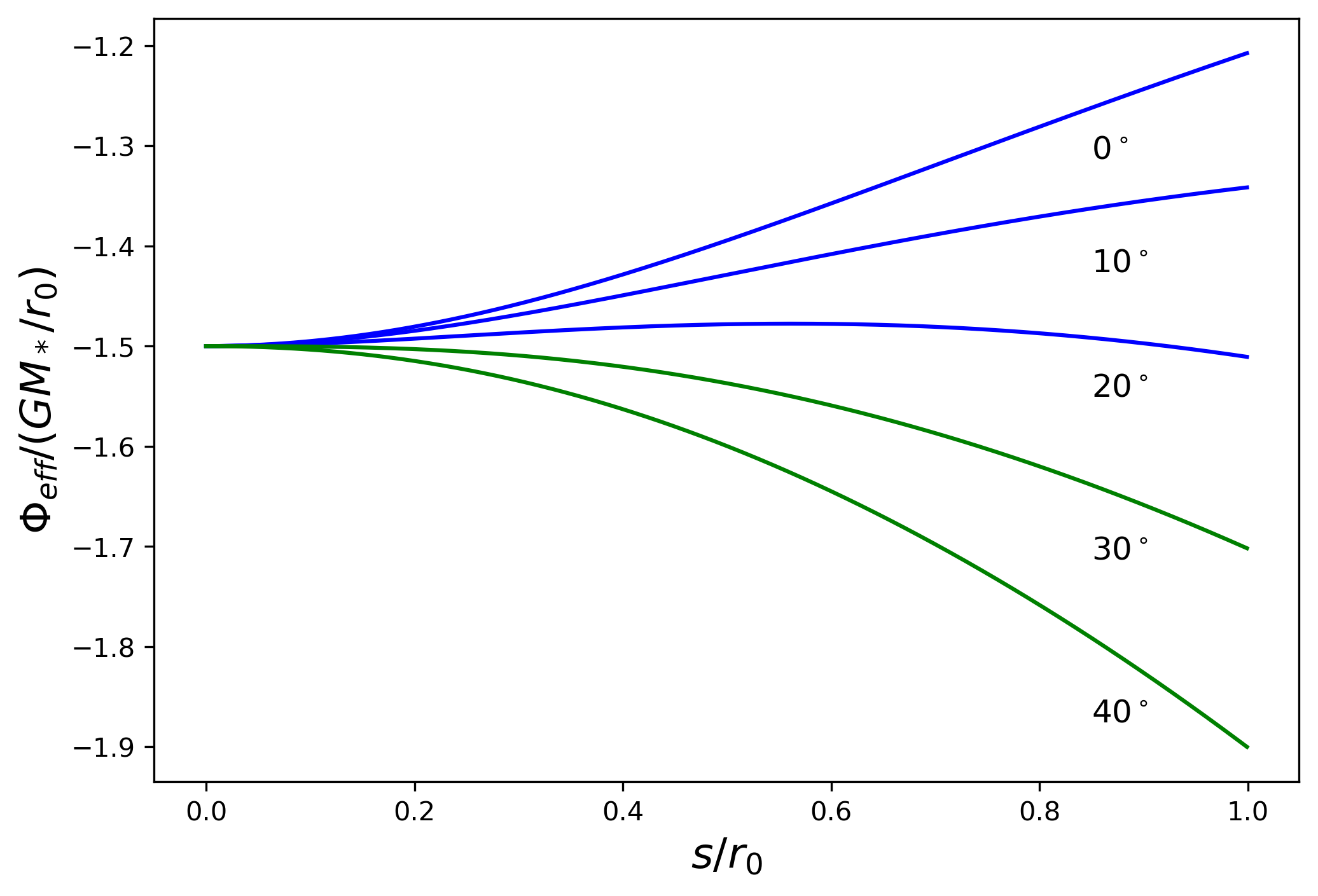
This function is plotted in Figure 9 for various values of the angle $\theta$. If we consider first a vertical field line ($\theta=0$) the effective potential is a monotonically increasing function of distance $s$. For modest values of $\theta$ there is a potential barrier defined by a maximum at some $s=s_{\rm max}$, while for large enough $\theta$ the potential decreases monotonically from $s=0$. In this last case purely magneto-centrifugal forces suffice to accelerate a wind off the disk surface, even in the absence of any thermal effects. We compute the critical inclination angle $\theta_{\rm crit}$, defined as the minimum angle that allows magneto-centrifugal wind driving, via the condition,

$$\left.\frac{\partial^{2}\Phi_{\rm eff}}{\partial s^{2}}\right|_{s=0}=0.$$

(87)

Evaluating this condition, we find,

	$\displaystyle 1-4\sin^{2}\theta_{\rm crit}$	$\displaystyle=$	$\displaystyle 0$
	$\displaystyle\Rightarrow\theta_{\rm crit}$	$\displaystyle=$	$\displaystyle 30^{\circ},$		(88)

as the minimum inclination angle from the vertical needed for unimpeded wind launching in ideal MHD.

The rigid rotation of the field lines interior to the Alfvén surface means that gas being accelerated along them increases its specific angular momentum. The magnetic field, in turn, applies a torque to the disk that removes a corresponding amount of angular momentum. If a field line, anchored to the disk at radius $r_{0}$, crosses the Alfvén surface at (cylindrical) radius $r_{A}$, it follows that the angular momentum flux is,

$$\dot{L}_{w}=\dot{M}_{w}\Omega_{0}r_{A}^{2},$$

(89)

where $\dot{M}_{w}$ is the mass loss rate in the wind. Removing angular momentum at this rate from the disk results in a local accretion rate $\dot{M}=2\dot{L}_{w}/\Omega_{0}r_{0}^{2}$. The ratio of the disk accretion rate to the wind loss rate is,

$$\frac{\dot{M}}{\dot{M}_{w}}=2\left(\frac{r_{A}}{r_{0}}\right)^{2}.$$

(90)

If $r_{A}$ substantially exceeds $r_{0}$ (by a factor of a few, which is reasonable for detailed disk wind solutions) a relatively weak wind can carry away enough angular momentum to support a much larger accretion rate.

In cylindrical polar co-ordinates $(r,\phi,z)$ the continuity equation is,

$$\frac{\partial\rho}{\partial t}+\frac{1}{r}\frac{\partial}{\partial r}\left(r\rho v_{r}\right)+\frac{1}{r}\frac{\partial}{\partial\phi}\left(\rho v_{\phi}\right)+\frac{\partial}{\partial z}\left(\rho v_{z}\right)=0.$$

(93)

Integrating over $\phi$ $[0,2\pi]$ and over $z$ $[-\infty,\infty]$ the first term becomes,

$$\frac{\partial}{\partial t}\int_{0}^{2\pi}\int_{-\infty}^{\infty}\rho dzd\phi=\frac{\partial}{\partial t}\left(2\pi\Sigma\right),$$

(94)

where $\Sigma(r,t)$ is the azimuthally averaged surface density. We are working toward an evolution equation for this quantity. Integrating the second term,

$$\frac{1}{r}\frac{\partial}{\partial r}\int_{0}^{2\pi}\int_{-\infty}^{\infty}r\rho v_{r}dzd\phi=\frac{1}{r}\frac{\partial{\cal{F}}}{\partial r},$$

(95)

where $\cal{F}$, the radial mass flux,

$${\cal{F}}=\int_{0}^{2\pi}\int_{-\infty}^{\infty}r\rho v_{r}dzd\phi=2\pi r\Sigma\bar{v}_{r},$$

(96)

can be written in terms of the surface density and the density-weighted radial velocity $\bar{v}_{r}$. On integration, the third and fourth terms vanish (the latter assuming that there is no mass loss from the surfaces of the disk) leaving,

$$\frac{\partial\Sigma}{\partial t}+\frac{1}{r}\frac{\partial}{\partial r}\left(r\Sigma\bar{v}_{r}\right)=0,$$

(97)

as the one-dimensional version of the continuity equation.

Dealing with the momentum equation in the same way, we can simplify the algebra by assuming at the outset that the disk is axisymmetric such that the orbital velocity,

$$v_{\phi}=r\Omega,$$

(98)

depends only on the angular velocity $\Omega=\Omega(r)$ of circular orbits in a fixed gravitational potential $\Phi$. The only non-zero terms in the $\phi$ component of the momentum equation then come from ${\bf v}\cdot\nabla{\bf v}$ and $\nabla{\bf\cdot T}$. Looking up the forms for these in cylindrical polar co-ordinates the surviving terms are,

	$\displaystyle\left.{\bf v}\cdot{\nabla{\bf v}}\right|_{\phi}$	$\displaystyle=$	$\displaystyle v_{r}\frac{\rm dv_{\phi}}{\rm dr}+\frac{v_{\phi}v_{r}}{r},$		(99)
	$\displaystyle\left.\frac{1}{\rho}\nabla\cdot{\bf T}\right|_{\phi}$	$\displaystyle=$	$\displaystyle\frac{1}{r^{2}\rho}\frac{\partial}{\partial r}\left(r^{2}T_{r\phi}\right)+\frac{1}{\rho}\frac{\partial T_{\phi z}}{\partial z}.$		(100)

Multiplying these expressions through by $r\rho$ the azimuthal component of the momentum equation takes the form,

$$\rho v_{r}\frac{{\rm d}h}{{\rm d}r}=\frac{1}{r}\frac{\partial}{\partial r}\left(r^{2}T_{r\phi}\right)+r\frac{\partial T_{\phi z}}{\partial z},$$

(101)

where the specific angular momentum $h$ is defined as,

$$h\equiv r^{2}\Omega.$$

(102)

Finally we multiply equation (101) through again by $r$, and integrate over $\phi$ and $z$. If $T_{\phi z}$ vanishes as $z\rightarrow\pm\infty$ the result is,

$${\cal{F}}\frac{{\rm d}h}{{\rm d}r}=-\frac{\partial{\cal G}}{\partial r},$$

(103)

where ${\cal F}$ is given by equation (96) and,

$${\cal{G}}=-\int_{0}^{2\pi}\int_{-\infty}^{\infty}r^{2}T_{r\phi}dzd\phi,$$

(104)

is the viscous torque.

Getting to this point from the conservation laws expressed in equation (92) requires only some rather transparent assumptions: axisymmetry, a time-independent potential, and no mass or angular momentum loss from the disk surfaces. One could stop there, and consider $T_{r\phi}$ to be the key quantity whose dependence on disk conditions needs to be determined. Conventionally, however, we instead write the torque in terms of an effective fluid viscosity that follows a Navier-Stokes form. For a fluid with viscosity $\mu$ and bulk viscosity $\mu_{\rm b}$ we have,

$${\bf T}=\mu\left[\nabla{\bf v}+\left(\nabla{\bf v}\right)^{T}\right]+\left(\mu_{\rm b}-\frac{2}{3}\mu\right)\left(\nabla\cdot{\bf v}\right){\bf I}.$$

(105)

To leading order the divergence of a thin disk velocity field vanishes, so we don’t have to worry about bulk viscosity at all. The $r\phi$ component of the stress is,

$$T_{r\phi}=\mu r\frac{{\rm d}\Omega}{{\rm d}r}.$$

(106)

Defining the kinematic viscosity (later just “the viscosity”) $\nu$ as,

$$\nu=\frac{1}{2\pi\Sigma}\int_{0}^{2\pi}\int_{-\infty}^{\infty}\mu dzd\phi,$$

(107)

the viscous torque has a fairly intuitive form that is the product of the circumference, the viscous force per unit length, and the lever arm,

$${\cal G}=-2\pi r\cdot\nu\Sigma r\frac{{\rm d}\Omega}{{\rm d}r}\cdot r.$$

(108)

Equation (103) is then,

$$\Sigma\bar{v}_{r}\frac{{\rm d}h}{{\rm d}r}=\frac{1}{r}\frac{\rm d}{{\rm d}r}\left(\nu\Sigma r^{3}\frac{{\rm d}\Omega}{{\rm d}r}\right).$$

(109)

Given the aforementioned assumptions, this equation expresses angular momentum conservation for a viscous fluid in a disk geometry.

Eliminating the radial velocity $\bar{v}_{r}$ between equation (97) and equation (109) we obtain,

$$\frac{\partial\Sigma}{\partial t}=-\frac{1}{r}\frac{\partial}{\partial r}\left[\left(\frac{{\rm d}h}{{\rm d}r}\right)^{-1}\frac{\partial}{\partial r}\left(\nu\Sigma r^{3}\frac{{\rm d}\Omega}{{\rm d}r}\right)\right].$$

(110)

This form is valid for an arbitrary (fixed) profile of angular velocity and angular momentum in the disk. Very often we are interested in the case of a disk that orbits a Newtonian point mass $M$. In that limit,

	$\displaystyle\Omega$	$\displaystyle=$	$\displaystyle\Omega_{\rm K}=\sqrt{GM/r^{3}},$		(111)
	$\displaystyle h$	$\displaystyle=$	$\displaystyle\sqrt{GMr}.$		(112)

The radial velocity is given by equation (109) as,

$$\bar{v}_{r}=-\frac{3}{\Sigma r^{1/2}}\frac{\rm d}{{\rm d}r}\left(\nu\Sigma r^{1/2}\right),$$

(113)

and the evolution equation has the form,

$$\frac{\partial\Sigma}{\partial t}=\frac{3}{r}\frac{\partial}{\partial r}\left[r^{1/2}\frac{\partial}{\partial r}\left(\nu\Sigma r^{1/2}\right)\right].$$

(114)

The surface density thus evolves according to a diffusive partial differential equation, whose precise character depends upon the nature of the viscosity. The equation is linear if $\nu\neq f(\Sigma)$, though there is no general reason for this to be the case.

Steady solutions to equation (114) are easily derived. Setting $\partial\Sigma/\partial t=0$ and integrating we find that,

$$\nu\Sigma=c_{1}+c_{2}r^{-1/2}.$$

(115)

Determining the constants of integration takes a little more work, and the right answer depends on the physics of the disk being modeled. It’s easiest to start from equation (109). Noting that the accretion rate $\dot{M}$ is,

$$\dot{M}=-2\pi r\Sigma\bar{v}_{r},$$

(116)

and that $\dot{M}$ must be constant for a steady solution, we integrate equation (109). The result is,

$$-\frac{\dot{M}}{2\pi}h=\nu\Sigma r^{3}\frac{{\rm d}\Omega}{{\rm d}r}+{\rm const}.$$

(117)

For Keplerian (point mass) forms for $h$ and $\Omega$, the constant term is negligible at large $r$. We have, as $r\rightarrow\infty$,

$$\nu\Sigma\simeq\frac{\dot{M}}{3\pi}.$$

(118)

The surface density of the disk is inversely proportional to the viscosity.

References

- Abramowicz et al. (1988) Abramowicz, M A, B. Czerny, J. P. Lasota, and E. Szuszkiewicz (1988), “Slim Accretion Disks,” Astrophys. J. 332, 646.
- Abramowicz and Fragile (2013) Abramowicz, Marek A, and P. Chris Fragile (2013), “Foundations of Black Hole Accretion Disk Theory,” Living Reviews in Relativity 16 (1), 1, arXiv:1104.5499 [astro-ph.HE] .
- Agol et al. (2001) Agol, Eric, Julian Krolik, Neal J. Turner, and James M. Stone (2001), “Two-dimensional Hydrodynamic Simulations of Convection in Radiation-dominated Accretion Disks,” Astrophys. J. 558 (2), 543–552, arXiv:astro-ph/0105137 [astro-ph] .
- Agol and Krolik (2000) Agol, Eric, and Julian H. Krolik (2000), “Magnetic Stress at the Marginally Stable Orbit: Altered Disk Structure, Radiation, and Black Hole Spin Evolution,” Astrophys. J. 528 (1), 161–170, arXiv:astro-ph/9908049 [astro-ph] .
- Alexander et al. (2014) Alexander, R, I. Pascucci, S. Andrews, P. Armitage, and L. Cieza (2014), “The Dispersal of Protoplanetary Disks,” in Protostars and Planets VI, edited by Henrik Beuther, Ralf S. Klessen, Cornelis P. Dullemond, and Thomas Henning, p. 475, arXiv:1311.1819 [astro-ph.EP] .
- Armitage (1998) Armitage, Philip J (1998), “Turbulence and Angular Momentum Transport in a Global Accretion Disk Simulation,” Astrophys. J. Lett. 501 (2), L189–L192, arXiv:astro-ph/9805133 [astro-ph] .
- Armitage et al. (2001) Armitage, Philip J, Mario Livio, and J. E. Pringle (2001), “Episodic accretion in magnetically layered protoplanetary discs,” MNRAS 324 (3), 705–711, arXiv:astro-ph/0101253 [astro-ph] .
- Audard et al. (2014) Audard, M, P. Ábrahám, M. M. Dunham, J. D. Green, N. Grosso, K. Hamaguchi, J. H. Kastner, Á. Kóspál, G. Lodato, M. M. Romanova, S. L. Skinner, E. I. Vorobyov, and Z. Zhu (2014), “Episodic Accretion in Young Stars,” in Protostars and Planets VI, edited by Henrik Beuther, Ralf S. Klessen, Cornelis P. Dullemond, and Thomas Henning, p. 387, arXiv:1401.3368 [astro-ph.SR] .
- Bai and Stone (2013) Bai, Xue-Ning, and James M. Stone (2013), “Local Study of Accretion Disks with a Strong Vertical Magnetic Field: Magnetorotational Instability and Disk Outflow,” Astrophys. J. 767 (1), 30, arXiv:1210.6661 [astro-ph.HE] .
- Balbus (2003) Balbus, Steven A (2003), “Enhanced Angular Momentum Transport in Accretion Disks,” ARA&A 41, 555–597, arXiv:astro-ph/0306208 [astro-ph] .
- Balbus (2017) Balbus, Steven A (2017), “The general relativistic thin disc evolution equation,” MNRAS 471 (4), 4832–4838, arXiv:1707.08884 [astro-ph.HE] .
- Balbus and Hawley (1991) Balbus, Steven A, and John F. Hawley (1991), “A Powerful Local Shear Instability in Weakly Magnetized Disks. I. Linear Analysis,” Astrophys. J. 376, 214.
- Balbus and Hawley (1992) Balbus, Steven A, and John F. Hawley (1992), “Is the Oort A-Value a Universal Growth Rate Limit for Accretion Disk Shear Instabilities?” Astrophys. J. 392, 662.
- Balbus and Hawley (1998) Balbus, Steven A, and John F. Hawley (1998), “Instability, turbulence, and enhanced transport in accretion disks,” Reviews of Modern Physics 70 (1), 1–53.
- Balbus and Henri (2008) Balbus, Steven A, and Pierre Henri (2008), “On the Magnetic Prandtl Number Behavior of Accretion Disks,” Astrophys. J. 674 (1), 408–414, arXiv:0706.0828 [astro-ph] .
- Bally and Scoville (1982) Bally, J, and N. Z. Scoville (1982), “Structure and evolution of molecular clouds near H II regions. II. The disk constrained H II region, S 106.” Astrophys. J. 255, 497–509.
- Bardeen (1970) Bardeen, James M (1970), “Kerr Metric Black Holes,” Nature (London) 226 (5240), 64–65.
- Bardeen and Petterson (1975) Bardeen, James M, and Jacobus A. Petterson (1975), “The Lense-Thirring Effect and Accretion Disks around Kerr Black Holes,” Astrophys. J. Lett. 195, L65.
- Bardeen et al. (1972) Bardeen, James M, William H. Press, and Saul A. Teukolsky (1972), “Rotating Black Holes: Locally Nonrotating Frames, Energy Extraction, and Scalar Synchrotron Radiation,” Astrophys. J. 178, 347–370.
- Bate et al. (2002) Bate, M R, G. I. Ogilvie, S. H. Lubow, and J. E. Pringle (2002), “The excitation, propagation and dissipation of waves in accretion discs: the non-linear axisymmetric case,” MNRAS 332 (3), 575–600, arXiv:astro-ph/0201149 [astro-ph] .
- Bath and Pringle (1982) Bath, G T, and J. E. Pringle (1982), “The evolution of viscous discs. II - Viscous variations,” MNRAS 199, 267–280.
- Begelman (1978) Begelman, M C (1978), “Black holes in radiation-dominated gas: an analogue of the Bondi accretion problem.” MNRAS 184, 53–67.
- Begelman et al. (1983) Begelman, M C, C. F. McKee, and G. A. Shields (1983), “Compton heated winds and coronae above accretion disks. I. Dynamics.” Astrophys. J. 271, 70–88.
- Begelman and Meier (1982) Begelman, M C, and D. L. Meier (1982), “Thick accretion disks - Self-similar, supercritical models,” Astrophys. J. 253, 873–896.
- Begelman and Pringle (2007) Begelman, M C, and J. E. Pringle (2007), “Accretion discs with strong toroidal magnetic fields,” MNRAS 375 (3), 1070–1076, arXiv:astro-ph/0612300 [astro-ph] .
- Begelman and Chiueh (1988) Begelman, Mitchell C, and Tzihong Chiueh (1988), “Thermal Coupling of Ions and Electrons by Collective Effects in Two-Temperature Accretion Flows,” Astrophys. J. 332, 872.
- Begelman et al. (2022) Begelman, Mitchell C, Nicolas Scepi, and Jason Dexter (2022), “What really makes an accretion disc MAD,” MNRAS 10.1093/mnras/stab3790, arXiv:2111.02439 [astro-ph.HE] .
- Begelman et al. (2006) Begelman, Mitchell C, Marta Volonteri, and Martin J. Rees (2006), “Formation of supermassive black holes by direct collapse in pre-galactic haloes,” MNRAS 370 (1), 289–298, arXiv:astro-ph/0602363 [astro-ph] .
- Bell and Lin (1994) Bell, K R, and D. N. C. Lin (1994), “Using FU Orionis Outbursts to Constrain Self-regulated Protostellar Disk Models,” Astrophys. J. 427, 987, arXiv:astro-ph/9312015 [astro-ph] .
- Blandford and Payne (1982) Blandford, R D, and D. G. Payne (1982), “Hydromagnetic flows from accretion disks and the production of radio jets.” MNRAS 199, 883–903.
- Blandford and Znajek (1977) Blandford, R D, and R. L. Znajek (1977), “Electromagnetic extraction of energy from Kerr black holes.” MNRAS 179, 433–456.
- Blandford and Begelman (1999) Blandford, Roger D, and Mitchell C. Begelman (1999), “On the fate of gas accreting at a low rate on to a black hole,” MNRAS 303 (1), L1–L5, arXiv:astro-ph/9809083 [astro-ph] .
- Blondin and Raymer (2012) Blondin, John M, and Eric Raymer (2012), “Hoyle-Lyttleton Accretion in Three Dimensions,” Astrophys. J. 752 (1), 30, arXiv:1204.0717 [astro-ph.SR] .
- Bollimpalli et al. (2018) Bollimpalli, D A, J. M. Hameury, and J. P. Lasota (2018), “Disc instabilities and nova eruptions in symbiotic systems: RS Ophiuchi and Z Andromedae,” MNRAS 481 (4), 5422–5435, arXiv:1804.07916 [astro-ph.HE] .
- Bondi (1952) Bondi, H (1952), “On spherically symmetrical accretion,” MNRAS 112, 195.
- Bondi and Hoyle (1944) Bondi, H, and F. Hoyle (1944), “On the mechanism of accretion by stars,” MNRAS 104, 273.
- Bonnerot et al. (2016) Bonnerot, Clément, Elena M. Rossi, Giuseppe Lodato, and Daniel J. Price (2016), “Disc formation from tidal disruptions of stars on eccentric orbits by Schwarzschild black holes,” MNRAS 455 (2), 2253–2266, arXiv:1501.04635 [astro-ph.HE] .
- Brandenburg et al. (1995) Brandenburg, Axel, Ake Nordlund, Robert F. Stein, and Ulf Torkelsson (1995), “Dynamo-generated Turbulence and Large-Scale Magnetic Fields in a Keplerian Shear Flow,” Astrophys. J. 446, 741.
- Cannizzo et al. (1982) Cannizzo, J K, P. Ghosh, and J. C. Wheeler (1982), “Convective accretion disks and the onset of dwarf nova outbursts.” Astrophys. J. Lett. 260, L83–L86.
- Cannizzo (1993) Cannizzo, John K (1993), “The Accretion Disk Limit Cycle Model: Toward an Understanding of the Long-Term Behavior of SS Cygni,” Astrophys. J. 419, 318.
- Cannizzo et al. (2012) Cannizzo, John K, Alan P. Smale, Matt A. Wood, Martin D. Still, and Steve B. Howell (2012), “The Kepler Light Curves of V1504 Cygni and V344 Lyrae: A Study of the Outburst Properties,” Astrophys. J. 747 (2), 117, arXiv:1112.4506 [astro-ph.SR] .
- Casassus et al. (2015) Casassus, S, S. Marino, S. Pérez, P. Roman, A. Dunhill, P. J. Armitage, J. Cuadra, A. Wootten, G. van der Plas, L. Cieza, Victor Moral, V. Christiaens, and Matías Montesinos (2015), “Accretion Kinematics through the Warped Transition Disk in HD142527 from Resolved CO(6-5) Observations,” Astrophys. J. 811 (2), 92, arXiv:1505.07732 [astro-ph.SR] .
- Castor et al. (1975) Castor, J I, D. C. Abbott, and R. I. Klein (1975), “Radiation-driven winds in Of stars.” Astrophys. J. 195, 157–174.
- Chan et al. (2018) Chan, Chi-Ho, Julian H. Krolik, and Tsvi Piran (2018), “Magnetorotational Instability in Eccentric Disks,” Astrophys. J. 856 (1), 12, arXiv:1712.01882 [astro-ph.HE] .
- Chandra et al. (2015) Chandra, Mani, Charles F. Gammie, Francois Foucart, and Eliot Quataert (2015), “An Extended Magnetohydrodynamics Model for Relativistic Weakly Collisional Plasmas,” Astrophys. J. 810 (2), 162, arXiv:1508.00878 [astro-ph.HE] .
- Chandrasekhar (1961) Chandrasekhar, Subrahmanyan (1961), Hydrodynamic and hydromagnetic stability.
- Chen and Beloborodov (2007) Chen, Wen-Xin, and Andrei M. Beloborodov (2007), “Neutrino-cooled Accretion Disks around Spinning Black Holes,” Astrophys. J. 657 (1), 383–399, arXiv:astro-ph/0607145 [astro-ph] .
- Chiang and Goldreich (1997) Chiang, E I, and P. Goldreich (1997), “Spectral Energy Distributions of T Tauri Stars with Passive Circumstellar Disks,” Astrophys. J. 490 (1), 368–376, arXiv:astro-ph/9706042 [astro-ph] .
- Clarke and Carswell (2007) Clarke, Cathie, and Bob Carswell (2007), Principles of Astrophysical Fluid Dynamics.
- Coleman et al. (2016) Coleman, M S B, I. Kotko, O. Blaes, J. P. Lasota, and S. Hirose (2016), “Dwarf nova outbursts with magnetorotational turbulence,” MNRAS 462 (4), 3710–3726, arXiv:1608.01321 [astro-ph.HE] .
- Coleman et al. (2018) Coleman, Matthew S B, Omer Blaes, Shigenobu Hirose, and Peter H. Hauschildt (2018), “Convection Enhances Magnetic Turbulence in AM CVn Accretion Disks,” Astrophys. J. 857 (1), 52, arXiv:1803.04381 [astro-ph.SR] .
- Cunningham (1976) Cunningham, C (1976), “Returning radiation in accretion disks around black holes.” Astrophys. J. 208, 534–549.
- D’Alessio et al. (1999) D’Alessio, Paola, Jorge Cantó, Lee Hartmann, Nuria Calvet, and Susana Lizano (1999), “On the Thermal Stability of Irradiation-dominated Pre-Main-Sequence Disks,” Astrophys. J. 511 (2), 896–903.
- Das et al. (2018) Das, Upasana, Mitchell C. Begelman, and Geoffroy Lesur (2018), “Instability in strongly magnetized accretion discs: a global perspective,” MNRAS 473 (2), 2791–2812, arXiv:1709.09173 [astro-ph.HE] .
- Davies and Pringle (1980) Davies, R E, and J. E. Pringle (1980), “On accretion from an inhomogeneous medium,” MNRAS 191, 599–604.
- Davis et al. (2010) Davis, Shane W, James M. Stone, and Martin E. Pessah (2010), “Sustained Magnetorotational Turbulence in Local Simulations of Stratified Disks with Zero Net Magnetic Flux,” Astrophys. J. 713 (1), 52–65, arXiv:0909.1570 [astro-ph.HE] .
- Davis and Tchekhovskoy (2020) Davis, Shane W, and Alexander Tchekhovskoy (2020), “Magnetohydrodynamics Simulations of Active Galactic Nucleus Disks and Jets,” ARA&A 58, 407–439, arXiv:2101.08839 [astro-ph.HE] .
- Demianski and Ivanov (1997) Demianski, M, and P. B. Ivanov (1997), “The dynamics of twisted accretion disc around a Kerr black hole.” A&A 324, 829–834.
- Deng et al. (2021) Deng, Hongping, Gordon I. Ogilvie, and Lucio Mayer (2021), “Parametric instability in a free-evolving warped protoplanetary disc,” MNRAS 500 (3), 4248–4256, arXiv:2010.00862 [astro-ph.EP] .
- Di Matteo et al. (2002) Di Matteo, Tiziana, Rosalba Perna, and Ramesh Narayan (2002), “Neutrino Trapping and Accretion Models for Gamma-Ray Bursts,” Astrophys. J. 579 (2), 706–715, arXiv:astro-ph/0207319 [astro-ph] .
- Doǧan et al. (2018) Doǧan, S, C. J. Nixon, A. R. King, and J. E. Pringle (2018), “Instability of warped discs,” MNRAS 476 (2), 1519–1531, arXiv:1801.05426 [astro-ph.HE] .
- Dubus et al. (1999) Dubus, Guillaume, Jean-Pierre Lasota, Jean-Marie Hameury, and Phil Charles (1999), “X-ray irradiation in low-mass binary systems,” MNRAS 303 (1), 139–147, arXiv:astro-ph/9809036 [astro-ph] .
- Dullemond (2000) Dullemond, C P (2000), “Are passive protostellar disks stable to self-shadowing?” A&A 361, L17–L20, arXiv:astro-ph/0007399 [astro-ph] .
- Dullemond et al. (2021) Dullemond, C P, C. N. Kimmig, and J. J. Zanazzi (2021), “On the equations of warped disc dynamics,” arXiv e-prints , arXiv:2109.12035arXiv:2109.12035 [astro-ph.SR] .
- Edgar (2004) Edgar, Richard (2004), “A review of Bondi-Hoyle-Lyttleton accretion,” New Astron. Rev. 48 (10), 843–859, arXiv:astro-ph/0406166 [astro-ph] .
- Ercolano and Pascucci (2017) Ercolano, Barbara, and Ilaria Pascucci (2017), “The dispersal of planet-forming discs: theory confronts observations,” Royal Society Open Science 4 (4), 170114, arXiv:1704.00214 [astro-ph.EP] .
- Event Horizon Telescope Collaboration et al. (2019) Event Horizon Telescope Collaboration,, Kazunori Akiyama, and et al. (2019), “First M87 Event Horizon Telescope Results. I. The Shadow of the Supermassive Black Hole,” Astrophys. J. Lett. 875 (1), L1, arXiv:1906.11238 [astro-ph.GA] .
- Faulkner et al. (1983) Faulkner, J, D. N. C. Lin, and J. Papaloizou (1983), “On the evolution of accretion disc flow in cataclysmic variables- I.The prospect of a limit cycle in dwarf nova systems.” MNRAS 205, 359–375.
- Fishbone and Moncrief (1976) Fishbone, L G, and V. Moncrief (1976), “Relativistic fluid disks in orbit around Kerr black holes.” Astrophys. J. 207, 962–976.
- Flaherty et al. (2020) Flaherty, Kevin, A. Meredith Hughes, Jacob B. Simon, Chunhua Qi, Xue-Ning Bai, Alyssa Bulatek, Sean M. Andrews, David J. Wilner, and Ágnes Kóspál (2020), “Measuring Turbulent Motion in Planet-forming Disks with ALMA: A Detection around DM Tau and Nondetections around MWC 480 and V4046 Sgr,” Astrophys. J. 895 (2), 109, arXiv:2004.12176 [astro-ph.SR] .
- Flaherty et al. (2017) Flaherty, Kevin M, A. Meredith Hughes, Sanaea C. Rose, Jacob B. Simon, Chunhua Qi, Sean M. Andrews, Ágnes Kóspál, David J. Wilner, Eugene Chiang, Philip J. Armitage, and Xue-ning Bai (2017), “A Three-dimensional View of Turbulence: Constraints on Turbulent Motions in the HD 163296 Protoplanetary Disk Using DCO+,” Astrophys. J. 843 (2), 150, arXiv:1706.04504 [astro-ph.EP] .
- Frank et al. (2002) Frank, Juhan, Andrew King, and Derek J. Raine (2002), Accretion Power in Astrophysics: Third Edition.
- Fromang (2013) Fromang, S (2013), “MRI-driven angular momentum transport in protoplanetary disks,” in EAS Publications Series, EAS Publications Series, Vol. 62, edited by P. Hennebelle and C. Charbonnel, pp. 95–142, arXiv:1305.3416 [astro-ph.SR] .
- Fromang et al. (2007) Fromang, S, J. Papaloizou, G. Lesur, and T. Heinemann (2007), “MHD simulations of the magnetorotational instability in a shearing box with zero net flux. II. The effect of transport coefficients,” A&A 476 (3), 1123–1132, arXiv:0705.3622 [astro-ph] .
- Gammie (1996) Gammie, Charles F (1996), “Layered Accretion in T Tauri Disks,” Astrophys. J. 457, 355.
- Gammie (1999a) Gammie, Charles F (1999a), “Efficiency of Magnetized Thin Accretion Disks in the Kerr Metric,” Astrophys. J. Lett. 522 (1), L57–L60, arXiv:astro-ph/9906223 [astro-ph] .
- Gammie (1999b) Gammie, Charles F (1999b), “Instabilities in Circumstellar Discs,” in Astrophysical Discs - an EC Summer School, Astronomical Society of the Pacific Conference Series, Vol. 160, edited by J. A. Sellwood and Jeremy Goodman, p. 122.
- Gammie (2001) Gammie, Charles F (2001), “Nonlinear Outcome of Gravitational Instability in Cooling, Gaseous Disks,” Astrophys. J. 553 (1), 174–183, arXiv:astro-ph/0101501 [astro-ph] .
- Gammie et al. (2000) Gammie, Charles F, Jeremy Goodman, and Gordon I. Ogilvie (2000), “Linear and non-linear theory of a parametric instability of hydrodynamic warps in Keplerian discs,” MNRAS 318 (4), 1005–1016, arXiv:astro-ph/0001539 [astro-ph] .
- Gerosa et al. (2020) Gerosa, Davide, Giovanni Rosotti, and Riccardo Barbieri (2020), “The Bardeen-Petterson effect in accreting supermassive black hole binaries: a systematic approach,” MNRAS 496 (3), 3060–3075, arXiv:2004.02894 [astro-ph.GA] .
- Goldreich and Lynden-Bell (1965) Goldreich, P, and D. Lynden-Bell (1965), “II. Spiral arms as sheared gravitational instabilities,” MNRAS 130, 125.
- Goldreich and Tremaine (1979) Goldreich, P, and S. Tremaine (1979), “The excitation of density waves at the Lindblad and corotation resonances by an external potential.” Astrophys. J. 233, 857–871.
- Goodchild and Ogilvie (2006) Goodchild, Simon, and Gordon Ogilvie (2006), “The dynamics of eccentric accretion discs in superhump systems,” MNRAS 368 (3), 1123–1131, arXiv:astro-ph/0602492 [astro-ph] .
- Goodman (2003) Goodman, Jeremy (2003), “Self-gravity and quasi-stellar object discs,” MNRAS 339 (4), 937–948, arXiv:astro-ph/0201001 [astro-ph] .
- Gruzinov (1998) Gruzinov, Andrei V (1998), “Radiative Efficiency of Collisionless Accretion,” Astrophys. J. 501 (2), 787–791, arXiv:astro-ph/9710132 [astro-ph] .
- Hameury (2020) Hameury, J M (2020), “A review of the disc instability model for dwarf novae, soft X-ray transients and related objects,” Advances in Space Research 66 (5), 1004–1024, arXiv:1910.01852 [astro-ph.SR] .
- Harris et al. (2020) Harris, Charles R, K. Jarrod Millman, St’efan J. van der Walt, Ralf Gommers, Pauli Virtanen, David Cournapeau, Eric Wieser, Julian Taylor, Sebastian Berg, Nathaniel J. Smith, Robert Kern, Matti Picus, Stephan Hoyer, Marten H. van Kerkwijk, Matthew Brett, Allan Haldane, Jaime Fern’andez del R’ıo, Mark Wiebe, Pearu Peterson, Pierre G’erard-Marchant, Kevin Sheppard, Tyler Reddy, Warren Weckesser, Hameer Abbasi, Christoph Gohlke, and Travis E. Oliphant (2020), “Array programming with NumPy,” Nature 585 (7825), 357–362.
- Hartmann et al. (1998) Hartmann, Lee, Nuria Calvet, Erik Gullbring, and Paola D’Alessio (1998), “Accretion and the Evolution of T Tauri Disks,” Astrophys. J. 495 (1), 385–400.
- Hawley et al. (1995) Hawley, John F, Charles F. Gammie, and Steven A. Balbus (1995), “Local Three-dimensional Magnetohydrodynamic Simulations of Accretion Disks,” Astrophys. J. 440, 742.
- Hill (1878) Hill, G W (1878), “Researches in the lunar theory,” American Journal of Mathematics 1 (1), 5–26.
- Hirose et al. (2014) Hirose, Shigenobu, Omer Blaes, Julian H. Krolik, Matthew S. B. Coleman, and Takayoshi Sano (2014), “Convection Causes Enhanced Magnetic Turbulence in Accretion Disks in Outburst,” Astrophys. J. 787 (1), 1, arXiv:1403.3096 [astro-ph.HE] .
- Hirose et al. (2009) Hirose, Shigenobu, Julian H. Krolik, and Omer Blaes (2009), “Radiation-Dominated Disks are Thermally Stable,” Astrophys. J. 691 (1), 16–31, arXiv:0809.1708 [astro-ph] .
- Hōshi (1979) Hōshi, R (1979), “Accretion Model for Outbursts of Dwarf Nova,” Progress of Theoretical Physics 61 (5), 1307–1319.
- Hoyle and Lyttleton (1939) Hoyle, F, and R. A. Lyttleton (1939), “The effect of interstellar matter on climatic variation,” Proceedings of the Cambridge Philosophical Society 35 (3), 405.
- Hughes et al. (2011) Hughes, A Meredith, David J. Wilner, Sean M. Andrews, Chunhua Qi, and Michiel R. Hogerheijde (2011), “Empirical Constraints on Turbulence in Protoplanetary Accretion Disks,” Astrophys. J. 727 (2), 85, arXiv:1011.3826 [astro-ph.SR] .
- Hunter (2007) Hunter, J D (2007), “Matplotlib: A 2d graphics environment,” Computing in Science & Engineering 9 (3), 90–95.
- Ichimaru (1977) Ichimaru, S (1977), “Bimodal behavior of accretion disks: theory and application to Cygnus X-1 transitions.” Astrophys. J. 214, 840–855.
- Igumenshchev (2008) Igumenshchev, Igor V (2008), “Magnetically Arrested Disks and the Origin of Poynting Jets: A Numerical Study,” Astrophys. J. 677 (1), 317–326, arXiv:0711.4391 [astro-ph] .
- Jiang et al. (2019a) Jiang, Yan-Fei, Omer Blaes, James M. Stone, and Shane W. Davis (2019a), “Global Radiation Magnetohydrodynamic Simulations of sub-Eddington Accretion Disks around Supermassive Black Holes,” Astrophys. J. 885 (2), 144, arXiv:1904.01674 [astro-ph.HE] .
- Jiang et al. (2013) Jiang, Yan-Fei, James M. Stone, and Shane W. Davis (2013), “On the Thermal Stability of Radiation-dominated Accretion Disks,” Astrophys. J. 778 (1), 65, arXiv:1309.5646 [astro-ph.HE] .
- Jiang et al. (2019b) Jiang, Yan-Fei, James M. Stone, and Shane W. Davis (2019b), “Super-Eddington Accretion Disks around Supermassive Black Holes,” Astrophys. J. 880 (2), 67, arXiv:1709.02845 [astro-ph.HE] .
- Kato (1983) Kato, S (1983), “Low-frequency, one-armed oscillations of Keplerian gaseous disks.” PASJ 35, 249–261.
- Kato (2016) Kato, Shoji (2016), Oscillations of Disks, Vol. 437.
- Katz (1973) Katz, J I (1973), “Thirty-five-day Periodicity in Her X-1,” Nature Physical Science 246 (154), 87–89.
- Kenyon and Hartmann (1987) Kenyon, S J, and L. Hartmann (1987), “Spectral Energy Distributions of T Tauri Stars: Disk Flaring and Limits on Accretion,” Astrophys. J. 323, 714.
- Kerr (1963) Kerr, Roy P (1963), “Gravitational Field of a Spinning Mass as an Example of Algebraically Special Metrics,” Phys. Rev. Lett. 11 (5), 237–238.
- King et al. (2005) King, A R, S. H. Lubow, G. I. Ogilvie, and J. E. Pringle (2005), “Aligning spinning black holes and accretion discs,” MNRAS 363 (1), 49–56, arXiv:astro-ph/0507098 [astro-ph] .
- King and Pringle (2006) King, A R, and J. E. Pringle (2006), “Growing supermassive black holes by chaotic accretion,” MNRAS 373 (1), L90–L92, arXiv:astro-ph/0609598 [astro-ph] .
- King et al. (2007) King, A R, J. E. Pringle, and M. Livio (2007), “Accretion disc viscosity: how big is alpha?” MNRAS 376 (4), 1740–1746, arXiv:astro-ph/0701803 [astro-ph] .
- Kluyver et al. (2016) Kluyver, Thomas, Benjamin Ragan-Kelley, Fernando Pérez, Brian Granger, Matthias Bussonnier, Jonathan Frederic, Kyle Kelley, Jessica Hamrick, Jason Grout, Sylvain Corlay, Paul Ivanov, Damián Avila, Safia Abdalla, Carol Willing, and Jupyter development team (2016), “Jupyter notebooks - a publishing format for reproducible computational workflows,” in Positioning and Power in Academic Publishing: Players, Agents and Agendas, edited by Fernando Loizides and Birgit Scmidt (IOS Press, Netherlands) pp. 87–90.
- Kozai (1962) Kozai, Yoshihide (1962), “Secular perturbations of asteroids with high inclination and eccentricity,” AJ 67, 591–598.
- Kratter and Lodato (2016) Kratter, Kaitlin, and Giuseppe Lodato (2016), “Gravitational Instabilities in Circumstellar Disks,” ARA&A 54, 271–311, arXiv:1603.01280 [astro-ph.SR] .
- Kratter et al. (2010) Kratter, Kaitlin M, Christopher D. Matzner, Mark R. Krumholz, and Richard I. Klein (2010), “On the Role of Disks in the Formation of Stellar Systems: A Numerical Parameter Study of Rapid Accretion,” Astrophys. J. 708 (2), 1585–1597, arXiv:0907.3476 [astro-ph.SR] .
- Kraus et al. (2020) Kraus, Stefan, Alexander Kreplin, Alison K. Young, Matthew R. Bate, John D. Monnier, Tim J. Harries, Henning Avenhaus, Jacques Kluska, Anna S. E. Laws, Evan A. Rich, Matthew Willson, Alicia N. Aarnio, Fred C. Adams, Sean M. Andrews, Narsireddy Anugu, Jaehan Bae, Theo ten Brummelaar, Nuria Calvet, Michel Curé, Claire L. Davies, Jacob Ennis, Catherine Espaillat, Tyler Gardner, Lee Hartmann, Sasha Hinkley, Aaron Labdon, Cyprien Lanthermann, Jean-Baptiste LeBouquin, Gail H. Schaefer, Benjamin R. Setterholm, David Wilner, and Zhaohuan Zhu (2020), “A triple-star system with a misaligned and warped circumstellar disk shaped by disk tearing,” Science 369 (6508), 1233–1238, arXiv:2004.01204 [astro-ph.SR] .
- Krolik and Zweibel (2006) Krolik, Julian H, and Ellen G. Zweibel (2006), “The Weak-Field Limit of the Magnetorotational Instability,” Astrophys. J. 644 (1), 651–661, arXiv:astro-ph/0602317 [astro-ph] .
- Krumholz et al. (2006) Krumholz, Mark R, Christopher F. McKee, and Richard I. Klein (2006), “Bondi-Hoyle Accretion in a Turbulent Medium,” Astrophys. J. 638 (1), 369–381, arXiv:astro-ph/0510410 [astro-ph] .
- Kumar and Pringle (1985) Kumar, S, and J. E. Pringle (1985), “Twisted accretion discs - The Bardeen-Petterson effect,” MNRAS 213, 435–442.
- Lai (2003) Lai, Dong (2003), “Warping of Accretion Disks with Magnetically Driven Outflows: A Possible Origin for Jet Precession,” Astrophys. J. Lett. 591 (2), L119–L122, arXiv:astro-ph/0306012 [astro-ph] .
- Lasota (2001) Lasota, Jean-Pierre (2001), “The disc instability model of dwarf novae and low-mass X-ray binary transients,” New Astron. Rev. 45 (7), 449–508, arXiv:astro-ph/0102072 [astro-ph] .
- Latter et al. (2015) Latter, Henrik N, Sebastien Fromang, and Julien Faure (2015), “Local and global aspects of the linear MRI in accretion discs,” MNRAS 453 (3), 3257–3268, arXiv:1508.03012 [astro-ph.HE] .
- Latter and Papaloizou (2017) Latter, Henrik N, and John Papaloizou (2017), “Local models of astrophysical discs,” MNRAS 472 (2), 1432–1446, arXiv:1708.09285 [astro-ph.HE] .
- Lee and Goodman (1999) Lee, Erick, and Jeremy Goodman (1999), “Non-linear single-armed spiral density waves in nearly Keplerian discs,” MNRAS 308 (4), 984–994, arXiv:astro-ph/9905197 [astro-ph] .
- Lense and Thirring (1918) Lense, Josef, and Hans Thirring (1918), “Über den Einfluß der Eigenrotation der Zentralkörper auf die Bewegung der Planeten und Monde nach der Einsteinschen Gravitationstheorie,” Physikalische Zeitschrift 19, 156.
- Levin (2007) Levin, Yuri (2007), “Starbursts near supermassive black holes: young stars in the Galactic Centre, and gravitational waves in LISA band,” MNRAS 374 (2), 515–524, arXiv:astro-ph/0603583 [astro-ph] .
- Li et al. (2001) Li, H, S. A. Colgate, B. Wendroff, and R. Liska (2001), “Rossby Wave Instability of Thin Accretion Disks. III. Nonlinear Simulations,” Astrophys. J. 551 (2), 874–896, arXiv:astro-ph/0012479 [astro-ph] .
- Lidov (1962) Lidov, M L (1962), “The evolution of orbits of artificial satellites of planets under the action of gravitational perturbations of external bodies,” Planetary and Space Science 9 (10), 719–759.
- Lightman and Eardley (1974) Lightman, Alan P, and Douglas M. Eardley (1974), “Black Holes in Binary Systems: Instability of Disk Accretion,” Astrophys. J. Lett. 187, L1.
- Lin et al. (1990) Lin, D N C, J. C. B. Papaloizou, and G. J. Savonije (1990), “Propagation of Tidal Disturbance in Gaseous Accretion Disks,” Astrophys. J. 365, 748.
- Liska et al. (2021) Liska, M, C. Hesp, A. Tchekhovskoy, A. Ingram, M. van der Klis, S. B. Markoff, and M. Van Moer (2021), “Disc tearing and Bardeen-Petterson alignment in GRMHD simulations of highly tilted thin accretion discs,” MNRAS 507 (1), 983–990, arXiv:1904.08428 [astro-ph.HE] .
- Livio et al. (1986) Livio, M, N. Soker, M. de Kool, and G. J. Savonije (1986), “Accretion from an inhomogeneous medium - III. General case and observational consequences.” MNRAS 222, 235–250.
- Lodato and Pringle (2007) Lodato, Giuseppe, and J. E. Pringle (2007), “Warp diffusion in accretion discs: a numerical investigation,” MNRAS 381 (3), 1287–1300, arXiv:0708.1124 [astro-ph] .
- Lovelace and Hohlfeld (1978) Lovelace, R V E, and R. G. Hohlfeld (1978), “Negative mass instability of flat galaxies.” Astrophys. J. 221, 51–61.
- Lovelace et al. (1999) Lovelace, R V E, H. Li, S. A. Colgate, and A. F. Nelson (1999), “Rossby Wave Instability of Keplerian Accretion Disks,” Astrophys. J. 513 (2), 805–810, arXiv:astro-ph/9809321 [astro-ph] .
- Lubow and Ogilvie (2000) Lubow, S H, and G. I. Ogilvie (2000), “On the Tilting of Protostellar Disks by Resonant Tidal Effects,” Astrophys. J. 538 (1), 326–340, arXiv:astro-ph/0003028 [astro-ph] .
- Lubow et al. (1994) Lubow, S H, J. C. B. Papaloizou, and J. E. Pringle (1994), “Magnetic field dragging in accretion discs,” MNRAS 267 (2), 235–240.
- Lubow and Ogilvie (2017) Lubow, Stephen H, and Gordon I. Ogilvie (2017), “Kozai-Lidov disc instability,” MNRAS 469 (4), 4292–4305, arXiv:1704.07522 [astro-ph.SR] .
- Lynch and Ogilvie (2021a) Lynch, Elliot M, and Gordon I. Ogilvie (2021a), “Dynamical structure of highly eccentric discs with applications to tidal disruption events,” MNRAS 500 (3), 4110–4125, arXiv:2011.02219 [astro-ph.HE] .
- Lynch and Ogilvie (2021b) Lynch, Elliot M, and Gordon I. Ogilvie (2021b), “Importance of magnetic fields in highly eccentric discs with applications to tidal disruption events,” MNRAS 501 (4), 5500–5516, arXiv:2101.01221 [astro-ph.HE] .
- Lynden-Bell (1996) Lynden-Bell, D (1996), “Magnetic collimation by accretion discs of quasars and stars,” MNRAS 279 (2), 389–401.
- Lynden-Bell and Pringle (1974) Lynden-Bell, D, and J. E. Pringle (1974), “The evolution of viscous discs and the origin of the nebular variables.” MNRAS 168, 603–637.
- Lyra and Umurhan (2019) Lyra, Wladimir, and Orkan M. Umurhan (2019), “The Initial Conditions for Planet Formation: Turbulence Driven by Hydrodynamical Instabilities in Disks around Young Stars,” PASP 131 (1001), 072001, arXiv:1808.08681 [astro-ph.EP] .
- Lyubarskij et al. (1994) Lyubarskij, Y E, K. A. Postnov, and M. E. Prokhorov (1994), “Eccentric Accretion Discs,” MNRAS 266, 583.
- MacFadyen and Woosley (1999) MacFadyen, A I, and S. E. Woosley (1999), “Collapsars: Gamma-Ray Bursts and Explosions in “Failed Supernovae”,” Astrophys. J. 524 (1), 262–289, arXiv:astro-ph/9810274 [astro-ph] .
- MacLeod and Ramirez-Ruiz (2015) MacLeod, Morgan, and Enrico Ramirez-Ruiz (2015), “Asymmetric Accretion Flows within a Common Envelope,” Astrophys. J. 803 (1), 41, arXiv:1410.3823 [astro-ph.SR] .
- Mahadevan and Quataert (1997) Mahadevan, Rohan, and Eliot Quataert (1997), “Are Particles in Advection-dominated Accretion Flows Thermal?” Astrophys. J. 490 (2), 605–618, arXiv:astro-ph/9705067 [astro-ph] .
- Maloney et al. (1996) Maloney, Philip R, Mitchell C. Begelman, and J. E. Pringle (1996), “Radiation-driven Warping: The Origin of WARPS and Precession in Accretion Disks,” Astrophys. J. 472, 582, arXiv:astro-ph/9612110 [astro-ph] .
- Marrone et al. (2007) Marrone, Daniel P, James M. Moran, Jun-Hui Zhao, and Ramprasad Rao (2007), “An Unambiguous Detection of Faraday Rotation in Sagittarius A*,” Astrophys. J. Lett. 654 (1), L57–L60, arXiv:astro-ph/0611791 [astro-ph] .
- Martin and Lubow (2011) Martin, R G, and S. H. Lubow (2011), “The Gravo-magneto Limit Cycle in Accretion Disks,” Astrophys. J. Lett. 740 (1), L6, arXiv:1108.4960 [astro-ph.SR] .
- Martin et al. (2019) Martin, Rebecca G, Stephen H. Lubow, J. E. Pringle, Alessia Franchini, Zhaohuan Zhu, Stephen Lepp, Rebecca Nealon, C. J. Nixon, and David Vallet (2019), “Generalized Warped Disk Equations,” Astrophys. J. 875 (1), 5, arXiv:1902.11073 [astro-ph.HE] .
- Martin et al. (2014) Martin, Rebecca G, Chris Nixon, Stephen H. Lubow, Philip J. Armitage, Daniel J. Price, Suzan Doğan, and Andrew King (2014), “The Kozai-Lidov Mechanism in Hydrodynamical Disks,” Astrophys. J. Lett. 792 (2), L33, arXiv:1409.1226 [astro-ph.EP] .
- Martin et al. (2007) Martin, Rebecca G, J. E. Pringle, and Christopher A. Tout (2007), “Alignment and precession of a black hole with a warped accretion disc,” MNRAS 381 (4), 1617–1624, arXiv:0708.2034 [astro-ph] .
- Matsuda et al. (1991) Matsuda, T, N. Sekino, K. Sawada, E. Shima, M. Livio, U. Anzer, and G. Boerner (1991), “On the stability of wind accretion.” A&A 248, 301.
- McNally and Pessah (2015) McNally, Colin P, and Martin E. Pessah (2015), “On Vertically Global, Horizontally Local Models for Astrophysical Disks,” Astrophys. J. 811 (2), 121, arXiv:1406.4864 [astro-ph.EP] .
- Meyer and Meyer-Hofmeister (1981) Meyer, F, and E. Meyer-Hofmeister (1981), “On the elusive cause of cataclysmic variable outbursts.” A&A 104, L10–L12.
- Mineshige and Osaki (1983a) Mineshige, S, and Y. Osaki (1983a), “Disk-instability model for outbursts of dwarf novae Time-dependent formulation and one-zone model,” PASJ 35 (3), 377–396.
- Mineshige and Osaki (1983b) Mineshige, S, and Y. Osaki (1983b), “Disk-instability model for outbursts of dwarf novae Time-dependent formulation and one-zone model,” PASJ 35 (3), 377–396.
- Mishra et al. (2016) Mishra, B, P. C. Fragile, L. C. Johnson, and W. Kluźniak (2016), “Three-dimensional, global, radiative GRMHD simulations of a thermally unstable disc,” MNRAS 463 (4), 3437–3448, arXiv:1603.04082 [astro-ph.HE] .
- Mishra et al. (2020) Mishra, Bhupendra, Mitchell C. Begelman, Philip J. Armitage, and Jacob B. Simon (2020), “Strongly magnetized accretion discs: structure and accretion from global magnetohydrodynamic simulations,” MNRAS 492 (2), 1855–1868, arXiv:1907.08995 [astro-ph.HE] .
- Miyoshi et al. (1995) Miyoshi, Makoto, James Moran, James Herrnstein, Lincoln Greenhill, Naomasa Nakai, Philip Diamond, and Makoto Inoue (1995), “Evidence for a black hole from high rotation velocities in a sub-parsec region of NGC4258,” Nature (London) 373 (6510), 127–129.
- Mortlock et al. (2011) Mortlock, Daniel J, Stephen J. Warren, Bram P. Venemans, Mitesh Patel, Paul C. Hewett, Richard G. McMahon, Chris Simpson, Tom Theuns, Eduardo A. Gonzáles-Solares, Andy Adamson, Simon Dye, Nigel C. Hambly, Paul Hirst, Mike J. Irwin, Ernst Kuiper, Andy Lawrence, and Huub J. A. Röttgering (2011), “A luminous quasar at a redshift of z = 7.085,” Nature (London) 474 (7353), 616–619, arXiv:1106.6088 [astro-ph.CO] .
- Naoz (2016) Naoz, Smadar (2016), “The Eccentric Kozai-Lidov Effect and Its Applications,” ARA&A 54, 441–489, arXiv:1601.07175 [astro-ph.EP] .
- Narayan et al. (2000) Narayan, Ramesh, Igor V. Igumenshchev, and Marek A. Abramowicz (2000), “Self-similar Accretion Flows with Convection,” Astrophys. J. 539 (2), 798–808, arXiv:astro-ph/9912449 [astro-ph] .
- Narayan and Yi (1994) Narayan, Ramesh, and Insu Yi (1994), “Advection-dominated Accretion: A Self-similar Solution,” Astrophys. J. Lett. 428, L13, arXiv:astro-ph/9403052 [astro-ph] .
- Narayan and Yi (1995a) Narayan, Ramesh, and Insu Yi (1995a), “Advection-dominated Accretion: Self-Similarity and Bipolar Outflows,” Astrophys. J. 444, 231, arXiv:astro-ph/9411058 [astro-ph] .
- Narayan and Yi (1995b) Narayan, Ramesh, and Insu Yi (1995b), “Advection-dominated Accretion: Underfed Black Holes and Neutron Stars,” Astrophys. J. 452, 710, arXiv:astro-ph/9411059 [astro-ph] .
- Natarajan and Armitage (1999) Natarajan, Priyamvada, and Philip J. Armitage (1999), “Warped discs and the directional stability of jets in active galactic nuclei,” MNRAS 309 (4), 961–968, arXiv:astro-ph/9812001 [astro-ph] .
- Natarajan and Pringle (1998) Natarajan, Priyamvada, and J. E. Pringle (1998), “The Alignment of Disk and Black Hole Spins in Active Galactic Nuclei,” Astrophys. J. Lett. 506 (2), L97–L100, arXiv:astro-ph/9808187 [astro-ph] .
- Nixon and Pringle (2020) Nixon, C J, and J. E. Pringle (2020), “Accretion discs with non-zero central torque,” arXiv e-prints , arXiv:2008.07565arXiv:2008.07565 [astro-ph.HE] .
- Nixon and King (2016) Nixon, Chris, and Andrew King (2016), “Warp Propagation in Astrophysical Discs,” in Lecture Notes in Physics, Berlin Springer Verlag, Vol. 905, edited by Francesco Haardt, Vittorio Gorini, Ugo Moschella, Aldo Treves, and Monica Colpi, p. 45.
- Nixon et al. (2013) Nixon, Chris, Andrew King, and Daniel Price (2013), “Tearing up the disc: misaligned accretion on to a binary,” MNRAS 434 (3), 1946–1954, arXiv:1307.0010 [astro-ph.HE] .
- Nixon et al. (2012) Nixon, Chris, Andrew King, Daniel Price, and Juhan Frank (2012), “Tearing up the Disk: How Black Holes Accrete,” Astrophys. J. Lett. 757 (2), L24, arXiv:1209.1393 [astro-ph.HE] .
- Nixon and King (2012) Nixon, Christopher J, and Andrew R. King (2012), “Broken discs: warp propagation in accretion discs,” MNRAS 421 (2), 1201–1208, arXiv:1201.1297 [astro-ph.HE] .
- Novikov and Thorne (1973) Novikov, I D, and K. S. Thorne (1973), “Astrophysics of black holes.” in Black Holes (Les Astres Occlus), pp. 343–450.
- Oda et al. (2009) Oda, H, M. Machida, K. E. Nakamura, and R. Matsumoto (2009), “Thermal Equilibria of Magnetically Supported Black Hole Accretion Disks,” Astrophys. J. 697 (1), 16–28, arXiv:0903.0477 [astro-ph.HE] .
- Ogilvie (1999a) Ogilvie, G I (1999a), “The non-linear fluid dynamics of a warped accretion disc,” MNRAS 304 (3), 557–578, arXiv:astro-ph/9812073 [astro-ph] .
- Ogilvie (1999b) Ogilvie, G I (1999b), “Time-dependent quasi-spherical accretion,” MNRAS 306 (1), L9–L13, arXiv:astro-ph/9905089 [astro-ph] .
- Ogilvie (2001) Ogilvie, G I (2001), “Non-linear fluid dynamics of eccentric discs,” MNRAS 325 (1), 231–248, arXiv:astro-ph/0102245 [astro-ph] .
- Ogilvie (2006) Ogilvie, G I (2006), “Non-linear bending waves in Keplerian accretion discs,” MNRAS 365 (3), 977–990, arXiv:astro-ph/0510681 [astro-ph] .
- Ogilvie and Barker (2014) Ogilvie, Gordon I, and Adrian J. Barker (2014), “Local and global dynamics of eccentric astrophysical discs,” MNRAS 445 (3), 2621–2636, arXiv:1409.6487 [astro-ph.EP] .
- Ogilvie and Latter (2013) Ogilvie, Gordon I, and Henrik N. Latter (2013), “Local and global dynamics of warped astrophysical discs,” MNRAS 433 (3), 2403–2419, arXiv:1303.0263 [astro-ph.SR] .
- Osaki (1974) Osaki, Y (1974), “An Accretion Model for the Outbursts of U Geminorum Stars,” PASJ 26, 429.
- Oyang et al. (2021) Oyang, Bryance, Yan-Fei Jiang, and Omer Blaes (2021), “Investigating lack of accretion disc eccentricity growth in a global 3D MHD simulation of a superhump system,” MNRAS 505 (1), 1–17, arXiv:2105.02392 [astro-ph.HE] .
- Paczynski (1978) Paczynski, B (1978), “A model of selfgravitating accretion disk.” Acta Astron. 28, 91–109.
- Page and Thorne (1974) Page, Don N, and Kip S. Thorne (1974), “Disk-Accretion onto a Black Hole. Time-Averaged Structure of Accretion Disk,” Astrophys. J. 191, 499–506.
- Papaloizou (2002) Papaloizou, J C B (2002), “Global m = 1 modes and migration of protoplanetary cores in eccentric protoplanetary discs,” A&A 388, 615–631, arXiv:astro-ph/0204197 [astro-ph] .
- Papaloizou (2005) Papaloizou, J C B (2005), “The local instability of steady astrophysical flows with non circular streamlines with application to differentially rotating disks with free eccentricity,” A&A 432 (3), 743–755, arXiv:astro-ph/0412587 [astro-ph] .
- Papaloizou and Lin (1995) Papaloizou, J C B, and D. N. C. Lin (1995), “On the Dynamics of Warped Accretion Disks,” Astrophys. J. 438, 841.
- Papaloizou and Pringle (1983) Papaloizou, J C B, and J. E. Pringle (1983), “The time-dependence of non-planar accretion discs,” MNRAS 202, 1181–1194.
- Papaloizou and Terquem (1995) Papaloizou, John C B, and Caroline Terquem (1995), “On the dynamics of tilted discs around young stars,” MNRAS 274 (4), 987–1001.
- Paris and Ogilvie (2018) Paris, J B, and G. I. Ogilvie (2018), “A local model of warped magnetized accretion discs,” MNRAS 477 (2), 2406–2418, arXiv:1803.00543 [astro-ph.SR] .
- Parker (1958) Parker, E N (1958), “Dynamics of the Interplanetary Gas and Magnetic Fields.” Astrophys. J. 128, 664.
- Pessah and Psaltis (2005) Pessah, Martin E, and Dimitrios Psaltis (2005), “The Stability of Magnetized Rotating Plasmas with Superthermal Fields,” Astrophys. J. 628 (2), 879–901, arXiv:astro-ph/0406071 [astro-ph] .
- Pierens et al. (2020) Pierens, Arnaud, Colin P. McNally, and Richard P. Nelson (2020), “Hydrodynamical turbulence in eccentric circumbinary discs and its impact on the in situ formation of circumbinary planets,” MNRAS 496 (3), 2849–2867, arXiv:2005.14693 [astro-ph.EP] .
- Popham et al. (1999) Popham, Robert, S. E. Woosley, and Chris Fryer (1999), “Hyperaccreting Black Holes and Gamma-Ray Bursts,” Astrophys. J. 518 (1), 356–374, arXiv:astro-ph/9807028 [astro-ph] .
- Potter and Balbus (2014) Potter, William J, and Steven A. Balbus (2014), “An accretion disc instability induced by a temperature sensitive parameter,” MNRAS 441 (1), 681–689, arXiv:1404.0013 [astro-ph.HE] .
- Pringle (1977) Pringle, J E (1977), “Soft X-ray emission from dwarf novae.” MNRAS 178, 195–202.
- Pringle (1981) Pringle, J E (1981), “Accretion discs in astrophysics,” ARA&A 19, 137–162.
- Pringle (1991) Pringle, J E (1991), “The properties of external accretion discs.” MNRAS 248, 754.
- Pringle (1992) Pringle, J E (1992), “A simple approach to the evolution of twisted accretion discs,” MNRAS 258 (4), 811–818.
- Pringle (1996) Pringle, J E (1996), “Self-induced warping of accretion discs,” MNRAS 281 (1), 357–361.
- Pringle and King (2007) Pringle, James E, and Andrew King (2007), Astrophysical Flows.
- Proga et al. (2000) Proga, Daniel, James M. Stone, and Timothy R. Kallman (2000), “Dynamics of Line-driven Disk Winds in Active Galactic Nuclei,” Astrophys. J. 543 (2), 686–696, arXiv:astro-ph/0005315 [astro-ph] .
- Quataert (1998) Quataert, Eliot (1998), “Particle Heating by Alfvénic Turbulence in Hot Accretion Flows,” Astrophys. J. 500 (2), 978–991, arXiv:astro-ph/9710127 [astro-ph] .
- Quataert and Gruzinov (2000) Quataert, Eliot, and Andrei Gruzinov (2000), “Convection-dominated Accretion Flows,” Astrophys. J. 539 (2), 809–814, arXiv:astro-ph/9912440 [astro-ph] .
- Rafikov (2015) Rafikov, Roman R (2015), “Viscosity Prescription for Gravitationally Unstable Accretion Disks,” Astrophys. J. 804 (1), 62, arXiv:1501.04980 [astro-ph.EP] .
- Rafikov (2016) Rafikov, Roman R (2016), “Generalized Similarity for Accretion/Decretion Disks,” Astrophys. J. 830 (1), 7, arXiv:1604.07439 [astro-ph.SR] .
- Rees et al. (1982) Rees, M J, M. C. Begelman, R. D. Blandford, and E. S. Phinney (1982), “Ion-supported tori and the origin of radio jets,” Nature (London) 295 (5844), 17–21.
- Reynolds (2021) Reynolds, Christopher S (2021), “Observational Constraints on Black Hole Spin,” ARA&A 59, 10.1146/annurev-astro-112420-035022, arXiv:2011.08948 [astro-ph.HE] .
- Rice et al. (2005) Rice, W K M, G. Lodato, and P. J. Armitage (2005), “Investigating fragmentation conditions in self-gravitating accretion discs,” MNRAS 364 (1), L56–L60, arXiv:astro-ph/0509413 [astro-ph] .
- Richard et al. (2013) Richard, S, P. Barge, and S. Le Dizès (2013), “Structure, stability, and evolution of 3D Rossby vortices in protoplanetary disks,” A&A 559, A30, arXiv:1309.3486 [astro-ph.EP] .
- Ruffert (1999) Ruffert, M (1999), “Non-axisymmetric wind-accretion simulations. II. Density gradients,” A&A 346, 861–877, arXiv:astro-ph/9903304 [astro-ph] .
- Ryan et al. (2017) Ryan, Benjamin R, Charles F. Gammie, Sebastien Fromang, and Pierre Kestener (2017), “Resolution Dependence of Magnetorotational Turbulence in the Isothermal Stratified Shearing Box,” Astrophys. J. 840 (1), 6, arXiv:1702.00777 [astro-ph.HE] .
- Rybicki and Lightman (1979) Rybicki, George B, and Alan P. Lightman (1979), Radiative processes in astrophysics.
- Ryu et al. (2021) Ryu, Taeho, Julian Krolik, and Tsvi Piran (2021), “The Impact of Shocks on the Vertical Structure of Eccentric Disks,” arXiv e-prints , arXiv:2105.09434arXiv:2105.09434 [astro-ph.HE] .
- Sadowski (2016) Sadowski, Aleksander (2016), “Thin accretion discs are stabilized by a strong magnetic field,” MNRAS 459 (4), 4397–4407, arXiv:1601.06785 [astro-ph.HE] .
- Safronov (1972) Safronov, V S (1972), Evolution of the protoplanetary cloud and formation of the earth and planets.
- Salpeter (1964) Salpeter, E E (1964), “Accretion of Interstellar Matter by Massive Objects.” Astrophys. J. 140, 796–800.
- Salvesen et al. (2016) Salvesen, Greg, Jacob B. Simon, Philip J. Armitage, and Mitchell C. Begelman (2016), “Accretion disc dynamo activity in local simulations spanning weak-to-strong net vertical magnetic flux regimes,” MNRAS 457 (1), 857–874, arXiv:1511.06368 [astro-ph.HE] .
- Scepi et al. (2018) Scepi, N, G. Lesur, G. Dubus, and M. Flock (2018), “Impact of convection and resistivity on angular momentum transport in dwarf novae,” A&A 609, A77, arXiv:1710.05872 [astro-ph.SR] .
- Scepi et al. (2019) Scepi, Nicolas, Guillaume Dubus, and Geoffroy Lesur (2019), “Magnetic wind-driven accretion in dwarf novae,” A&A 626, A116, arXiv:1812.02076 [astro-ph.HE] .
- Schandl and Meyer (1994) Schandl, S, and F. Meyer (1994), “Herculis X-1: coronal winds producing the tilted shape of the accretion disk.” A&A 289, 149–161.
- Schekochihin et al. (2019) Schekochihin, A A, Y. Kawazura, and M. A. Barnes (2019), “Constraints on ion versus electron heating by plasma turbulence at low beta,” Journal of Plasma Physics 85 (3), 905850303, arXiv:1812.09792 [physics.plasm-ph] .
- Schekochihin et al. (2004) Schekochihin, Alexander A, Steven C. Cowley, Samuel F. Taylor, Jason L. Maron, and James C. McWilliams (2004), “Simulations of the Small-Scale Turbulent Dynamo,” Astrophys. J. 612 (1), 276–307, arXiv:astro-ph/0312046 [astro-ph] .
- Scheuer and Feiler (1996) Scheuer, P A G, and R. Feiler (1996), “The realignment of a black hole misaligned with its accretion disc,” MNRAS 282, 291.
- Shakura and Sunyaev (1973) Shakura, N I, and R. A. Sunyaev (1973), “Reprint of 1973A&A….24..337S. Black holes in binary systems. Observational appearance.” A&A 500, 33–51.
- Shakura and Sunyaev (1976) Shakura, N I, and R. A. Sunyaev (1976), “A theory of the instability of disk accretion on to black holes and the variability of binary X-ray sources, galactic nuclei and quasars.” MNRAS 175, 613–632.
- Shapiro et al. (1976) Shapiro, S L, A. P. Lightman, and D. M. Eardley (1976), “A two-temperature accretion disk model for Cygnus X-1: structure and spectrum.” Astrophys. J. 204, 187–199.
- Shapiro and Teukolsky (1983) Shapiro, Stuart L, and Saul A. Teukolsky (1983), Black holes, white dwarfs, and neutron stars : the physics of compact objects.
- Shlosman et al. (1990) Shlosman, Isaac, Mitchell C. Begelman, and Julian Frank (1990), “The fuelling of active galactic nuclei,” Nature (London) 345 (6277), 679–686.
- Shu et al. (1994) Shu, Frank, Joan Najita, Eve Ostriker, Frank Wilkin, Steven Ruden, and Susana Lizano (1994), “Magnetocentrifugally Driven Flows from Young Stars and Disks. I. A Generalized Model,” Astrophys. J. 429, 781.
- Simon et al. (2012) Simon, Jacob B, Kris Beckwith, and Philip J. Armitage (2012), “Emergent mesoscale phenomena in magnetized accretion disc turbulence,” MNRAS 422 (3), 2685–2700, arXiv:1203.0314 [astro-ph.SR] .
- Sironi and Narayan (2015) Sironi, Lorenzo, and Ramesh Narayan (2015), “Electron Heating by the Ion Cyclotron Instability in Collisionless Accretion Flows. I. Compression-driven Instabilities and the Electron Heating Mechanism,” Astrophys. J. 800 (2), 88, arXiv:1411.5685 [astro-ph.HE] .
- Smak (1984) Smak, J (1984), “Accretion in cataclysmic binaries. IV. Accretion disks in dwarf novae.” Acta Astron. 34, 161–189.
- Soltan (1982) Soltan, A (1982), “Masses of quasars.” MNRAS 200, 115–122.
- Spitzer (1940) Spitzer, Lyman, Jr (1940), “The stability of isolated clusters,” MNRAS 100, 396.
- Spitzer (1962) Spitzer, L (1962), Physics of Fully Ionized Gases.
- Spruit (1996) Spruit, H C (1996), “Magnetohydrodynamic jets and winds from accretion disks,” in NATO Advanced Science Institutes (ASI) Series C, NATO Advanced Science Institutes (ASI) Series C, Vol. 477, edited by Ralph A. M. J. Wijers, Melvyn B. Davies, and Christopher A. Tout, pp. 249–286.
- Taam and Fryxell (1988) Taam, Ronald E, and B. A. Fryxell (1988), “On Nonsteady Accretion in Stellar Wind–fed X-Ray Sources,” Astrophys. J. Lett. 327, L73.
- Tabone et al. (2021) Tabone, Benoît, Giovanni P. Rosotti, Alexander J. Cridland, Philip J. Armitage, and Giuseppe Lodato (2021), “Secular evolution of MHD wind-driven discs: analytical solutions in the expanded -framework,” MNRAS 10.1093/mnras/stab3442, arXiv:2111.10145 [astro-ph.SR] .
- Tchekhovskoy et al. (2011) Tchekhovskoy, Alexander, Ramesh Narayan, and Jonathan C. McKinney (2011), “Efficient generation of jets from magnetically arrested accretion on a rapidly spinning black hole,” MNRAS 418 (1), L79–L83, arXiv:1108.0412 [astro-ph.HE] .
- Thorne (1974) Thorne, Kip S (1974), “Disk-Accretion onto a Black Hole. II. Evolution of the Hole,” Astrophys. J. 191, 507–520.
- Thorne and Blandford (2017) Thorne, Kip S, and Roger D. Blandford (2017), Modern Classical Physics: Optics, Fluids, Plasmas, Elasticity, Relativity, and Statistical Physics.
- Toomre (1964) Toomre, A (1964), “On the gravitational stability of a disk of stars.” Astrophys. J. 139, 1217–1238.
- Tremaine (2001) Tremaine, Scott (2001), “Slow Modes in Keplerian Disks,” AJ 121 (3), 1776–1789, arXiv:astro-ph/0011571 [astro-ph] .
- Ueda et al. (2021) Ueda, Takahiro, Mario Flock, and Tilman Birnstiel (2021), “Thermal Wave Instability as an Origin of Gap and Ring Structures in Protoplanetary Disks,” Astrophys. J. Lett. 914 (2), L38, arXiv:2105.13852 [astro-ph.EP] .
- Velikhov (1959) Velikhov, E P (1959), “Stability of an ideally conducting liquid flowing between rotating cylinders in a magnetic field,” Zhur. Eksptl’. i Teoret. Fiz. 36.
- Wang et al. (2021) Wang, Feige, Jinyi Yang, Xiaohui Fan, Joseph F. Hennawi, Aaron J. Barth, Eduardo Banados, Fuyan Bian, Konstantina Boutsia, Thomas Connor, Frederick B. Davies, Roberto Decarli, Anna-Christina Eilers, Emanuele Paolo Farina, Richard Green, Linhua Jiang, Jiang-Tao Li, Chiara Mazzucchelli, Riccardo Nanni, Jan-Torge Schindler, Bram Venemans, Fabian Walter, Xue-Bing Wu, and Minghao Yue (2021), “A Luminous Quasar at Redshift 7.642,” Astrophys. J. Lett. 907 (1), L1, arXiv:2101.03179 [astro-ph.GA] .
- Warner (1995) Warner, Brian (1995), Cataclysmic variable stars, Vol. 28.
- Watanabe and Lin (2008) Watanabe, Sei-ichiro, and D. N. C. Lin (2008), “Thermal Waves in Irradiated Protoplanetary Disks,” Astrophys. J. 672 (2), 1183–1195, arXiv:0709.1760 [astro-ph] .
- Whitehurst (1988) Whitehurst, Robert (1988), “Numerical simulations of accretion discs - I. Superhumps : a tidal phenomenon of accretion discs.” MNRAS 232, 35–51.
- Wienkers and Ogilvie (2018) Wienkers, A F, and G. I. Ogilvie (2018), “Non-linear hydrodynamic instability and turbulence in eccentric astrophysical discs with vertical structure,” MNRAS 477 (4), 4838–4855, arXiv:1804.03249 [astro-ph.EP] .
- Wijers and Pringle (1999) Wijers, Ralph A M J, and J. E. Pringle (1999), “Warped accretion discs and the long periods in X-ray binaries,” MNRAS 308 (1), 207–220, arXiv:astro-ph/9811056 [astro-ph] .
- Wu and Lithwick (2021) Wu, Yanqin, and Yoram Lithwick (2021), “The Irradiation Instability of Protoplanetary Disks,” Astrophys. J. 923 (1), 123, arXiv:2105.02680 [astro-ph.EP] .
- Xu and Stone (2019) Xu, Wenrui, and James M. Stone (2019), “Bondi-Hoyle-Lyttleton accretion in supergiant X-ray binaries: stability and disc formation,” MNRAS 488 (4), 5162–5184, arXiv:1907.06108 [astro-ph.HE] .
- Yu and Tremaine (2002) Yu, Qingjuan, and Scott Tremaine (2002), “Observational constraints on growth of massive black holes,” MNRAS 335 (4), 965–976, arXiv:astro-ph/0203082 [astro-ph] .
- Yuan and Narayan (2014) Yuan, Feng, and Ramesh Narayan (2014), “Hot Accretion Flows Around Black Holes,” ARA&A 52, 529–588, arXiv:1401.0586 [astro-ph.HE] .
- Zanazzi and Lai (2017) Zanazzi, J J, and Dong Lai (2017), “Lidov-Kozai Mechanism in Hydrodynamical Disks: Linear Stability Analysis,” MNRAS 467 (2), 1957–1964, arXiv:1612.05598 [astro-ph.EP] .
- Zanazzi and Ogilvie (2020) Zanazzi, J J, and Gordon I. Ogilvie (2020), “Eccentric tidal disruption event discs around supermassive black holes: dynamics and thermal emission,” MNRAS 499 (4), 5562–5577, arXiv:2009.06636 [astro-ph.HE] .
- Zhdankin et al. (2019) Zhdankin, Vladimir, Dmitri A. Uzdensky, Gregory R. Werner, and Mitchell C. Begelman (2019), “Electron and Ion Energization in Relativistic Plasma Turbulence,” Phys. Rev. Lett. 122 (5), 055101, arXiv:1809.01966 [astro-ph.HE] .
- Zhu et al. (2009) Zhu, Zhaohuan, Lee Hartmann, and Charles Gammie (2009), “Nonsteady Accretion in Protostars,” Astrophys. J. 694 (2), 1045–1055, arXiv:0811.1762 [astro-ph] .
- Zhu and Stone (2018) Zhu, Zhaohuan, and James M. Stone (2018), “Global Evolution of an Accretion Disk with a Net Vertical Field: Coronal Accretion, Flux Transport, and Disk Winds,” Astrophys. J. 857 (1), 34, arXiv:1701.04627 [astro-ph.EP] .