The influence of spatial configuration in collective transitions:
the importance of being sortedPreprint: APS/123-QED
Abstract
We studied the effects of spatial configuration on collective dynamics in a nearest-neighbour and diffusively coupled lattice of heterogeneous nodes. The networks contained nodes from two populations, which differed in their intrinsic excitability. Initially, these populations were uniformly and randomly distributed throughout the lattice. We then developed an iterative algorithm for perturbing the arrangement of the network such that nodes from the same population were increasingly likely to be adjacent to one another. We found that the global input strength, or network drive, necessary to transition the network from a state of quiescence to a state of synchronised and oscillatory activity was decreased as network sortedness was increased. Moreover, for weak coupling, we found that regimes of partial synchronisation exist (i.e. 2:1 resonance in the activity of the two populations), which were dependent both on network drive (sometimes in a non-monotonic fashion) and network sortedness.
Keywords:
Excitable systems, collective dynamics, beta cell, sortednessI Introduction
Many nonlinear systems exhibit excitable behaviour, whereby they exhibit large-amplitude oscillations in response to small-amplitude, transient perturbations. Such excitable dynamics are observed in semiconductor lasers Terrien et al. 2020; Terrien et al. 2021, social media networks Mathiesen et al. 2013, epidemiology Vannucchi and Boccaletti 2004, and wildfires Punckt et al. 2015. One prominent example is electrically excitable cells, such as neurons Izhikevich 2000; De Maesschalck and Wechselberger 2015; Wedgwood et al. 2021, cardiac cells Majumder et al. 2018; Barrio et al. 2020, pituitary cells Sanchez-Cardenas et al. 2010; Hodson et al. 2012 and pancreatic beta cells Bertram et al. 2007; McKenna et al. 2016. When excitable units are combined into networks, they can generate complex rhythms Bittihn et al. 2017; Hörning et al. 2017; Fretter et al. 2017. Interestingly, such networks may also generate dynamics that occur over low-dimensional manifolds of the full system Ashwin and Swift 1992; Watanabe and Strogatz 1993; Ott and Antonsen 2009; Bick et al. 2020. For example, neurons in the pre-Bötzinger complex fire synchronously to induce the inspiratory and expiratory phases during breathing Wittmeier et al. 2008; Gaiteri and Rubin 2011.
Heterogeneity is ubiquitous in natural systems. Whilst often portrayed as a undesirable attribute, it can play an important role in governing network dynamics Manchanda et al. 2017; Delgado et al. 2018; Lambert and Vanni 2018. For example, neurons may coarsely be stratified into excitatory and inhibitory groups, with the former promoting firing behaviour in other neurons and the latter suppressing it. When coupled, these neuronal subtypes give rise to a variety of behaviours, including synchronisation, and enable the network to respond differentially to incoming inputs Börgers and Kopell 2003; Börgers et al. 2005; Kopell et al. 2010. The classification of neuronal subtypes is becoming ever finer Gouwens et al. 2019; Lipovsek et al. 2021 and it remains an open question as to how this heterogeneity governs overall brain dynamics. Even when networks comprise only a single unit type, heterogeneity may still impact the global dynamics. For example, if the natural frequencies of nodes in a coupled oscillator network are too far apart, the network will be unable to synchronise and will instead display more complex rhythms Ottino-Löffler and Strogatz 2016.
Here, we explore transitions to synchrony in a locally-coupled network of heterogeneous, excitable nodes. As a motivating example, we consider networks of pancreatic beta cells. Individually, these cells exhibit excitable dynamics akin to the Hodgkin–Huxley model of nerve cells Hodgkin and Huxley 1952. Cells remain at rest until they receive a significantly large electrical impulse or the extracellular concentration of glucose surpasses a threshold value Ashcroft Frances M and Rorsman 1989; Braun et al. 2008. Under sustained suprathreshold stimulation, cells exhibit repetitive bursting-type dynamics comprising epochs of firing activity, followed by periods of rest Kinard et al. 1999. Beta cells are arranged into diffusively, and locally-coupled networks via channels known as gap junctions Rorsman and Braun 2013; Benninger et al. 2011. These networks exhibit synchronous bursting activity when exposed to sufficiently high levels of glucose Markovič et al. 2015. Although exogenous factors, such as incretin Hodson et al. 2014 and paracrine Caicedo 2013 signalling influence this coordinated beta cell response, the importance of intercellular coupling has been highlighted in several studies that demonstrate that synchronous beta cell rhythms are disrupted when gap junctions are blocked Head et al. 2012; Benninger and Piston 2014.
Based on empirical evidence from rodents, it has generally been assumed that beta cells form a syncticium, such that the activity of the network can be described by a single cell Dolenšek et al. 2013; Satin et al. 2020; Podobnik et al. 2020. Recent studies have challenged this perspective, highlighting that some ‘leader cells’ disproportionately influence the activity of a entire network made up primarily of ‘follower cells’ Johnston et al. 2016; Westacott et al. 2017; Salem et al. 2019; Benninger and Kravets 2021. One hypothesis suggests that islets are composed of a small number (10%) of highly excitable cells, with the remainder being less excitable Benninger and Hodson 2018. In this study, we explore how the spatial organisation of these two sub-populations affects the propensity of the whole network to oscillate in a synchronous fashion. The remainder of the manuscript is arranged as follows: In Sec. II, we describe the beta cell model, introduce a metric that captures how sorted a network is with respect to its heterogeneity, and present an algorithm that can generate networks with arbitrary sortedness. In Sec. III, we investigate how dynamic transitions to synchronous bursting depends of the degree of sortedness in the network and end in Sec. IV with concluding remarks.
II Methods
II.1 Mathematical model
We consider a network of diffusively-coupled excitable cells from a model describing electrical activity in pancreatic beta cells in the presence of glucose (Sherman et al. 1988). These cells exhibit bursting dynamics (in voltage ) when the glucose level, , is sufficiently high. The system possesses a slow variable, , representing Ca2+ concentration, which oscillates when the cell is active. We arrange nodes on a hexagonal close-packed (hcp) lattice embedded within a sphere. Each node is connected to its nearest neighbours via gap-junction coupling. The parameter sets the excitability of single cells within the network (Fig. S1). We define two sub-populations of nodes distinguished by their excitability. Population 1 is highly excitable () and population 2 is less excitable (). We then consider the range over where population 1 nodes are intrinsically active, while population 2 cells are intrinsically inactive. A full description of the mathematical model is provided in Sec. S1.1.
II.2 Measuring sortedness
To track the degree of sortedness in the network, we define a node sortedness measure that, for a given node, measures the proportion of neighbours that are of the same population type. For a general network with nodes attributed to populations, the node sortedness, , is defined as
| (1) |
where the population sets contain the indices of the nodes within population and form a partition over the node indices , is the set of indices of nodes that are adjacent to node , is an indicator function that takes value 1 if belongs to population and value 0 otherwise, and is an indicator function that takes value 1 when node and belong to the same population and value 0 otherwise. For each population, the average node sortedness is defined via
| (2) |
Finally, the network sortedness is defined as
| (3) |
where and, for the present case with , . For a network in which populations are assigned to nodes following a uniformly random distribution, since is approximately equal to where , is the number of nodes in population . and therefore . An illustration of the computation of the sortedness metrics (1)-(3) is shown in Fig. S8.
II.3 Modifying network sortedness
Here, we describe our approach for generating networks with different network sortednesss. The algorithm works by exchanging the population type of nodes from different populations randomly to increase (or decrease) . The algorithm begins by randomly permuting the order of the indices. The first indices of the permuted sequence are attributed to , with the remaining indices attributed to , yielding a distribution of population 1 nodes that is uniformly random in space.
On each iteration, , of the algorithm, pairs of nodes (from different populations) are sampled without replacement from a joint probability density function (pdf)
| (4) |
where and are random integer variables indicating the node selected from population 1 and 2, respectively. The population types of these nodes are then exchanged, that is, if and , then is added to and removed from and vice versa for . The network sortedness (3) is then recomputed for the adjusted population sets. If the exchange leads to an increase (decrease) in , the exchange is accepted and the algorithm proceeds to iteration . If the exchange does not lead to an increase (decrease) in , the exchange is rejected and indices and are placed back in and , respectively. In this case, a new pair of nodes is drawn from and the process is repeated until either: a pair whose exchange leads to an increase (decrease) in is found and the algorithm proceeds to the next iteration; or it is determined that no such pair exists, at which point the algorithm terminates. An example of one iteration of this algorithm is depicted in Fig. S9. We refer to the algorithm in which swaps are accepted only if they lead to an increase (decrease) in as the forward (backward) algorithm. We define to be the evaluation of of the network after iterations. Running the algorithm to convergence produces the sets containing the population sets after each iteration.
II.3.1 Modified sortedness metrics
Although the algorithm yields well-sorted networks with a small number of clusters of nodes from population 1, these clusters preferentially form at the edges of the domain. The average node sortedness, as defined in (2), for population 1 is maximised when a single cluster of population 1 nodes is coupled to the smallest possible number of population 2 nodes. This naturally occurs at the edges of the domain, since any cluster of population 1 nodes in the domain interior must be surrounded by population 2 nodes. We are interested in the dynamics that arise as the small population of highly excitable cells forms clusters within the lattice, hence, we wish to remove this tendency for clusters to form at the domain boundary. To overcome this, we use a modified definition of the node sortedness (1)
| (5) |
where is the number of connections that interior lattice nodes possess. For nodes with (i.e., nodes on the domain boundary) the additional term in (5) compared to (1) incorporates a further connections to population 2 nodes for the purposes of calculating node sortedness values. This procedure is equivalent to assuming that the lattice defining our domain is embedded within a larger lattice of population 2 nodes. An example of the computation of network sortedness using (5) is shown in Fig. 1. Pseudocode for the network sortedness manipulation algorithm is provided in Sec. S1.3.

II.3.2 Node selection probabilities
In this section, we formulate the node selection pdf used in the network sortedness adjustment algorithm. We assume that the selection of node from is independent of the selection of node from so that (4) becomes
| (6) |
One choice would set and to be uniform over and , respectively. Empirical observations of the algorithm outcome in this case demonstrate that clusters of population 1 nodes tend to form at the edge of the domain (not shown). As discussed in Sec. II.3.1, we wish to avoid this scenario. The tendency for clusters to form near the edge occurs because of the spherical nature of our lattice domain. In particular, a uniform choice for and means that nodes at the centre of the domain are less likely to be selected under a uniformly random sampling of indices than those at the edge because the number of nodes in the network increases superlinearly with respect to the domain radius. Therefore, we derive choices for that equalise the probability of a node being selected on the basis of its radial coordinate. The heuristic for generating will be the same as that for generating up to the population identity.
Denote the radial distance from the origin of node by where are the Cartesian coordinates of the location of the node. We define a sequences of intervals, , for with where so that each node is assigned to exactly one interval. The set of nodes from belonging to a given interval is given by . Using these set definitions, the pdf may be defined as
| (7) |
where is such that and is a normalisation factor ensuring that . This choice for reweights the probability of a given node being selected by a factor proportional to the number of cells from the same population within a spherical annulus with inner and outer radii specified by the boundaries of the intervals . This reweighting favours selecting nodes closer to the centre of the domain over those more distal.
II.4 Evaluation of collective dynamics
To characterise the network dynamics, we consider two features based on the Ca2+ trajectories across all nodes, namely, the mean number of peaks () and the time-averaged degree of synchronisation () calculated as the average magnitude of the Kuramoto order parameter (S13). The mean number of Ca2+ peaks across all nodes is proportional to the network participation, that is, the fraction of nodes that undergo oscillation. The value of captures the network coordination, tracking how closely the phases of the Ca2+ trajectories stay to one another across the simulation duration. We additionally define and where to be the mean number of peaks in Ca2+ and the time-averaged degree of synchronisation across nodes in population , respectively.
III Results
III.1 Simulating dynamics on the set of networks defined by running the swapping algorithm to convergence
We ran the swapping algorithm to convergence (in the forward direction and with 10% of the nodes specified to be from population 1) to produce sets and . For this run, the network configuration converged after iterations with a corresponding sortedness of the terminal network configuration of . We then simulated the dynamical system (S1)-(S11) for equispaced values of , as described in Sec. S1.2 for , and each configuration of populations defined by the population sets contained in and for . We ran each simulation for ms ( minutes), and discarded the initial 90,000 ms of resulting times series to control for transients. Each network configuration was simulated three times using each of a pre-defined set of initial conditions. Finally, we ran simulations once more using the first of these initial conditions to verify that results were consistent when the simulation duration was increased. We then calculated the features and for each simulation.
To aid in interpreting the results, we define the following sets. Firstly, the parameter domain over which we evaluated the dynamical system was . Secondly, the level sets , , and (for ) were used to delineate subsets of with qualitatively distinct network dynamics, which will be described below.
III.1.1 Increasing lowers the drive required for a transition to globally synchronised bursting when coupling is strong

We first sought to establish whether there is a relationship between and the level of drive required to activate the network. Shown in Fig. S10 is an example in which the transition from global quiescence to global activation is dependent on both and for the strongly coupled () case and where population 1 nodes comprise of the network. The mean of the Ca2+ trajectories for population 1 and 2 across the network are plotted for several values of and , which shows that as increases, the required drive to activate the network decreases. To examine trends across a range of network configurations, we plot the features (Fig. 2A, Fig. S11A), and (Fig. 2B, Fig. S11B) as a function of both and . Each point depicts a value , where , taken to be the median feature across the three simulations (which differ only in their initial condition). For strong coupling, we found that can be separated into a quiescent regime () and an oscillatory one (). The level set curve separating these regimes can be parameterised as a non-increasing function of (i.e., ), supporting the hypothesis that increasing decreases the drive required for network activation (Fig. 2A, B white curve). Similarly, the level set can be parameterised as a non-increasing function of that also separates the domains and (Fig. 2A, B black curve).
To investigate the robustness of the above relationships, we plotted and resulting from each of the three initial conditions (Fig. S12). We defined curves (Fig. S12, white curves) and (Fig. S12, black curves), in the same manner as described above. These curves are not identical across the choices of initial condition, and both curves are non-monotonic for the third initial condition, suggesting that multi-stability exists for some , at least near the transition between regimes and .
III.1.2 A domain with intra-population synchronicity and inter-population resonance exists when coupling is lowered to an intermediate strength

When (intermediate strength coupling), the threshold for activation of the network was lower than in the case of strong coupling, owing to the reduction of the suppressing effect of the less excitable population 2 nodes on the more excitable population 1 nodes. As in Sec. III.1.1, we plot the features (Fig. 3A, Fig. S13A) and (Fig. 3B, Fig. S13B) within the parameter domain , taking the median across three initial conditions We observed that the domain can be separated into three regimes with qualitatively distinct dynamics. The first two regimes, and , contain dynamics where the majority of nodes are quiescent or active (Fig. 3A) and synchronised (Fig. 3B), respectively. Within the third regime, denoted , we found high intra-population synchronisation, with population 2 nodes oscillating (w.r.t. Ca2+) at a frequency approximately half that of the population 1 nodes on average (Fig. S13C, D triangle). i.e., this regime produces inter-population resonance at a 2:1 ratio. Moreover, between the regimes and , we found a sliver of the domain with lowered synchronisation (Fig. S13 star), where the population 2 oscillation frequency approaches that of population 1. For low values of , the curves nearly overlap one another and separate the regimes and , however, for larger values of , these curves diverge and bound the regime. Due to the large fraction of nodes being contained in population population 2, we find that the curve , defined as in Sec. III.1.1, approximately overlaps .
The curve marks the transition from quiescence to activity, which may or may not be synchronised, and is non-monotonic. Despite this non-monotonicity, there still exists an overall trend linking increases in and the required drive to induce activity, . In particular, for larger values of , where increasing results in a transition to , the required drive to pass through is lowest. Moreover, when is near , i.e., at early iterations of the algorithm, the required drive to pass through is highest (Fig. 3A, B).
When redefining the curves for and for individual sets of initial conditions, we again found that they were not identical, implying the presence multi-stability near the transitions between regimes. In addition, we also found cases of multi-stability within the regime (Fig. S14G, H). For example, Fig. S14 shows the plots of (Fig. S14A, C, E) and (Fig. S14B, D, F) resulting from each initial condition separately. For some points , we observed lower synchronisation () for some initial conditions (Fig. S14 square) relative to the others (Fig. S14 circle). These points of lowered synchrony persisted when was increased suggesting that this activity was not due extended transient behaviour (not shown).
III.1.3 When coupling strength is low, only population 1 activation depends on sortedness

When (low coupling strength), we observed a greater variety of of parameter regimes supporting distinct dynamics (Fig. 4, Fig. S15) than in either the intermediate strength or strong coupling cases. For this coupling strength, there is no regime in which the network is active and synchronised (i.e., regime does not exist). The region , in which the majority of nodes are inactive, exists for low values of and , and is bounded above by the curve .
We next identified the regime in which only nodes in are active while those in remain silent (Fig. S15, circle). In this regime, population 1 nodes are active but only weakly coordinated while population 2 nodes are mostly inactive (Fig. S15D). This results in a weak global signal (low amplitude oscillations of the average Ca2+ signal) (Fig. S15C). This regime can bounded below by and above by and also by (not shown). A region, denoted , also exists with similar dynamics to the one defined for . Within this regime, the overall network synchronisation is high (Fig. 4B), however, population 2 nodes exhibit oscillatory Ca2+ behaviour with approximately half the frequency of that of the population 1 nodes (Fig. S15C, D triangle).
A final region, , exists for high values of , where network synchronisation decreases (Fig. 4B) whilst the average number of peaks continues to increase (Fig. 4A). The level set defines two separate curves, labelled and , due to the non-monotonicity of the synchronisation index with respect to . The curve bounds from above and separates it from , whilst is a lower bound for and separates it from . Fig. S15C (star) shows the irregular global signal caused by weak coordination, which is shown in Fig. S15D (star). As in the case for , the curve marks the transition from quiescence to activity, however, in this case only population 1 nodes become active. This curve is non-monotonic, however, the overall trend once again links increases in with a lower required drive to induce activity. On the other hand, the curve does not appear to be dependent on . Additionally, we found that the curve , defined by the set , shows an increasing trend, which suggests that the range of for which maximal synchronisation occurs increases with .
IV Discussion
In this manuscript, we demonstrated how transitions to globally-coordinated activity are dependent on the degree of sortedness in population excitability. We used a prototypical model of a pancreatic beta cell where a small population was highly excitable, whilst a larger population was less excitable. As the global drive to the network was increased, activity across the network transitioned from a globally inactive state to one in which subsets of nodes became active and synchronised their activity. By perturbing the spatial distribution of the highly excitable population, we showed that the drive strength at which such transitions occur is dependent on the sortedness of the network. These results have specific implications for insulin secretion in the pancreatic islets of Langerhans, and more general implications regarding transitions to synchrony and other forms of collective dynamics in networks of coupled excitable units.
To perform our study, we developed Algorithm 1, which perturbs the sortedness of the network in a directed manner. Whilst our algorithm is tailored towards spherical geometries and local, diffusive coupling, it can be adapted to other geometries and coupling types, since the neighbourhoods can be succinctly encoded in the adjacency matrix. In addition, although our study focused on conditions in which there are only two different populations, Sec. II discusses how our metrics can be extended to networks with more population types. Given the growing interest in studying heterogeneous populations in complex networks, we hope that our algorithms will prove useful to other researchers in the future.
V Acknowledgements
DG acknowledges funding from the University of Birmingham Dynamic Investment Fund and the EPSRC Centre grant EP/N014391/2. DJH acknowledges funding from the MRC Projects MR/N00275X/1 and MR/S025618/1 the and Diabetes UK Project Grants 17/0005681. This project has also received funding from the European Research Council (ERC) under the European Union’s Horizon 2020 research and innovation programme (Starting Grant 715884 to DJH). KCAW acknowledges funding from the MRC Fellowship MR/P01478X/1 and the Hub for Quantitative Modelling in Healthcare EP/T017856/1.
References
- Terrien et al. (2020) S. Terrien, V. A. Pammi, N. G. R. Broderick, R. Braive, G. Beaudoin, I. Sagnes, B. Krauskopf, and S. Barbay, Physical Review Research 2, 10.1103/physrevresearch.2.023012 (2020), arXiv:1907.11143 .
- Terrien et al. (2021) S. Terrien, V. A. Pammi, B. Krauskopf, N. G. Broderick, and S. Barbay, Physical Review E 103, 10.1103/PhysRevE.103.012210 (2021), arXiv:2006.11010 .
- Mathiesen et al. (2013) J. Mathiesen, L. Angheluta, P. T. Ahlgren, and M. H. Jensen, Proceedings of the National Academy of Sciences of the United States of America 110, 17259 (2013).
- Vannucchi and Boccaletti (2004) F. Vannucchi and S. Boccaletti, Mathematical Biosciences and Engineering 1, 49 (2004).
- Punckt et al. (2015) C. Punckt, P. S. Bodega, P. Kaira, and H. H. Rotermund, Journal of Chemical Education 92, 1330 (2015).
- Izhikevich (2000) E. M. Izhikevich, International Journal of Bifurcation and Chaos 10, 1171 (2000).
- De Maesschalck and Wechselberger (2015) P. De Maesschalck and M. Wechselberger, Journal of Mathematical Neuroscience 5, 10.1186/s13408-015-0029-2 (2015).
- Wedgwood et al. (2021) K. C. Wedgwood, P. Słowiński, J. Manson, K. Tsaneva-Atanasova, and B. Krauskopf, Journal of the Royal Society Interface 18, 10.1098/rsif.2021.0029 (2021).
- Majumder et al. (2018) R. Majumder, I. Feola, A. S. Teplenin, A. A. de Vries, A. V. Panfilov, and D. A. Pijnappels, eLife 7, 1 (2018).
- Barrio et al. (2020) R. Barrio, S. Coombes, M. Desroches, F. Fenton, S. Luther, and E. Pueyo, Communications in Nonlinear Science and Numerical Simulation 86, 10.1016/j.cnsns.2020.105275 (2020).
- Sanchez-Cardenas et al. (2010) C. Sanchez-Cardenas, P. Fontanaud, Z. He, C. Lafont, A. C. Meunier, M. Schaeffer, D. Carmignac, F. Molino, N. Coutry, X. Bonnefont, L. A. Gouty-Colomer, E. Gavois, D. J. Hodson, P. Le Tissier, I. C. Robinson, and P. Mollard, Proceedings of the National Academy of Sciences of the United States of America 107, 21878 (2010).
- Hodson et al. (2012) D. J. Hodson, M. Schaeffer, N. Romanò, P. Fontanaud, C. Lafont, J. Birkenstock, F. Molino, H. Christian, J. Lockey, D. Carmignac, M. Fernandez-Fuente, P. Le Tissier, and P. Mollard, Nature Communications 3, 10.1038/ncomms1612 (2012).
- Bertram et al. (2007) R. Bertram, L. S. Satin, M. G. Pedersen, D. S. Luciani, and A. Sherman, Biophysical Journal 92, 1544 (2007).
- McKenna et al. (2016) J. P. McKenna, J. Ha, M. J. Merrins, L. S. Satin, A. Sherman, and R. Bertram, Biophysical Journal 110, 733 (2016).
- Bittihn et al. (2017) P. Bittihn, S. Berg, U. Parlitz, and S. Luther, Chaos 27, 10.1063/1.4999604 (2017).
- Hörning et al. (2017) M. Hörning, F. Blanchard, A. Isomura, and K. Yoshikawa, Scientific Reports 7, 1 (2017).
- Fretter et al. (2017) C. Fretter, A. Lesne, C. C. Hilgetag, and M. T. Hütt, Scientific Reports 7, 1 (2017), arXiv:1403.6174 .
- Ashwin and Swift (1992) P. Ashwin and J. W. Swift, Journal of Nonlinear Science 2, 69 (1992).
- Watanabe and Strogatz (1993) S. Watanabe and S. H. Strogatz, Physical Review Letters 70, 2391 (1993).
- Ott and Antonsen (2009) E. Ott and T. M. Antonsen, Chaos 19, 10.1063/1.3136851 (2009), arXiv:0902.2773 .
- Bick et al. (2020) C. Bick, M. Goodfellow, C. R. Laing, and E. A. Martens, Journal of Mathematical Neuroscience 10, 10.1186/s13408-020-00086-9 (2020), arXiv:1902.05307 .
- Wittmeier et al. (2008) S. Wittmeier, G. Song, J. Duffin, and C. S. Poon, Proceedings of the National Academy of Sciences of the United States of America 105, 18000 (2008).
- Gaiteri and Rubin (2011) C. Gaiteri and J. E. Rubin, Frontiers in Computational Neuroscience 5, 10.3389/fncom.2011.00010 (2011).
- Manchanda et al. (2017) K. Manchanda, A. Bose, and R. Ramaswamy, Physica A: Statistical Mechanics and its Applications 487, 111 (2017).
- Delgado et al. (2018) M. d. M. Delgado, M. Miranda, S. J. Alvarez, E. Gurarie, W. F. Fagan, V. Penteriani, A. di Virgilio, and J. M. Morales, Philosophical Transactions of the Royal Society B: Biological Sciences 373, 10.1098/rstb.2017.0008 (2018).
- Lambert and Vanni (2018) D. Lambert and F. Vanni, Chaos, Solitons and Fractals 108, 94 (2018).
- Börgers and Kopell (2003) C. Börgers and N. Kopell, Neural Computation 15, 509 (2003).
- Börgers et al. (2005) C. Börgers, S. Epstein, and N. J. Kopell, Proceedings of the National Academy of Sciences of the United States of America 102, 7002 (2005).
- Kopell et al. (2010) N. Kopell, M. A. Kramer, P. Malerba, and M. A. Whittington, Frontiers in Human Neuroscience 4, 1 (2010).
- Gouwens et al. (2019) N. W. Gouwens, S. A. Sorensen, J. Berg, C. Lee, T. Jarsky, J. Ting, S. M. Sunkin, D. Feng, C. A. Anastassiou, E. Barkan, K. Bickley, N. Blesie, T. Braun, K. Brouner, A. Budzillo, S. Caldejon, T. Casper, D. Castelli, P. Chong, K. Crichton, C. Cuhaciyan, T. L. Daigle, R. Dalley, N. Dee, T. Desta, S. L. Ding, S. Dingman, A. Doperalski, N. Dotson, T. Egdorf, M. Fisher, R. A. de Frates, E. Garren, M. Garwood, A. Gary, N. Gaudreault, K. Godfrey, M. Gorham, H. Gu, C. Habel, K. Hadley, J. Harrington, J. A. Harris, A. Henry, D. J. Hill, S. Josephsen, S. Kebede, L. Kim, M. Kroll, B. Lee, T. Lemon, K. E. Link, X. Liu, B. Long, R. Mann, M. McGraw, S. Mihalas, A. Mukora, G. J. Murphy, L. Ng, K. Ngo, T. N. Nguyen, P. R. Nicovich, A. Oldre, D. Park, S. Parry, J. Perkins, L. Potekhina, D. Reid, M. Robertson, D. Sandman, M. Schroedter, C. Slaughterbeck, G. Soler-Llavina, J. Sulc, A. Szafer, B. Tasic, N. Taskin, C. Teeter, N. Thatra, H. Tung, W. Wakeman, G. Williams, R. Young, Z. Zhou, C. Farrell, H. Peng, M. J. Hawrylycz, E. Lein, L. Ng, A. Arkhipov, A. Bernard, J. W. Phillips, H. Zeng, and C. Koch, Nature Neuroscience 22, 1182 (2019).
- Lipovsek et al. (2021) M. Lipovsek, C. Bardy, C. R. Cadwell, K. Hadley, D. Kobak, and S. J. Tripathy, Journal of Neuroscience 41, 937 (2021).
- Ottino-Löffler and Strogatz (2016) B. Ottino-Löffler and S. H. Strogatz, Physical Review E 93, 10.1103/PhysRevE.93.062220 (2016), arXiv:1512.02321 .
- Hodgkin and Huxley (1952) A. L. Hodgkin and A. F. Huxley, Journal of Physiology 117, 500 (1952).
- Ashcroft Frances M and Rorsman (1989) Ashcroft Frances M and P. Rorsman, Progress in Biophysics and Molecular Biology 54, 87 (1989).
- Braun et al. (2008) M. Braun, R. Ramracheya, M. Bengtsson, Q. Zhang, J. Karanauskaite, C. Partridge, P. R. Johnson, and P. Rorsman, Diabetes 57, 1618 (2008).
- Kinard et al. (1999) T. A. Kinard, G. De Vries, A. Sherman, and L. S. Satin, Biophysical Journal 76, 1423 (1999).
- Rorsman and Braun (2013) P. Rorsman and M. Braun, Annual Review of Physiology 75, 155 (2013).
- Benninger et al. (2011) R. K. P. Benninger, W. S. Head, M. Zhang, L. S. Satin, and D. W. Piston, The Journal of Physiology 589, 5453 (2011).
- Markovič et al. (2015) R. Markovič, A. Stožer, M. Gosak, J. Dolenšek, M. Marhl, and M. S. Rupnik, Scientific reports 5, 7845 (2015).
- Hodson et al. (2014) D. J. Hodson, A. I. Tarasov, S. G. Brias, R. K. Mitchell, N. R. Johnston, S. Haghollahi, M. C. Cane, M. Bugliani, P. Marchetti, D. Bosco, P. R. Johnson, S. J. Hughes, and G. A. Rutter, Molecular Endocrinology 28, 860 (2014).
- Caicedo (2013) A. Caicedo, Seminars in Cell and Developmental Biology 24, 11 (2013), arXiv:NIHMS150003 .
- Head et al. (2012) W. S. Head, M. L. Orseth, C. S. Nunemaker, L. S. Satin, D. W. Piston, and R. K. P. Benninger, Diabetes 61, 1700 (2012).
- Benninger and Piston (2014) R. K. P. Benninger and D. W. Piston, Trends in Endocrinology and Metabolism 25, 399 (2014), arXiv:NIHMS150003 .
- Dolenšek et al. (2013) J. Dolenšek, A. Stožer, M. S. Klemen, E. W. Miller, and M. S. Rupnik, PLoS ONE 8, 1 (2013).
- Satin et al. (2020) L. S. Satin, Q. Zhang, and P. Rorsman, Diabetes 69, 830 (2020).
- Podobnik et al. (2020) B. Podobnik, D. Korošak, M. Skelin Klemen, A. Stožer, J. Dolenšek, M. Slak Rupnik, P. C. Ivanov, P. Holme, and M. Jusup, Biophysical Journal 118, 2588 (2020).
- Johnston et al. (2016) N. R. Johnston, R. K. Mitchell, E. Haythorne, D. Trauner, G. A. Rutter, D. J. Hodson, N. R. Johnston, R. K. Mitchell, E. Haythorne, M. P. Pessoa, F. Semplici, J. Ferrer, L. Piemonti, P. Marchetti, M. Bugliani, D. Bosco, E. Berishvili, and P. Duncanson, Cell Metabolism 24, 389 (2016).
- Westacott et al. (2017) M. J. Westacott, N. W. Ludin, and R. K. Benninger, Biophysical Journal 113, 1093 (2017).
- Salem et al. (2019) V. Salem, L. Silva, K. Suba, E. Georgiadou, S. Neda Mousavy Gharavy, N. Akhtar, A. Martin-alonso, D. Gaboriau, S. Rothery, T. Stylianides, G. Carrat, T. Pullen, S. Singh, D. Hodson, I. Leclerc, A. Shapiro, P. Marchetti, L. Briant, W. Distaso, N. Ninov, and G. Rutter, Nature Metabolism 1, 615 (2019).
- Benninger and Kravets (2021) R. K. Benninger and V. Kravets, Nature Reviews Endocrinology 0123456789, 10.1038/s41574-021-00568-0 (2021).
- Benninger and Hodson (2018) R. K. Benninger and D. J. Hodson, Diabetes 67, 537 (2018).
- Sherman et al. (1988) A. Sherman, J. Rinzel, and J. Keizer, Biophysical Journal 54, 411 (1988).
- Ermentrout (2002) B. Ermentrout, Simulating, Analysing and Animating Dynamical Systems: A Guide to XPPAUT for Researchers and Students (SIAM, 2002).
S1 Supplemental material
S1.1 Mathematical model
We consider a network of diffusively coupled excitable cells, each of which is described by the three variable model
| (S1) | ||||
| (S2) | ||||
| (S3) |
This system was adapted from the Sherman–Rinzel–Keizer model, which describes the dynamics of electrical activity in pancreatic beta cells in the presence of glucose (Sherman et al. 1988). The intrinsic dynamics of the voltage, given by (S1) are driven by K+ (), Ca2+ (), and Ca2+-activated K+ () ionic currents, with a rate governed by the whole cell capacitance given by . These currents are described via
| (S4) | ||||
| (S5) | ||||
| (S6) | ||||
| (S7) |
In (S4)-(S7), denotes the maximal conductance of the channel where where signifies a leak channel; are the reversal potentials of the respective channels, and are the proportion of open activating gates for the Ca2+ and K+ channels, respectively; is the proportion of open inactivating Ca2+ channels; is the cytosolic concentration of Ca2+; and is the extracellular concentration of glucose, which provides a global drive to promote activity and is taken to be homogeneous across the network. The activation of is a function of free intracellular Ca2+ concentration and is defined by a Hill-type function with disassociation constant . The current captures the influence of the coupling between cells and will be discussed in Sec. S1.2.3.
The dynamics for and follow exponential decay to their state values given by
| (S8) |
at a rate given by the voltage-dependent time constant
| (S9) |
In (S8), represents the activation (inactivation) thresholds for and () and represents the sensitivity of the channels around this point. Finally, (S3) describes the evolution of the concentration of cytosolic Ca2+, which decays and is pumped out of the cell following a combined linear process with rate and enters the cell via the Ca2+ ion channel at a rate given by the scale factor . The parameter specifies the fraction of free to bound Ca2+ in the cell, where the bound Ca2+ plays no role in the relevant dynamics in our model.
The electrical activity of pancreatic beta cells is proportional to the extracellular concentration of glucose. For sufficiently high extracellular glucose, the cells exhibit bursting dynamics, in which their voltage periodically switches between high frequency oscillations and quiescence. The high frequency oscillations in voltage are correlated with the secretion of insulin from these cells, so that these bursting dynamics are tightly coupled to the cells’ functional role. To expose the dependence of our system on glucose, we introduced a hyperpolarising leak current given by (S7) that explicitly depends on the glucose concentration . For an isolated cell (i.e., without coupling) with the parameters specified in Table S1, the system describing each node exhibits steady state behaviour for low and passes through a bifurcation as is increased, as shown in Fig. S1.
The bursting dynamics in our model are of the fold-homoclinic type under the classification specified in Izhikevich 2000. This classification is based on separation of the full system into a fast subsystem (S1)-(S2) and a slow subsystem (S3), treating the slow subsystem variables (in this case, ) as parameters in the fast subsystem. During each bursting cycle, the slow evolution of pushes the fast subsystem through bifurcations that initiate and terminate oscillatory behaviour. In particular, when decreases to a small enough value, the fast subsystem passes through a fold bifurcation in which a stable steady state and a saddle steady state collide and annihilate one another. Following this,the system exhibits stable periodic activity, during which increases according to (S3). When increases to a sufficiently large value, the fast subsystem passes through a homoclinic bifurcation that destroys the periodic orbit and the system returns to the original stable steady state. Following this, decreases until it once again reaches the fold point and the cycle repeats.
| Parameter | Value | Parameter | Value | Parameter | Value |
|---|---|---|---|---|---|
| (fF) | 5310 | (mV) | 4 | (mV) | 14 |
| (mV) | -15 | (mV) | 5.6 | (mV) | 65 |
| (mV) | 20 | (ms) | 37.5 | (mV) | -75 |
| (mV) | -10 | (mV) | -10 | (pS) | 2500 |
| (pS) | 1400 | (mV) | -75 | (mV) | 110 |
| ( M) | 100 | (pS) | 30000 | 0.001 | |
| (ms-1) | 0.03 | (pS) | {varies} |
S1.2 Model simulations
Simulations were conducted using Matlab 2019B. The dynamical systems were solved using ode15s, the relative tolerance set to , and explicit Jacobians were provided. The code was run on the University of Birmingham BlueBEAR HPC running RedHat 8.3 (x86_64)(see http://www.birmingham.ac.uk/bear for more details). Each set of simulations ran over 16 cores using a maximum of 128GB RAM (32GB was sufficient in most cases). All code used in the project is freely available for download from: github.com/dgalvis/network_spatial.
S1.2.1 Initial Conditions
Initial conditions for node were sampled independently from the distributions
| (S10) |
where represents a normal distribution with mean and variance . Throughout, we use to denote the set of initial conditions across the whole network, i.e., .
S1.2.2 Excitability and drive in the single-cell model

The ionic current (S7) is a hyperpolarising current that can be used to adjust the excitability of each cell and to determine the activation level of the network. In particular, the maximum conductance determines the excitability of a cell. As this value increases, the cell becomes less excitable, that is, for a given value of , cells with higher are less likely to burst. This behaviour is summarised in Fig. S1, which shows a two parameter bifurcation diagram showing the transition from quiescent to bursting behaviour under simultaneous variation of , which occurs via a Hopf bifurcation of the full system (S1)-(S3). For , this Hopf bifurcation occurs at pS. For non-zero values of , the bifurcation curve is defined via pS, as can be seen by examining the form of the (S1) and (S7). Note that when , system (S1)-(S3) matches that of Sherman et al. 1988. In the network modelling approach, we use the observations about the link between and excitability to partition the network into two sub-populations, one being highly excitable, the other being significantly less excitable.
S1.2.3 Network structure and coupling
Pancreatic beta cells are arranged into roughly spherical clusters called islets of Langerhans (which also encompass other cell types which are disregarded in our model), which each contain 1,000 beta cells. To capture this, we arrange nodes on a hexagonal close packed (hcp) lattice embedded within a sphere. The dominant form of coupling between beta cells in the islets is through gap junctions, which allow small molecules, including charged ions to pass directly from a cell to its adjacent neighbours. Mathematically, this is represented through the inclusion of the diffusive term in (S1) that factors in the local nature of coupling
| (S11) |
where is the set of all cells to which cell is coupled. Each node is connected to all of its nearest-neighbours so that the number of connections of nodes away from the boundary of the sphere is equal to the coordination number 12 whilst nodes on the boundary have fewer connections.
S1.2.4 Heterogeneity
We consider networks consisting of two sub-populations of nodes distinguished by their excitability (i.e., by their values). Population 1 is highly excitable ( pS) and population 2 is less excitable ( pS). We then consider the range over for which population 1 nodes are intrinsically active (i.e., when ) and population 2 nodes are intrinsically quiescent. We then consider the effects of population size (by varying the proportion of overall network that population 1 nodes account for), the degree of sortedness between the two subpopulations (see Sec. II.2), global network drive (), and global coupling strength on the collective dynamics of the network.
S1.3 Description of the routines used by Algorithm 1
Algorithm 2 returns a set of points in corresponding to the centres of spheres within a hexagonal close packed lattice (hcp). The input corresponds to the radius of the spheres within the lattice, which we set to so that the distance between any two nearest neighbors is . Algorithm 2 produces the hcp lattice using a sequence of scalings and shifts of a square lattice which takes the points , where is an integer corresponding to the number of spheres along the length of the lattice. We sought to embed a larger sphere, , of radius within the resulting hcp-lattice, and therefore, must choose such that is contained within the lattice. For the square lattice, a natural choice would be , so that the length of the lattice equals the diameter of the sphere. However, for the hcp-lattice, the size of the resulting structure is by by (ignoring the shifts). To counteract this, we use:
| (S12) |
We found that this choice of generated a lattice which could fully embed the sphere, at least for our selection of (in particular, we increased and found that the number of nodes within the sphere did not increase).
Algorithm 3 first runs Algorithm 2 to produce an hcp-lattice. It then centres the lattice at the origin (i.e., at ) and finds all points that are within a sphere of radius centred at the origin, which define the nodes in the network. It also returns , the number of nodes in the spherical hcp-lattice ( in this work). Algorithm 4 establishes the Boolean adjacency matrix representing the connections between nodes in the spherical hcp-lattice. A connection exists between two nodes if they are at a distance of from one another. In other words, if two spheres (of radius ) centred at the locations assigned to two nodes would be touching, then a connection exists between them. Algorithm 5 determines the population sets for . It returns the number of nodes in each population, the population membership sets, and the initial network sortedness value . Algorithm 6 determines the selection probabilities for every pair of nodes (, ). Algorithm 7 chooses a candidate swap, produces the population sets established by that swap, and calculates for the updated population sets.
S1.4 Evaluation of collective dynamics
For each node, the number of peaks was identified by searching for maxima exceeding 0.01 in the Ca2+ timecourse across the simulation duration (see Fig. S1).
For a network with nodes, the time-dependent Kuramoto order parameter is a complex-valued scalar defined as
| (S13) |
where is the phase of the th node, as extracted via a mean-subtracted Hilbert transform of the Ca2+ signal for node . The argument of , , is the mean phase of the network whilst its magnitude, , measures the degree of synchrony across the network. We sample the Ca2+ at equispaced time points , and record the time-averaged degree of synchronisation: .
S1.5 The swapping algorithm generally converges to a single cluster of population 1 nodes


We first ran Algorithm 1 times in configurations where nodes from population 1 accounted for of the network (i.e., and ). The initial networks () were uniform-randomly distributed (), and the algorithm was run until it reached convergence (). Fig. S2 shows five examples (one per column) at several iterations between uniformly random spatial distribution () and convergence (). We found that convergence took iterations (Fig. S4E) and the final network sortedness was . Fig. S4A shows examples of the relationship between and for individual runs of the swapping algorithm (grey lines) as well as the average standard deviation (blue lines) over all the runs.
For each run, we determined the number of population 1 clusters (or connected components) as a function of iterations . We found that the population 1 nodes were initially separated into connected components () at . In of cases, population 1 formed a single cluster at . The first four columns in Fig. S2 show cases where population 1 converged to a single cluster. In the remaining of cases, the population 1 nodes formed multiple clusters at convergence. One such examples of this is displayed in the fifth column in Fig. S2, in which the final network consisted of three clusters. Across all runs, we found that the number of population 1 clusters at convergence was two, three, and four in , , and of runs, respectively. Fig. S4C shows examples of the relationship between number of population 1 clusters and (grey lines) as well as the average standard deviation (blue lines) over all the runs.
We next ran the backward algorithm times when population 1 formed of the network nodes. Fig. S3 shows five examples (one per column) at several iterations between uniform-random spatial distribution () and convergence (). We found that convergence took iterations and the final network sortedness was . In addition, the number of connected components at was in each case. This is because the algorithm always reached a state in which all population 1 cells were isolated from one another (i.e., these nodes were coupled only to nodes from population 2). Finally, we ran the forward and backward algorithm again times when population 1 comprised of the network (i.e., and ). The statistics for each of these cases are reported in Table S2. In Fig. S4B, we show the average relationship between and and Fig. S4D shows the average relationship between population 1 clusters and over all runs for each case.
| direction | ||||||
|---|---|---|---|---|---|---|
| 102 | 916 | |||||
| 102 | 916 | |||||
| 204 | 814 | |||||
| 204 | 814 |
S1.6 The relationship between drive and sortedness with respect to network synchronisation and activation across many initial seeds of the sorting algorithm
In section III.1, we characterised the behaviours displayed by the networks defined by the population sets and for (the interval over which cells in population 1 are intrinsically active, whilst those in population 2 are not). We found that for strong coupling (), the threshold for activation and synchronisation of the full network is strongly dependent on , such that increasing decreases the necessary drive for transition (see Sec. III.1.1). For , we found several regimes of activity, as described in Sec. III.1.2 and Sec. III.1.3. Here, we wish to establish if the identified domains of activity persist across general families of networks with similar but different membership of the population sets.
To do this, we defined ranges for the extracellular glucose concentration and for the number of network iterations ( when ). We selected points in the plane over these ranges following a Latin hypercube sampling. For each realisation , we ran Algorithm 1 for iterations and recorded the modified spatial sortedness value . For maximum coverage over the range of possible values of , Algorithm 1 was run in either a forward or a backward fashion (see Sec. II.3). We did this by selecting the Algorithm direction randomly and with uniform probability. Once the algorithm terminated, the dynamics (S1)-(S11) of the resulting network configuration were simulated using the chosen activation value and the summary statistics as described in Sec. II.4 were evaluated. These summary statistics were then plotted against the set of values. We then repeated this process for different values of and proportions of population 1 nodes () (as in the Sec. III.1) and ().
Evaluation of the level sets led to complicated sets due to the use of different realisations of Algorithm 1 and the use of different initial conditions. Since the complex nature of these level sets was not related to the relationship between sortedness, drive, and network dynamics, and further because it obfuscated results, we opted to remove these portions of the levels sets from Figs. S5- S7. As an example for comparison, Fig. S17 includes the full level sets corresponding to Fig. S7A.
S1.6.1 Increasing lowers the required drive for a transition to globally synchronised bursting for strong coupling and varying population sizes

We found that the monotonic decreasing relationship between and discussed in Sec. III.1.1 persists when each point corresponds to a different realisation of the swapping algorithm. The regimes and both exist and can be separated by the same level sets as defined previously: , and . These boundaries show a decreasing trend in with respect to in the transition from global quiescence to globally synchronised oscillations, although due to each point representing a different realisation of the Algorithm 1 (and a distinct set of initial conditions), the separatrix is now non-monotonic. Fig. S5 shows and when population 1 nodes account for (Fig. S5A,B) of the network and for (Fig. S5C,D) of the network. We found that increasing the proportion of population 1 nodes did not change the nature of the relationship between and , however, the threshold for activation was decreased over all values of . This decrease in threshold is expected as the number of intrinsically active nodes (and hence ‘intrinsic’ network excitability) in the network was doubled.
S1.6.2 The regime of inter-population resonance persists across realisations of the swapping algorithm for middle-strength coupling

For intermediate-strength coupling (), we found that the regimes discussed in Sec. III.1.2 still exist when each point corresponds to a different realisation of the swapping algorithm. In particular, we found the existence of the regions , , and , which can be separated by the level sets and , where for , can be used to separate the three regimes. Moreover, we observed some network simulations which exhibited lowered within , which we conjecture is the result of multi-stability (i.e., different asymptotic dynamics for different initial conditions), as in Fig. S14. Figure S6 shows and in the case when population 1 nodes comprise (Fig. S6A,B) and (Fig. S6C,D) of the network. As in the case for strong coupling, each regime is shifted downward, with respect to , when the proportion on intrinsically active nodes is increased to . In fact, we found that for high degrees of sortedness, the inter-population resonance regime begins at the lowest value of that we considered (). This shows that for middle-strength coupling, high sortedness, and where of the network are nodes from population 1, activation of the network occurs for values of very near where the threshold ( at which isolated population 1 nodes become active.
S1.6.3 Non-monotonicity with respect to synchronisation persists for weak coupling across realisations of the swapping algorithm and for differing population 1 sizes
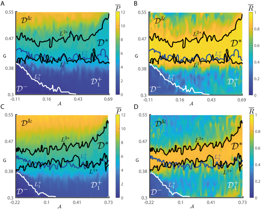
Finally, we considered weak coupling () for using realisations of the swapping algorithm. Figure S7 shows and when population 1 nodes account for (Fig. S7A,B) and (Fig. S7C,D) of the network. We found that non-monotonicity of the boundary to synchronised activity with respect to increasing was persistent for this weak coupling case. The upper boundary of the inter-population resonance regime (), given by the set , shows an increasing trend with respect to both when population 1 node comprise (Fig. S7B) and (Fig. S7D) of the network. Moreover, we again found that the activation threshold for population 1 nodes with respect to decreases as increases, which is captured by , where for . Interestingly, we found that the activation of population 2 nodes (reflected by ) with respect to shows a decreasing trend as increases, but only for very low values of . We conjecture that this relationship was not observed in Sec. III.1.3 because only positive values of (resulting from the forward algorithm) were considered there, whereas here we also include realisations of the backward algorithm (leading to negative values of being considered). Here, we found that the bounds of , those being and , needed to be modified depending on the proportion of population 1 nodes in the network. In particular, when only of the network nodes were from population 1, we defined the level set as in Sec. III.1.3 which subsequently led to the definition of two curves: the lower bound and the upper bound (Fig. S7B). However, when the proportion of population 1 nodes was increased to , we instead defined (Fig. S7D). The thresholds we chose were dependent on the number of population 2 nodes. This is because we sought to define level sets that bounded the 2:1 resonance region. In that region, nodes are synchronised within, but not between, populations. Therefore, is approximately equal to the fraction of nodes in the larger population (i.e., population 2).
S1.7 Additional figures referenced in the manuscript


