Generalized sparse Bayesian learning and application to image reconstruction Thanks: \monthyeardateAugust 11, 2026\correspondingJan Glaubitz

To address these issues, we present a generalized approach to SBL for “almost” general forward and regularization operators, $F$ and $R$. By “almost” general, we mean that the only restriction on $F$ and $R$ is that their common kernel should be trivial, $\kernel(F)\cap\kernel(R)=\{\mathbf{0}\}$, a standard assumption in regularized inverse problems [41]. We propose an efficient numerical method for Bayesian inference that yields a full conditional posterior density $p(\mathbf{x}|\mathbf{y})$, rather than a simple point estimate, which allows for uncertainty quantification in the solution $\mathbf{x}$. The present work implies that SBL can be applied to a broader class of problems than currently known. In particular, some preliminary results on signal and image reconstruction indicate its potential use for denoising, deblurring, and magnetic resonance imaging.

The rest of this paper is organized as follows. Section 2 provides some details on the sparsity promoting hierarchical Bayesian model under consideration. In section 3, we propose an efficient numerical method for Bayesian inference. A series of numerical examples is presented in section 4 to illustrate the descriptive span of the hierarchical Bayesian model. Finally, in section 5, we provide some concluding thoughts.

The likelihood function $p(\mathbf{y}|\mathbf{x},\bm{\alpha})$ models the connection between the solution $\mathbf{x}$, the noise parameters $\bm{\alpha}$, and the indirect measurements $\mathbf{y}$. It is often assumed that $\bm{\nu}\in\mathbb{R}^{m}$ in eq. 1 is zero-mean i. i. d. normal noise with inverse variance $\alpha>0$, that is, $\bm{\nu}\sim\mathcal{N}(\mathbf{0},\alpha^{-1}I)$. This assumption yields the conditionally Gaussian likelihood function

The likelihood function given by eq. 5 was considered, for instance, in [54, 19, 5, 6, 23]. By contrast, we restrict $\bm{\nu}$ to be independent but not necessarily identically distributed. This translates into ${\bm{\nu}\sim\mathcal{N}(\mathbf{0},A^{-1})}$ with diagonal positive definite inverse noise covariance matrix

The linear data model eq. 1 then yields the generalized likelihood function

which reduces to eq. 5 if the inverse variances $\alpha_{1},\dots,\alpha_{m}$ are all equal to $\alpha$. We note that conditionally Gaussian likelihoods of the form eq. 7 were considered in [15, Example 3.4] in combination with smoothness promoting priors to address data outliers. example 1 below motivates the weaker assumption ${\bm{\nu}\sim\mathcal{N}(\mathbf{0},A^{-1})}$ for sparsity promoting priors in the context of data fusion [37] and multi-sensor acquisition systems [36, 21].

The prior function $p(\mathbf{x}|\bm{\beta})$ models our prior belief about the unknown solution $\mathbf{x}$. Assume that some linear transformation of $\mathbf{x}$, say $R\mathbf{x}$, is sparse. The SBL approach promotes this assumed sparsity by using a conditionally Gaussian prior function,

where $B=\diag(\beta_{1},\dots,\beta_{k})$ is referred to as the inverse prior convariance matrix. See [54, 57, 19, 12, 18, 7, 5, 16, 22, 23] and references therein. The conditionally Gaussian prior eq. 11 can be justified by its asymptotic behavior [12]. If we assume that the inverse variances $\beta_{1},\dots,\beta_{k}$ are all equal, then eq. 11 favors solutions $\mathbf{x}$ for which $R\mathbf{x}$ is equal or close to zero,²² 2 For this prior, $R\mathbf{x}$ being close to zero means that $R\mathbf{x}$ has a small (unweighted) $\ell^{2}$-norm, $\|R\mathbf{x}\|_{2}$. since these solutions have a higher probability. For instance, when $R\mathbf{x}$ corresponds to the total variation of $\mathbf{x}$, $[R\mathbf{x}]_{j}=x_{j+1}-x_{j}$, then eq. 11 promotes solutions $\mathbf{x}$ that have no or little variation. However, if one of the inverse variances, say $\beta_{j}$, is significantly smaller than the remaining ones, a jump between $x_{j}$ and $x_{j+1}$ becomes more likely. In this way, eq. 11 promotes sparsity of $R\mathbf{x}$.

From the discussion above it is evident that the inverse variances $\beta_{1},\dots,\beta_{k}$ must be allowed to have distinctly different values for the conditionally Gaussian prior eq. 11 to promote sparsity of $R\mathbf{x}$. This can be achieved by treating $\beta_{1},\dots,\beta_{k}$ as random variables with uninformative density functions. A common choice is the gamma distribution with probability density function

where $c$ and $d$ are positive shape and rate parameters. Furthermore, $\Gamma(\cdot)$ on the right-hand side of eq. 12 denotes the usual gamma function [3]. Note that a gamma-distributed random variable, $X\sim\Gamma(c,d)$, respectively has mean $E[X]=c/d$ and variance $V[X]=c/d^{2}$. In particular, $c\to 1$ and $d\to 0$ implies $E[X],V[X]\to\infty$, making eq. 12 an uninformative prior. We therefore choose the inverse noise and prior variances, $\bm{\alpha}$ and $\bm{\beta}$, to be gamma-distributed:

By setting $c=1$ and $d\approx 0$, $\bm{\alpha}$ and $\bm{\beta}$ are free from the moderating influence of the hyper-prior and allowed to “vary wildly” following the data. In our numerical tests we used $d=10^{-4}$ for all one-dimensional problems (signals) and $d=10^{-2}$ for all two-dimensional problems (images), which is similar to the choices in [54, 5, 6]. Future investigations will elaborate on the influence of these parameters. A few remarks are in order.

The conditionally Gaussian prior eq. 11 and the gamma hyper-prior eq. 12 were intentionally chosen because of their conditional conjugacy relationship. Some especially important implications include the following (see [33]):

Here the covariance matrix $C$ and the mean $\bm{\mu}$ in eq. 14 are respectively given by

$[F\mathbf{x}-\mathbf{y}]_{i}$ denotes the $i$th entry of the vector $F\mathbf{x}-\mathbf{y}\in\mathbb{R}^{m}$, and $[R\mathbf{x}]_{j}$ denotes the $j$th entry of the vector $R\mathbf{x}\in\mathbb{R}^{k}$. Note that the two sides of eq. 14, eq. 15, and eq. 16 are equal up to a multiplicative constant that does not depend on $\mathbf{x}$, $\bm{\alpha}$, and $\bm{\beta}$, respectively. Finally, we stress that eq. 14 only holds if the forward operator $F\in\mathbb{R}^{m\times n}$ and the regularization operator $R\in\mathbb{R}^{k\times n}$ satisfy the common kernel condition:

which is a standard assumption in regularized inverse problems [41, 53]. Indeed, eq. 18 can be interpreted as the prior (regularization) introducing a sufficient amount of complementary information to the likelihood (the given measurements) to make the problem well-posed. This indicates that the hierarchical Bayesian model proposed in section 2 does not require $R$ to be invertible as long as eq. 18 is satisfied.

We are now in a position to formulate a Bayesian inference method for the generalized hierarchical Bayesian model from section 2. This method is motivated by the coordinate descent approaches [32, 58] and solves for a descriptive quantity (mode, mean, variance, etc.) of the posterior density function $p(\mathbf{x},\bm{\alpha},\bm{\beta}|\mathbf{y})$ by alternatingly updating this quantity for $\mathbf{x}$, $\bm{\alpha}$, and $\bm{\beta}$. Henceforth we refer to this method as the Bayesian coordinate descent (BCD) algorithm .

Assume that we are interested in the expected value (mean) of the posterior, $E[\mathbf{x},\bm{\alpha},\bm{\beta}|\mathbf{y}]$. The BCD algorithm for this case is described in algorithm 1.

In algorithm 1 and henceforth, all variables with superscripts are treated as fixed parameters. That is, the expected values in algorithm 1 are respectively computed w. r. t. $\mathbf{x}$, $\bm{\alpha}$, and $\bm{\beta}$. algorithm 1 is simple to implement because of the particular decomposition of the posterior density function $p(\mathbf{x},\bm{\alpha},\bm{\beta}|\mathbf{y})$ provided by Bayes’ theorem (see eq. 3):

By eqs. 14, 15, and 16, we therefore have

where the covariance matrix $C$ and the mean $\bm{\mu}$ in eq. 20 are given as in eq. 17 with $A=\diag(\bm{\alpha}^{l})$ and $B=\diag(\bm{\beta}^{l})$. Thus, the update step for $\mathbf{x}$ in algorithm 1 reduces to solving the linear system

for the mean $\mathbf{x}^{l+1}$, and the subsequent update steps for $\bm{\alpha}$ and $\bm{\beta}$ yield

respectively. Hence, algorithm 1 consists of alternating between eqs. 23, 24, and 25.

If the common kernel condition eq. 18 is satisfied, then the coefficient matrix on the left-hand side of eq. 23 is symmetric and positive definite (SPD). For sufficiently small problems, eq. 23 can therefore be solved efficiently using a preconditioned conjugate gradient (PCG) method [49]. However, the coefficient matrix may become prohibitively large in some cases. To avoid any potential storage and computational issues, we implemented our method using gradient descent for the imaging problems described in section 4.

Let $G=F^{T}AF+R^{T}BR$ and $\mathbf{b}=F^{T}A\mathbf{y}$ be the SPD coefficient matrix and the right-hand side of the linear system eq. 23, respectively. The solution of eq. 23 then corresponds to the unique minimizer of the quadratic functional

For this functional, line search minimization can be performed analytically to find the locally optimal step size $\gamma$ in every iteration. This allows us to use the classical gradient descent method described in algorithm 2 to approximate the solution $\mathbf{x}^{l+1}$ of eq. 23.

It is important to note that the gradient in eq. 28 can be computed efficiently and without having to store the whole coefficient matrix $G$, which might be prohibitively large. To show this, assume that the unknown solution $\mathbf{x}\in\mathbb{R}^{n^{2}}$ corresponds to a vectorized matrix $X\in\mathbb{R}^{n\times n}$ and that the forward operator $F$ corresponds to applying the same one-dimensional forward operator $F_{1}$ to the matrix $X$ in $x$- and $y$-direction:

where $F=F_{1}\otimes F_{1}$, $\mathbf{x}=\,\mathrm{vec}(X)$, and $\mathbf{y}=\,\mathrm{vec}(Y)$. We furthermore assume that the regularization operator $R$ is defined by

which corresponds to anisotropic regularization. Using some basic properties of the Kronecker product and the element-wise Hadamard product $\odot$, it can be shown that

where $\tilde{A}$, $\tilde{B}_{1}$, and $\tilde{B}_{2}$ are such that $\,\mathrm{vec}(\tilde{A})=\bm{\alpha}$, $\,\mathrm{vec}(\tilde{B}_{1})=\bm{\beta}^{1}$, and $\,\mathrm{vec}(\tilde{B}_{2})=\bm{\beta}^{2}$, with $\bm{\beta}=[\bm{\beta}^{1},\bm{\beta}^{2}]$. Combining eqs. 31, 32, and 33 yields

and therefore

Observe that all of the matrices in eqs. 34 and 35 are significantly smaller than $F$ and $R$.

The proposed BCD algorithm has the advantage of allowing for uncertainty quantification in the reconstructed solution $\mathbf{x}$. For fixed $\bm{\alpha}$ and $\bm{\beta}$, Bayes’ theorem and the conjugacy relationship eq. 14 yield

where the mean $\bm{\mu}$ and the covariance matrix $C$ are again given by eq. 17. We can then sample from the normal distribution $\mathcal{N}(\bm{\mu},C)$ to obtain, for instance, credible intervals for every component of the solution $\mathbf{x}$. At the same time, we stress that this only allows for uncertainty quantification in $\mathbf{x}$ for given hyper-parameters $\bm{\alpha}$ and $\bm{\beta}$. The above approach does not include uncertainty in $\bm{\alpha}$ and $\bm{\beta}$ when these are treated as random variables themselves. This might be achieved by employing a computational more expensive sampling approach [6], which we will investigate in future work.

We now address the connection between the proposed BCD algorithm and some existing methods.

We start with addressing the computational complexity of the proposed BCD algorithm (algorithm 1) for Bayesian inference. Assume that algorithm 1 stops after $L$ iterations, either because the algorithm has converged or reached the maximum number of iterations. In every iteration, the algorithm performs the $\mathbf{x}$-update eq. 23, the $\mathbf{\alpha}$-update eq. 24, and the $\bm{\beta}$-update eq. 25. Denoting their computational complexity by $\mathcal{O}(h_{x})$, $\mathcal{O}(h_{\alpha})$, and $\mathcal{O}(h_{\beta})$, respectively, the total computational complexity of the BCD method is $\mathcal{O}(L(h_{x}+h_{\alpha}+h_{\beta}))$.

Consider the sparse nodal values $\mathbf{x}$ of a signal $x\mathrel{\mathop{\ordinarycolon}}[0,1]\to\mathbb{R}$ at $n=20$ equidistant points. All of the values in $\mathbf{x}$ are zero except at four randomly selected locations, where the values were set to $1$. We are given noisy observations $\mathbf{y}$ which result from adding i. i. d. zero-mean normal noise with variance $\sigma^{2}=5\cdot 10^{-2}$ to the exact values $\mathbf{x}$. The signal-to-noise ratio (SNR), defined as $E[\mathbf{x}^{2}]/\sigma^{2}$ with $E[\mathbf{x}^{2}]=(x_{1}^{2}+\dots+x_{n}^{2})/n$, is $4$.

fig. 2(a) illustrates the exact values of $x$ and the noisy observations $\mathbf{y}$. The corresponding data model and regularization operator are

This simple test case allows us to compare the proposed BCD algorithm with some existing methods, some of which assume $\mathbf{x}$ itself to be sparse ($R=I$). fig. 2(b) provides a comparison of the BCD algorithm with (1) SBL using the evidence approach [54], (2) the IAS method [13, 12] solving for the MAP estimate of the posterior, and (3) the alternating direction method of multipliers (ADMM) [8] solving the deterministic $\ell^{1}$-regularized problem eq. 2. The free parameters of the IAS algorithm were fine-tuned by hand and chosen as $\beta=1.55$ and $\theta_{j}^{*}=5\cdot 10^{-2}$ for $j=1,\dots,n$; see [16] for more details on these parameters. The regularization parameter $\lambda$ in eq. 2 was also fine-tuned by hand and set to $\lambda=2\sigma^{2}\|\mathbf{x}\|_{0}$. Finally, for the proposed BCD algorithm and the evidence approach, we assumed the noise variance $\sigma^{2}$ to be unknown, which therefore had to be estimated by the method as well. We can see in fig. 2(b) that for this example all of the SBL-based methods perform similarly. On the other hand, the ADMM yeilds a more regularized reconstruction, which might be explained by the uniform nature of the $\ell^{1}$-regularization term in eq. 2. This is in contrast to the hierarchical Bayesian model which allows for spatially varying regularization. In this regard we note that there are weighted $\ell_{1}$-regularization methods [17, 20, 1] that incorporate spatially varying regularization parameters. While such techniques can improve the resolution near the non-zero values in sparse signals, as well as near the internal edges in images, they are still point estimates and thus do not provide additional uncertainty information. Hence in the current investigation we simply employ the standard ADMM with a fine-tuned non-varying regularization parameter as a reasonable comparison.

We next consider deconvolution of the piecewise constant signal $x\mathrel{\mathop{\ordinarycolon}}[0,1]\to\mathbb{R}$ illustrated in fig. 3. The corresponding data model and regularization operator are respectively given by

where $\bm{\nu}\sim\mathcal{N}(\mathbf{0},\sigma^{2}I)$ with $\sigma^{2}=10^{-2}$ ($\mathrm{SNR}\approx 80$) and $F$ is obtained by applying the midpoint quadrature to the convolution equation

We assume a Gaussian convolution kernel of the form

with blurring parameter $\gamma=3\cdot 10^{-2}$. The forward operator thus is

where $h=1/n$ is the distance between consecutive grid points. Note that $F$ has full rank but quickly becomes ill-conditioned.

fig. 3(a) illustrates the true signal $x$ as well as the given noisy blurred data $\mathbf{y}$ at $n=40$ equidistant points. fig. 3(b) provides the reconstructions using the SBL-based BCD algorithm and the ADMM $\ell^{1}$-regularized inverse problem eq. 2. The regularization parameter $\lambda$ in eq. 2 was again fine-tuned by hand and chosen as $\lambda=2\sigma^{2}\|R\mathbf{x}\|_{0}$. We do not include any of the existing SBL algorithms considered before (the evidence approach and IAS algorithm) since they cannot be applied to the non-quadratic regularization operator $R$ in eq. 38 without modifying this operator first. fig. 3(c) illustrates the normalized prior covariance parameters $\beta^{-1}$ which are estimated as part of the BCD algorithm. Observe that the values are significantly larger at the locations of the jump discontinuities. This allows the reconstruction to “jump” and highlights the nonuniform character of regularization in the hierarchical Bayesian model suggested in section 2. Finally, fig. 3(d) demonstrates the possibility to quantify uncertainty when using the BCD algorithm by providing the $99.9\%$ credible intervals of the solution posterior $p(\mathbf{x}|\mathbf{y})$ for the final estimates of $\alpha$ and $\bm{\beta}$. Note that these credible intervals, especially their width, indicate the amount of uncertainty in the reconstruction.

The results displayed in fig. 4 are for the same model with the noise variance increased by $500\%$, to $\sigma^{2}=5\cdot 10^{-2}$ ($\mathrm{SNR}\approx 16$). The BCD algorithm now yields a less accurate reconstruction, especially between $t=0.15$ and $t=0.25$. This is also reflected in the corresponding normalized prior covariance parameters $\beta^{-1}$, which can be found fig. 4(c). Observe that the second peak around $t=0.25$ is underestimated and therefore causes the block associated with the region $[0.15,0.25]$ to be drawn towards the subsequent block associated with the region $[0.25,0.5]$. The increased uncertainty of the reconstruction is indicated by the $99.9\%$ credible intervals in fig. 4(d). In particular, we note the increased width of the credible interval in the region $[0.15,0.25]$.

We next demonstrate that generalized SBL allows us to consider combinations of different regularization operators. Consider the signal $x\mathrel{\mathop{\ordinarycolon}}[0,1]\to\mathbb{R}$ illustrated in fig. 5(a), which is piecewise constant on $[0,0.5]$ and piecewise linear on $[0.5,1]$. The corresponding data model is the same as before with convolution parameter $\gamma=10^{-2}$ and i. i. d. zero-mean normal noise with variance $\sigma^{2}=10^{-2}$ ($\mathrm{SNR}\approx 40$). fig. 5(b) illustrates the reconstructions obtained by the BCD algorithm using a first- and second-order TV-regualrization operator,

which promote piecewise constant and piecewise linear solutions, respectively. Observe that neither $R_{1}$ nor $R_{2}$ is even square, meaning that both would have to be modified by introducing additional rows to apply a standard SBL approach, which can become increasingly complicated for higher orders and multiple dimensions.

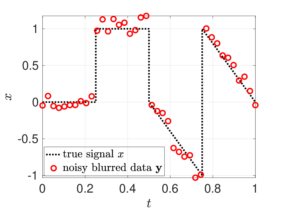
It is evident from fig. 5(b) that using first-order TV-regularization yields a less accurate reconstruction in $[0.5,1]$, where the signal is piecewise linear,⁷⁷ 7 This well-known artifact of first-order TV-regularization is often called the “staircasing” effect and motivates using higher order TV-regularization, [2, 52]. while using second-order TV-regularization yields a less accurate reconstruction in $[0,0.5]$, where the signal is piecewise constant. However, generalized SBL and the proposed BCD algorithm allows us to consider the combined regularization operator

Assuming $n=2q$, the first $k-1$ rows correspond to first-order TV-regularization while the last $k-2$ rows correspond to second-order TV-regularization. The advantage of using this nonstandard regularization operator in the BCD algorithm is demonstrated by the red stars in fig. 5(b).

We next consider the reference image $X$ in fig. 6(a) and its noisy blurred version $Y$ in fig. 6(b). $Y$ results from $X$ by applying the discrete one-dimensional convolution operator eq. 41 in the two canonical coordinate directions and then adding i. i. d. zero-mean normal noise. The corresponding forward model is $Y=FXF^{T}+N$ or, equivalently,

after vectorization. Here, $\mathbf{z}=\vec{(}Z)$ denotes the $mn\times 1$ column vectors obtained by stacking the columns of the $m\times n$ matrix $Z$ on top of one another, and $G=F\otimes F$. Further, the blurring parameter and noise variance were chosen as $\gamma=1.5\cdot 10^{-2}$ and $\sigma^{2}=10^{-5}$ ($\mathrm{SNR}\approx 4\cdot 10^{3}$) to make the test case comparable to the one in [6, Section 4.2].

figs. 6(c) and 6(d) show the reconstructions obtained by the ADMM applied to eq. 2 and the SBL-based BCD algorithm with an anisotropic second-order TV operator

The regularization parameter $\lambda$ in eq. 2 was again fine-tuned by hand and set to $\lambda=10^{-5}$. The BCD algorithm provides a sharper reconstruction (see fig. 6) than the ADMM applied to the $\ell^{1}$-regularized inverse problem eq. 2. Further parameter tuning might increase the accuracy of the reconstruction by the ADMM. By contrast, it is important to stress that the BCD algorithm requires no such exhaustive parameter tuning.

We next address the reconstruction of images based on noisy and incomplete Fourier data, which is common in applications such as magnetic resonance imaging (MRI) and synthetic aperture radar (SAR). The popular prototype Shepp–Logan phantom test image is displayed in fig. 7(a).

The indirect data $\mathbf{y}=\vec{(}Y)$ is given by applying the two-dimensional discrete Fourier transform to the reference image $X$, removing certain frequencies, and adding noise. Since in this investigation we are assuming $\mathbf{x}\in\mathbb{R}^{n}$, we consider the data model

with $\mathrm{Re}(\mathbf{y})$ and $\mathrm{Im}(\mathbf{y})$ respectively denoting the real and imaginary part of $\mathbf{y}\in\mathbb{C}^{m}$.⁸⁸ 8 Our technique is not limited to real-valued solutions, and we will consider complex-valued solutions, such as those occurring in SAR, in future work. Further, $\bm{\nu}\in\mathbb{R}^{2m}$ corresponds to i. i. d. zero-mean normal noise with variance $\sigma^{2}=10^{-3}$ ($\mathrm{SNR}\approx 60$) and $G=F\otimes F$, where $F$ denotes the one-dimensional discrete Fourier transform with missing frequencies, which we impose to mimic the situation where the system is under-determined and some data must for some reason be discarded. The removed frequencies were determined by sampling $100$ logarithmically spaced integers between $10$ and $200$. Finally, because the image is piecewise constant, we used first-order TV-regularization.

fig. 7(b) shows the maximum likelihood (ML) estimate of the image, which is obtained by maximizing the likelihood function $p(\mathbf{x}|\mathbf{y})$. In this case, the ML estimate is the same as the least squares (LS) solution of the linear system eq. 46. figs. 7(c) and 7(d) illustrate the reconstructions obtained by applying ADMM to the $\ell^{1}$-regularized inverse problem eq. 2 and the SBL-based BCD algorithm. The regularization parameter in eq. 2 was again fine-tuned by hand and chosen as $\lambda=4\sigma^{2}$. While the reconstructions in figs. 7(c) and 7(d) are comparable, it is important to point out that we did not use any prior knowledge about the noise variance or perform any parameter tuning for the BCD algorithm.

As a final example we consider a data fusion problem to demonstrate the possible advantage of using the generalized noise model discussed in section 2.1. Recall the piecewise constant signal discussed in section 4.3, and assume we want to reconstruct the values of this signal at $n=40$ equidistant grid points, denoted by $\mathbf{x}$. We are given two sets of data: $\mathbf{y}^{(1)}$ corresponds to direct observations taken at $36$ randomly selected locations with added i. i. d. zero-mean normal noise $\bm{\nu}^{(1)}$ with variance $\sigma_{1}^{2}=5\cdot 10^{-1}$, and $\mathbf{y}^{(2)}$ corresponds to blurred observations at $24$ randomly selected locations with added i. i. d. zero-mean normal noise $\bm{\nu}^{(2)}$ with variance $\sigma_{2}^{2}=10^{-2}$. The blurring is again modeled using eq. 41 with a Gaussian convolution kernel and convolution parameter $\gamma=3\cdot 10^{-2}$. Further, a first-order TV-regularization operator is employed to promote a piecewise constant reconstruction.

The separate reconstructions by the SBL-based BCD algorithm can be found in figs. 8(a) and 8(b). Both reconstructions are of poor quality, which is due to the high noise variance in the case of $\mathbf{y}^{(1)}$ and to the missing information in the case of $\mathbf{y}^{(2)}$. In fact, the reconstruction illustrated in fig. 8(b) is of reasonable quality except for the region around $t=0.2$, where a void of observations causes the reconstruction to miss the jumps at $t=0.15$ and $t=0.25$.

Following example 1, we now fuse the two data sets by considering the joint data model

References

- [1] B. Adcock, A. Gelb, G. Song, and Y. Sui, Joint sparse recovery based on variances, SIAM Journal on Scientific Computing, 41 (2019), pp. A246–A268.
- [2] R. Archibald, A. Gelb, and R. B. Platte, Image reconstruction from undersampled Fourier data using the polynomial annihilation transform, Journal of Scientific Computing, 67 (2016), pp. 432–452.
- [3] E. Artin, The Gamma Function, Courier Dover Publications, 2015.
- [4] S. D. Babacan, R. Molina, and A. K. Katsaggelos, Parameter estimation in TV image restoration using variational distribution approximation, IEEE Transactions on Image Processing, 17 (2008), pp. 326–339.
- [5] S. D. Babacan, R. Molina, and A. K. Katsaggelos, Sparse Bayesian image restoration, in 2010 IEEE International Conference on Image Processing, IEEE, 2010, pp. 3577–3580.
- [6] J. M. Bardsley, MCMC-based image reconstruction with uncertainty quantification, SIAM Journal on Scientific Computing, 34 (2012), pp. A1316–A1332.
- [7] J. M. Bardsley, D. Calvetti, and E. Somersalo, Hierarchical regularization for edge-preserving reconstruction of PET images, Inverse Problems, 26 (2010), p. 035010.
- [8] S. Boyd, N. Parikh, and E. Chu, Distributed optimization and statistical learning via the alternating direction method of multipliers, Now Publishers Inc, 2011.
- [9] D. Calvetti, A. Pascarella, F. Pitolli, E. Somersalo, and B. Vantaggi, A hierarchical Krylov–Bayes iterative inverse solver for MEG with physiological preconditioning, Inverse Problems, 31 (2015), p. 125005.
- [10] D. Calvetti, M. Pragliola, and E. Somersalo, Sparsity promoting hybrid solvers for hierarchical Bayesian inverse problems, SIAM Journal on Scientific Computing, 42 (2020), pp. A3761–A3784.
- [11] D. Calvetti, M. Pragliola, E. Somersalo, and A. Strang, Sparse reconstructions from few noisy data: analysis of hierarchical Bayesian models with generalized gamma hyperpriors, Inverse Problems, 36 (2020), p. 025010.
- [12] D. Calvetti and E. Somersalo, A Gaussian hypermodel to recover blocky objects, Inverse Problems, 23 (2007), p. 733.
- [13] D. Calvetti and E. Somersalo, An Introduction to Bayesian Scientific Computing: Ten Lectures on Subjective Computing, vol. 2, Springer Science & Business Media, 2007.
- [14] D. Calvetti and E. Somersalo, Hypermodels in the Bayesian imaging framework, Inverse Problems, 24 (2008), p. 034013.
- [15] D. Calvetti and E. Somersalo, Subjective knowledge or objective belief? an oblique look to Bayesian methods, Large-Scale Inverse Problems and Quantification of Uncertainty, (2010), pp. 33–70.
- [16] D. Calvetti, E. Somersalo, and A. Strang, Hierachical Bayesian models and sparsity: -magic, Inverse Problems, 35 (2019), p. 035003.
- [17] E. J. Candès, M. B. Wakin, and S. P. Boyd, Enhancing sparsity by reweighted minimization, Journal of Fourier Analysis and Applications, 14 (2008), pp. 877–905.
- [18] G. Chantas, N. Galatsanos, A. Likas, and M. Saunders, Variational Bayesian image restoration based on a product of -distributions image prior, IEEE Transactions on Image Processing, 17 (2008), pp. 1795–1805.
- [19] G. K. Chantas, N. P. Galatsanos, and A. C. Likas, Bayesian restoration using a new nonstationary edge-preserving image prior, IEEE Transactions on Image Processing, 15 (2006), pp. 2987–2997.
- [20] R. Chartrand and W. Yin, Iteratively reweighted algorithms for compressive sensing, in IEEE International Conference on Acoustics, Speech and Signal Processing, 2008, pp. 3869–3872.
- [21] I. Y. Chun and B. Adcock, Compressed sensing and parallel acquisition, IEEE Transactions on Information Theory, 63 (2017), pp. 4860–4882.
- [22] V. Churchill and A. Gelb, Detecting edges from non-uniform Fourier data via sparse Bayesian learning, Journal of Scientific Computing, 80 (2019), pp. 762–783.
- [23] V. Churchill and A. Gelb, Estimation and uncertainty quantification for piecewise smooth signal recovery, Journal of Computational Mathematics, 41 (2022).
- [24] D. Colton, M. Piana, and R. Potthast, A simple method using Morozov’s discrepancy principle for solving inverse scattering problems, Inverse Problems, 13 (1997), p. 1477.
- [25] I. Daubechies, R. DeVore, M. Fornasier, and C. S. Güntürk, Iteratively reweighted least squares minimization for sparse recovery, Communications on Pure and Applied Mathematics: A Journal Issued by the Courant Institute of Mathematical Sciences, 63 (2010), pp. 1–38.
- [26] D. L. Donoho, Compressed sensing, IEEE Transactions on Information Theory, 52 (2006), pp. 1289–1306.
- [27] Y. C. Eldar and G. Kutyniok, Compressed Sensing: Theory and Applications, Cambridge University Press, 2012.
- [28] R. Fergus, B. Singh, A. Hertzmann, S. T. Roweis, and W. T. Freeman, Removing camera shake from a single photograph, in ACM SIGGRAPH 2006 Papers, 2006, pp. 787–794.
- [29] M. A. Figueiredo, J. M. Bioucas-Dias, and R. D. Nowak, Majorization–minimization algorithms for wavelet-based image restoration, IEEE Transactions on Image Processing, 16 (2007), pp. 2980–2991.
- [30] D. Fink, A compendium of conjugate priors, 46 (1997), https://www.johndcook.com/CompendiumOfConjugatePriors.pdf.
- [31] S. Foucart and H. Rauhut, A mathematical introduction to compressive sensing, Bull. Am. Math, 54 (2017), pp. 151–165.
- [32] J. Friedman, T. Hastie, and R. Tibshirani, Regularization paths for generalized linear models via coordinate descent, Journal of Statistical Software, 33 (2010), p. 1.
- [33] A. Gelman, J. B. Carlin, H. S. Stern, and D. B. Rubin, Bayesian Data Analysis, Chapman and Hall/CRC, third ed., 2021, http://www.stat.columbia.edu/~gelman/book/.
- [34] G. H. Golub, M. Heath, and G. Wahba, Generalized cross-validation as a method for choosing a good ridge parameter, Technometrics, 21 (1979), pp. 215–223.
- [35] C. W. Groetsch and C. Groetsch, Inverse Problems in the Mathematical Sciences, vol. 52, Springer, 1993.
- [36] M. Guerquin-Kern, L. Lejeune, K. P. Pruessmann, and M. Unser, Realistic analytical phantoms for parallel magnetic resonance imaging, IEEE Transactions on Medical Imaging, 31 (2011), pp. 626–636.
- [37] F. Gustafsson, Statistical Sensor Fusion, Studentlitteratur, 2010.
- [38] P. C. Hansen, The L-curve and its use in the numerical treatment of inverse problems, (1999).
- [39] P. C. Hansen, Discrete Inverse Problems: Insight and Algorithms, SIAM, 2010.
- [40] P. C. Hansen, J. G. Nagy, and D. P. O’leary, Deblurring Images: Matrices, Spectra, and Filtering, SIAM, 2006.
- [41] J. Kaipio and E. Somersalo, Statistical and Computational Inverse Problems, vol. 160, Springer Science & Business Media, 2006.
- [42] J. P. Kaipio, V. Kolehmainen, E. Somersalo, and M. Vauhkonen, Statistical inversion and Monte Carlo sampling methods in electrical impedance tomography, Inverse Problems, 16 (2000), p. 1487.
- [43] D. Krishnan and R. Fergus, Fast image deconvolution using hyper-Laplacian priors, Advances in Neural Information Processing Systems, 22 (2009), pp. 1033–1041.
- [44] A. Lanza, M. Pragliola, and F. Sgallari, Residual whiteness principle for parameter-free image restoration, Electronic Transactions on Numerical Analysis, 53 (2020), pp. 329–351.
- [45] A. Levin, R. Fergus, F. Durand, and W. T. Freeman, Image and depth from a conventional camera with a coded aperture, ACM Transactions on Graphics (TOG), 26 (2007), pp. 70–es.
- [46] D. J. MacKay, Bayesian interpolation, Neural Computation, 4 (1992), pp. 415–447.
- [47] K. P. Murphy, Conjugate Bayesian analysis of the Gaussian distribution, (2007), https://www.cs.ubc.ca/~murphyk/Papers/bayesGauss.pdf.
- [48] F. Natterer and F. Wübbeling, Mathematical Methods in Image Reconstruction, SIAM, 2001.
- [49] Y. Saad, Iterative Methods for Sparse Linear Systems, SIAM, 2003.
- [50] T. Sanders, R. B. Platte, and R. D. Skeel, Effective new methods for automated parameter selection in regularized inverse problems, Applied Numerical Mathematics, 152 (2020), pp. 29–48.
- [51] H. Stark, Image Recovery: Theory and Application, Elsevier, 2013.
- [52] W. Stefan, R. A. Renaut, and A. Gelb, Improved total variation-type regularization using higher order edge detectors, SIAM Journal on Imaging Sciences, 3 (2010), pp. 232–251.
- [53] A. N. Tikhonov, A. Goncharsky, V. Stepanov, and A. G. Yagola, Numerical Methods for the Solution of Ill-Posed Problems, vol. 328 of Mathematics and Its Applications, Springer Science & Business Media, 2013.
- [54] M. E. Tipping, Sparse Bayesian learning and the relevance vector machine, Journal of Machine Learning Research, 1 (2001), pp. 211–244.
- [55] C. R. Vogel, Computational Methods for Inverse Problems, SIAM, 2002.
- [56] D. Wipf and S. Nagarajan, A new view of automatic relevance determination, Advances in Neural Information Processing Systems, 20 (2007).
- [57] D. P. Wipf and B. D. Rao, Sparse Bayesian learning for basis selection, IEEE Transactions on Signal processing, 52 (2004), pp. 2153–2164.
- [58] S. J. Wright, Coordinate descent algorithms, Mathematical Programming, 151 (2015), pp. 3–34.
- [59] Z. Zhang, T.-P. Jung, S. Makeig, Z. Pi, and B. D. Rao, Spatiotemporal sparse Bayesian learning with applications to compressed sensing of multichannel physiological signals, IEEE Transactions on Neural Systems and Rehabilitation Engineering, 22 (2014), pp. 1186–1197.
- [60] Z. Zhang and B. D. Rao, Clarify some issues on the sparse Bayesian learning for sparse signal recovery, University of California, San Diego, Tech. Rep, (2011).
- [61] Z. Zhang and B. D. Rao, Sparse signal recovery with temporally correlated source vectors using sparse Bayesian learning, IEEE Journal of Selected Topics in Signal Processing, 5 (2011), pp. 912–926.