Target-enclosing inversion using an interferometric objective functionVolume: 200

We set up the inverse problem in the constant density acoustic formulation for pressure $p$ and scaled particle displacement $\mathbf{u}=\rho\int_{t}\mathbf{v}$ in the time domain, so that $\mathbf{w}(\mathbf{x},\mathbf{x}_{s},t)=[p(\mathbf{x},\mathbf{x}_{s},t),\mathbf{u}(\mathbf{x},\mathbf{x}_{s},t)]$. Integral equations (1), (2) can be expressed as partial differential equations for pressure and scaled displacement using the forward and adjoint vector-acoustic differential operators (Zheglova & Malcolm 2020) and convolution and correlation areal sources along the boundary $\partial D$:

where:

$\mathbf{w}^{i}=[p^{i},\mathbf{u}^{i}]$, $i=\left\{conv,corr\right\}$ are the convolution and correlation pressure and particle displacement vector-acoustic wavefields;

$\mathbf{L}$ and $\mathbf{L}^{\dagger}$ are the vector-acoustic differential operator and its adjoint:

$\displaystyle\mathbf{L}(\mathbf{x},m)=\begin{pmatrix}m&\nabla^{T}\\ \nabla&\partial_{tt}\mathbf{I}\end{pmatrix},\;\;\;\mathbf{L}^{\dagger}(\mathbf{x},m)=\begin{pmatrix}m&-\nabla^{T}\\ -\nabla&\partial_{tt}\mathbf{I}\end{pmatrix};$

$m=1/c^{2}$ is the squared slowness;

$\mathbf{s}^{conv}$ and $\mathbf{s}^{corr}$ are the convolution and correlation sources given at each $\mathbf{x}_{r}\in\partial D$ as

	$\displaystyle\mathbf{s}^{conv}(\mathbf{x}_{r},t)$	$\displaystyle=$	$\displaystyle-\mathbf{N}_{r}(\mathbf{x}_{r})\mathbf{w}(\mathbf{x},\mathbf{x}_{s},t)=-\begin{pmatrix}\mathbf{n}(\mathbf{x}_{r})^{T}\mathbf{u}(\mathbf{x}_{r},\mathbf{x}_{s},t)\\ \mathbf{n}(\mathbf{x}_{r})\;p(\mathbf{x}_{r},\mathbf{x}_{s},t)\end{pmatrix}$
	$\displaystyle\mathbf{s}^{corr}(\mathbf{x}_{r},t)$	$\displaystyle=$	$\displaystyle-\mathbf{K}\mathbf{N}_{r}(\mathbf{x}_{r})\mathbf{w}(\mathbf{x},\mathbf{x}_{s},t)=\begin{pmatrix}-\mathbf{n}(\mathbf{x}_{r})^{T}\mathbf{u}(\mathbf{x}_{r},\mathbf{x}_{s},t)\\ \mathbf{n}(\mathbf{x}_{r})\;p(\mathbf{x}_{r},\mathbf{x}_{s},t)\end{pmatrix};$

$\delta_{\partial D}(\mathbf{x},\mathbf{x}_{r})$ denotes the areal source distributed along the boundary $\partial D$.

As per the time-domain adjoint-state approach, Equation (7) is solved forward in time, while equation (8) is solved backward in time.

Based on the reciprocity relations we discuss above, the objective function we use is

where $||\textbf{x}||_{2}^{2}=\sum_{i}x_{i}^{2}$ is the squared Euclidean $l_{2}$ norm and $\mitbf{\Lambda}$ is the data weighting operator. In this study we use

which samples only pressure. Note that here, unlike the representations in Eqs. 1 and 2, we use an explicit time-domain representation for the sake of consistency with our time-domain implementation of the adjoint-state vector-acoustic wave equations.

Equation (9) together with equations (7) and (8) constitute the PDE constrained optimization problem that we solve for the model parameter $m$.

We remark that the convolution and correlation differential equations (7) and (8) together constitute the forward problem that is exactly satisfied by the convolution and correlation fields. The (redatumed) data $\mathbf{w}(\mathbf{x}_{r},\mathbf{x}_{s},t)$ at the boundary $\partial D$ constitute the observed data. The convolution and correlation sources are fully determined by the redatumed data and the geometry of $\partial D$. Unlike in conventional surface FWI and local FWI, we do not directly compare the observed and modelled fields along a line of receivers. Rather, the modelled data are the pressures ${p^{corr}}=\mitbf{\Lambda}\mathbf{w}^{corr}$ and $p^{conv}=\mitbf{\Lambda}\mathbf{w}^{conv}$, whose difference must be zero everywhere in the local domain. This process can also be expressed as minimization of $\left\|\begin{pmatrix}\mitbf{\Lambda}&-\mitbf{\Lambda}\end{pmatrix}\begin{pmatrix}\mathbf{w}^{corr}&\mathbf{w}^{conv}\end{pmatrix}^{T}\right\|^{2}_{2}$. The implications of such an objective function are far wider than it may initially sound: by imposing equivalence between two wavefields, neither of them must be known directly at the location where the objective function in evaluated, allowing us to consider a grid within the entire domain of interest. When only one representation theorem is used (Cui et al. 2020, e.g.) the objective function can also be theoretically evaluated at any point in the grid; however, in practical application this would require being able to access the wavefield at such location by means of e.g., Marchenko redatuming, leading to a radical increase in the computational cost associated with the data preparation prior to inversion.

The gradient of the interferometric objective function with respect to the model parameter $m$ is derived by the adjoint state method (Plessix 2006; Fichtner 2011). We derive it in Appendix A, and show here only the result. In the general form, the gradient of the interferometric objective function with respect to the squared slowness $m$ is given by

where $\mathbf{w}^{conv\dagger}=\begin{pmatrix}p^{conv\dagger}\\ \mathbf{u}^{conv\dagger}\end{pmatrix}$ and $\mathbf{w}^{corr\dagger}=\begin{pmatrix}p^{corr\dagger}\\ \mathbf{u}^{corr\dagger}\end{pmatrix}$ are the adjoint convolution and correlations wavefields that satisfy the adjoint convolution and correlation equations:

Equations (11) and (12) are solved respectively backward and forward in time.

With the choice of $\mitbf{\Lambda}$ as in (10), the gradient becomes

Since the residual $\mathbf{w}^{corr}-\mathbf{w}^{conv}$ is calculated over the whole $D$, the convolution and correlation adjoint sources, i.e. right-hand sides of equations (11) and (12) are volume sources injected everywhere in the local domain. This is different from conventional FWI, where the adjoint sources are usually injected at the receiver locations. Similar to conventional FWI, the adjoint fields are computed in the opposite time direction to the forward problem, and zero-lag cross-correlations of the forward and adjoint fields are computed to obtain the gradient.

We implement the iterative inversion by combining the IFWI objective and gradient with the L-BFGS optimization method.

In this section, we investigate the convexity of the interferometric objective function in the target domain using exact data, and compare it to the surface FWI objective function. We consider an example, where we obtain the true model, shown in Figure 2, by applying a mask to a modified Marmousi model. We place six sources between 1 and 3 km in the horizontal direction at a depth of 0.1 km and use a Ricker wavelet with a peak frequency of 15 Hz as the source signature.

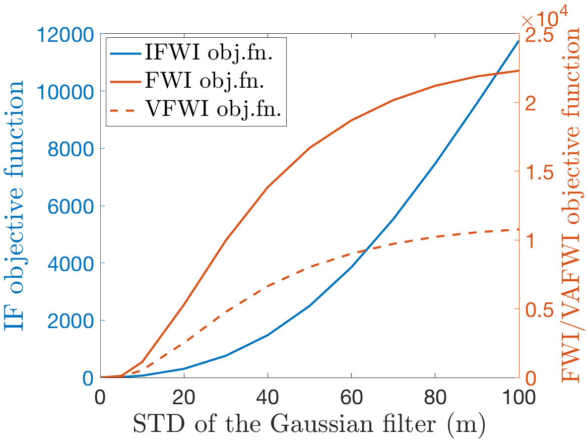
Because a kinematically accurate macro velocity model is usually needed for both full waveform inversion and redatuming, we are primarily interested in the response of the objective function to the lack of high wavenumber components in the model. Therefore, we apply 2D Gaussian smoothing to the target area, where we vary the standard deviation of the Gaussian filter from 5 to 100 m to obtain progressively smoother models of the target, and compute the objective function value for each of the smoothed models. Examples of such smoothed local models are shown in Figure 2 (b), (c). Figure 3 shows the interferometric objective function variation with the STD of the Gausian filter. For comparison, we show the surface FWI objective and vector-acoustic FWI (VAFWI) objective function (Zheglova & Malcolm 2020) for the same smoothed models. To compute the FWI and VAFWI objective, receivers are placed every 10 m between 0.2 and 3.8 km at depth 0.1 km. For the calculation of FWI and VAFWI objective function, we apply no smoothing to the overburden layer. Note that, apart from the difference in absolute values, the interferometric objective function is more convex than both the FWI and VAFWI objective functions, in addition, it has a wider basin of attraction near the global minimum. Based on this experiment, we can expect the IFWI to exhibit fast initial convergence with a subsequent slow-down near the minimum. We can also expect the IFWI to be more resistant to errors in the initial model, which we show to be case with exact data.

In this section, we take a closer look at the gradient of the interferometric objective function.

First, we observe that each of the two terms in the gradient (equation 13) is a zero-lag correlation of the forward field with the corresponding adjoint field. Each of the adjoint fields in turn consists of two parts: a part due to the convolution forward field, and a part due to the correlation forward field, as follows from the adjoint equations (11) and (12). We denote these adjoint field components as follows:

1. 1.

   $\mathbf{w}^{conv\dagger}_{conv}=\Gamma^{\dagger}\mitbf{\Lambda}^{\dagger}\mitbf{\Lambda}\Gamma w^{conv}$ is the part of the convolution adjoint field $\mathbf{w}^{conv\dagger}$ due to the convolution part of the adjoint source ${\mitbf{\Lambda}}^{\dagger}\mitbf{\Lambda}\mathbf{w}^{conv}$

2. 2.

   $\mathbf{w}^{conv\dagger}_{corr}=-\Gamma^{\dagger}\mitbf{\Lambda}^{\dagger}\mitbf{\Lambda}\Gamma^{\dagger}w^{corr}$ is the part of the convolution adjoint field $\mathbf{w}^{conv\dagger}$ due to the correlation part of the adjoint source $-{\mitbf{\Lambda}}^{\dagger}\mitbf{\Lambda}\mathbf{w}^{corr}$

3. 3.

   $\mathbf{w}^{corr\dagger}_{corr}=\Gamma\mitbf{\Lambda}^{\dagger}\mitbf{\Lambda}\Gamma^{\dagger}w^{corr}$ is the part of the correlation adjoint field $\mathbf{w}^{corr\dagger}$ due to the correlation part of the adjoint source ${\mitbf{\Lambda}}^{\dagger}\mitbf{\Lambda}\mathbf{w}^{corr}$, and

4. 4.

   $\mathbf{w}^{corr\dagger}_{conv}=\Gamma\mitbf{\Lambda}^{\dagger}\mitbf{\Lambda}\Gamma w^{corr}$ is the part of the correlation adjoint field $\mathbf{w}^{corr\dagger}$ due to the convolution part of the adjoint source $-{\mitbf{\Lambda}}^{\dagger}\mitbf{\Lambda}\mathbf{w}^{conv}$,

where $\Gamma$ and $\Gamma^{\dagger}$ are Green’s functions for operators $\mathbf{L}$ and $\mathbf{L}^{\dagger}$. Correspondingly, the four terms in the gradient are:

We use two starting models to analyze the behaviour of the IFWI gradient, shown in Figure 2 (b) and (c). The model in Figure 2 (b) represents late inversion stages, while the model in Figure 2 (c) represents early inversion stages. The original field is generated by a Ricker wavelet source with a peak frequency of 15 Hz located at the middle top of the model (Figure 2) at $z=0.1$ km, $x=2$ km.

First, we look at the gradient obtained in the starting model in Figure 2 (b). This model is very close to the true model and contains almost all of the high wavenumber details in the local subdomain.

Figures 4 (a) and (c) show the individual cross-correlation terms $\frac{\partial I}{\partial m}^{(i)}$ and $\frac{\partial I}{\partial m}^{(ii)}$ of the gradient, and Figure 4 (e) shows their sum. The two terms $\frac{\partial I}{\partial m}^{(i)}$ and $\frac{\partial I}{\partial m}^{(ii)}$ in Figure 4 (a) and (c) have reversed polarity in both low and high wavenumber components, which happens because the convolution and correlation forward fields in the adjoint sources have opposite signs. Due to the mismatch in the convolution and the correlation forward fields, these cross-correlation terms with opposite polarity are not exactly aligned and do not sum to zero, producing a pattern in the gradient that closely follows the features in the model perturbation. The same can be observed to a certain degree for the individual cross-correlation terms $\frac{\partial I}{\partial m}^{(iii)}$ and $\frac{\partial I}{\partial m}^{(iv)}$ shown in Figure 4 (b) and (d) and their sum shown in Figure 4 (f), although it is apparent that other mechanisms are also present in the correlation update. Thus, Figure 4 visually demonstrates that when the initial model is close to the starting model, the gradient update is driven by the mismatch in the convolution and correlation forward wavefields at the later stages of the inversion.

The situation is somewhat different for the starting model shown in Figure 2 (c). The individual cross-correlation terms and their sums for this model are shown in Figure 5. This model is very smooth and lacks any high-wavenumber details, so the convolution forward field does not undergo any scattering inside the local domain and is purely down-going: $p^{conv}\downarrow$. It also generates a purely down-going adjoint field $p^{conv\dagger}_{conv}\downarrow$ and a purely up-going field $p^{corr\dagger}_{conv}\uparrow$. Zero-lag correlation of the fields traveling in the same direction generates low-wavenumber updates, whereas zero-lag correlation of the fields travelling in opposite directions generates low-wavenumber updates. The term $\frac{\partial I}{\partial m}^{(i)}$ is a cross-correlation of two down going waves, and therefore updates only low wavenumbers, Figure 5 (a). The correlation field $p^{corr}$ has both transmitted and reflected waves from the true model that are respectively down- and up-going: $p^{corr}\downarrow+\uparrow$, and generates up- and down-going waves in the adjoint field components $p^{conv\dagger}_{corr}:\uparrow+\downarrow$ and $p^{corr\dagger}_{corr}:\uparrow+\downarrow$. Consequently, $\frac{\partial I}{\partial m}^{(ii)}$ contains zero-lag correlations of up- and down-going waves as well as down- and down-going waves: $\uparrow\downarrow+\downarrow\downarrow$ and therefore updates both low and high wavenumbers, Figure 5 (c). Likewise, the term $\frac{\partial I}{\partial m}^{(iv)}$ contains cross-correlations of the up- and up-going waves as well as up- and down-going waves $\uparrow\uparrow+\uparrow\downarrow$, Figure 5 (d). Finally $\frac{\partial I}{\partial m}^{(iii)}$ contains all possible cross-correlations: $\uparrow\uparrow+\uparrow\downarrow+\downarrow\uparrow+\downarrow\downarrow$ and updates all wavenumbers to some degree, Figure 5 (b).

The second observation we make from Figures 4 (e), (f) and 5 (e), (f) is that the convolution and correlation components in the gradient contribute to different parts of the model update. The convolution term $\int_{0}^{T}p^{conv}p^{conv\dagger}dt$, Figure 4 and 5 (c), updates the target area mostly above the bottom reflector of the target. The correlation term $\int_{0}^{T}p^{corr}p^{corr\dagger}dt$, Figure 4 and 5 (f), updates the target area mostly from the top reflector to the bottom of the injection boundary $\partial D$.

Figure 6 (a) shows the gradient update, computed in the local subdomain by IFWI using 5 equally spaced sources located at $z=0.1$ km and $x=1.2$ to 2.8 km in the initial model in Figure 2 (b). The update by the local FWI method of Cui et al. 2020 is shown in Figure 6 (b) for comparison. It is interesting to note here that the local FWI method of Cui et al. 2020 uses only the convolution field $p^{conv}$ and its adjoint computed from the misfit between the convolution field and redatumed data at the virtual receivers near the top boundary (green line in Figure 2). It is impossible to generate low wavenumber updates with only a purely convolution field and its adjoint, if there are no up-going waves present in the forward convolution field. We observe that the update in Figure 2 (b) lacks the low wavenumbers. The conventional surface FWI update of the local domain is shown in Figure 6 (c) and has similar behaviour. In practice, there are reflecting horizons below the target that generate these up-going waves. For further insight into the presence of low-wavenumber gradient contributions, Figure 6 (d) shows the model update computed by the local FWI, where we added a reflector below the target in the true model, see Figure 7, and in this update the low wavenumbers are purposefully included by means of our model alteration. These contributions appear to improve stability and resolution of the convolution-based local FWI at least with exact data, as we show in the Examples section. Because of it intrinsic use of both reflected and transmitted fields irrespective of model parameters, the IFWI objective function does not require reflectors below the target to generate the low wavenumber components in the gradient, as both the up- and down-going waves are present in the correlation field. Nevertheless, presence of the up-going reflected waves in the convolution field seems to speed up the convergence of IFWI in the examples in the next section.

We note also that even though the low wavenumber update appears possible with IFWI, a kinematically correct macro model is still important for redatuming, as an incorrect macro model of the target causes kinematic errors in the redatumed boundary data that propagate into the reconstruction. We investigate this issue in the Examples section with a proxy example.

Figure 8 (a) and (b) show the reconstruction of the target obtained by interferometric FWI and conventional FWI, respectively. Similarly, Figure 8 (c) and (d) show the reconstruction of the target obtained by the local FWI after 100 and 200 iterations, respectively. For the conventional FWI we only show the target area in Figure 8 (b). Overall, the interferometric FWI accurately recovers all features of the target area, including the velocity and shape of the lowest part of the target. Both the conventional and local FWI accurately image the top part of the target, however the velocity of the bottom high velocity feature layer is underestimated, and both inversions produce rounded shape at the bottom corners of the target. There are also variations in the velocity in the middle layer of the target that are not present in the true model. We also note that the local FWI has developed artifacts in the form of high frequency noise at iteration 200, while the reconstruction is more accurate at iteration 100. These artifacts may be indicative of data overfitting.

Figure 9 (a) and (b) shows the objective function and the $L_{2}$ norm of the model error in the local domain, where the model error norm is related to the inner product (equation 21). We observe faster convergence for the interferometric inversion than for both other methods. For the local FWI the convergence slows down after about 100 iterations, which is indicative that the method has converged. After that the local FWI objective function is minimally reduced, however, the root-mean-square model error begins to grow after $\sim$140 iterations. For the other two methods, the objective function and the model RMS error both decrease until the end of the inversion run. It is notable that for after about 130 iterations, the IFWI model residual decreases faster than its objective function. Running FWI and IFWI to 200 iterations leads to visible model improvement. The final model RMS error is significantly smaller for IFWI than for both other methods.

Figure 10 shows the inversion progress of IFWI and the local FWI at iteration 5. It is apparent from this Figure that the interferometric and local inversions proceed along different update paths. At the initial iterations, local FWI updates significantly more high wavenumbers in the model, whereas the interferometric FWI updates mostly the macro velocity model, particularly, the corners of the target.

Figure 11 shows the reconstruction of the target obtained by IFWI (a), conventional FWI (b) and local FWI (c) after 100, 200 and 200 iterations respectively. Figure 12 shows the objective function (a) and the RMS model error (b) for this example. The reconstruction for the local FWI is much more stable than in the previous example, the model RMS error decreases and the reconstruction visually improves until the end of the inversion run. The IFWI converges faster and reaches the same RMS error as in the previous example after $\sim 130$ iterations and produces a higher resolution image in both examples than the two other methods.

Cui et al. 2020 point out that their method in not constrained by practical considerations to have redatumed data at virtual receivers only at the top of the local subdomain, and other locations can also be used. In the proposed IFWI method, we measure the misfit in the objective function everywhere in the local subdomain. The same can be done with the method of Cui et al. 2020. As we show below, such misfit measure significantly improves convergence and resolution of that method, but also dramatically raises the redatuming cost compared to the proposed IFWI method.

In Figure 11 (d), we show the inversion result obtained by the method of Cui et al. 2020 where the misfit is also computed everywhere inside the local subdomain just as for our proposed IFWI method. Figure 12 shows the objective function and the RMS model error plot for this inversion as dash-dot lines. With the data measurements everywhere, the local FWI converges in about 50 iterations to a model comparable in resolution to the IFWI recovery achieved after about 150 iterations. This is not surprising, since with full data available everywhere in the local subdomain, the convolution-based inverse problem becomes the problem of solving an overdetermined linear system

where $\mathbf{L}\mathbf{w}$ and $\mathbf{s}$ are known everywhere. So it is a linear inverse problem, while IFWI remains a non-linear problem. Stated differently, the local FWI compares the modelled convolution field to the ”known true” field everywhere, while IFWI compares two modelled fields to each other without access to the ”true field”.

Clearly, the ability to evaluate the objective function at every point in the local subdomain has a substantial impact on image resolution. However, the need to have pressure measurements at every point inside the local subdomain for the convolution-based local FWI of Cui et al. 2020 raises the cost of redatuming for that method from $O(nNn_{t}N_{s})$ to $O(n^{2}Nn_{t}n_{s})$ in 2D and from $O(n^{2}N^{2}n_{t}n_{s})$ to $O(n^{3}N^{2}n_{t}n_{s})$ in 3D. While doing this is still possible, this extra redatuming cost is likely to offset in 2D and exceed in 3D the extra cost per iteration and slower convergence of the proposed IFWI method. On the other hand, in the IFWI method, the correlation forward and adjoint fields are obtained at the cost of two additional local domain modelings per iteration. Thus, the same result is obtained by IFWI at a similar or lower cost.

As mentioned above, the kinematic errors in the macro velocity model can lead to incorrect arrival times of the events in the redatumed fields. The local inversion can not fix the kinematic errors in the overburden. However, due to the low wavenumber components in the IFWI gradient, it is still possible to correct kinematic errors in the target area, if the redatumed data are themselves correct. At the same time, the incorrect kinematics inside the local domain also affect redatuming, introducing inaccuracies in the redatumed data. To get a feeling for the sensitivity of the proposed method to data generated in a kinematically incorrect macro velocity model and the ability of the method to cure incorrect kinematics of the target area during the inversion, we make a biased model where we introduce smooth random velocity variations in the target area of both the true and initial velocity models. The velocity variations are shown in Figure 13 (a) and range from about -0.3 to about 0.3 km/s. The errors in the macro velocity model of the target area have the largest effect on the data at the bottom and the deeper parts of the side boundaries. Therefore we use the biased true model to generate the data at the bottom and side boundaries, while the top boundary data is still exact. We invert this data using the biased initial model.

Figure 14 shows the pressure field on the boundary used for this example and pressure data error. As expected, the error is the largest at the bottom boundary and increases with depth at the side boundaries. Figure 13 (b) shows the IFWI reconstruction after 109 iterations. After this the image is still reasonable but becomes slightly grainy. We observe that the inversion is able to reproduce most of the high wavenumber details in the model, although some of the low wavenumber bias propagates into the reconstruction, particularly, the low velocity in the right and left bottom corners.

While some insight can be gleaned from this proxy example, a more accurate assessment needs to be made with redatumed data.

In this section, we show the effect of missing side boundary data on the inversion. To this end, we perform IFWI with top and bottom boundaries only. Figures 15 (a) and (b) show the inversion progress at iteration 5 and the final inverted model at iteration 41. The inversion stopped after 41 iterations due to a failed line search. We observe that the absence of the data on the side boundaries introduces artifacts in the form of side boundary reflections that become larger with iteration and eventually cause the inversion to fail. This behaviour is expected because the convolution and correlation representation theorems are only valid in the presence of an enclosing boundary or infinite top and bottom boundaries.

References

- Aki & Richards (2002) Aki, K., & Richards, P. G., 2002. Quantitative seismology, University Science Books.
- Biondi et al. (2018) Biondi, E., Biondi, B., Barnier, G., 2020. Target-oriented elastic full-waveform inversion through extended-migration redatuming, 88th Annual International Meeting, SEG, Expanded Abstracts , 1228–1232.
- Biondi and Barnier (2020) Biondi, E., Barnier, G., 2020. Elastic-parameter estimation by combining full-waveform inversion by model extension and target-oriented elastic inversion, 90th Annual International Meeting, SEG, Expanded Abstracts , 1–5.
- Cassereau & Fink (1992) Cassereau, D. & Fink, M., 1992. Time-reversal of ultrasonic fields. III. Theory of the closed time-reversal cavity, IEEE Transactions on Ultrasonics, Ferroelectrics, and Frequency Control, 39, 579-592.
- Cui et al. (2020) Cui, T., Rickett, J., Vasconcelos, I. & Veitch, B., 2020. Target-oriented full-waveform inversion using Marchenko redatumed wavefields, \gji223, 792-810.
- Curtis et al. (2006) Curtis, A., Gerstoft, P., Sato, H., Snieder, R. & Wapenaar, K., 2006. Seismic interferometry—Turning noise into signal, The Leading Edge 25, 1082-1092.
- da Costa et al. (2020) da Costa, C.A.N., Jessé, C., Costa, J.C., Medeiros, W.E., Verschuur, D.J. & Soni, A.K., 2018. Target‐level waveform inversion: a prospective application of the convolution‐type representation for the acoustic wavefield, Geophysical Prospecting 67, 69-84.
- Diekmann & Vasconcelos (2021) Diekmann, L. & Vasconcelos, I., 2021. Focusing and Green’s function retrieval in three-dimensional inverse scattering revisited: A single-sided Marchenko integral for the full wave field, Physical review research 3, 013206.
- Fink & Prada (2001) Fink, M. & Prada C., 2001. Acoustic time-reversal mirrors, Inverse Problems 17, R1-R38.
- Fichtner (2011) Fichtner, A., 2011. Full seismic waveform modelling and inversion, Springer-Verlag, Berlin Heidelberg.
- Fleury & Vasconcelos (2012) Fleury, C. & Vasconcelos, I., 2012. Imaging condition for nonlinear scattering-based imaging: Estimate of power loss in scattering, \geop, 77, S1-S18.
- Fleury & Vasconcelos (2013) Fleury, C. & Vasconcelos, I., 2013. Adjoint-state reverse time migration of 4C data: Finite-frequency map migration for marine seismic imaging, \geop, 78, WA159-WA172.
- Garg & Verschuur (2020) Garg, A. & Verschuur, D.J. 2020. From surface seismic data to reservoir elastic parameters using a full-wavefield redatuming approach, Geophysical Journal International, 221, 115–128.
- Guo & Alkhalifah (2020) Guo, Q. and Alkhalifah, T., 2020. Target-oriented waveform redatuming and high-resolution inversion: Role of the overburden, \geop85, R525-R536.
- Jaimes-Osorio et al. (2021) Jaimes-Osorio, L.E., Malcolm, A., Zheglova, P., Koene, E.F.M. and Thomsen, H.R., 2021. Reduced memory implementation of a local elastic finite-difference solver, \geop86, A25-A33.
- Jaimes-Osorio et al. (2020) Jaimes-Osorio, L.E., Malcolm, A., Gholami, A., 2020. Amplitude variation with offset inversion using acoustic-elastic local solver, \geop85, R251-R262.
- Kiraz et al. (2021) Kiraz, M.S.R., Snieder, R. & Wapenaar, K., 2021. Focusing waves in an unknown medium without wavefield decomposition. JASA Express Lett. 1, 055602.
- Kumar et al. (2019) Kumar, R., Willemsen, B., Herrmann, F.J. & Malcolm, A., 2019. Enabling numerically exact local solver for waveform inversion – a low-rank approach. Computational Geosciences 23, 829-847.
- Li and Alkhalifah (2021) Li, Y., Alkhalifah, T., 2021. Target-Oriented High-Resolution Elastic Full Waveform Inversion using Redatumed Multi-Component Data. 82nd EAGE Annual Conference & Exhibition 2021 1, 1-5.
- Malcolm & Willemsen (2020) Malcolm, A. & Willemsen, B., 2016. Rapid 4D FWI using a local wave solver, The Leading Edge 35, 1053-1059.
- Morse (1953) Morse, P. M. & Feshbach, H., 1953. Methods of theoretical physics, McGraw-Hill.
- Plessix (2006) Plessix, R.-E., 2006. A review of the adjoint-state method for computing the gradient of a functional with geophysical applications, \gji167, 495-503.
- Ravasi et al. (2014) Ravasi, M., Vasconcelos, I., Curtis, A., 2014. Beyond conventional migration: non-linear elastic subsalt imaging with transmissions and two-sided illumination, \gji198, 1173-1185.
- Ravasi et al. (2015) Ravasi, M., Vasconcelos, I., Curtis, A., Kritski, A., 2015. Vector-acoustic reverse time migration of Volve ocean-bottom cable data set without up/down decomposed wavefields, \geop80, S137-S150.
- Ravasi (2017) Ravasi, M., 2017. Rayleigh-Marchenko redatuming for target-oriented, true-amplitude imaging, \geop82, S439-S452.
- Robertsson & Chapman (2000) Robertsson, J.O.A. & Chapman C.H., 2000. An efficient method for calculating finite-difference seismograms after model alterations, \geop, 65, 907-918.
- Spors et al. (2008) Spors, S., Rabenstein, R., & Ahrens, J., 2008. The Theory of Wave Field Synthesis Revisited, Audio Engineering Society 124th convention, Proceedings.
- van der Neut et al. (2015) van der Neut, J., Vasconcelos, I. & Wapenaar, K., 2015. On Green’s function retrieval by iterative substitution of the coupled Marchenko equations, \gji203, 792-813.
- van Manen et al. (2007) van Manen, D.-J., Robertsson, J.O.A. & Curtis, A., 2007. Exact wave field simulation for finite-volume scattering problems, J. acoust. Soc. Am. Express Letters, 122, EL115-EL121.
- Vargas et al. (2021) Vargas, D. Vasconcelos, I., Sripanich, Y. & Ravasi, M., 2020. Scattering-based focusing for imaging in highly complex media from band-limited, multi-component data, \geop86, 1-64.
- Vasconcelos (2013) Vasconcelos, I., 2013. Source-receiver, reverse-time imaging of dual-source, vector-acoustic seismic data, \geop78, WA123-WA145.
- Vasconcelos et al. (2016) Vasconcelos, I., Ravasi, M. and van der Neut, J., 2016. Subsurface-domain, interferometric objective functions for target-oriented waveform inversion, \geop82, A37-A41.
- Vasmel & Robertsson (2016) Vasmel, M. & Robertsson, J.O.A., 2016. Exact wavefield reconstruction on finite-difference grids with minimal memory requirements, \geop81, T303-T309.
- Wapenaar (2007) Wapenaar, K., 2007. General representations for wavefield modeling and inversion in geophysics, \geop72, SM5-SM17.
- Wapenaar & Fokkema (2006) Wapenaar, K., & Fokkema, J., 2006. Green’s function representations for seismic interferometry, \geop71, SI33–SI46.
- Wapenaar et al. (2011) Wapenaar, K., van der Neut, J., Ruigrok, E., Draganov, D., Hunziker, J., Slob, E., Thorbecke, J. & Snieder, R., 2011. Seismic interferometry by crosscorrelation and by multidimensional deconvolution: a systematic comparison, \gji, 185, 1335-1364.
- Wapenaar et al. (2014) Wapenaar, K., Thorbecke, J., van der Neut, J., Broggini, F., Slob, E., and Snieder, R., 2014. Marchenko imaging, \geop, 79, WA39-WA57.
- Wapenaar et al. (2021) Wapenaar, K., Snieder, R., de Ridder, S., and Slob, E., 2021. Green’s function representations for Marchenko imaging without up/down decomposition, https://arxiv.org/pdf/2103.07734.pdf.
- Willemsen (2016) Willemsen, B., Malcolm, A. & Lewis, W., 2016. A numerically exact local solver applied to salt boundary inversion in seismic full-waveform inversion, \gji204, 1703-1720.
- Willemsen & Malcolm (2017) Willemsen, B. & Malcolm, A., 2017. An efficient coupled acoustic-elastic local solver applied to phase inversion, \geop82, R219-R234.
- Yang et al. (2012) Yang, D., Zheng, Y., Fehler, M. & Malcolm, A., 2012. Target-oriented time-lapse waveform inversion using virtual survey, SEG Expanded Abstracts, 31.
- Zheglova & Malcolm (2020) Zheglova, P. & Malcolm, A., 2020. Vector-acoustic full-waveform inversion: Taking advantage of wavefield separation and dealiasing, \geop85, R409-R423.
Appendix A IFWI gradient derivation
We begin by defining the convolution and correlation forward modelling operators: