Scalable In Situ Compression of Transient Simulation Data Using Time-Dependent Bases

We consider that streaming data are generated by a generic $d-$dimensional nonlinear time-dependent PDE expressed by:

where $\mathbf{x}=\{x_{1},x_{2},\dots,x_{d}\}$ are the $d$-dimensional independent variables, which include differential dimensions with respect to which differentiation appears in the PDE as well as parametric/random dimensions to which the solution of the PDE has parametric dependence. The examples of the parametric space are design space or random parametric space, where different samples of parameters can be run concurrently. In Eq. 2.1, $\mathcal{M}$ represents the model that in general includes linear and nonlinear differential operators augmented with appropriate boundary/initial conditions. In the most generic form, we consider a disjoint decomposition of $\mathbf{x}$ into $p$ groups of variables: $\mathbf{x}=\{\mathbf{x}_{1},\mathbf{x}_{2},\dots,\mathbf{x}_{p}\}$, with $2\leq p\leq d$. The dimension of each space $\mathbf{x}_{n}$ is denoted by $d_{n}$. Therefore, $d=d_{1}+d_{2}+\dots+d_{p}$ and the special case of $p=d$ implies decomposing the $d$-dimensional space to $d$ one-dimensional spaces.

In the presented methodology, we work with data, which is represented in the discrete form with vectors, matrices and tensors. However, we present our formulation using multidimensional functions, i.e., in the continuous form, since we believe this notation is easier to understand. We show how the continuous formulation can easily be turned to a discrete formulation.

We introduce an $L^{2}$ inner-product and its induced norm for the multidimensional space as in the following

where $\rho(\mathbf{x}_{i})$ is the nonnegative density weight in each space. Similarly, an inner product for $\mathbf{x}_{n}$ and its induced $L^{2}$ norm can be defined as:

We also introduce the following notation for the inner product with respect to all dimensions except $\mathbf{x}_{j}$ as follows:

We also denote a set of orhtonormal time-dependent bases (TDB) in space $\mathbf{x}_{n}$ by:

where the superscript $(n)$ shows the index of the dimension group and $r_{n}$ is the dimension of the subspace spanned by $\mathbf{U}^{(n)}(\mathbf{x}_{n},t)$. We also use the tensor notation that was presented in the review article KB09. For a $t$-order tensor $\underline{\mathbf{T}}\in\mathbb{R}^{r_{1}\times r_{2}\times\dots\times r_{p}}$, the $n$th or $n$-mode unfolding of a tensor to a matrix is denoted by: $\underline{\mathbf{T}}_{(n)}(t)\in\mathbb{R}^{r_{n}\times r_{n+1}\dots r_{p}r_{1}r_{2}\dots r_{n-1}}$. The n-mode product of $\underline{\mathbf{T}}\in\mathbb{R}^{r_{1}\times r_{2}\times\dots r_{p}}$ and the matrix $\mathbf{A}\in\mathbb{R}^{N_{n}\times r_{n}}$ is defined as $\underline{\mathbf{T}}\times_{n}\mathbf{A}\in\mathbb{R}^{r_{1}\times r_{2}\dots\times r_{n-1}\times N_{n}\times r_{n+1}\times\dots\times r_{p}}$. We also denote the time derivative with $\partial(\sim)/\partial t\equiv\dot{(\sim)}$.

We decompose the multidimensional streaming data into a time-dependent core tensor and a set of time-dependent orthonormal TDB as in the following:

where $\underline{\mathbf{T}}(t)$ is the time-dependent core tensor and $\mathbf{U}^{(n)}(\mathbf{x}_{n},t)=\begin{bmatrix}u^{(n)}_{1}(\mathbf{x}_{n},t)|u^{(n)}_{2}(\mathbf{x}_{n},t)|\dots|u^{(n)}_{r_{n}}(\mathbf{x}_{n},t)\end{bmatrix}$ are a set of orthonormal modes and $e(\mathbf{x},t)$ is the low-rank approximation error. In the above description, $v(\mathbf{x},t)$ represents the streaming data, which in the discrete form is represented by a $d$-dimensional time-dependent tensor. In the following, we derive closed-form evolution equations for the core tensor and the TDB. For the sake of simplicity, we derive the equations for a special case with three bases, where $p=3$. We also present the formulation for the most generic case. The TDB is instantaneously orthonormal and therefore:

Taking time derivative of the orthonormality condition results in:

Let $\mathbf{\phi}^{(n)}_{ij}(t)=\big<\dot{u}^{(n)}_{i}(\mathbf{x}_{n},t),u^{(n)}_{j}(\mathbf{x}_{n},t)\big>_{\mathbf{x}_{n}}$, where $\mathbf{\phi}^{(n)}_{ij}(t)\in\mathbb{R}^{r_{n}\times r_{n}}$. From Eq. 2.7, it is clear that $\mathbf{\phi}^{(n)}_{ij}(t)$ is a skew-symmetric matrix $\mathbf{\phi}^{(n)}_{ij}(t)=-{\mathbf{\phi}^{(n)^{T}}_{ij}(t)}$. Based on the above definitions, we derive the evolution equations for the bases and the core tensor. To this end, we take a time derivative of the TDB decomposition given by Eq. 2.5. This follows:

By taking the inner product $\big<\bullet,u_{i^{\prime}_{1}}^{(1)}u_{i^{\prime}_{2}}^{(2)}u_{i^{\prime}_{3}}^{(3)}\big>_{\mathbf{x}}$ of Eq. 2.8 and using orthonormality conditions, the evolution of the core tensor is obtained as follows:

To derive the evolution equation for the bases, we start with deriving an expression for $\dot{u}^{(1)}_{i_{1}}$ by taking the inner product $\big<\bullet,u_{i^{\prime}_{2}}^{(2)}u_{i^{\prime}_{3}}^{(3)}\big>_{\mathbf{x}\setminus\mathbf{x}_{1}}$ of Eq. 2.8 as follows:

By rearranging the indexes for $\underline{\mathbf{\dot{T}}}_{i^{\prime}_{1}i^{\prime}_{2}i^{\prime}_{3}}$ from Eq. 2.9:

We can substitute it into Eq. 2.10 and derive the evolution equation for the first bases:

We denote the orthogonal projection onto the complement space spanned by $\mathbf{U}^{(1)}$ as in the following:

Incorporating the above definition into Eq. 2.11 and rearranging the equation results in:

The above equation can be an underdetermined system with respect to unknowns $\dot{u}_{i_{1}}^{(1)}$ if $r_{1}>r_{2}r_{3}$ and it could be overdetermined otherwise. In order to address this issue, we find the least-square solution for $\dot{u}_{i_{1}}^{(1)}$. This can be accomplished by first multiplying both sides of the above equation by $\underline{\mathbf{T}}_{(1)}^{T}$ and then computing the inverse of the resulting matrix. This amounts to computing the pseudoinverse of the unfolded core tensor, which is denoted by $\mathbf{T}^{(1)^{\dagger}}$. The resulting equation is:

In a similar manner, we can derive $\dot{u}_{i_{2}}^{(2)}$ and $\dot{u}_{i_{3}}^{(3)}$:

Similarly, we can derive the evolution equations for the general case where $2\leq p\leq d$. To this end, we take the time derivative of Eq. 2.5 as follow:

By taking the inner product $\big<\bullet,u_{i^{\prime}_{1}}^{(1)}u_{i^{\prime}_{2}}^{(2)}\dots u_{i^{\prime}_{p}}^{(p)}\big>_{\mathbf{x}}$ of both sides of the Eq. 2.12 and using orthonormality conditions, the evolution of core tensor is obtained as follows:

To derive the evolution equation $\dot{u}_{i_{j}}(\mathbf{x}_{j},t)$, we project both sides of Eq. 2.12 onto all bases except $u_{i_{j}}(\mathbf{x}_{j},t)$. This can be accomplished by taking the inner product $\big<\bullet,u_{i^{\prime}_{1}}^{(1)}u_{i^{\prime}_{2}}^{(2)}\dots u_{i^{\prime}_{j-1}}^{(j-1)}u_{i^{\prime}_{j+1}}^{(j+1)}\dots u_{i^{\prime}_{p}}^{(p)}\big>_{\mathbf{x}\setminus\mathbf{x}_{j}}$ of Eq. 2.12. Similar to the simplified derivation for $p=3$, we substitute the evolution of the core tensor from Eq. 2.13 into our operations. This yields to:

Here, any skew symmetric choice for $\phi$ results in an equivalent TDB approximation. For simplicity, we can choose it to be zero. Therefore, Eq. 2.13 and 2.14 would become as follow:

Not only does the choice of $\phi=0$ simplify the above evolution equation but also implies a simple interpretation where $\dot{u}^{(j)}_{i_{j}}$ is always orthogonal to the space spanned by $u^{(j)}_{i_{j}}$ (dynamically orthogonal condition). This choice is also used for reduced-order modeling in Ref. B19, PB20, donello2020computing, RNB21.

Equations 2.15 and 2.16 constitute the evolution equations for the TDB compression scheme. We note the DBO decomposition PB20, RNB21 is a special case of the above scheme where $p=2$. It has also been shown in Ref. PB20 that DO and BO decompositions are equivalent to DBO, i.e., DO, BO and DBO extract the same subspace from the full-dimensional problem. In that sense, DO and BO are closely related to Eqs. 2.15 and 2.16 for the special case of $p=2$. It is possible to derive data-driven evolution in the DO and BO forms. The data-driven formulation of the DO decomposition is presented in Ref. B19.

Equations 2.15 and 2.16 must be solved in the space-time discrete form and they must be augmented with appropriate initial conditions.

In the previous section, we presented the TDB decomposition in the continuous space-time form. In this section, we show the details of how the above scheme can be applied to streaming data that are discrete in space and time. In the space-discrete form, the multidimensional data ($v(\mathbf{x},t)$) are represented by a $p$-order time-dependent tensor denoted by: $\underline{\mathbf{V}}(t)\in\mathbb{R}^{N_{1}\times N_{2}\times\dots\times N_{p}}$. If data are generated by a simulation, $N_{1},N_{2},\dots,N_{p}$ are the number of grid points. Note that the data may be generated by higher-dimensional independent variables, i.e., $d\geq p$. The orthonormal bases in the $\mathbf{x}_{n}$ dimension can be represented as a time-dependent matrix: $\mathbf{U}^{(n)}(t)=[\mathbf{u}^{(n)}_{1}(t),\mathbf{u}^{(n)}_{2}(t),\dots,\mathbf{u}^{(n)}_{r_{n}}(t)]\in\mathbb{R}^{N_{n}\times r_{n}}$, where $\mathbf{u}^{(n)}_{i}$ is a discrete (vector) representation of $u_{i}$. We show the discrete form of the TDB formulation in figure 1 where the inner product in the space is approximated with a quadrature rule:

where $\mathbf{W}^{(n)}\in\mathbb{R}^{N_{n}\times N_{n}}$ is the diagonal matrix, whose diagonal elements are the quadrature weights. The time derivative of the streaming data ($\underline{\mathbf{\dot{V}}}(t)$) is computed with finite difference and the evolution equation for TDB and the core tensor can be advanced with a standard time-integration scheme. Various time discretization schemes can be used. High-order finite-difference discretizations require keeping the solution from multiple time steps in the memory. In the first demonstration example, we investigate the error introduced by using different temporal schemes for both $\underline{\mathbf{\dot{V}}}(t)$ and the evolution of TDB.

As we discuss in the next section, the TDB decomposition and the instantaneous HOSVD are closely connected. To this end, HOSVD of the full-dimensional data at $t=0$ is used to initialize the core tensor as well as the TDB.

The TDB decomposition is closely related to the instantaneous HOSVD of the multidimensional data. The HOSVD extracts correlated structures for all $p$ unfoldings of tensor $\underline{\mathbf{V}}(t)$. As we demonstrate in our examples, the HOSVD of the TDB core tensor $\underline{\mathbf{T}}(t)$ follows the leading singular values obtained by HOSVD of the full tensor $\underline{\mathbf{V}}(t)$. To establish the connection between HOSVD and TDB, let

be the SVD of the unfolded core tensor, where $\mathbf{\Sigma}^{(n)}=\mbox{diag}(\sigma^{(n)}_{1},\dots,\sigma^{(n)}_{r_{n}})$ are the singular values of the $n$-mode unfolding of the core tensor, $\boldsymbol{\Psi}^{(n)}(t)$ and $\boldsymbol{\Theta}^{(n)}(t)$ are the left and right singular vectors of the unfolded core tensor. As we show in our demonstrations, $\mathbf{\Sigma}^{(n)}$ closely follows the $r_{n}$ leading singular values of the $n$-mode unfolding of the full-dimensional streaming data ($\underline{\mathbf{V}}_{(n)}(t)$). Moreover, the TDB closely follows the leading left singular vectors of $\underline{\mathbf{V}}_{(n)}(t)$ after rotating TDB along the energetically ranked direction by using $\boldsymbol{\Psi}^{(n)}(t)$ as in the following:

In other words, the TDB closely approximate the same subspace spanned by the leading left singular vectors of the the unfolded data. With the rotation given by Eq. 2.19, the TDB modes are ranked energetically and they can be compared against the left singular vectors of the the unfolded data. In the case of $p=2$, where the high-dimensional data are matricized and TDB reduces to DBO, agreements between the TDB subspace and the instantaneously optimal subspace obtained from SVD of the full-dimensional data have already been established. See Ref. PB20 for the case of stochastic reduced-order modeling, Ref. RNB21 for the case of reduced-order modeling of reactive species transport equation. This is also true for DO SL09, OTD Babaee_PRSA and BO CHZI13 formulations, which are all equivalent to the DBO formulation. In the case of linear dynamics, the convergence of TDB modes to the dominant subspace obtained by the SVD of the full-dimensional data is theoretically shown Babaee_PRSA, BFHS17.

The $\tilde{\mathbf{U}}^{(n)}(t)$ modes obtained from Eq. 2.19 captures the dominant structures among the columns of the $n$th unfolding of the full-dimensional data, and therefore, $\tilde{\mathbf{U}}^{(n)}(t)$ can be interpreted as instantaneous coherent structures in the streaming data.

For highly transient systems, the rank of the systems may change as the system evolves. Therefore, to maintain the error at a desirable level, the multirank $(r_{1},r_{2},\dots,r_{p})$ must change in time accordingly. There are two types of error in TDB decomposition: (i) temporal discretization error, and (ii) the error of the unresolved subspace, which are a result of neglecting the interactions of the resolved TDB subspace with the unresolved subspace. The lost interactions induce a memory error on TDB components that can be properly analyzed in the Mori-Zwanzig framework Chorin28032000. Unlike the model-driven TDB, in the data-driven mode, the error can be monitored by computing the Frobenius norm of the difference between the full data and TDB reconstruction, i.e.,

The above Frobenius norm is defined based on the weighted inner product. To develop an adaptive strategy for TDB, we need to define an error criterion for mode addition/removal. Using singular values, we can calculate the percentage of the captured detail as follow:

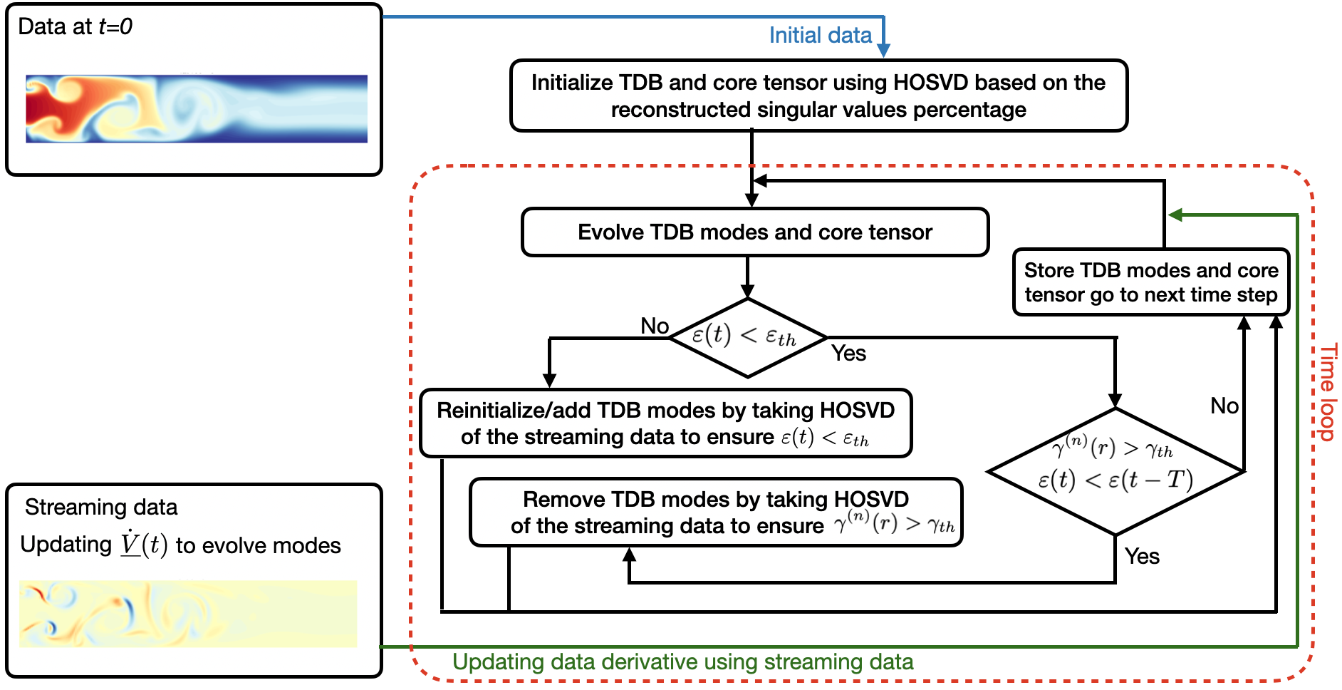
In order to control the error, we define a maximum allowable error for $\varepsilon(t)$, which is chosen by the practitioner. The adaptive algorithm adds modes if the error exceeds the threshold value and removes modes if the error can be maintained below the threshold with lower ranks based on the defined $\gamma^{(n)}(r)$. In particular, if the error exceeds the maximum error ($\varepsilon_{th}$), the algorithm: (i) reinitializes the core tensor and TDB; (ii) increases the number of modes if the resulting error from reinitialization stays above the limit; (iii) the algorithm reinitializes and reduces the number of modes if the solution starts to capture unnecessary energy and has a negative average slope for a defined number of iterations. In this process, we can increase/decrease the number of modes with respect to the relation between the defined error and singular values Eq. (2.21). For example, assume the maximum error limit is set to be $\varepsilon(t)=\varepsilon_{th}$. First, we initialize the TDB and the core tensor using HOSVD and calculate the required number of modes in each direction based on $\gamma^{(n)}(r)=\gamma_{th}$. During the computation, if $\varepsilon(t)>\varepsilon_{th}$, the algorithm reinitializes the modes. If the resulting error is not less than the prescribed limit, the algorithm increases the number of modes based on $\gamma_{th}$. In the subsequent time steps if $\gamma(t)>\gamma_{th}$, the algorithm decreases the number of modes. Note that, rank adjustment reinitializes the modes and the core tensor, which may reduce the error for only a few iterations. This causes frequent rank adjustment with high computational costs. Therefore, in addition to the defined error, the slope of the error for a defined number of iterations (excluding the time steps with HOSVD reinitialization) must be negative to trigger the rank reduction process. We show the algorithm of this example in figure 2.

We show that the computational complexity of solving the resulting equations linearly scales with the size of the data. Here, for simplicity, we consider ($p=d$), i.e., one-dimensional TDB and $N=N_{1}=N_{2}=\dots=N_{d}$. In this case, the total size of the data is $S=N^{d}$. We also consider the case where the core tensor has equal $n$-ranks, i.e., $r=r_{1}=r_{2}=\dots=r_{d}$. The leading costs of evolving TDB equations are:

1. 1.

   Projection of the time-derivative of the data onto TDB ($\mathbf{U}^{(n)^{T}}\mathbf{\dot{\underline{\mathbf{V}}}}_{(n)}$), which is $\mathcal{O}(rdS)$.

2. 2.

   Computing the pseudoinverse of the unfolded core tensor ($\mathbf{T}^{(n)^{\dagger}}$ ). This requires the computation of $\underline{\mathbf{T}}_{(n)}\underline{\mathbf{T}}_{(n)}^{T}$, which scales with $\mathcal{O}(r^{d})$ and the computation of the inverse of this matrix $(\underline{\mathbf{T}}_{1}\underline{\mathbf{T}}_{1}^{T})^{-1})$, which scales with $\mathcal{O}(r^{3})$.

We make the following observations about the cost of evolving TDB:

1. 1.

   When $r<<N$, the computational cost of computing the pseudoinverse of the unfolded core tensor is negligible to the projection of the time-derivative of the data onto TDB, which scales linearly with the total size of the data.

2. 2.

   The evolution of TDB components does not require computation of any eigenvalue problem as required in SVD-based reductions or solving a nonlinear optimization problem as is required in autoencoder-decoder reductions liu2021high, glaws2020deep, mishra2020wavelet.

3. 3.

   Many entries of $\dot{\underline{\mathbf{V}}}$ have small values. See figure 2 for an example of $\dot{\underline{\mathbf{V}}}$. Therefore, the sparse approximation of $\dot{\underline{\mathbf{V}}}$ can significantly reduce overall cost, although this advantage of TDB has not been explored in this work.

The computational cost of solving the TDB equations can be compared against that of computing HOSVD. HOSVD requires computing the SVDs of the unfolded tensor $\underline{\mathbf{V}}_{(n)}$ for $n=1,2,\dots,d$. This requires computation and storage of the correlation matrix $\mathbf{C}^{(n)}=\underline{\mathbf{V}}_{(n)}^{T}\underline{\mathbf{V}}_{(n)}$, which scales with $\mathcal{O}(dN^{d+1})$ and the eigenvalue computation of this matrix, which scales with $N^{3}$. The computational cost of TDB and HOSVD for a block of data generated by the turbulent channel flow simulation (last demonstration) for the case of $N=N_{1}=N_{2}=N_{3}$ are shown in figure 3. This confirms that the computational cost of TDB scales linearly with the total data size $S=N^{3}$, while the computational cost of HOSVD scales with $N^{3}=S^{4/3}$. This shows that TDB computations are significantly faster than HOSVD and the disparity between the computational cost of TDB and HOSVD only grows as the dimension or number of grid points (or samples) increases.

The compression ratio of the TDB decomposition is computed as the ratio of the storage cost of storing the full-dimensional data to that of solving the TDB components. The TDB requires storing the core tensor and the orthonormal lower-dimensional bases. Therefore, the compression ratio for TDB is:

Figure 3 shows the compression ratio ($CR$) for the same problem with the corresponding error resulting from dimension reduction. Since our algorithm is adaptive, it can change the compression ratio by changing the number of modes; therefore, we introduce the weighted compression ratio $\overline{CR}$ as follow:

Where, $CR_{1},CR_{2},\dots CR_{m}$ are compression ratios for $(t_{1}-t_{0}),(t_{2}-t_{1}),\dots,(t_{m}-t_{m-1})$ time intervals, respectively. This equation allows us to measure the effective compression ratio for all time intervals when the number of modes changes in adaptivity process.

We first demonstrate the adaptive TDB compression technique with one dimensional modes (i.e., $d=p$) for a time dependent Runge function as follow:

where $a(t)=1-0.5\exp(-\alpha(t-1)^2)$ and $\alpha=0.5$. For this choice of $a(t)$, the rank of the TDB decomposition must increase from $t=0$ to $t=1$ and then decrease to ensure that the low-rank approximation error remains below a specified value. The spatial domain is the cube $[-\pi,\pi]^{3}$ discretized on a uniform grid of size $126^{3}$. The time step $\Delta t=5\times 10^{-3}$ is used for evolving the TDB evolution equations.

In this problem, we use the same number of modes in each direction, i.e., $r=r_{1}=r_{2}=r_{3}$ due to the isotropy of function $f$. First, we show the effect of both unresolved and numerical errors in figure 4. Here, HOSVD error is the weighted Frobenius norm of the difference between reconstructed data from HOSVD and the streaming data, which shows the unresolved error from reduction. The implemented first-order Euler (EE) and second-order Runge-Kutta (RK) add numerical error to the existing unresolved error. The second-order RK scheme has less error and we use this scheme to show adaptivity effect. This figure also shows the error difference between the exact data derivative with its first-order, and central second-order approximation. In order to study the adaptivity procedure for this analytical problem, we used the data derivative instead of finite difference approximations. Figure 4 shows the reconstruction error versus time for fixed-rank TDB decompositions for $r=2$ and $r=3$ and adaptive TDB initiated with $r=3$. The error threshold and the captured energy percentage is set by practitioner to be $\varepsilon_{th}=10^{-6}$ and $\gamma_{th}=99.999\%$, respectively. It is evident that errors of the fixed-rank approximations $r=2$ and $r=3$ exceed the upper limit of the $10^{-6}$, while the adaptive TDB maintain the error below the upper limit by increasing the rank to $r=4$. The number of modes is later reduced to $r=3$ as the dimensionality of the problem decreases for the given $\gamma_{th}$. Figure 4 shows the singular values of the unfolded core tensor in the $x_{1}$-direction for the fixed-rank and adaptive-rank cases as well as the corresponding HOSVD singular values, which are obtained by taking instantaneous SVD on the unfolded full-dimensional data. This shows that the fixed-rank and adaptive TDB decompositions closely follow the HOSVD.

In the second demonstration, we apply the TDB compression to a turbulent reactive flow. Turbulent reactive flows are multiscale and multivariate, whose high-fidelity numerical simulations result in massive datasets that with the current I/O restrictions of exascale simulations even storing the temporally resolved solution is becoming increasingly challenging let alone probing and analysis of the simulation data. This is particularly the case when a large number of species is involved. An example is the direct numerical simulation (DNS) of turbulent combustion, in which the creation of an ignition kernel – an intermittent phenomenon – occurs on the order of 10 simulation time steps, while typically every 400th time step is stored to maintain the I/O overhead at a reasonable level BAB12. To demonstrate the application of TDB, we consider streaming data generated by a 2D advection-diffusion reaction problem:

where, $\phi_{i}$ is the concentration of $i$th reactant, $\alpha_{i}$ is the associated diffusion coefficient, $Q_{i}^{S}$ denotes the nonlinear source that determines whether $\phi_{i}$ is produced or consumed and $u$ is the velocity field of the flow. The reaction mechanisms model the blood coagulation cascade in a Newtonian fluid LYTK15. The simulation setup chosen in this work is identical to the case considered in reference RNB21. Equation (3.2) is solved for $n_{s}=23$ species and the velocity field is obtained by solving incompressible Navier-Stokes equations at Re=1000 using spectral element discretization. Equation (3.2) is advanced in time using fourth-order RK with $\Delta t=5\times 10^{-4}$. The numerical solution of Eq. (3.2) is cast as a streaming third-order tensor of size $N_{1}\times N_{2}\times N_{3}$, where $N_{1}=251$, $N_{2}=76$ and $N_{3}=n_{3}=23$ are the number of species.

We consider two different TDB compression schemes as follow:

where the inner product in the physical and composition space are as follow:

In TDB-1, $\mathbf{W}^{(1)}$ and $\mathbf{W}^{(2)}$ are quadrature weights obtained from spectral element discretizations of $x_{1}$ and $x_{2}$ directions, respectively. In TDB-2, $\mathbf{W}^{(1)}$ are the quadrature weights for 2D spectral element discretization i.e., both $x_{1}$ and $x_{2}$ directions. The inner product weight in the composition space for both schemes is the identity matrix. The above two schemes have different reduction errors and compression ratios. The main difference between the two decompositions is that in Eq. 3.3, the correlations between both spatial directions, i.e., $x_{1}$, $x_{2}$ and the composition space, i.e., $\eta$ are extracted, whereas in TDB-2, the correlation between $x_{1}$ and $x_{2}$ directions are not extracted. Both schemes are adaptive: modes are added and removed to keep the reconstruction error below $\varepsilon_{th}=10^{-5}$ and the captured details above the $\gamma_{th}=99.999\%$. TDB-2 was recently introduced in Ref. RNB21, where it was referred to as dynamically bi-orthonormal (DBO) decomposition since the species are decomposed to two sets of orthonormal modes in the spatial domain and the composition space. In the DBO formulation presented in Ref. RNB21, full-dimensional Eq. 3.2 is not solved; instead closed-form evolution equations for all three components of TDB-2 are derived, i.e., ODEs for $\underline{\mathbf{T}}_{i_{1}i_{2}}(t)$ and $u^{(2)}_{i_{2}}(\eta,t)$ and PDEs for $u^{(1)}_{i_{1}}(x_{1},x_{2},t)$. We refer to DBO reduction in Ref. RNB21, as model-driven analogue of the data-driven reduction technique presented in this paper, because in the DBO formulation in Ref. RNB21 data generation is not required. In this section, we compare the model-driven DBO bases and the data-driven DBO bases that are the focus of this paper.

References

- [1] J. Slotnick, A. Khodadoust, J. Alonso, D. Darmofal, W. Gropp, E. Lurie, and D. Mavriplis, “CFD vision 2030 study: a path to revolutionary computational aerosciences,” National Aeronautics and Space Administration, Langley Research Center, 2014.
- [2] E. P. Duque, S. T. Imlay, S. Ahern, C. Guoning, and D. L. Kao, “Nasa cfd vision 2030 visualization and knowledge extraction: Panel summary from aiaa aviation 2015 conference,” in 54th AIAA Aerospace Sciences Meeting, p. 1927, 2016.
- [3] J. Dongarra, J. Hittinger, J. Bell, L. Chacon, R. Falgout, M. Heroux, P. Hovland, E. Ng, C. Webster, and S. Wild, “Applied mathematics research for exascale computing,” tech. rep., Lawrence Livermore National Lab.(LLNL), Livermore, CA (United States), 2014.
- [4] “Data reduction for science,” Report of the DOE Workshop on Brochure from Advanced Scientific Computing Research Workshop, 2021.
- [5] J. C. Bennett, H. Abbasi, P. Bremer, R. Grout, A. Gyulassy, T. Jin, S. Klasky, H. Kolla, M. Parashar, V. Pascucci, P. Pebay, D. Thompson, H. Yu, F. Zhang, and J. Chen, “Combining in-situ and in-transit processing to enable extreme-scale scientific analysis,” in SC ’12: Proceedings of the International Conference on High Performance Computing, Networking, Storage and Analysis, pp. 1–9, 2012.
- [6] S. W. Son, Z. Chen, W. Hendrix, A. Agrawal, W.-k. Liao, and A. Choudhary, “Data compression for the exascale computing era-survey,” Supercomputing frontiers and innovations, vol. 1, no. 2, pp. 76–88, 2014.
- [7] S. Li, N. Marsaglia, C. Garth, J. Woodring, J. Clyne, and H. Childs, “Data reduction techniques for simulation, visualization and data analysis,” in Computer Graphics Forum, vol. 37, pp. 422–447, Wiley Online Library, 2018.
- [8] P. Lindstrom and M. Isenburg, “Fast and efficient compression of floating-point data,” IEEE transactions on visualization and computer graphics, vol. 12, no. 5, pp. 1245–1250, 2006.
- [9] N. Fout and K.-L. Ma, “An adaptive prediction-based approach to lossless compression of floating-point volume data,” IEEE Transactions on Visualization and Computer Graphics, vol. 18, no. 12, pp. 2295–2304, 2012.
- [10] H. Cheng, Z. Gimbutas, P.-G. Martinsson, and V. Rokhlin, “On the compression of low rank matrices,” SIAM Journal on Scientific Computing, vol. 26, no. 4, pp. 1389–1404, 2005.
- [11] A. M. Dunton, L. Jofre, G. Iaccarino, and A. Doostan, “Pass-efficient methods for compression of high-dimensional turbulent flow data,” Journal of Computational Physics, vol. 423, p. 109704, 2020.
- [12] C. W. Therrien, Discrete random signals and statistical signal processing. Prentice Hall PTR, 1992.
- [13] J. A. Tropp, A. Yurtsever, M. Udell, and V. Cevher, “Practical sketching algorithms for low-rank matrix approximation,” SIAM Journal on Matrix Analysis and Applications, vol. 38, no. 4, pp. 1454–1485, 2017.
- [14] H. Kolla, K. Aditya, and J. H. Chen, Higher Order Tensors for DNS Data Analysis and Compression, pp. 109–134. Cham: Springer International Publishing, 2020.
- [15] G. Zhou, A. Cichocki, and S. Xie, “Decomposition of big tensors with low multilinear rank,” 2014.
- [16] K. T. Carlberg, A. Jameson, M. J. Kochenderfer, J. Morton, L. Peng, and F. D. Witherden, “Recovering missing cfd data for high-order discretizations using deep neural networks and dynamics learning,” Journal of Computational Physics, vol. 395, pp. 105–124, 2019.
- [17] A. Glaws, R. King, and M. Sprague, “Deep learning for in situ data compression of large turbulent flow simulations,” Physical Review Fluids, vol. 5, no. 11, p. 114602, 2020.
- [18] Y. Liu, Y. Wang, L. Deng, F. Wang, F. Liu, Y. Lu, and S. Li, “A novel in situ compression method for cfd data based on generative adversarial network,” Journal of Visualization, vol. 22, no. 1, pp. 95–108, 2019.
- [19] Z. Gong, T. Rogers, J. Jenkins, H. Kolla, S. Ethier, J. Chen, R. Ross, S. Klasky, and N. F. Samatova, “Mloc: Multi-level layout optimization framework for compressed scientific data exploration with heterogeneous access patterns,” in 2012 41st International Conference on Parallel Processing, pp. 239–248, IEEE, 2012.
- [20] T. P. Sapsis and P. F. Lermusiaux, “Dynamically orthogonal field equations for continuous stochastic dynamical systems,” Physica D: Nonlinear Phenomena, vol. 238, no. 23-24, pp. 2347–2360, 2009.
- [21] M. Cheng, T. Y. Hou, and Z. Zhang, “A dynamically bi-orthogonal method for time-dependent stochastic partial differential equations i: Derivation and algorithms,” Journal of Computational Physics, vol. 242, pp. 843–868, 2013.
- [22] M. Choi, T. P. Sapsis, and G. E. Karniadakis, “On the equivalence of dynamically orthogonal and bi-orthogonal methods: Theory and numerical simulations,” Journal of Computational Physics, vol. 270, pp. 1 – 20, 2014.
- [23] E. Musharbash and F. Nobile, “Dual dynamically orthogonal approximation of incompressible N]avier [Stokes equations with random boundary conditions,” Journal of Computational Physics, vol. 354, pp. 135–162, 2018.
- [24] H. Babaee, “An observation-driven time-dependent basis for a reduced description of transient stochastic systems,” Proceedings of the Royal Society A: Mathematical, Physical and Engineering Sciences, vol. 475, no. 2231, p. 20190506, 2019.
- [25] P. Patil and H. Babaee, “Real-time reduced-order modeling of stochastic partial differential equations via time-dependent subspaces,” Journal of Computational Physics, vol. 415, p. 109511, 2020.
- [26] H. Babaee and T. Sapsis, “A minimization principle for the description of modes associated with finite-time instabilities,” Proceedings of the Royal Society A: Mathematical, Physical and Engineering Sciences, vol. 472, no. 2186, p. 20150779, 2016.
- [27] A. Blanchard, S. Mowlavi, and T. Sapsis, “Control of linear instabilities by dynamically consistent order reduction on optimally time-dependent modes,” Nonlinear Dynamics, vol. In press, 2018.
- [28] M. Donello, M. Carpenter, and H. Babaee, “Computing sensitivities in evolutionary systems: A real-time reduced order modeling strategy,” arXiv preprint arXiv:2012.14028, 2020.
- [29] A. G. Nouri, H. Babaee, P. Givi, H. K. Chelliah, and D. Livescu, “Skeletal model reduction with forced optimally time dependent modes,” Combustion and Flame, p. 111684, 2021.
- [30] M. H. Beck, A. Jäckle, G. A. Worth, and H. D. Meyer, “The multiconfiguration time-dependent Hartree (MCTDH) method: a highly efficient algorithm for propagating wavepackets,” Physics Reports, vol. 324, pp. 1–105, 1 2000.
- [31] C. Bardos, F. Golse, A. D. Gottlieb, and N. J. Mauser, “Mean field dynamics of fermions and the time-dependent Hartree–Fock equation,” Journal de Mathématiques Pures et Appliquées, vol. 82, no. 6, pp. 665–683, 2003.
- [32] O. Koch and C. Lubich, “Dynamical tensor approximation,” SIAM Journal on Matrix Analysis and Applications, vol. 31, pp. 2360–2375, 2017/04/02 2010.
- [33] A. Dektor and D. Venturi, “Dynamically orthogonal tensor methods for high-dimensional nonlinear pdes,” Journal of Computational Physics, vol. 404, p. 109125, 2020.
- [34] T. G. Kolda and B. W. Bader, “Tensor decompositions and applications,” SIAM Review, vol. 51, no. 3, pp. 455–500, 2009.
- [35] D. Ramezanian, A. G. Nouri, and H. Babaee, “On-the-fly reduced order modeling of passive and reactive species via time-dependent manifolds,” Computer Methods in Applied Mechanics and Engineering, vol. 382, p. 113882, 2021.
- [36] T. Sapsis and P. Lermusiaux, “Dynamically orthogonal field equations for continuous stochastic dynamical systems,” Physica D: Nonlinear Phenomena, vol. 238, no. 23-24, pp. 2347–2360, 2009.
- [37] H. Babaee and T. P. Sapsis, “A minimization principle for the description of modes associated with finite-time instabilities,” Proceedings of the Royal Society of London A: Mathematical, Physical and Engineering Sciences, vol. 472, no. 2186, 2016.
- [38] M. Cheng, T. Y. Hou, and Z. Zhang, “A dynamically bi-orthogonal method for time-dependent stochastic partial differential equations i: Derivation and algorithms,” Journal of Computational Physics, vol. 242, no. 0, pp. 843 – 868, 2013.
- [39] H. Babaee, M. Farazmand, G. Haller, and T. P. Sapsis, “Reduced-order description of transient instabilities and computation of finite-time Lyapunov exponents,” Chaos: An Interdisciplinary Journal of Nonlinear Science, vol. 27, p. 063103, 06 2017.
- [40] A. J. Chorin, O. H. Hald, and R. Kupferman, “Optimal prediction and the mori–zwanzig representation of irreversible processes,” Proceedings of the National Academy of Sciences, vol. 97, no. 7, pp. 2968–2973, 2000.
- [41] T. Liu, J. Wang, Q. Liu, S. Alibhai, T. Lu, and X. He, “High-ratio lossy compression: Exploring the autoencoder to compress scientific data,” IEEE Transactions on Big Data, 2021.
- [42] D. Mishra, S. K. Singh, and R. K. Singh, “Wavelet-based deep auto encoder-decoder (wdaed)-based image compression,” IEEE Transactions on Circuits and Systems for Video Technology, vol. 31, no. 4, pp. 1452–1462, 2020.
- [43] Z. Li, A. Yazdani, A. Tartakovsky, and G. E. Karniadakis, “Transport dissipative particle dynamics model for mesoscopic advection-diffusion-reaction problems,” The Journal of Chemical Physics, vol. 143, p. 014101, 2020/07/13 2015.
- [44] K. Braman, T. A. Oliver, and V. Raman, “Adjoint-based sensitivity analysis of flames,” Combustion Theory and Modelling, vol. 19, pp. 29–56, 01 2015.
- [45] M. Lemke, L. Cai, J. Reiss, H. Pitsch, and J. Sesterhenn, “Adjoint-based sensitivity analysis of quantities of interest of complex combustion models,” Combustion Theory and Modelling, vol. 23, pp. 180–196, 01 2019.
- [46] R. Langer, J. Lotz, L. Cai, F. vom Lehn, K. Leppkes, U. Naumann, and H. Pitsch, “Adjoint sensitivity analysis of kinetic, thermochemical, and transport data of nitrogen and ammonia chemistry,” Proceedings of the Combustion Institute, 2020.
- [47] V. Vuorinen and K. Keskinen, “Dnslab: A gateway to turbulent flow simulation in matlab,” Computer Physics Communications, vol. 203, pp. 278–289, 2016.