Vibrational tunneling spectra of molecules with asymmetric wells: a combined vibrational configuration interaction and instanton approach
Abstract
A combined approach that uses the vibrational configuration interaction (VCI) and semiclassical instanton theory was developed to study vibrational tunneling spectra of molecules with multiple wells in full dimensionality. The method can be applied to calculate low-lying vibrational states in the systems with arbitrary number of minima, which are not necessarily equal in energy or shape. It was tested on a two-dimensional double-well model system and on malonaldehyde and the calculations reproduced the exact quantum-mechanical results with high accuracy. The method was subsequently applied to calculate vibrational spectrum of the asymmetrically deuterated malonaldehyde with non-degenerate vibrational frequencies in the two wells. The spectrum is obtained at a cost of single-well VCI calculations used to calculate the local energies. The interactions between states of different wells are computed semiclassically using instanton theory at a comparatively negligible computational cost. The method is particularly suited to systems in which the wells are separated by large potential barriers and tunneling splittings are small, e.g, in some water clusters, when the exact quantum-mechanical methods come at a prohibitive computational cost.
I Introduction
Physical systems with multiple energetically stable minima are ubiquitous in chemistry and physics Bell 1980. Bound states that are localized in such wells, separated by potential barriers, interact via quantum tunneling, which results in observable shifts of their energies Hund 1927; Benderskii, Makarov, and Wight 1994. For equivalent, symmetry-related wells, the states that would be degenerate in the absence of tunneling, produce a splitting pattern of energy levels.
Molecules and molecular complexes with two or more equivalent stable configurations are multidimensional systems that display these effects in their vibrational spectrum. The inversion of ammonia Urban et al. 1981, proton tunneling in malonaldehyde Firth et al. 1991, double proton transfer in porphycene Mengesha et al. 2013 or bond rotation in vinyl radical Tanaka et al. 2004 are examples of symmetric double-well systems that produce measurable tunneling splittings (TS) of their vibrational state energies. Water clusters are prototype multiwell systems that exhibit nontrivial splitting patterns caused by tunneling rearrangements between many stable configurations of the cluster Cvitaš and Richardson 2020.
The asymmetric systems, which have non-equivalent wells, have been less studied. When the state energies of different wells are in resonance, the tunneling dynamics will again cause the delocalization of the wavefunction across the wells and the energy shifts in the spectrum Benderskii, Makarov, and Wight 1994. Away from the resonance, the states remain localized in one well. The asymmetry can be induced in symmetric molecular systems by asymmetric isotopic substitutions Jahr, Laude, and Richardson 2020. The normal modes and vibrational frequencies in equivalent symmetry-related potential wells then differ and the correspondence of the vibrational wavefunctions of different wells is not preserved in general. As an example, the malonaldehyde molecule deuterated at D7/D9 position (see Figure 3) thus has an asymmetric level structure with the localized states and those that are delocalized across the multiple minima Jahr, Laude, and Richardson 2020. A mixing angle between the left-right ground vibrational states of partially deuterated malonaldehyde has been determined experimentally Baughcum et al. 1981. Further examples of the mixing have been studied in HFHD dimer Zhang et al. 1995 and partially deuterated vinyl radical Šmydke et al. 2019, CHDCH, using full-dimensional exact calculations. The splitting pattern in partially deuterated water trimers HDO(H2O)2 and D2O(H2O)2 have been determined in experiment Liu et al. 1996 and by us using instanton theory Eraković and Cvitaš 2021.
The asymmetry in molecules can also be found in some tautomers. In this case, potential energy surface (PES) does not possess a symmetry relating the wells and their shapes, and the minimum energies are different. A possible candidate belonging to this class is 2-hydroxy-1-naphthaldehyde, shown in Figure 1. Hydroxyl proton forms a hydrogen bond with the oxygen atom of the carbonyl group, and can tunnel to it to form a tautomer, which is a local minimum.

Thiomalonaldeyde has two nearly degenerate minima in the form of enol and enethiol tautomers, shown in Figure 2. Enethiol is about 70 cm-1 more stable González, Mó, and Yáñez 1997, with the barrier height to interconversion slightly lower than in the malonaldehyde. This implies that the TS is similar in magnitude to the energy asymmetry of the wells and the states in different wells that lie below the barrier are expected to interact. Interestingly, it has been suggested González, Mó, and Yáñez 1997 that the replacement of hydrogen, shared by the hydrogen bonds OHS and SHO, by deuterium reverses the stability order of tautomers due to zero-point energy effect.

The asymmetry can also be caused by environment. Molecules in rare gas matrices can have energy asymmetry between the wells comparable to their TS in isolation. Delocalization of the tunneling hydrogen was observed Bondybey, Haddon, and Rentzepis 1984 in 9-hydroxyphenalone embedded in a neon matrix. Molecules in crystals in the vicinity of a suitable guest molecule can also have comparable energies of the splitting and energy asymmetry of the wells Oppenländer et al. 1989.
Quantum tunneling has also been observed in macroscopic systems. Tunneling of Bose-Einstein condensates Hall et al. 2007, electron spin tunneling in the nanomagnetic molecules Takahashi et al. 2011 or the tunneling of magnetic flux in superconducting circuits based on Josephson junctions Johnson et al. 2005 are some recent examples. In a collective macroscopic variable, these processes can be described by a double well with externally controllable parameters that can induce asymmetry between the wells.
Calculation of TS in moderately large molecules is prohibitively costly. Exact variational methods for determining the bound states of molecules scale exponentially with the basis set size while large basis sets are often required Felker and Bačić 2019. Basis functions need to span over two or more wells sufficiently densely to obtain enough resolution to extract the splittings from the difference of the energies in their spectrum. The asymmetry of the wells also suggests that the symmetry cannot be used to reduce the size of the problem. Full-dimensional studies of malonaldehyde using multiconfigurational time-depedent Hartree Schröder and Meyer 2014; Hammer and Manthe 2012 (MCTDH), variational calculations on HF dimer Felker and Bačić 2019 or H2O dimer Leforestier, Szalewicz, and van der Avoird 2012 represent the state-of-the-art calculations of the vibrational levels using formally exact methods.
A direct calculation of TS in larger systems can be performed using a recently developed path integral molecular dynamics method Vaillant, Wales, and Althorpe 2018 based on the potential sampling around the minimum action paths (MAP) connecting different wells. The multi-well splitting patterns of water trimer and hexamer Vaillant, Wales, and Althorpe 2019 were obtained in this way using a matrix model of hamiltonian in the basis of local vibrational states. The tunneling matrix (TM) elements are extracted from the zero-temperature limit of the partition function, which means that the method only works for the vibrational ground-state in symmetric well systems.
Alternatively, the TM elements can be estimated using semiclassical methods. From that class, the instanton method, which comes in several forms Benderskii et al. 1997; Smedarchina, Siebrand, and Fernández-Ramos 2012; Richardson and Althorpe 2011; Mil’nikov and Nakamura 2001, has some particularly appealing features. It can be applied in Cartesian coordinates Richardson and Althorpe 2011; Eraković, Vaillant, and Cvitaš 2020 to any molecule without modification. Numerically, it relies on the optimization of the minimum action path (MAP) that connects the symmetry-related minima Cvitaš and Althorpe 2016, and requires the potential and hessians of the potential along the MAP to evaluate the splittings. It thus relies on a modest number of potential and gradient evaluations Cvitaš 2018 in comparison with the exact quantum-mechanical (QM) methods. This allows one to perform calculations in full dimensionality or in combination with on-the-fly evaluation of the electronic potential. Additionally, its accuracy is higher for large barriers and small splittings. Precisely in this regime, the exact variational methods become inefficient and resource intensive.
The first derivation of multidimensional instanton theory was accomplished by means of Jacobi fields integration (JFI) Mil’nikov and Nakamura 2001. JFI method has been used to determine TSs for a range of symmetric double-well systems, such as malonaldehyde Mil’nikov and Nakamura 2001; Cvitaš and Althorpe 2016; Cvitaš 2018, vinyl radical Mil’nikov, Ishida, and Nakamura 2006, and formic acid dimer Mil’nikov, Kühn, and Nakamura 2005. The instanton method was later rederived in the ring polymer form (RPI) Richardson and Althorpe 2011, which could treat asymmetric potentials along MAPs and multiple wells. The RPI was used to calculate and interpret experimental ground-state splitting patterns of water clusters in terms of their rearrangement dynamics Cvitaš and Richardson 2020 for the dimer, Richardson and Althorpe 2011; Vaillant and Cvitaš 2018; Zwart et al. 1991 trimer Richardson and Althorpe 2011; Keutsch, Cruzan, and Saykally 2003 hexamer Richardson et al. 2016 and octamer Richardson et al. 2013. We recently generalized the JFI method Eraković, Vaillant, and Cvitaš 2020 to treat the multi-well systems and used it to explain the ground-state splitting pattern of 320 states in the water pentamer in terms of five dominant rearrangement pathways Cvitaš and Richardson 2019. The extension of the method to low-lying vibrational states Eraković and Cvitaš 2020 is based on work of Mil’nikov and Nakamura Mil’nikov and Nakamura 2005 and forms the groundwork of calculating the TM elements between local vibrational states of different wells in the present study below.
Weakly biased double-well systems have been considered in previous work by several authors. Analytical results in one dimension have been obtained using semiclassical WKB and instanton methods. Garg has demonstrated Garg 2000 that the instanton and the WKB method with Herring formula Herring 1962 give equivalent results for TS in symmetric systems. Cesi et al. Cesi, Rossi, and Testa 1991 considered a one-dimensional (1D) double-well with the shape asymmetry and no energy asymmetry using instantons and obtained an expression for the ground-state TS. An approximate solution for a 1D double well with a weak bias was also obtained by Mugnai and Ranfagni Mugnai and Ranfagni 1985, using instantons based on the MAP that does not fully connect the minima of the two wells. Leggett et al obtained a solution Leggett et al. 1987 by adding a parabolic correction potential to remove the asymmetry between the wells, the contribution of which was then subsequently subtracted from the action integral. Dekker Dekker 1987 derived the ground-state TS from the quantization condition by asymptotic matching of the semiclassical wavefunction in the barrier to the parabolic cylinder wavefunctions of harmonic oscillators in the two wells. Song Song 2008; Song 2015 extended Dekker’s method Dekker 1987 (as have Halataie and Leggett Halataei and Leggett 2017 done independently) to obtain the TS in vibrationally excited states of asymmetric 1D potentials with arbitrarily large shape and energy asymmetry. Song also showed Song 2015 that the instanton wavefunctions with the Herring formula in a matrix model give equivalent results to those obtained by Dekker’s method Dekker 1987.
In multidimensional systems, tunneling can be assisted or supressed by the excitation of transversal vibrational modes Mil’nikov and Nakamura 2005; Siebrand, Smedarchina, and Fernández-Ramos 2013. In the presence of asymmetry, the excited states of one well can be in a resonance with the states of another well with a different set of local quantum numbers, which results in a delocalization of the wavefunction across these wells Song 2015. Benderskii et al devised a multidimensional perturbative instanton method Benderskii, Vetoshkin, and Trommsdorff 1999 in which they treat the asymmetry of the potential in an analytic two-dimensional model as a correction of first order in , same as energy. In this way, the MAP remains symmetric and the asymmetry is moved to the transport equation along with energy. They also show that the equivalent expressions for the TS are obtained using the instanton quantization condition of Dekker Dekker 1987 and using the instanton or WKB wavefunctions with Herring formula Herring 1962 in 1D. The method was applied to calculate TSs in excited vibrational states of malonaldehyde Benderskii et al. 2000 with the asymmetric isotopic substitutions using a fit of model potential parameters to quantum-chemical data. The extensions of the RPI and JFI method to the ground-states of the asymmetric systems with a weak bias have recently been derived and applied to partially deuterated malonaldehyde Jahr, Laude, and Richardson 2020 and water trimer Eraković and Cvitaš 2021, respectively.
The object of this paper is to propose a method for calculating vibrational tunneling spectrum of multi-well systems of mid-sized molecules that are outside reach of the exact quantum methods. For this purpose, we extend the usual matrix model to the model, which represents the molecular Hamiltonian in the basis of all local vibrational states of each well . We rederive a generalized Herring formula Herring 1962; Benderskii, Vetoshkin, and Trommsdorff 1999 in order to calculate the off-diagonal TM elements that represent the interaction of local vibrational states of different wells. The semiclassical wavefunctions at the dividing plane, in the barrier that separates the wells, are obtained using the recently generalized JFI method Mil’nikov and Nakamura 2005; Eraković, Vaillant, and Cvitaš 2020. The JFI wavefunctions are thus used to calculate the couplings between states that have different energies and normal-mode excitations for the first time. The diagonal energies of the local vibrational states can be calculated using any accurate quantum method with a basis set that spans only one well. Vibrational configuration interaction Carter, Bowman, and Handy 1998; Christoffel and Bowman 1982; Bowman, Christoffel, and Tobin 1979 (VCI) is used in this work. The effect of rotations is neglected.
The method, presented in Section II, allows one to study vibrational structure in asymmetric systems with multiple wells, separated by large potential barriers, in an approximate manner. The accuracy of the method is tested on a two-dimensional double-well model in Section III A. In Section III B, it is applied to the (symmetric) malonaldehyde molecule, which tests the accuracy of the matrix model using a combination of VCI and JFI matrix elements on a realistic PES, in vibrationally excited states, against the exact MCTDH calculations. Vibrational tunneling spectrum of the partially deuterated malonaldehyde is calculated in Section III C, which features the mixing of inequivalent well states due to tunneling. The paper concludes in Section IV.
II TUNNELING MATRIX
Without the loss of generality, we start by considering a system with two minima separated by a large potential barrier. The minima, denoted as ‘left’ (L) and ‘right’ (R), are not necessarily symmetric either in shape or energy. For low-energy spectra, the vibrational Hamiltonian can be represented in the basis of states that are localized in the wells, , as
| (1) |
Square blocks are formed using basis functions of the same minimum and are not necessarily of equal size. Their off-diagonal elements describe the interaction between different basis functions localized in the same minimum and can be made small by a suitable choice of the basis. In the instanton theory of tunneling splittings, the usual presumption is that the local vibrational wavefunctions are harmonic oscillator states. In that case, the off-diagonal terms describe anharmonic contributions that originate from the difference between the actual and the harmonic potential.
In our approach here, we replace the harmonic surface of each well by an -mode representation Bowman, Carter, and Huang 2003; Rauhut 2004 of the well potential and calculate local eigenfunctions and eigenvalues using vibrational self consisten field (VSCF) and vibrational configuration interaction (VCI) methods Carter, Bowman, and Handy 1998; Christoffel and Bowman 1982; Bowman, Christoffel, and Tobin 1979. The technical details of the calculations are described in Appendix C. Using the more accurate local wavefunctions as a basis reduces the magnitude of the off-diagonal matrix elements in , which we then neglect. The matrices become diagonal and the diagonal matrix elements are referred to as the local vibrational energies of the left/right (L/R) well. For symmetric wells, the local energies are doubly degenerate.
The block in matrix (1) contains the TM elements that describe the interaction of local wavefunctions of the left and right minimum. The exact quantal calculation of these elements requires a large basis set that can accurately represent the form of the wavefunction inside the barrier. Instead, we obtain them by means of Herring formula Herring 1962 in combination with the semiclassical wavefunctions from the instanton theory Mil’nikov and Nakamura 2005; Eraković and Cvitaš 2020. Since the only effect of matrix (1) is to mix local wavefunctions of different minima via tunneling, we refer to it as the tunneling matrix Richardson and Althorpe 2011.
We now derive the Herring formula without the usual assumptions of the two-state model and the L/R symmetry. Rather, we consider Schrödinger equation with Hamiltonian (or tunneling) matrix (1) from which it follows that
| (2) |
where are the local vibrational energies and the summation over repeated indices is assumed. Next, a dividing plane is defined inside the barrier via the implicit equation , which separates the left from the right minimum. Eqns. (2) are multiplied by and , respectively, subtracted and integrated over the left part of the domain (i.e., over the space on the ‘left’ side of the dividing plane). The local wavefunctions , either harmonic or VCI, have been obtained as eigenfunctions of a hermitian matrix and are therefore taken to be orthonormal. For a sufficiently high barrier, the wavefunctions can be considered small in the R/L domain, respectively. We thus neglect the integrals involving the like products in the L volume and extend the integrals involving over the entire domain to produce . The integrals involving the mixed products have also been neglected. The error introduced by the neglect of these terms outside the resonance, i.e., for , is analysed in Appendix B. The TM element is then expressed as
| (3) |
where, in the last step, we use the divergence theorem to turn the spatial integration into the integral over the dividing plane. in Eq. (3) denotes the coordinate that describes an orthogonal shift from the dividing plane.
Local wavefunctions, that we designed to calculate the local vibrational energies on the diagonal of matrix (1), are constructed using VSCF/VCI on an approximate PES (see Appendix C) and their accuracy drops inside the barrier that separates the wells. In order to evaluate the surface integral in Herring formula, Eq. (3), inside the barrier, we employ the JFI wavefunctions instead, which we recently derived in Ref. Eraković and Cvitaš 2020. These are based on the WKB method in which the energy is treated as a term of order and is moved to the transport equation, leaving the Hamilton-Jacobi equation energy independent. It was shown that this approach gives equivalent results to the standard WKB method in 1D Garg 2000. Moreover, the ground-state TS obtained from Herring formula using the ground-state JFI wavefunctions Eraković and Cvitaš 2020 is identical to the standard instanton result derived from the steepest descent approximation of the partition function in the path integral formulation Eraković, Vaillant, and Cvitaš 2020.
The characteristic of the Hamilton-Jacobi equation that connects the minimum of a well to a point in configuration space obeys the equation Eraković and Cvitaš 2020
| (4) |
and represents a classical trajectory on the inverted PES, parametrized by the ‘imaginary’ time . In order to represent the quantities in the neighborhood of the characteristic, local coordinates are defined Mil’nikov and Nakamura 2005; Eraković and Cvitaš 2020, where is the mass-scaled arc length distance from the minimum along the characteristic and is the orthogonal shift from the nearest point on the characteristic. The classical momentum is defined as
| (5) |
and can be used, instead of , to reparametrize the characteristic. Local wavefunctions in the harmonic vicinity of the characteristic are obtained by integrating the Hamilton-Jacobi and transport equations on the characteristic Eraković and Cvitaš 2020 as
| (6) |
For vibrationally excited states, the label in Eq. (6) is the number of quanta in the excited vibrational mode of frequency . Matrices are Gaussian widths of the wavefunction in the directions orthogonal to the characteristic and are obtained from
| (7) |
in Eq. (7) is Hessian of the potential at , which is used to approximate the potential up to quadratic terms in the neighborhood of the characteristic. The initial condition for Eq. (7) at the minimum is , where is Hessian at the L/R minimum. For vibrationally excited states, the prefactor in the parenthesis in Eq. (6) contains terms and , which are defined via equations
| (8) |
terms account for the change in the amplitude of the excited-state wavefunction along the characteristic, while the term describes the nodal plane. The initial condition for is found by matching the instanton wavefunction to that of the harmonic oscillator at a small distance from the minimum, as . The is the excited-state normal mode, i.e., the eigenvector of having frequency , and serves as the initial condition for in Eq. (8).
The local instanton wavefunctions, Eq. (6), for the left and right minimum are next inserted into Herring formula Eq. (3), without the previous assumption Eraković and Cvitaš 2020 that and refer to the excitation of the same normal mode and the same number of quanta . For that purpose, a connection point is chosen on the dividing surface inside the barrier and characteristics determined, which connect it to the minima on both sides of the dividing surface. The shape of the characteristic between two points in configuration space is determined by minimizing the Jacobi action Cvitaš and Althorpe 2016. The surface integral in Eq. (3) can then be computed analytically Eraković and Cvitaš 2020.
This approach yields best results if the connection point is chosen so that both wavefunctions are near their maxima in the dividing plane at the connection point. This can be obtained by minimization of the sum of action integrals . For minima of the same energy, this procedure yields the minimum action path (MAP) that connects the minima and any point on that path is a suitable candidate for the connection point. The dividing surface can then be chosen as the plane orthogonal to the MAP at the connection point. If the minima do not have the same energies, but differ by the amount , this procedure is equivalent to determining the MAP on the modified PES , where is the position of the connection point on the characteristic and is the Heaviside step function. In this case, the position of the connection point has to be given a priori, and the resulting path will depend on its position. The safest choice is to pick the connection point in the middle of the MAP, which is expected to be near the maximum of the potential energy barrier. For minima at different energies, the resulting MAP is going to have a tangent dicontinuity at the connection point as at . The tangent direction at the connection point is then defined as the average tangent of its L and R limit at . Again, the dividing plane is taken to be orthogonal to the MAP and the surface integral in Eq. (3) is solved analytically. The TM element then becomes
| (9) |
with all quantities in the brackets evaluated at . In Eq. (9), is the total length of the MAP, and the symbol means that the tangent direction to the MAP was explicitly projected out. det’ in Eq. (9) denotes the product of all non-zero eigenvalues. Matrices have zero eigenvalues associated with the overal translations and rotations, while has an additional zero eigenvalue associated with the tangent to the MAP. For energy-equivalent minima, the tangent vector is an eigenvector of with zero eigenvalue and the explicit projection to the orthogonal space is not needed. The TM element in Eq. (9) is valid for , . For and multiple excitations in different modes, the TM element can still be evaluated using Herring formula and wavefunctions of form (6) using analytical integrals, but we have only implemented it numerically, without trying to write down the explicit form. We also remark here that the wavefunction in Eq. (6) for the multiply excited normal modes, , does not correspond to the harmonic oscillator wavefunction near the minimum, as the prefactor in Eq. (6) is not a Hermite polynomial. We further note that the TM element, (9), is not invariant with respect to the position of the connection point unless the two local states are in resonance, as shown in Appendix B.
III NUMERICAL TESTS
Numerical tests were carried out on a model two-dimensional (2D) PES and on malonaldehyde molecule with some atoms substituted with heavier isotopes. MAPs that connect the minima were determined using the string method Cvitaš and Althorpe 2016; Cvitaš 2018. The criterion for convergence was chosen to be the largest component of gradient of Jacobi action perpendicular to the path and was set to . Number of beads used to discretize the string was 301 for model potential, which is much larger than necessary for convergence, but was used to ensure that all results obtained using different parameters of the potential are sufficiently converged. For potential with minima at different energies, the dividing plane was set to pass through the central bead and perpendicular to the MAP. In the case of malonaldehyde, the number of beads was 201 and the minima were oriented towards the first neighboring bead in each step of the optimization to minimise the root-mean-square distance between their geometries Cvitaš and Althorpe 2016. After optimization, Hessians of the potential were determined at each bead on the MAP. Translations and rotations were explicitly projected out from Hessians Eraković, Vaillant, and Cvitaš 2020. Geometries along the path in mass-scaled Cartesian coordinates, potential and Hessian matrix elements were parametrized by the arc length along the MAP and interpolated using natural cubic splines. Matrices in Eq. (7) were propagated using the previously described approach Eraković and Cvitaš 2020, with the initial ‘jump’ at for model potential and for malonaldehyde. Fourth order Runge-Kutta method was used for integration of Eq. (7). Matrices were saved at each bead and their matrix elements interpolated using natural cubic splines, as for Hessians above. The interpolant was then used to propagate and in Eq. (8) from minima up to the the dividing plane.
The particular implementation of the VSCF/VCI method that is employed in our calculation here is described in Appendix C. We determined the 1-mode and 2-mode terms of the PES and neglected the terms beyond. In each normal mode, the potential was evaluated at Gauss-Hermite discrete-variable-representation (DVR) points, which correspond to the zeroes of Hermite polynomials. We used 8 DVR points for the 2D model potential and 11 DVR points for malonaldehyde. This approach utilizes the natural lengthscales of the harmonic oscillators in each normal mode, which gives a balanced description of potential at different minima. The 1-mode terms were then fitted to the eighth-order polynomials using linear regression. For 2-mode terms, the potential was computed on a rectangular grid of DVR points determined above and a fit was performed analogously. For each 1-mode potential, a quick QM calculation was performed using sine DVR basis with 100 basis functions. The difference in the lowest two energies from that calculation was used as a frequency for the harmonic oscillator basis set, which was used to solve the VSCF equations. This approach provides a better basis for determining the 1-mode potentials which quickly deviate from the harmonic curve, reducing the number of basis functions needed to describe the 1-mode functions in VSCF. and basis functions were used for each normal mode for the 2D model potential and malonaldehyde, respectively, to converge the energies. A larger basis should not be used, as functions corresponding to larger energies penetrate into unphysical part of the fitted potential, which can cause appearance of intruder states and worse energies. After VSCF calculation, the computed 1-mode functions were used for VCISD calculation, where the highest excitation in each mode was limited to 6 in both, the 2D model system and malonaldehyde.
III.1 2D MODEL POTENTIAL
The 2D model potential with two minima, which we use in our test calculations below, is defined by the following equations,
| (10) |
where are not mass scaled. Minima are located at . Coefficients and are chosen so that in the vicinity of left minimum, the potential is approximately harmonic and equals , while in the vicinity of the right minimum, the potential is approximately harmonic and shifted in energy by , i.e., . and are eigenvalues of Hessian, while are normal modes. Parameter denotes the angle of inclination of normal mode to axis. Mass of the system was taken to be in both dimensions, so that the harmonic frequencies are given by .
The above form of the potential can be used to independently vary harmonic frequencies , by changing parameters , or the shift without affecting the other parameters of either the left or the right minimum. In this paper, the parameters of the left minimum were , . The parameters of the right minimum were the same as the parameters of the left, for the symmetric case with . To obtain the asymmetric potentials below, one of the three parameters was varied, with going from to , parameter going from to and going from to . Positions of the minima were set with and the angle . This angle corresponds to approximately equal contributions of and in the TM elements Eraković and Cvitaš 2020. Figure 4 shows the model potential for a selection of parameters , and .
Frequency is the lower frequency and the MAP enters the minima along the corresponding normal mode. Consequently, does not contribute towards the zero-point energy in the plane orthogonal to the MAP. The effective barrier for the tunneling motion from the ground state in the left minimum, corrected by the zero-point motion contribution, can be defined as
| (11) |
in Eq. (11) is the maximum of the potential along the MAP. is the non-zero eigenvalue of matrix, where projects out the tangent direction to the MAP at . The effective barrier can be defined for other states similarly. Figure 5 (in the second column panels) shows that for the symmetric case, , the JFI theory provides accurate tunneling splittings in the ground state and in the second excited state, which corresponds to the excitation of the transversal frequency . In the first excited state, JFI theory slightly overestimates the TS. In that state, the effective barrier is much smaller and equals , in contrast with the barriers of and for the ground and second excited state. This overestimation is a known property of the instanton method Eraković and Cvitaš 2020. In the symmetric case, the only contribution to the splitting comes from the off-diagonal matrix elements, so that the harmonic and VCI energies yield same results. However, it can be observed (from the first column panels in Figure 5) that the harmonic vibrational energies overestimate the exact QM energies by .
As the frequency is increased and the difference in the local L/R energies begins to contribute to the overall splitting, the TSs computed using harmonic energies quickly begin to deviate from the QM values due to the neglect of anharmonicities, which no longer cancel out. When the difference in the lower frequency, , is only , which corresponds to the asymmetry () of , the error in the TS of the ground state is , whereas it is for the transversal mode () excitation. A larger error in the excited state reflects the fact that the local excited-state wavefunction penetrates deeper into the barrier, where anharmonicity is larger. However, the VCI energies correctly account for the anharmonicity and provide an excellent agreement, as can be observed in Figure 5, both in the absolute energies (first column panels in Figure 5) and in the TSs (second column panels).
With a further increase in the frequency , different local vibrational states of the left and right minimum enter into resonance and vibrational energies exhibit avoided crossings, shown in frames IVVI of the top panel in Figure 5. Harmonic energies do not provide accurate positions of these avoided crossings, as seen in Figure 5, due to errors in the local energies. In the case of the avoided crossing between the higher-frequency -excited state of the left minimum and the -excited state of the right minimum, shown in frame IV of the top panel in Figure 5, the error in the position of the avoided crossing (in ) using harmonic energies is (and falls outside the frame IV in Figure 5). VCI energies, shown magnified in Figure 6 together with the exact QM energies, provide a significantly more accurate position with the error of only . The small discrepancy can be attributed to the fact that, as frequency is increased, the local wavefunction in the right minimum penetrates deeper into the barrier. In this region, the approximate -mode representation of the potential used in the VCI calculations begins to deviate from the actual potential, which introduces an error in the local energies.
The TS in the avoided crossing is reproduced with great accuracy, shown as the minima in the lower panel in Figure 6, with the error of . Errors in the positions of other avoided crossings (IV-VI in Figure 5), namely between the ground state of the right minimum and the - and -excited states in the left minimum (frames V and VI in Figure 5, respectively) become larger even using VCI energies. The local wavefunction of the right minimum has a larger energy and penetrates deeper into the region where the -mode representation of the potential becomes unreliable. Nevertheless, the TSs in the avoided crossings are again reproduced accurately, which indicates that the JFI method can indeed give reliable TM elements between different vibrational states of L/R minima and, in combination with the VCI energies, is a useful tool for computing vibrational tunneling spectra. Similar results were observed with the frequency varied (shown in Figure 3 and 4 in ESI).
Figure 7 shows the dependence of energy levels with the variation in the depth of the right minimum. Overall, the introduction of the energy asymmetry between the wells results in a similar energy level pattern to that observed above. A notable difference is that, in this case, the TSs obtained using harmonic energies are much closer to the exact QM values. This is an artefact of the construction of the PES, in which the frequencies in the left and right minimum are the same. As a result, the shapes of the local potentials in both minima are similar and a large part of the error introduced by the anharmonic terms cancels out. However, in realistic applications, it is unlikely that systems with minima of different energies have the same L/R frequencies. The error in the position of the avoided crossing IV is also much smaller for the harmonic energies (), while it is further reduced using VCI energies (), as shown in Figure 8. The error in the TS in the avoided crossing is , which is comparable to the error in the case of the frequency variation, shown in Figure 6.
III.2 MALONALDEHYDE
We next employ our combined approach to study the symmetric, homoisotopic malonaldehyde on the PES developed by Wang et al Wang et al. 2008. The molecule is shown labelled in the top panel in Figure 3. It has two equivalent wells with hydrogen 6 attached to either oxygen 1 or 5. We study below the effect of adding additional states in the tunneling matrix. For this purpose, vibrational energies are computed either from a matrix involving corresponding states in the two wells, an matrix involving 4 local states at both sides of the barrier, and a matrix model. Thereby, we again calculate the local single-well states using VSCF/VCI, while the TM matrix elements are computed using the recently developed JFI method Eraković and Cvitaš 2020.
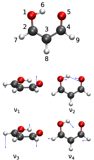
Malonaldehyde has been extensively studied in the past Ferro-Costas and Fernández-Ramos 2020 and presents a benchmark system for the development of quantum dynamical methods. Most recent calculations on the same PES using exact quantum methods were obtained using MCTDH by Hammer and Manthe Hammer and Manthe 2012 and Schröder and Meyer Schröder and Meyer 2014 and show a good level of agreement with experimental results Lüttschwager et al. 2013. We use the results of Ref. Hammer and Manthe 2012 for comparison, as they report TSs for a number of vibrationally excited states having a large transition dipole moment and are believed to be more accurate Schröder and Meyer 2014.
Local harmonic and VSCF/VCI energies, calculated in a -mode representation of the single-well potential, as described in Appendix C, for the lowest 8 vibrational states, that we consider below, are shown in Table 1. The ground state is labelled GS, while the excited states are labelled by the frequencies of the excited normal modes, numbered in the order of increasing frequency in the subscript, and separated by a ‘’ sign for multiple excitations. A noticable shift can be observed between all harmonic and VCI energies in Table 1 due to anharmonicity, but the order in energies remains unchanged. The lowest four normal modes that can get excited in the lowest 8 local vibrational states, and that play a role in our calculations below, are depicted in Figure 3. Higher vibrational states become more densely spaced in energy and start to mix vibrational modes at minima. Our approach relies on being able to uniquely define the excited normal modes at minima for each local vibrational state considered, because the instanton wavefunctions, that are used to calculate the TM elements that connect these states, tend to harmonic oscillator eigenstates at minima. Moreover, a higher density of states at higher energies would require inclusion of many additional states in the tunneling matrix, which are not known as precisely as for the low-lying states and would thus degrade the accuracy. We limit ourselves, therefore, to the lowest 8 local states in the studies of tunneling spectra of malonaldehyde below.
| State | Harmonic | VCI |
|---|---|---|
| GS | ||
The TM elements in the matrix that connect the two sets of local states in the L and R wells are calculated using the JFI method and listed in Table 2. Both minima of malonaldehyde belong to the symmetry group and its local vibrational states can be classified according to the irreducible representation of the excited normal mode at the minimum. The symmetry is preserved along the MAP, so that the TM elements that connect normal modes of different symmetry vanish exactly, as seen in Table 2.
In a matrix model, only the diagonal elements of matrix are used and the degenerate vibrational states of L/R wells are split into doublets. Equivalent results are obtained using the first-order perturbation theory for degenerate states, yielding the TS of . Energies of the GS and the first 3 excited states obtained in this manner already show a good agreement with the MCTDH results of Ref. Hammer and Manthe 2012, as can be seen in Table 3 (from the second and the last column). The vibrational states are numbered in order of increasing energy in Table 3. The wavefunction content, obtained from the eigenvectors of the TM, is listed in Table 4 and can be used to identify states in Table 3 in terms of the excited normal modes.
The TSs for the GS and the singly excited modes in the TM model are obtained as , , , , . The MCTDH results Hammer and Manthe 2012 for the TSs in the same states are , , , , . Differences in TSs, apart from the - and -excited modes are well within the estimated error of the MCTDH calculations, which validates the accuracy of our approach. The mode corresponds to the longitudinal mode as it lies parallel to the MAP at minima. The excitation of this mode effectively lowers the barrier of the tunneling motion and the instanton theory is known to overestimate TSs in the shallow tunneling regime Richardson and Althorpe 2011; Eraković and Cvitaš 2020. The wavefunction also penetrates deeper into the barrier where the anharmonic effects are larger and the VCI energies degrade as a result. Thus the accuracy in absolute energies in Table 3 is also expected to be affected for these states. The large increase in the TS for the excitation of the longitudinal mode is, however, expected Eraković and Cvitaš 2020 as confirmed by our results. The TS for the mode is overestimated by a factor of two. This is most likely due to the anharmonicity along this normal mode, indicated by the large difference between the harmonic (268.57 ) and VCI (330.19 ) energies. Since the TS for the pair of states is significantly suppressed compared to the GS, the frequency and energy in its direction change substantially along the MAP. Therefore, if the anharmonicity also changes significantly, it could cause the observed discrepancy. As an aside, we also note here that the other TSs computed using MCTDH in Ref. Hammer and Manthe 2012, which do not result in the mixture of normal modes at minima, are , , and , and are in good agreement with the values we obtain using JFI theory as , , and .
| No. | ||||
|---|---|---|---|---|
| 1 | 14670.15 | 14668.69 | 14667.08 | 14671.3 |
| 2 | 14694.76 | 14693.54 | 14692.76 | 14694.8 |
| 3 | 14998.31 | 14999.77 | 14987.74 | 14941.5 |
| 4 | 15005.95 | 15005.60 | 15005.09 | 15008.2 |
| 5 | 15019.35 | 15018.91 | 15018.54 | 15014.9 |
| 6 | 15086.70 | 15087.92 | 15077.14 | 15005.4 |
| 7 | 15125.42 | 15125.86 | 15125.14 | 15108.3 |
| 8 | 15142.47 | 15142.82 | 15142.04 | 15124.6 |
| 9 | 15243.00 | - | 15249.04 | - |
| 10 | 15257.21 | - | 15263.41 | - |
| 11 | 15266.89 | - | 15266.12 | - |
| 12 | 15274.07 | - | 15273.84 | 15249.6 |
| 13 | 15289.71 | - | 15291.11 | 15268.4 |
| 14 | 15314.85 | - | 15316.14 | - |
| 15 | 15357.47 | - | 15358.55 | - |
| 16 | 15394.71 | - | 15407.27 | - |
We next consider construcing the tunneling matrix using 4 local states in each well. This takes into account interactions between the doublets considered above, whereby only the states of the same symmetry interact. If the states of the same symmetry are well separated with respect to the size of their TM element, the shift in energy can also be computed using the second-order perturbation theory. When 4 local states are taken into account in the TM model, slight shifts are observed in the GS and -doublets in Figure 9 (left-side spectrum). The absolute energies change by , while perturbation theory gives the shift of . However, the change in the TS is negligible.
In the TM model, consisting of 8 local states in each well, a strong interaction with the doubly-excited mode causes a significant shift in the energies of the GS and the -excited doublets as well as their splittings. The TSs change from to and from to , which can clearly be observed in Figure 9 (right-side spectrum). A particularly strong mixing also occurs between the doubly-excited mode and the doubly-excited mode, for which the lower levels in the doublets are very close in energy ( ) and they interact strongly ( in Table 2). The mixing results in visible changes in the dominant coefficients of TM eigenvectors in Table 4 and leads to observable energy shifts. Furthermore, singly-excited mode interacts and mixes with the doubly-excited mode, which results in the change of its TS from to , which is in closer agreement with the MCTDH value of . Finally, we remark that the TS of the doubly-excited state amounts to which is in good agreement with obtained by Schröder and Meyer Schröder and Meyer 2014.
The above results clearly show that the interactions of different vibrational states can have a non-negligible effect, both, on the absolute values of the vibrational energies and on the values of the tunneling splittings. This effect is especially pronounced if two or more states of the same symmetry are close in energy and if the TM elements that connect them are large. This scenario is expected to play a significant role in the higher vibrationally excited states, where the density of states becomes larger and the interactions increase due to the presence of multiple excitations.
| No. | Pairs | (8) |
|---|---|---|
| 1 | ||
| 2 | ||
| 3 | ||
| 4 | ||
| 5 | ||
| 6 | ||
| 7 | ||
| 8 | ||
| 9 | ||
| 10 | ||
| 11 | ||
| 12 | ||
| 13 | ||
| 14 | ||
| 15 | ||
| 16 | ||
III.3 PARTIALLY DEUTERATED MALONALDEHYDE
In the previous Subsection, we have learned what accuracy one might expect in the calculation of the tunneling spectra of malonaldehyde through comparison with the exact QM results. We now consider the partially deuterated (PD) malonaldehyde, where hydrogen in the position 7/9 is substituted by deuterium (see Figure 3) and the system in no longer symmetric. Since deuterium is not placed in equivalent positions in the two minima, their local vibrational frequencies and energies are no longer equal, even though the PES remains unchanged. The particular choice of deuteration was chosen for our study because the mixing angle in its GS was determined experimentally by Baughcum et al Baughcum et al. 1981 and the TS by Jahr et al Jahr, Laude, and Richardson 2020 using RPI method. Furthermore, the size of the relative energy shifts between the left and right minimum is comparable to the size of the TM elements, which makes the system interesting in that both the VCI energies and the instanton TM elements are expected to make a significant contribution to the TSs in this system.
| State | Harmonic | VCI | ||
|---|---|---|---|---|
| D7 | D9 | D7 | D9 | |
| GS | ||||
| No. | |||
|---|---|---|---|
| 1 | 13974.27 | 13972.91 | 13971.48 |
| 2 | 14016.96 | 14015.52 | 14014.49 |
| 3 | 14296.86 | 14298.42 | 14286.79 |
| 4 | 14295.75 | 14295.44 | 14294.91 |
| 5 | 14314.69 | 14313.95 | 14313.54 |
| 6 | 14391.55 | 14392.78 | 14381.17 |
| 7 | 14383.28 | 14384.05 | 14383.32 |
| 8 | 14446.16 | 14446.45 | 14445.64 |
| 9 | 14540.00 | - | 14537.31 |
| 10 | 14549.82 | - | 14549.32 |
| 11 | 14541.38 | - | 14556.57 |
| 12 | 14560.53 | - | 14561.08 |
| 13 | 14597.33 | - | 14598.21 |
| 14 | 14596.99 | - | 14598.33 |
| 15 | 14641.54 | - | 14642.66 |
| 16 | 14696.90 | - | 14709.18 |
In the PD malonaldehyde, the isotopic substitution causes a significant lowering of the zero-point energy, given in Table 5, from to for D7 minimum and to for D9 minimum. Additionally, the excitation energies for the first 7 excited states decrease as well, by up to . As a result, the vibrational states are more closely spaced, see Figure 10, and larger interstate L/R mixings are expected.
The normal modes in PD malonaldehyde are qualitatively similar to the homoisotopic malonaldehyde, depicted in Figure 3. The ordering of local single-well states, labelled by the excited normal mode at minimum, is also preserved upon deuteration, with the exception of the and states, which exchange order. The TM elements, shown in Table 6, are remarkably similar to the homoisotopic malonaldehyde, which indicates that the wavefunctions in the barrier region are not significantly affected by the asymmetry. The error estimates due to the variation of the position of the dividing plane are shown in parentheses in Table 6, and are discussed in more detail in Appendix B.
We again consider pairwise interactions of the corresponding states in a TM model. This is possible since the normal modes at both minima can approximately be mapped to one another using a symmetry operation. The pairs of states are no longer degenerate in this case, and the first-order perturbation theory cannot be used to estimate the TSs. Instead, the TS, obtained from the eigenvalues of the TM, is seen to be equal to the local energy difference corrected by the second-order perturbative terms,
| (12) |
where, in the last line of Eq. (12), we assumed that the TM element . This assumption is certainly violated if there are other local states which are energetically close and coupled by the TM elements that are comparable in size.
The TM element for the GS is using JFI method, which is in excellent agreement with obtained by Jahr et al Jahr, Laude, and Richardson 2020 using RPI. The mixing angle for the GS was estimated experimentally by Baughcum et al Baughcum et al. 1981 at . Ref. Jahr, Laude, and Richardson 2020 estimates the angle at , using local harmonic energies. Using VCI energies, we estimate the mixing angle to be , which indicates that the anharmonicity is indeed responsible for a decrease in its value, as speculated by Jahr et al Jahr, Laude, and Richardson 2020. We were also able to estimate the effect of the inclusion of other local vibrational states on the mixing angle from the components of the TM eigenvectors in Table 8 as
| (13) |
which gives . It thus appears that the inclusion of additional interactions corrects the mixing angle towards the experimental value.
Changes in the vibrational levels of the excited states in the and the matrix models, listed in Table 7, are qualitatively similar to the homoisotopic malonaldehyde due to the similarity in their TM elements. The vibrational tunneling spectrum is shown graphically in Figure 10. One significant difference here is that some doublet states change order of their components after the inclusion of additional vibrational states in the model due to their proximity in energy after deuteration, as seen in Figure 10. Another difference is the absence of symmetry in the wavefunctions with respect to the symmetry operation that connects the minima in the homoisotopic case. As a result, the extensions of the model to higher dimensionality matrix models will mix both, the lower and the higher components of doublets, with all other doublet states. Finally, due to the proximity of vibrational states, the lower components of the , and doublets are significantly mixed, as can be seen in Table 8. This mixing between the states changes their energies, but it is also expected to affect the intensity of the transition to the state, as its component (see Table 8) has a higher transition dipole moment, being the singly excited state.
| No. | Pairs | (8) |
|---|---|---|
| 1 | ||
| 2 | ||
| 3 | ||
| 4 | ||
| 5 | ||
| 6 | ||
| 7 | ||
| 8 | ||
| 9 | ||
| 10 | ||
| 11 | ||
| 12 | ||
| 13 | ||
| 14 | ||
| 15 | ||
| 16 | ||
IV Conclusions
We applied a combination of VCI and instanton theory to calculate vibrational tunneling spectra of some exemplary double-well systems in full dimensionality at a much reduced computational cost in comparison with the exact QM methods. The VCI method was used to compute the single-well vibrational spectra, while the recently developed instanton method was used to determine the wavefunctions inside the barrier that separates the wells at a comparatively negligible computational cost. The interaction between the states of different wells was obtained from the Herring formula evaluated at a dividing surface inside the barrier. Herring formula was rederived in an extended matrix model () and the size of the associated leading error term was analysed.
The accuracy of our approach was first tested on a model 2D system. It was shown that the JFI method can be used to compute TM elements that connect states in inequivalent wells and that have excitations in different normal modes. The energy levels of an asymmetric system exhibit avoided crossings with the variation of frequency or depth of one well relative to the other. The VCI calculation of local energies proved to be necessary in order to reproduce the exact QM results with high accuracy. The method was then tested on malonadehyde in full dimensionality, where good agreement was achieved with the exact MCTDH results in the absolute energies and the splittings. It was shown that the extension of the standard model to include more states can influence the vibrational energies. The results are not affected dramatically in the case of malonaldehyde, but it was shown that the model is able to accommodate the additional vibrational states in the systems where they lie close in energy.
Finally, the method was used to calculate the vibrational spectrum of the low-lying states in partially deuterated malonaldehyde, which is near the computational limit of the presently available exact QM methods. The ground state mixing angle was compared to the experiment and the influence of including additional vibrational states was shown to affect the angle and the order of some states in the spectrum.
The method is expected to perform well for mid-sized molecules, where rotational motion, which is neglected in this work, can be separated from the tunneling dynamics, and for moderately anharmonic systems with high barriers and, consequently, small tunneling splittings. It is exactly in these circumstances that the exact QM methods come at a prohibitive computational cost. The developed combined approach can be used to calculate the low-lying vibrational spectra in systems with arbitrary number of wells, which are not necessarily related by symmetry. This makes the method particularly suitable to the studies of clusters, e.g., for the assignment of spectra in water clusters, which feature multiple minima and high barriers in their bifurcation dynamics (where hydrogen bonds are broken and reformed). The computational cost of our approach is concentrated in solving the single-well spectra separately. The instanton theory can also be combined with other high-level methods, instead of VCI, and the combined, dual-level, approach can be used to calculate tunneling spectra in general multidimensional asymmetric well systems, beyond molecular applications and chemistry.
Acknowledgements.
This work was fully supported by Croatian Science Foundation Grant No. IP-2020-02-9932.Appendix A MAP invariance with respect to the addition of a switching function
We show below that the addition of a function , which only depends on the coordinate along the path, to the potential,
| (14) |
does not change the shape of the MAP, but only scales the imaginary time parameter . The statement is valid if the function does not change the position or shape of the minima, i.e., it satisfies
| (15) |
and is negligible in comparison with the potential in the region between the minima, .
Path is the characteristic for potential and it satisfies
| (16) |
where is the arc length distance along the path. We define the scaled imaginary time as
| (17) |
The scaled momentum then becomes
| (18) |
The momentum vector transforms as
| (19) |
whereas the acceleration becomes
| (20) |
where the symbol in the subscript denotes the component of the vector that is perpendicular to the path. Now, if the function satisfies the conditions in Eq. (15) and is significantly smaller than the potential, the second term on the right hand side of Eq. (20) is small everywhere on the path in comparison to the gradient of the potential and can be ignored. Eq. (20) then takes the form of the equation of characteristic, but on the modified potential .
Appendix B Dependence of tunneling matrix elements on the position of the dividing plane
TM elements between the states with, at most, one excitation (, ) can be expressed as
| (21) |
where the contribution of terms in Eq. (9) has been neglected. It is known that, unless these terms exclusively contribute to the TM elements, they introduce the dependence of the TM element on the connection point Eraković and Cvitaš 2020. Therefore, we omit them from the treatment here to separate the effect of terms from the effect of asymmetry in the dependence of the TM element with the variation of the connection point . The case of multiple excitations, as well as that of the terms, can be derived in an analogous fashion.
Dependence on the position of the connection point can be determined by differentiating the TM element in Eq. (21) with respect to . Small changes in the connection point correspond to the addition of function of the following form
| (22) |
to the potential in the action integral, where denotes the change in the connection point. As discussed in Appendix A, the addition of does not change the shape of the path. The differentiation can thus be performed on the same path. Furthermore, if the connection point is located deep inside the barrier, we can approximate
| (23) |
Following the differentiation, as described in Ref. Eraković and Cvitaš 2020, we obtain
| (24) |
where are the energies of the local L/R wavefunctions and is the matrix projected onto the space orthogonal to the MAP. From Eq. (24), it is evident that the TM element will only be invariant with respect to variation in if the two local L/R states are in resonance. Otherwise, the TM element depends on the position of the connection point and the dependence is stronger for a larger mismatch in the local energies.
The dependence on the connection point can be traced to the neglected integral in the derivation of Herring formula in Eq. (3) involving term. Inclusion of this term, transforms the formula for the TM element into
| (25) |
where the second integral is taken over the space on the ‘left’ side of the dividing plane. We then differentiate the extended expression, Eq. (25), with respect to , and observe that the derivative of the additional term in Eq. (25) is the integral over the dividing plane. The derivative of the TM element becomes
| (26) |
where use has been made of Eq. (24). We note now that the surface integral in Eq. (26) differs from the ‘old version’ of only by the momentum term . However, this factor is taken to be constant on the dividing plane and it can be taken out of the integral, which leads to
| (27) |
While it would seem obvious to use the instanton wavefunctions in Eq. (6) and compute the additional term that arises in Eq. (26) in order to eliminate the dependence on , the semiclassical approximation breaks down beyond the barrier region and would lead to a divergence of the integral. We are thus left with no option but to neglect the term and treat it as a source of error in the TM element.
We tried to estimate the size of the error term, introduced above, by calculating the overlap of the harmonic oscillator wavefunctions centered at the two minima. The overlap is obtained following the method of Ref. Berger, Fischer, and Klessinger 1998, where it was used to calculate Frank-Condon factors between the shifted harmonic oscillators. The calculation requires the knowledge of molecular geometries and harmonic frequencies in the two minima and does not add to the overall computational cost. The errors for the partially deuterated malonaldehyde were found to be small and are listed in the parenthesis in Table 6. We found that it was safe to neglect the error terms unless the connection point is moved far from the position of the barrier top, or unless the energy difference between the two states is large in relation to the barrier height. However, we note that as the energy difference increases, the contribution of the TM element to the energy level decreases, as seen from the second-order perturbation treatment,
| (28) |
Since are expected to be small in the deep tunneling regime, the contributions of the states that lie far from the resonance quickly approach zero. Thus, even for larger energy differences, the computed energy levels remain stable.
Dependence of the TM elements on the position of the dividing plane was also tested by moving the dividing plane from to , where is the MAP length. All the matrix elements displayed monotonous dependence on , with an inflection point located near the position of the barrier top, and a region of relative stability around it. As the dividing plane is moved away from the barrier top, some TM elements begin to change significantly. These TM elements connect the states with a significant disparity in their local energies. For example, the TM elements between the state and the GS or the -excited state change from to and from to , respectively. However, a large energy difference between the involved states also implies that the TM elements do not profoundly affect the overall energy. The GS TS varies by in this region. If we limit ourselves to the region between and , the variation of the GS TS is only , which is within the error of the VCI method used to compute the local energies. Similar errors are observed for the other energy levels. The method thus gives best results when the dividing plane is placed in the vicinity of the barrier top.
Appendix C Vibrational self consistent field (VSCF) and vibrational configuration interaction (VCI)
The idea behind the VSCF approach is to approximate the vibrational wavefunction by a Hartree product of single-mode (1M) functions as
| (29) |
where is the -th normal mode coordinate. The above form can efficiently be employed in combination with the -mode representation Bowman, Carter, and Huang 2003; Rauhut 2004 of the potential
| (30) |
In this paper, the expansion was truncated at the two-mode (2M) terms. Using wavefunction in Eq. (29) and variational principle, it can be shown Carter, Bowman, and Handy 1998; Christoffel and Bowman 1982; Bowman, Christoffel, and Tobin 1979 that the optimal 1M functions satisfy a set of coupled 1M equations
| (31) |
which can be solved via an SCF algorithm. The 1M functions are expanded in a basis set . In this paper, the lowest states of the harmonic oscillator (HO) are used. The 1M and 2M potential energy terms in Eq. (30) are fitted to polynomials of order as
| (32) |
These choices enable us to compute the potential matrix elements exactly. For that purpose, we calculate the matrices , that represent operators in the HO basis. This can be done recursively using ladder operators
| (33) |
The matrices are then stored and the SCF algorithm is started using the initial guess . The effective Hamiltonian in Eq. (31) is constructed for each mode in the HO basis, diagonalized and the obtained 1M functions corresponding to the lowest eigenvalue taken as new . Once VSCF has converged, the obtained virtual 1M functions are used to construct the VCI Hamiltonian
| (34) |
The matrix elements of are computed using matrices and the coefficients of 1M functions in the HO basis. Its eigenvalues represent VCI energies, while the eigenvectors can be used to determine the dominant configuration and tell us which normal modes are excited in the particular state.


References
- Bell (1980) R. P. Bell, The Tunnel Effect in Chemistry (Chapman and Hall, London, 1980).
- Hund (1927) F. Hund, Z. Phys. 43, 805 (1927).
- Benderskii, Makarov, and Wight (1994) V. A. Benderskii, D. E. Makarov, and C. A. Wight, Chemical Dynamics at Low Temperatures, Adv. Chem. Phys., Vol. 88 (Wiley, New York, 1994).
- Urban et al. (1981) Š. Urban, V. Špirko, D. Papoušek, J. Kauppinen, S. Belov, L. Gershtein, and A. Krupnov, J. Mol. Spectrosc. 88, 274 (1981).
- Firth et al. (1991) D. W. Firth, K. Beyer, M. A. Dvorak, S. W. Reeve, A. Grushow, and K. R. Leopold, J. Chem. Phys. 94, 1812 (1991).
- Mengesha et al. (2013) E. T. Mengesha, J. Sepioł, P. Borowicz, and J. Waluk, J. Chem. Phys. 138, 174201 (2013).
- Tanaka et al. (2004) K. Tanaka, M. Toshimitsu, K. Harada, and T. Tanaka, J. Chem. Phys. 120, 3604 (2004).
- Cvitaš and Richardson (2020) M. T. Cvitaš and J. O. Richardson, in Molecular Spectroscopy and Quantum Dynamics, edited by R. Marquardt and M. Quack (Elsevier, 2020) Chap. 9, pp. 301–326.
- Jahr, Laude, and Richardson (2020) E. Jahr, G. Laude, and J. O. Richardson, J. Chem. Phys. 153, 094101 (2020).
- Baughcum et al. (1981) S. L. Baughcum, R. W. Duerst, W. F. Rowe, Z. Smith, and E. B. Wilson, J. Am. Chem. Soc. 103, 6296 (1981).
- Zhang et al. (1995) D. H. Zhang, Q. Wu, J. Z. H. Zhang, M. von Dirke, and Z. Bačić, J. Chem. Phys. 102, 2315 (1995).
- Šmydke et al. (2019) J. Šmydke, C. Fábri, J. Sarka, and A. G. Császár, Phys. Chem. Chem. Phys. 21, 3453 (2019).
- Liu et al. (1996) K. Liu, M. G. Brown, M. R. Viant, J. D. Cruzan, and R. J. Saykally, Mol. Phys. 89, 1373 (1996).
- Eraković and Cvitaš (2021) M. Eraković and M. T. Cvitaš, Phys. Chem. Chem. Phys. 23, 4240 (2021).
- González, Mó, and Yáñez (1997) L. González, O. Mó, and M. Yáñez, J. Phys. Chem. A 101, 9710 (1997).
- Bondybey, Haddon, and Rentzepis (1984) V. E. Bondybey, R. C. Haddon, and P. M. Rentzepis, J. Am. Chem. Soc. 106, 5969 (1984).
- Oppenländer et al. (1989) A. Oppenländer, C. Rambaud, H. P. Trommsdorff, and J.-C. Vial, Phys. Rev. Lett. 63, 1432 (1989).
- Hall et al. (2007) B. V. Hall, S. Whitlock, R. Anderson, P. Hannaford, and A. I. Sidorov, Phys. Rev. Lett. 98, 030402 (2007).
- Takahashi et al. (2011) S. Takahashi, I. S. Tupitsyn, J. van Tol, C. C. Beedle, D. N. Hendrickson, and P. C. E. Stamp, Nature 476, 76 (2011).
- Johnson et al. (2005) P. R. Johnson, W. T. Parsons, F. W. Strauch, J. R. Anderson, A. J. Dragt, C. J. Lobb, and F. C. Wellstood, Phys. Rev. Lett. 94, 187004 (2005).
- Felker and Bačić (2019) P. M. Felker and Z. Bačić, J. Chem. Phys. 151, 024305 (2019).
- Schröder and Meyer (2014) M. Schröder and H.-D. Meyer, J. Chem. Phys. 141, 034116 (2014).
- Hammer and Manthe (2012) T. Hammer and U. Manthe, J. Chem. Phys. 136, 054105 (2012).
- Leforestier, Szalewicz, and van der Avoird (2012) C. Leforestier, K. Szalewicz, and A. van der Avoird, J. Chem. Phys. 137, 014305 (2012).
- Vaillant, Wales, and Althorpe (2018) C. L. Vaillant, D. J. Wales, and S. C. Althorpe, J. Chem. Phys. 148, 234102 (2018).
- Vaillant, Wales, and Althorpe (2019) C. L. Vaillant, D. J. Wales, and S. C. Althorpe, J. Phys. Chem. Lett. 10, 7300 (2019).
- Benderskii et al. (1997) V. Benderskii, E. Vetoshkin, S. Grebenshchikov, L. von Laue, and H. Trommsdorff, Chem. Phys. 219, 119 (1997).
- Smedarchina, Siebrand, and Fernández-Ramos (2012) Z. Smedarchina, W. Siebrand, and A. Fernández-Ramos, J. Chem. Phys. 137, 224105 (2012).
- Richardson and Althorpe (2011) J. O. Richardson and S. C. Althorpe, J. Chem. Phys. 134, 054109 (2011).
- Mil’nikov and Nakamura (2001) G. V. Mil’nikov and H. Nakamura, J. Chem. Phys. 115, 6881 (2001).
- Eraković, Vaillant, and Cvitaš (2020) M. Eraković, C. L. Vaillant, and M. T. Cvitaš, J. Chem. Phys. 152, 084111 (2020).
- Cvitaš and Althorpe (2016) M. T. Cvitaš and S. C. Althorpe, J. Chem. Theory Comput. 12, 787 (2016).
- Cvitaš (2018) M. T. Cvitaš, J. Chem. Theory Comput. 14, 1487 (2018).
- Mil’nikov, Ishida, and Nakamura (2006) G. V. Mil’nikov, T. Ishida, and H. Nakamura, J. Phys. Chem. A 110, 5430 (2006).
- Mil’nikov, Kühn, and Nakamura (2005) G. Mil’nikov, O. Kühn, and H. Nakamura, J. Chem. Phys. 123, 074308 (2005).
- Vaillant and Cvitaš (2018) C. Vaillant and M. T. Cvitaš, Phys. Chem. Chem. Phys. 20, 26809 (2018).
- Zwart et al. (1991) E. Zwart, J. J. ter Meulen, W. L. Meerts, and L. H. Coudert, J. Mol. Spectrosc. 147, 27 (1991).
- Keutsch, Cruzan, and Saykally (2003) F. N. Keutsch, J. D. Cruzan, and R. J. Saykally, Chem. Rev. 103, 2533 (2003).
- Richardson et al. (2016) J. O. Richardson, C. Pérez, S. Lobsiger, A. A. Reid, B. Temelso, G. C. Shields, Z. Kisiel, D. J. Wales, B. H. Pate, and S. C. Althorpe, Science 351, 1310 (2016).
- Richardson et al. (2013) J. O. Richardson, D. J. Wales, S. C. Althorpe, R. P. McLaughlin, M. R. Viant, O. Shih, and R. J. Saykally, J. Phys. Chem. A 117, 6960 (2013).
- Cvitaš and Richardson (2019) M. T. Cvitaš and J. O. Richardson, Phys. Chem. Chem. Phys. 22, 1035 (2019).
- Eraković and Cvitaš (2020) M. Eraković and M. Cvitaš, J. Chem. Phys. 153, 134106 (2020).
- Mil’nikov and Nakamura (2005) G. V. Mil’nikov and H. Nakamura, J. Chem. Phys. 122, 124311 (2005).
- Garg (2000) A. Garg, Am. J. Phys. 68, 430 (2000).
- Herring (1962) C. Herring, Rev. Mod. Phys. 34, 631 (1962).
- Cesi, Rossi, and Testa (1991) F. Cesi, G. C. Rossi, and M. Testa, Ann. Phys. 206, 318 (1991).
- Mugnai and Ranfagni (1985) D. Mugnai and A. Ranfagni, Phys. Lett. A 109, 219 (1985).
- Leggett et al. (1987) A. J. Leggett, S. Chakravarty, A. T. Dorsey, M. P. A. Fisher, A. Garg, and W. Zwerger, Rev. Mod. Phys. 59, 1 (1987).
- Dekker (1987) H. Dekker, Physica A 146, 375 (1987).
- Song (2008) D.-Y. Song, Ann. Phys. 323, 2991 (2008).
- Song (2015) D.-Y. Song, Ann. Phys. 362, 609 (2015).
- Halataei and Leggett (2017) S. M. H. Halataei and A. J. Leggett, arXiv preprint arXiv:1703.05758 (2017).
- Siebrand, Smedarchina, and Fernández-Ramos (2013) W. Siebrand, Z. Smedarchina, and A. Fernández-Ramos, J. Chem. Phys. 139, 021101 (2013).
- Benderskii, Vetoshkin, and Trommsdorff (1999) V. Benderskii, E. Vetoshkin, and H. Trommsdorff, Chem. Phys. 244, 299 (1999).
- Benderskii et al. (2000) V. Benderskii, E. Vetoshkin, I. Irgibaeva, and H. Trommsdorff, Chem. Phys. 262, 393 (2000).
- Carter, Bowman, and Handy (1998) S. Carter, J. M. Bowman, and N. C. Handy, Theor. Chim. Acta 100, 191 (1998).
- Christoffel and Bowman (1982) K. M. Christoffel and J. M. Bowman, Chem. Phys. Lett. 85, 220 (1982).
- Bowman, Christoffel, and Tobin (1979) J. M. Bowman, K. Christoffel, and F. Tobin, J. Phys. Chem. 83, 905 (1979).
- Bowman, Carter, and Huang (2003) J. M. Bowman, S. Carter, and X. Huang, Int. Rev. Phys. Chem. 22, 533 (2003).
- Rauhut (2004) G. Rauhut, J. Chem. Phys. 121, 9313 (2004).
- Wang et al. (2008) Y. Wang, B. J. Braams, J. M. Bowman, S. Carter, and D. P. Tew, J. Chem. Phys. 128, 224314 (2008).
- Ferro-Costas and Fernández-Ramos (2020) D. Ferro-Costas and A. Fernández-Ramos, in Tunnelling in Molecules: Nuclear Quantum Effects from Bio to Physical Chemistry, edited by J. Kästner and S. Kozuch (Royal Society of Chemistry, 2020) Chap. 9, pp. 283–327.
- Lüttschwager et al. (2013) N. O. Lüttschwager, T. N. Wassermann, S. Coussan, and M. A. Suhm, Mol. Phys. 111, 2211 (2013).
- Berger, Fischer, and Klessinger (1998) R. Berger, C. Fischer, and M. Klessinger, J. Phys. Chem. A 102, 7157 (1998).