OU-HEP-211030
The cosmological moduli problem and naturalness
Kyu Jung Bae111
1
Email: kyujung.bae@knu.ac.kr,
Howard Baer2,311
1
Email: baer@nhn.ou.edu ,
Vernon Barger322
2
Email: barger@pheno.wisc.edu ,
and Robert Wiley Deal2,333
3
Email: rwileydeal@ou.edu
1Dep’t of Physics,
Kyungpook National University, Daegu 41566, Korea
2Homer L. Dodge Dep’t of Physics and Astronomy,
University of Oklahoma, Norman, OK 73019, USA
3Dep’t of Physics,
University of Wisconsin, Madison, WI 53706, USA
Nowadays, the cosmological moduli problem (CMP) comes in three parts: 1. potential violation of Big-Bang nucleosynthesis (BBN) constraints from late decaying moduli fields, 2. the moduli-induced gravitino problem wherein gravitinos are overproduced and their decays violate BBN or dark matter overproduction bounds and 3. the moduli-induced lightest SUSY particle (LSP) overproduction problem. Also, the CMP may be regarded as either a problem or else a solution to scenarios with dark matter over- or under-production. We examine the cosmological moduli problem and its connection to electroweak naturalness. We calculate the various two-body decay widths of a light modulus field into MSSM particles and gravitinos within general supersymmetric models. We include both phase space and mixing effects. We examine cases without and with helicity suppression of modulus decays to gravitinos (cases 1 & 2) and/or gauginos (cases A & B). For case B1, we evaluate regions of gravitino mass vs. modulus mass parameter space constrained by BBN, by overproduction of gravitinos and by overproduction of neutralino dark matter, along with connections to naturalness. For this case, essentially all of parameter space is excluded unless TeV with . For a potentially most propitious case B2 with decay to Higgs and matter turned off, then modulus branching fractions to SUSY and to gravitinos become highly suppressed at large . But since the modulus number density increases faster than the branching fractions decrease, there is still gross overproduction of neutralino dark matter. We also show that in this scenario the thermally produced gravitino problem is fixed by huge entropy dilution, but non-thermal gravitino production from moduli decay remains a huge problem unless it is kinematically suppressed with . In a pedagogical appendix, we present detailed calculations of modulus field two-body decay widths.
1 Introduction
Supersymmetric (SUSY) models of particle physics have long been the dominant paradigm for Beyond the Standard Model physics [1, 2] due to their clean solution to the gauge hierarchy problem and their capacity to explain the dark matter in the universe. They are also supported by a variety of virtual effects, including 1. gauge coupling unification [3], 2. top-Yukawa induced radiative breaking of electroweak symmetry [4], 3. agreement between theory and experiment on the mass of the newly discovered Higgs boson [5] and 4. precision electroweak measurements [6] which actually favor a (heavy) TeV-scale SUSY spectrum over the Standard Model (SM). In contrast to these success stories, SUSY models have been under seige lately due to 1. lack of superpartners at LHC with mass below early naturalness estimates (the SUSY naturalness or little hierarchy problem) and 2. lack of a clear WIMP signal at direct or indirect dark matter detection experiments. The first of these problems has been dispatched by realizing that conventional naturalness measures overestimate finetuning in supersymmetric11 1 The log derivative measure was typically applied assuming multiple independent soft SUSY breaking parameters in the low energy effective field theory (EFT) which leads to overestimates of finetuning [7, 8, 9] compared to more complete theories wherein the soft parameters are correlated. The high scale measure abandons some dependent contributions which lead to cancellations when fully included [7, 8, 9]. models. Applying the more conservative, parameter-independent measure [10, 11] allows for gluinos and squarks well beyond current LHC mass limits while only the several neutral and charged higgsinos need lie close to the electroweak scale: . Thus, in natural SUSY, we expect the usual dark matter candidate, the lightest neutralino, to be dominantly higgsino-like.
The second problem, the lack of a clear WIMP signal, was perhaps already presaged by the difficulty of thermally-produced SUSY WIMPs to make up the measured dark matter relic density [12]. Binos tend to thermally overproduce dark matter due to their low annihilation cross sections in the early universe unless special mechanisms such as co-annihilation [13, 14] or resonance annihilation [15, 16] or tuning/tempering [17, 18] are invoked. Wino dark matter, as expected in anomaly-mediation models, thermally underproduce the measured abundance for TeV while higgsino-like WIMPs underproduce DM for TeV (well beyond expected bounds from naturalness which require GeV). One way around the underproduction issue is to invoke the axion solution to the strong CP problem so that both axions and WIMPs make up the dark matter [19, 20]. The relic density calculation then requires solving eight coupled Boltzmann equations which include contributions from axions, axinos, saxions, neutralinos, and gravitinos [21, 22].
An alternative solution to the WIMP underproduction problem has been to invoke non-thermal DM production via one or more hypothesized moduli fields– gravitationally coupled scalar fields with a classically flat potential. Moduli fields are highly motivated from compactified string theory where they determine the size and shape of the 6-7 compact dimensions of the required 10-11 dimensional spacetime. The properties of the moduli fields are critical for predictivity in string theory since their vacuum expectation values (vevs) determine the otherwise free parameters of the low energy EFT such as gauge and Yukawa couplings and soft SUSY breaking terms. A primary concern of string phenomenologists is to understand moduli stabilization: how perturbative or non-perturbative effects can stabilize the moduli so that their vevs can be determined. Two popular schemes for moduli stabilization in II-B string theory include the KKLT [23] approach, where complex structure moduli are stabilized by flux to gain ultra-high (decoupled) masses whilst the Kähler moduli are assumed stabilized by non-perturbative effects and may gain much lower masses. KKLT is characterized by a mass hierarchy where is the presumed mass of the lightest Kähler modulus [24]. The second scheme, the large volume scenario (LVS) [25, 26], stabilizes Kähler moduli via a combination of perturbative and non-perturbative contributions to the scalar potential which arise from compactification on a “swiss cheese” type of CY manifold where one modulus sets the overall size of the cheese (large volume) and a second modulus describes the size of four-cycles (holes in the cheese). The volume modulus is expected as the lightest of the Kähler moduli and could have mass well below the soft SUSY breaking scale leading to the CMP.
Light moduli fields with TeV-scale masses ought to have a big impact on WIMP production rates in the early universe. They are expected to obtain Planckian field strengths during the inflationary epoch, but then start oscillating at temperatures when :
| (1) |
where is the reduced Planck mass. Since the oscillating moduli fields have the equation of state of matter, they will after some time come to dominate over the radiation produced from inflationary reheating. Due to the extremely large masses the light moduli may possess, these oscillations may actually begin during the reheating phase. In this case, expansion quickly dilutes their energy density relative to the radiation energy density, which at this phase is still being sourced by inflaton decay. The moduli will then decay at a temperature
| (2) |
into radiation (SM particles), dark matter and possibly dark radiation (neutrinos and axions). For a large enough modulus branching fraction into SUSY particles, then a vast overabundance of LSPs are produced from the modulus field decay so that they re-annihilate during the modulus decay period. Then the DM abundance is typically elevated beyond the thermally-produced value, but not as high as two-WIMPs-per modulus quanta. The yield variable for re-annihilating LSPs can be simply estimated [27, 28] and is found to be
| (3) |
leading to a non-thermally produced (NTP) relic abundance
| (4) |
For , the neutralino abundance will take its thermally-produced (TP) value while for the neutralino abundance is enhanced over the TP expectation by a factor . Of course, should also be higher than the temperature where Big Bang Nucleosynthesis (BBN) begins in order to not upset the successful prediction of light element abundances via the standard BBN calculation. This latter constraint typically requires rather heavy moduli field masses TeV since the gravitationally-coupled moduli decay late and ) (where is a model-dependent constant of order which is evaluated in this paper). Thus, by adjusting to high enough values, one can gain modulus field decay before the onset of BBN. This is the traditional solution to the BBN portion of the CMP.
From the above discussion, it should be apparent that the presence of late-decaying moduli fields in the early universe can be seen as both a problem and a solution for dark matter cosmology. It is problematic in that late decaying moduli can conflict with BBN (the original cosmological moduli problem) and/or overproduce dark matter (the moduli-induced dark matter problem). Also, if moduli can decay to gravitinos, then the gravitino overproduction can violate BBN or overproduce dark matter (this is the moduli-induced gravitino problem). In the case of thermally underproduced dark matter, then the presence of moduli can be invoked as a solution in that non-thermal dark matter production can bring the underproduced relic density into accord with measurements [29].
1.1 Brief review of previous work and plan for this work
We break this subsection up into papers concerned mainly with cosmological moduli as a problem and then those which regard it as a solution to other problems, mainly dark matter over- and under-production. Then we preview our perspective.
1.1.1 Cosmological moduli as a problem
The first paper to raise an alarm as to the cosmological moduli problem (CMP) was Coughlin et al. [30] who considered already in 1983 a single hidden sector gravitationally coupled scalar field in the supergravity-breaking Polonyi superpotential and how its decay would produce excess entropy which could disrupt baryogenesis. Dine et al. proposed multi-field hidden sectors that could allow the potentially disruptive scalar fields to settle to much lower field values [31]. Banks, Kaplan, and Nelson [32] noted in 1993 that hidden sector models required TeV to solve the CMP. This may conflict with naturalness and so make hidden sector (HS) models less palatable than the alternative of dynamical SUSY breaking (DSB). Also in 1993, de Carlos et al. [33] placed the CMP on a firm string foundation, emphasizing the generic problem in string theory of light dilaton and moduli fields with in place of the SUGRA-based Polonyi fields. They emphasize TeV to avoid the CMP. The tension between the required high modulus mass and the natural scale of SUSY breaking is noted. In Ref. [34], Randall and Thomas proposed a second stage of weak scale inflation due to the same moduli flat directions as begat the CMP, with only a few -foldings as a means to dilute the modulus field strength (see also Ref. [35]). Dine, Randall and Thomas[36] (DRT) pointed out the presence of Hubble-induced SUSY breaking masses for scalar fields during inflation and proposed some symmetry relating the minima of inflationary and post-inflationary potentials to set the modulus field strength to tiny values in the early universe. Dvali [37] proposed also that large contributions to moduli masses help set the modulus condensate to small values as a possible solution to the CMP. Lyth and Stewart proposed in 1995 [38] that the presence of flatons – scalar fields with weak scale masses but GeV– could initiate a period of thermal inflation which would act to dilute the moduli fields and thus alleviate the CMP. And in 1998, Hashimoto et al. [39]– concerned with the apparent hierarchy – examined modulus decay to gravitinos which would create a moduli-induced gravitino problem wherein overproduction of gravitinos followed by their late decays could disrupt BBN. They concluded TeV would be needed, thus furthering the little hierarchy between the lightest modulus mass and the natural scale for soft SUSY breaking. In 2004, Kohri et al. [40, 41] considered production and dilution of gravitinos by moduli decay including , decay to gravitino plus modulino, along with more complete BBN bounds, for modulino mass . Lightest SUSY particle (LSP) overproduction was also considered. Constraints were plotted in the vs. plane. They concluded that TeV is required. In 2006, Nakamura and Yamaguchi [42] and also with Asaka [43], and Endo, Hamaguchi, and Takahachi [44] calculated improved modulus decay rates, especially to gravitinos, and compared with BBN and dark matter overproduction constraints, concluding that moduli with masses TeV would be required. These sorts of disparities in moduli vs. gravitino mass scales appeared to be realized in KKLT [23] models of moduli stabilization via fluxes and non-perturbative effects where seemed to emerge [24]. Thus, nonthermal dark matter from mirage mediation was examined by Nagai and Nakayama in 2007 [45]. The idea of softening the CMP via a late decaying saxion field was promoted by Endo and Takahashi [46]. Dine et al. [47] further examined modulus decay to gravitinos to check if branching fractions could be suppressed due to helicity effects. In 2014, Blinov et al. [48] re-examined the CMP problem, especially with regard to overproduction of LSPs. Extensions of the MSSM to include additional hidden sector dark matter were invoked in an attempt to avoid the CMP.
1.1.2 Cosmological moduli as a solution
Along with the above papers, an alternative thread developed using the cosmological production of light moduli as a solution to the dark matter underproduction problem, especially in SUSY theories with wino-like or higgsino-like LSPs.
This was begun in 1998, where Moroi and Randall [29] (MR) invoked nonthermal LSP production via moduli decay to bolster the underabundance of wino dark matter as expected in theories of anomaly-mediated SUSY breaking (AMSB). In AMSB [49], soft SUSY breaking terms are suppressed from by a loop factor so and can both be TeV: in this case, decay modes of the modulus to would be kinematically closed and the modulus could be heavy enough to evade BBN bounds. But also its decay can provide non-thermally the missing DM abundance. MR listed a variety of non-renormalizable operators via which the light modulus could decay to MSSM particles (used in this work). Somewhat later, Pallis (2004)[50] and Gelmini and Gondolo (2006)[51, 52] provided a rather general analysis by which the measured cold dark matter (CDM) abundance could be obtained non-thermally via decay for almost any thermally-produced over- or under-abundance. The analysis depended on just two parameters: and , the reheat temperature due to decay. (Here, is the number of neutralinos produced on average for each decay.) If , then some value of can be used to diminish the thermal abundance via entropy dilution; for , then neutralino production from decay, usually followed by re-annihilation, can augment almost any thermally-produced under-abundance. The analysis assumed decay to gravitinos was not available. Acharya et al. [53] found in the case of -theory compactified on a manifold of -holonomy ( [54]) a SUSY spectrum with TeV whilst gauginos gained masses from anomaly mediation, thus with a wino-like LSP. They explored non-thermal dark matter production and the CMP in a string-motivated framework [55] including calculations of moduli decay widths. This analysis also motivated their “non-thermal WIMP miracle [56]” scenario along with arguments providing a rationale that the lightest modulus, which dominates non-thermal dark matter production, should have mass comparable to the gravitino mass in supergravity EFTs [57] (see also [58]). Non-thermal dark matter production in the LVS moduli-stabilization scheme was examined in Ref. [59], Allahverdi et al.. Thermal effects on the production of dark matter in an early matter dominated universe were considered by Drees and Hajkarim[66] where they also mapped out viable regions of model parameter space with regards to dark matter production rates.[67]. A review of non-thermal dark matter from cosmological moduli decay was given in Ref. [60], Kane, Sinha, and Watson. Meanwhile, it was realized that data from indirect dark matter searches (IDD) could rule out wino-only dark matter scenarios [61, 62, 63]. Higgsino-only dark matter was found to be ruled out up to 350 GeV (the naturalness limit) in Ref. [64] and below 550 GeV using AMS limits in Ref. [65]. Non-thermally produced light higgsino dark matter was also considered in a stringy context in Aparicio et al. [68]. The seeming exclusion of wino dark matter led some authors to consider the presence of hidden sector, inert dark matter which can arise from MSSM LSP (late) decays [69, 70] via portal mixing.
1.1.3 From one to many light moduli
In this paper, we mainly analyze the case of a single light modulus field and consider the remaining light moduli to be integrated out. It is usually assumed that if the moduli masses are sufficiently spaced out, then mainly the lightest modulus is most important since its latest decay will dilute the effects of heavier moduli. This may not be realistic since in string theory there can be potentially tens-to-hundreds of lighter moduli, many with comparable masses. In Ref. [71], the case of multiple light moduli is considered starting with a toy model containing two light moduli which experience dynamical mass generation during a cosmological phase transition. The mass generation over a finite time interval coupled with mixing between the fields leads to new effects which can increase or decrease the field energy densities by orders of magnitude. A shortened summary is given in Ref. [72]. In Ref. [73], the cosmological consequences of two light moduli are also investigated in the context of dark matter and dark radiation production rates.
1.2 Work done here and brief conclusion
From the preceeding discussion, we see that the presence of moduli fields in the early universe can lead to alarming problems– disruption of successful BBN by late-time entropy production, overproduction of gravitinos and neutralinos, or forays into electroweak finetuned parameter space via the requirement of heavy moduli and the associated soft breaking scale– or they can be regarded as an important solution to problems of over- or under-production of SUSY dark matter. In this work we revisit the cosmological impact of late decaying moduli fields in the context of natural supersymmetric models: those that naturally give rise to a weak scale GeV, i.e. without unnatural or implausible finetunings. These models are also motivated by the string landscape picture [74] which seems to favor soft breaking terms as large as possible [75, 76, 77] subject to the anthropic condition that the pocket-universe value of the weak scale is not displaced by more than a factor of a few from the value of the weak scale as measured in our universe [78]. The string landscape picture leads to a mini-split supersymmetric spectra with rather light higgsinos GeV but with TeV-scale gauginos and top squarks and even heavier (first/second generation) scalars, and consequently heavier gravitinos with in the 10-40 TeV range. We might also expect if the moduli receive their dominant mass contributions from soft SUSY breaking. In such a case, then supersymmetric decay modes (along with SM decay modes) are likely always open for both moduli and gravitinos, and we expect a severe CMP.
Motivated by these considerations, we evaluate the moduli two-body decay modes into MSSM particles and gravitinos including both phase space and mixing effects. We evaluate regions of SUSY model parameter space in the vs. plane that are subject to severe constraints. We find almost all parameter space to be excluded, so that our work may be included in the litany of papers where the light moduli give rise more to problems than solutions. At the end, we list a variety of ways out of the CMP as presented in the literature and offer some critical perspective. We conclude that while some solutions have been proposed, there is room for more work on this important issue. Perhaps most urgent is a deeper understanding of moduli properties such as stabilization and their mass scales.
2 Two-body decays of modulus into MSSM particles and gravitinos
From the above discussion, it is apparent that the modulus decay temperature plays a central role in determining the outcome of the CMP. This is because determines both whether the light modulus field avoids BBN bounds (requiring ) and also the amount of non-thermally produced LSP dark matter via reannihilation through the ratio . Thus, to determine , the modulus field decay width must be calculated. In many works, is simply estimated to be on dimensional grounds, with being a (undetermined) model-dependent numerical constant of order unity. In Appendix A, we list our assumed modulus-MSSM operators and present a rather pedagogical treatment for the calculation of couplings and mixings and partial widths for all modulus decays including phase space effects. (These seem to be lacking in the general literature with the exception of Ref. [55]). Depending on the details of the interaction, some decay modes can receive chirality suppression. We therefore summarize the different case scenarios of leading contributions in Table 1. In this Section, we present some general discussion followed by numerics based upon a natural SUSY benchmark point.
| Unsuppressed gravitinos | Suppressed gravitinos | |
|---|---|---|
| Unsuppressed gauginos | Case A1 | Case A2 |
| Suppressed gauginos | Case B1 | Case B2 |
2.1 Modulus decay to gravitinos
The modulus field is broken into real and imaginary parts where we are concerned with as may take on the role of an ALP (axion-like particle). For modulus decay to gravitino () pairs
| (5) |
we use the formulae computed in Ref. [42] (augmented by phase space factors as listed in Appendix A.12). These widths are actually model dependent and depend on the form of the Kähler function where is the Kähler potential and is the superpotential. For case 1, we have unsuppressed modulus decay to gravitinos so while for case 2 we have helicity-suppressed decay to gravitinos so that instead .
2.2 Modulus decay to gauge bosons and gauginos
An operator suggested by MR [29] is
| (6) |
in two component notation, and where for the various SM gauge groups. The interaction Lagrangian and resultant decay widths are listed in Appendix A.1. For the gauge group, this leads to
| (7) |
while for the mixed and groups we have
| (8) | |||||
| (9) |
where the neutralino indices and the chargino indices . These decay widths into -ino pairs all proceed as and so are helicity suppressed (case B, assuming ). (Here, denotes a generic gaugino state.) It is worth noting that impact of the fields is highly model-dependent. While their couplings can be determined as in Eq. (6), their mass values depend strongly on how the modulus acquire its mass. In this respect we neglect the impact of by assuming its initial field value is tiny.
There are additional possible modulus-gaugino interactions written down in Ref. [43, 42, 47] which are proportional to the vev . In this case, the modulus decay to gauginos loses its helicity-suppression factor so that instead the widths go as (case A). Here, we maintain ignorance as to whether the lightest modulus is also the modulus leading to SUSY breaking, and so here we assume .
2.3 Modulus decay to Higgs pairs
The modulus field can also decay to Higgs bosons via the Giudice-Masiero[79] Kähler potential operator
| (10) |
leading to the following decays (as calculated in Appendix A.6):
| (11) |
(This operator may be suppressed by whatever symmetry is invoked to solve the SUSY problem; for a review, see Ref. [80].) The SUSY Higgs bosons will further decay to both SM and SUSY particles, with the exact branching fractions being model-dependent. These widths all go as .
In addition, there exist modulus-Higgs mixing effects due to the vevs of Higgs fields. These result in more complex decay modes whose partial widths are normally . They are sizable where , but this region is clearly excluded by the BBN bound, so we neglect these mixing effects in the following discussion.
2.4 Modulus decay to matter and sfermions
We will also consider the MR operator
| (12) |
where the superfields stand for the various matter chiral superfields of the MSSM. This operator leads to modulus decays, as calculated in Appendix A.7,
| (13) |
where the decay widths to matter are all proportional to the matter mass-squared . Here, the index runs over the generations. These widths go as so that they are suppressed by a factor of .
There are also decays of the modulus to the MSSM sfermions . In this case, mixing effects are included. We find for generations that
| (14) |
For third generation squarks and sleptons, we have
| (15) |
These widths all go as and so actually die off as gets large.
2.5 A natural SUSY benchmark point
To illustrate the modulus decay widths and branching fraction to SUSY particles, we adopt a natural SUSY [11] benchmark point from the three-extra-parameter-non-universal Higgs model (NUHM3) [81]. We generate the sparticle and Higgs mass spectra using Isajet 7.88 [82]. The NUHM3 model parameter space is given by
| (16) |
where the Higgs mass soft terms . Using the EW minimization conditions, it is convenient to trade the high scale soft terms for the weak scale parameters and . We assume the gravitino mass . The sparticle and Higgs masses from the benchmark point are listed in Table 2 along with several observables as calculated by Isajet. The point has naturalness measure so that it is indeed a natural SUSY benchmark point.
| parameter | NUHM3 |
|---|---|
| 5 TeV | |
| 10 TeV | |
| 1.2 TeV | |
| -8 TeV | |
| 10 | |
| 200 GeV | |
| 2 TeV | |
| 2927.4 GeV | |
| 10209.4 GeV | |
| 10288.5 GeV | |
| 9912.9 GeV | |
| 1251.0 GeV | |
| 3655.6 GeV | |
| 3697.1 GeV | |
| 5104.5 GeV | |
| 4729.8 GeV | |
| 5061.5 GeV | |
| 5030.0 GeV | |
| 209.1 GeV | |
| 1042.8 GeV | |
| 197.7 GeV | |
| 208.0 GeV | |
| 547.1 GeV | |
| 1052.6 GeV | |
| 125.3 GeV | |
| 0.011 | |
| (pb) | |
| (pb) | |
| (cm3/sec) | |
| 20 |
2.6 Modulus decay widths and branching fractions
Here we present the modulus decay widths and branching fractions into the possible final states shown in the preceding subsections. We first discuss the suppressed gaugino cases (case B) assuming . Afterwards, we provide a brief discussion of the unsuppressed gaugino cases (case A).
2.6.1 Case B1:
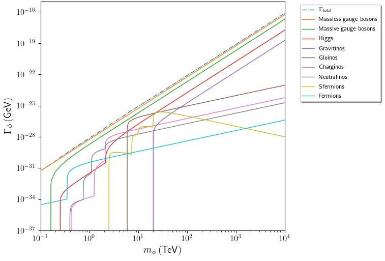
In Fig. 1, we show the modulus field partial widths versus modulus mass from 0.1 to TeV assuming the natural SUSY benchmark point in Table 2 with unsuppressed decay to gravitinos but suppressed decay to gauginos (case B1). Here, we assume all couplings equal to unity. For TeV, only decays to fermions (, etc., blue curve) and massless gauge bosons (e.g. and , orange curve) are open and GeV, corresponding to keV, so that the modulus field would decay well after BBN, which occurs beginning at MeV. As increases, decays to massive vector bosons (, , green curve) turn on at GeV, followed by decays into Higgs pairs, which turn on at GeV (red curve). This is followed by pairs (kink in blue curve) at GeV. As increases even further, decays to neutralinos (grey curve) and charginos (magenta curve) turn on around GeV. These curves show several kinks as the various electroweakino (EWino) pair decay thresholds are passed. The decay to vector boson pairs increases as as expected, but decays to gauginos are helicity suppressed and increase instead as . This asymptotic behavior also holds for as well. Decays to sfermions (yellow curve) turn on around TeV ( mode) but then decrease with increasing as , and so become hardly significant for large values of . At TeV, also turns on (brown curve), which temporarily makes a large contribution to the total width. Lastly, we see the decay to gravitinos turns on at 20 TeV (purple curve) with the partial width increasing as . This is an important threshold since gravitino production via modulus decay is negligible for and so in this regime there is no modulus-induced gravitino problem. Asymptotically, for high , then the branching fraction BF(.
The overall modulus branching fraction to SUSY particles is an important quantity, as emphasized by Gelmini and Gondolo [51]: its value contributes to the modulus-induced LSP problem. In Fig. 2, we show the modulus branching fraction into SUSY particles vs. for the same BM point in Table 2. The branching into MSSM sparticles and gravitinos is easy to compute, but the decay into Higgs pairs can also contribute depending on the heavy Higgs boson ( and ) branching fractions into MSSM particles. These BFs are model dependent, so we show an upper and a lower bound on the assuming no Higgs decay to SUSY (lower orange curve) or the upper bound with 100% Higgs decay to SUSY (blue curve). The BF can reach as high as for TeV but asymptotically can range between for TeV.

2.6.2 Case B2, :
As a second example, we show in Fig. 3 various modulus partial widths for the case B2 with chirality suppressed decays to both gauginos and gravitinos. We also assume which might occur if the Higgs fields carry PQ charge but the field doesn’t so that the modulus-Higgs operator is disallowed via the same symmetry that forbids the parameter. The modulus-matter operator may similarly be forbidden so we take . This case would then have highly suppressed decays to SUSY particles but with allowed decays to gauge bosons. From the plot, we see that for TeV, then modulus decay to SUSY particles is comparable to decay widths to SM particles. But as increases, then the helicity suppressed decays to gauginos and gravitinos sets in and these widths become increasingly suppressed compared to decays to SM particles (mainly gluon pairs).

The situation is shown more clearly in Fig. 4 where we show instead the modulus field branching fraction into gauge bosons (blue and orange curves) along with modulus branching fractions into gauginos (red, purple, and brown curves) and the branching fraction into gravitinos (green curve). As increases, the helicity suppression sets in and the branching into SUSY particles falls off sharply compared to the branching into SM particles. This case is engineered to try to avoid overproduction of neutralino dark matter and overproduction of gravitinos while possibly diluting any relics produced at temperatures . We will see shortly why this approach unfortunately fails to solve the CMP.

Further plots can be shown for cases A1 and A2 with unsuppressed moduli decays to gauginos. These cases yield always more neutralino dark matter overproduction while the total width will be roughly the same, so in the interest of simplicity, we refrain from showing these plots.
3 Constraints on and from BBN, dark matter, and gravitino overproduction: fun with temperatures
3.1 Constraints on
The evolution of the early universe in the presence of light moduli fields depends on several important temperature values.
- •
, the reheat temperature induced by inflaton decay at the end of inflation,
- •
, the temperature at which the lightest modulus field begins to oscillate,
- •
, the temperature at which modulus and radiation energy densities become equal,
- •
, the temperature at which thermally-produced WIMPs freeze out,
- •
, the temperature of radiation at the time of modulus decay,
- •
, the temperature of radiation at the time of gravitino decay and
- •
A rough picture of the evolution of the early universe can then be depicted in terms of these temperatures and related quantities such as entropy-dilution ratio (the ratio of entropy before and after modulus decay) and non-thermal dark matter production due to modulus decay. Here, we will first assume that the reheat temperature is the maximal temperature scale after inflation resulting in a radiation dominated universe at temperatures at or just below . Here, we note that such high values are at the upper bound from Buchmuller et al. (BHLR) [86, 87] where it is shown that thermal effects from GeV would destabilize the dilaton potential and cause a runaway dilaton field. We also assume the simplest scenario for reheating in the cases where that factors into the calculations (see e.g. [88]).
At temperatures with , the modulus field is effectively frozen in its value due to the preponderance of the friction term in its equation of motion:
| (17) |
The scalar potential can be approximated as a simple harmonic oscillator (SHO) form for small values. As the universe expands, the Hubble constant (where is the total energy density and is the reduced Planck mass) decreases. When , the modulus field begins to oscillate at the oscillation temperature given in Eq. (1). Specifically, if TeV (for our assumed GeV), oscillations commence during the assumed initial radiation dominance with so that
| (18) |
If, however TeV (again, for our assumed ), oscillations will begin during reheating. As scales roughly as during this era [88] where is the scale factor of the universe, we can estimate by comparing to . Noting that the reheating period is effectively matter dominated (i.e. dominated by coherent oscillations of the inflaton), we have then
| (19) |
The values of along with an assumed value of GeV are shown in Fig. 5 versus (orange curve).
At this point, the oscillating field behaves with an equation of state of matter and so the energy density of the field diminishes as due to the expansion of the universe, while diminishes as (once the reheating period has ended). Here, is the scale factor at .
The temperature of radiation/modulus energy density equality, determined by requiring , is found to be
| (20) |
At , the field begins to dominate the energy density of the universe (depicted by the green curve in Fig. 5). Before proceeding, a few comments are warranted on Eq. (20). If oscillations begin after reheating (), one would clearly expect to encounter the first case () assuming that . Since , indeed the modulus has actually begun to dominate the energy density shortly before it begins to oscillate - i.e. its energy density is so large that it will come to dominate over radiation while still being frozen by Hubble friction. However, if some mechanism can lower the expected value of , then it would be possible to encounter the second case (). In the event that oscillations begin during reheating (), note that it is actually not possible to achieve a radiation dominated universe after reheating unless - the modulus energy density is so large that reheating should lead directly to a period of early matter domination! We leave the case of initial matter domination for future work (which requires a more careful coupled Boltzmann approach to modeling the reheating period where the presence of the oscillating modulus contributes to ). However, we do not expect the main results to differ significantly from those we find here, and where appropriate adopt for consistency with initial radiation domination. Assuming again the case where and , the modulus will actually dominate over radiation during the reheating period. The modulus then falls below radiation due to the relative scalings. This briefly leads to a radiation dominated universe once reheating concludes, and the modulus quickly becomes dominant once more as radiation is no longer sourced by inflaton decay.
In any of the above cases, the modulus field then dominates the energy density of the universe until it decays at the decay temperature given by Eq. (2) which is approximately and which obviously depends on the modulus decay width discussed in the previous Section and calculated in the Appendix. We show three values of in Fig. 5 corresponding to setting all values to 0.1 (brown curve), (purple curve), and (red curve). If , then the modulus field decays after the onset of BBN, leading to destruction of the light element abundances. For the purple curve with all , then we can read off from Fig. 5 that is required to be TeV (using the MeV value, dashed grey curve). This is the traditional solution to the old CMP. We also show in Fig. 5 the thermally-produced neutralino freeze-out temperature as the magenta dashed line. For , then the relic density of neutralino dark matter will just be its thermally-produced value which for our natural SUSY benchmark point is , about a factor 10 below the measured dark matter abundance. It is worth noting however that this approximation is not necessarily valid for neutralinos produced by the decay of non-thermally produced gravitinos, which may decay at a lower temperature - we will discuss this case in the next section.

For the case where , then a further concern for the CMP is the direct overproduction of dark matter from moduli cascade decays. The initial modulus energy density is and the modulus number density is roughly . Assuming each modulus particle decays with branching fraction , and accounting for the expansion of the universe between and , we find
| (21) |
i.e. naively, the neutralinos initially inherit the modulus field number density, subject to branching ratio and expansion effects.
However, this accounting can be greatly modified if the modulus field decays at temperature and the number density exceeds the critical density above which neutralino reannihilation effects may be important [27, 28, 19]. The Boltzmann equation for the neutralino number density is given by
| (22) |
and if , then neutralinos will reannihilate after modulus decay. The Boltzmann equation, rewritten in terms of the yield variable , where is the entropy density ( for radiation) is given by
| (23) |
which, assuming is dominated by the constant term, can be easily integrated to find or
| (24) |
so that
| (25) |
i.e. the reannihilation abundance is enhanced from its TP value by a factor . The final neutralino number density is then given by
| (26) |
with where is the critical closure density and is the scaled Hubble constant. An example of the neutralino critical number density and the neutralino number density from moduli decay is shown in Fig. 6 versus for the natural SUSY benchmark point with case B1 with helicity-suppressed decay to gauginos. We take so that gravitinos do not enter the plot. Actually in this case, Fig. 6 also describes case B2 as well since all other sparticle channels are highly subdominant compared to the gauginos. The critical density increases with until whence the assumes its thermally produced value. The value of is almost always far larger than due to the huge assumed modulus field strength . Thus, we would expect from this plot that the neutralino relic density would take its non-thermally-produced reannihilation value over all allowed values of .

Provided reannihilation effects are important, the reannihilation enhancement factor can be read off from Fig. 5. Since is so large, almost always so that the neutralino relic abundance takes the reannihilation value for .
In Fig. 7, we show the resulting neutralino relic abundance from both thermal and non-thermal production versus for the natural SUSY BM point and case B1, and for the three different values of , and 10. The orange dot-dashed line shows the measured DM abundance at . We see that for the orange curve with and TeV, then neutralinos are greatly overproduced: the moduli-induced LSP overproduction problem. Depending on the values, the measured DM abundance can be achieved, but only for TeV. If the light moduli receive masses from gravity-mediated SUSY breaking, then one expects and so to avoid neutralino overproduction, one runs into a naturalness problem in that sparticles are expected in the TeV range. Such high sparticle masses would lead to a severe Little Hierarchy Problem (LHP), wherein one would be hard-pressed to understand why the weak scale is just GeV whilst sparticles that contribute to the weak scale lie in the TeV range.

3.2 Moduli-induced gravitino problem
3.2.1 Thermally-produced gravitinos: not a problem
The usual gravitino problem in supersymmetric theories has to do with overproduction of thermally produced gravitinos along with their subsequent late decays which can lead to 1. violation of BBN limits [89, 90, 91] and 2. overproduction of neutralino dark matter. These two constraints depend on the temperature at which the gravitinos decay, and on their putative thermally-produced relic abundance, had they not decayed: . The gravitino decay temperature is
| (27) |
and so we need the gravitino decay widths. These have been calculated in Kohri et al. [92] and programmed into the coupled Boltzmann computer code [21, 22] which we use. We also use the thermally-produced gravitino production rates as calculated by Pradler and Steffen [93] (see also Ref’s [94, 95]), which depends linearly on . Typically, GeV is required to avoid gravitino overproduction followed by decay to the stable LSP thus leading to dark matter overproduction and possible conflict with BBN bounds[90, 91]. For the case with a decaying light modulus, then entropy is injected during modulus decay with a dilution factor
| (28) |
For moduli fields with , then the entropy dilution is enormous since , and all thermally-produced gravitinos will be diluted to below bounds from BBN and DM overproduction. If , entropy dilution can still be enormous for larger values of since if and if . If, however, is lowered far below the Planck scale, the entropy dilution falls rapidly.
In Fig. 8, we show the would-be thermally-produced gravitino abundance (had the gravitino not decayed) vs. gravitino mass for a GeV value, right at the BHLR bound. At such high values, there is an enormous production of gravitinos in the early universe (blue curve). However, there is also enormous entropy production from light modulus decay. We show the diluted gravitino abundance by the three dashed curves for three values of , and 1000 TeV. We see that after entropy dilution, the thermally-produced gravitino abundance has dropped to tiny levels. Thus, the late-decaying modulus field has eliminated (just) the thermally produced gravitino problem. However, the moduli-induced non-thermally produced gravitino problem is yet unresolved.

3.2.2 Non-thermally produced gravitinos
Like the modulus field, there are intricate constraints from BBN on late-decaying non-thermally-produced gravitinos in the early universe. To examine these, we plot in Fig. 9 the gravitino decay temperature vs. assuming an MSSM spectrum from our natural SUSY benchmark point. From the plot, we see that the gravitino decays at temperatures below for TeV. For higher values, then the gravitino typically is safe from BBN bounds, but not from neutralino overproduction. For , then LSPs will be produced at a huge rate from gravitino decay. The neutralino reannihilation relic abundance after gravitino decay is expected to be (using a similar treatment as for moduli decays to LSPs). As can be seen in Fig. 10, the non-thermally-produced neutralino abundance from gravitino decay is enhanced by several orders of magnitude (depending on ) beyond its thermally-produced value. This is the moduli-induced, gravitino-induced LSP overproduction problem.


3.3 Overview of vs. parameter space: case B1
In Fig. 11, we display the vs. plane assuming the natural SUSY spectra (in this case, uncorrelated with or ). The region below or to the left of the lines would be excluded by or , for two choices of and 5 MeV. The region to the lower-left of the purple line could be regarded as natural if as expected in models where the modulus receives a dominant mass contribution from soft SUSY breaking. Then models with increasing values of and would become increasingly unnatural. The diagonal line would also be favored by dominant lightest modulus mass from gravity-mediated soft SUSY breaking [57]. The region to the left of the curve we would expect to have a severe moduli-induced gravitino problem. We also show curves of and 0.1 (grey dot-dashed lines at constant and constant ). Thus, all of the plane shown has a moduli-induced LSP problem except the upper-right region where very large values of and are required. The fact that almost all of the vs. plane as shown is excluded shows the severity of the CMP in the light of naturalness.

3.4 Case B2: why the CMP is still not solved
In case B2, taking ensures a highly suppressed branching fraction to SUSY final states, as seen in Fig. 12. While one might initially expect this case to allow much more parameter space due to this extreme suppression, we find that this is generally not the case. As seen in Fig. 13, the produced number density of the neutralinos from the decay of the NTP gravitinos begins roughly nine orders of magnitude above the critical value for TeV. In fact, Fig. 14 shows that the helicity suppression does not reduce the neutralino relic density to the measured until TeV. This corresponds to a suppression of ! Although the helicity suppression can technically allow for a natural gravitino mass without overproduction of non-thermal neutralinos, one then has to understand why is roughly seven orders of magnitude above . In addition, entropy dilution due to modulus decay becomes significantly less effective with such a large , and hence thermal relics can again become problematic without some other mechanism to deal with them. We would finally like to point out that inclusion of Higgs or matter superfield decays will make the issue of non-thermal overproduction worse due to the increase in while leaving the diminishing entropy dilution relatively unchanged. Indeed, it is challenging to reconcile naturalness with the CMP even in this best case scenario.


3.5 Moduli-induced baryogenesis problem
A further cosmological problem arising from weak scale moduli in the early universe pertains to baryogenesis (for some recent reviews, see e.g. Refs. [96, 97, 98]). We have seen that a late-decaying modulus field can inject an enormous amount of entropy into the early universe at temperatures MeV. Such entropy dilution of any relics present at the time of decay is problematic for many baryogenesis scenarios which occur at higher temperatures. For instance, EW baryogenesis[99] (perhaps no longer viable in a SUSY context[100]) is expected to occur at or around GeV and so any baryon asymmetry produced via this mechanism would be wiped out. Similarly, thermal leptogenesis[101] via heavy neutrino production[102] requires GeV, with conversion to a baryon asymmetry via sphaleron effects at temperatures around TeV[103]; thus, this sort of asymmetry would also likely be wiped out by radiation production from late-time modulus decay. A third mechanism– Affleck-Dine (AD) baryogenesis[104, 105] via coherent production of a baryon or lepton number carrying scalar field along a classical flat direction– can be highly efficient at producing the baryon asymmetry so that entropy dilution from late-time modulus decay can actually bring the baryon asymmetry into accord with its measured value[96]. In addition, a range of new mechanisms have been proposed which make use of the properties of the modulus decay to generate both a baryon asymmetry and the dark matter abundance. These models purport then to explain why the seemingly unrelated abundances of baryons and dark matter are comparable in the present epoch: . Starting with Thomas in 1995[106], some relevant works include [107, 108, 109, 110, 111, 112].
4 Some paths towards solving the CMP
In this Section, we discuss some of the proposed solutions to the CMP as illustrated in Fig. 11.
- •
The first solution is to conjecture that the dominant contribution to moduli masses is not from soft SUSY breaking, but rather from other possibly non-perturbative effects. Then the lightest modulus may have masses far beyond the weak scale whilst MSSM sparticles that contribute to the weak scale and are associated with naturalness have far smaller values. This issue is entangled with the issue of moduli stabilization [113], and so far can be rather speculative due to lack of experimental guidance and lack of knowledge of the details of the 6-7 dimensional compactified spaces whose properties are determined by the various moduli.
- •
- •
In DRT (Ref. [36]), Hubble-induced soft masses are invoked in the early universe but some symmetry could cause the modulus field to settle to the same minimum as in the low energy theory. Then could be small and the energy release from modulus decay could be miniscule.
- •
In Ref. [46], a late-decaying saxion field is invoked to dilute all relics. In this case, the saxion would be but one element of an axion superfield, so one would expect additional axion dark matter and additional LSPs produced from axino decay in the early universe. Plus, one would have to arrange for the saxion to not decay into SUSY particles or dark radiation [114] so that its role is solely as a source of entropy dilution of all relics at the saxion decay temperature.
- •
In Ref. [48], several specific hidden sectors are suggested to solve the moduli-induced LSP overproduction. In a hidden extension which is spontaneously broken by a pair of hidden chiral multiplets, then a hidden sector gaugino is the LSP and the MSSM LSP decays to it via portal interactions. Typical values of GeV. The annihilation cross section must be large enough to generate but then the can annihilate strongly enough into s that IDD bounds come into play. To obey IDD bounds, the typically then forms only a small fraction of the total DM abundance. Perhaps axions can make up the remainder [19]. Blinov et al. also consider a hidden with asymmetric dark matter and a non-Abelian hidden gauge group with similar conclusions: the addition of extra light hidden sector states might help evade the CMP but perhaps at the cost of implausible parameter and/or model choices.
- •
In Ref. [53, 115], Acharya et al. explain how moduli are stabilized and how exponentially suppressed scales emerge in 11-d M-theory compactified on a manifold of -holonomy (which leads to the MSSM plus moduli plus axions as the 4-d EFT). They present arguments that the lightest modulus field should have mass nearby to the gravitino mass (which sets the mass scale for scalar fields in the theory) [57] (see also Ref. [58]). Since , then the lightest modulus decay mode to gravitinos is closed and there is no moduli-induced gravitino problem. To avoid BBN constraints, then TeV and so also TeV. Since gaugino masses could be suppressed either dynamically or via symmetries compared to scalar masses, they can be much lighter: TeV. The authors initially expected AMSB-like masses for gauginos with a wino as LSP which is thermally underproduced by typically two orders of magnitude from the measured value. Then the wino abundance can be non-thermally enhanced via modulus decay to near its measured value for TeV. This basic scenario of wino DM produced from moduli decay was first introduced by Moroi and Randall [29]. Since then, the wino as a DM candidate seems ruled out due to constraints from indirect DM detection [61, 62, 63]. Acharya et al. [69] have since then explored the possibility of an inert hidden sector DM candidate which would still be allowed.
- •
Recently a landscape solution to the CMP has been proposed [116]. In that paper (which overlaps considerably with this one), the huge non-thermally produced dark matter abundance from modulus decay is noted as yielding a huge dark-matter-to-baryon ratio for which there may be anthropic limits in the multiverse: e.g. structure might appear as virialized dark matter clouds with little baryonic content [117, 118, 119, 120, 121]. Then if the values of are spread uniformly in different pocket universes (PU) within the multiverse, only those PUs with would lead to livable universes. The huge suppression of would lead to so that the neutralinos would inherit the suppressed modulus field number density which could bring the dark matter abundance into accord with measured values. The case is illustrated in Fig. 15 which we reproduce here for the convenience of the reader.

The anthropic solution to the CMP also presents a solution to the moduli-induced baryogenesis problem. Namely, with , then is highly reduced and entropy dilution of all relics can be reduced to , i.e. no entropy dilution: see Fig. 16. Then the several baryogenesis mechanisms that require become once again viable. On the other hand, there may now be no moduli-dilution of thermally-produced gravitinos. In this case, GeV may be required to avoid the thermally-produced gravitino problem[98].

5 Summary and conclusions
In this paper we have investigated the CMP with regard to 1. limits imposed by late decaying moduli which disrupt the successful predictions of BBN, 2. overproduction of gravitinos from moduli which lead to BBN violations or DM overproduction (the moduli-induced gravitino problem) and 3. non-thermal overproduction of neutralino dark matter via moduli decays (the moduli-induced LSP problem). We also confronted the CMP with expectations from SUSY naturalness, as exhibited by SUSY models with low . While the first of these can be solved by taking TeV, the second is more serious but can be solved in cases where so that moduli decay to gravitino pairs is kinematically not open. The more serious is the third of these: dark matter overproduction from moduli decays. All these issues require computing the putative moduli decay widths into MSSM particles and gravitino pairs. We perform this task including all phase space and mixing effects in the Appendix to this paper. One can then solve the moduli-induce dark matter problem by taking TeV for the case of our natural SUSY benchmark model. However, if the lightest modulus mass gains mass dominantly from SUSY breaking so that , then we would also expect sparticles up around the TeV range. This would require huge finetuning to understand why then the weak scale exists at scale GeV. We review other potential solutions to the CMP including the recent anthropic solution that could arise from the string landscape in the context of an eternally inflating multiverse[116]. We expect to address issues associated with dark radiation from moduli decay to axion-like-particles (ALPs) in a future work, as well as implementing our calculations into a coupled Boltzmann equation calculation which could include the effects of axions, saxions and axinos in addition to MSSM particles and gravitinos.
Acknowledgments
We thank L. Randall for suggesting this project more than ten years ago. This material is based upon work supported by the U.S. Department of Energy, Office of Science, Office of High Energy Physics under Award Number DE-SC-0009956 and U.S. Department of Energy (DoE) Grant DE-SC-0017647. The work of KJB was supported by the National Research Foundation of Korea (NRF) grant funded by the Korean government (NRF-2020R1C1C1012452).
Appendix A Modulus decay widths
In this Appendix, we shall use the notation and to denote the chargino and neutralino mass eigenstates of the MSSM. This alternative notation is intended to remind the reader that all mixing notation in this Appendix is given in accord with the text Weak Scale Supersymmetry: From Superfields to Scattering Events[1].
A.1 Decay into gauge fields
Here, we adopt the Moroi-Randall (MR) operator [29]
(which leads to helicity-suppressed modulus decay to gauginos (case B)). For the case of helicity-unsuppressed decay to gauginos, which occurs when fields in the gauge kinetic function obtain a SUSY breaking vev[42] (case A), then we will replace factors of in all decay width formulae for modulus to gauginos pairs (where stands for generic gaugino fields).
Expanding to the relevant terms (ignoring for now the modulino and setting as we expect SUSY breaking to primarily come from other sources), we have from [122] Eq. 6.13 (converting from mostly-plus to mostly-minus Minkowski metric):
Since we are in the Weyl basis, we can combine the spinors and the Pauli matrices into the Weyl representation of the Clifford algebra:
The term coupled to is then a surface term and will only arise in instanton corrections. We are only left with directly contributing to interactions (as expected). Changing to the Majorana representation and switching to the notation of [1], we have
where we have also made explicit the generalization to non-Abelian gauge groups. We now need to rid ourselves of the auxiliary field , for which we must first include the other relevant terms in the Lagrangian:
and so the equation of motion for becomes
where we neglect the contribution between and as it is Planck suppressed in comparison to the leading order term of the equation of motion. Note that the D-term induces an interaction between and the matter scalars. We ignore for now these interactions, as they will be 4-body decays and hence highly suppressed. There is the possible exception of a 2-body decay in the presence of a Fayet-Iliopoulos term, but we ignore that contribution as well.
Therefore, for the gauge and gaugino fields, we have the relevant Lagrangian terms
| (29) |
A.2 Modulus decay into electroweakinos
Looking at the first term of Eq. 29, we can insert the and components:
| (30) | ||||||
| (31) | ||||||
where we used the shorthand , with for and interactions, and for interactions.
This then gives us a 3-point interaction between a gaugino pair and the modulus, and a 4-point interaction between the gauge fields, a gaugino pair, and the modulus. We want to move to the mass eigenstate basis with the help of the following identities:
and
A.2.1 Relevant matrix elements and phase space formulae
Once we are in the mass eigenstate basis, there are a few general forms for the interaction. It is convenient to work out the Feynman rules, matrix elements, and phase space factors to derive general decay widths and insert the specific couplings and particles later. All of these formulae are worked out in the rest frame of the modulus.
We start with the 3-point interaction formulae. The first general interaction is of the form:
| (32) |
which corresponds to the diagram:
If we take the incoming momenta of the modulus to be , and the outgoing momenta of and to be and , respectively, we have a vertex factor of . The matrix element is then
| (33) |
Summing over outgoing spins, the squared matrix element is then
With our momenta convention, we see that , so . The final squared matrix element is then
| (34) |
As this is a 2-body decay with no angular dependence, we have the decay width immediately:
| (35) |
where we used the general formula
| (36) |
with being the combinatorial factor for identical particles ( in this case). The decay of (summing over both and final states) is then
| (37) |
A.2.2 3-point interactions
We first look at the 3-point interactions between the modulus and a gaugino pair. The last pair of 3-point interaction terms of Eq. 31 give us our neutralino interactions:
| (38) |
The corresponding matrix element is then
where and if is odd (even). The squared matrix elements for (summing over both and final states) is then,
| (39) | ||||
| (40) |
where we note that the and convention defined above simply flips the sign of the mass cross-term if one (not both) of the masses is negative, and hence we assume that all masses above are taken with their implicit absolute values. The decay widths for these processes then are:
| (41) | ||||||
| (42) | ||||||
The first 3-point interaction term of Eq. 31 then gives us our chargino interactions:
To evaluate this in the mass eigenstate basis, we see that:
where we made the definitions
| (43) | ||||
| (44) | ||||
| (45) | ||||
| (46) | ||||
| (47) | ||||
| (48) |
We therefore have the interaction terms for the charginos:
| (49) | ||||||
| (50) | ||||||
| (51) |
These have then the corresponding matrix elements
| (52) | ||||
| (53) | ||||
| (54) |
where the matrix element for is identical to . Assuming no additional contributions to these decay channels, the squared matrix elements are then
| (55) | ||||||
| (56) | ||||||
| (57) | ||||||
where we summed over both and final states for the last entry. These then have the corresponding decay widths
| (58) | ||||||
| (59) | ||||||
| (60) | ||||||
A.3 Modulus decay into electroweak vector bosons
We now look at the decay of the modulus into the electroweak vector bosons. Starting with the second term of Eq. 29, we can insert the and gauge fields:
We see that there are 3-point, 4-point, and 5-point interactions between the modulus and gauge fields.
A.3.1 Relevant matrix element formulae for electroweak vector bosons
In this section, we work out the general interactions that will be relevant for the electroweak vector bosons. All of these formulae are worked out in the rest frame of the modulus.
We start with the 3-point interaction formulae. The first general interaction is of the form:
| (61) | ||||
| (62) |
which corresponds to the diagram:
Taking the incoming momenta of the modulus to be , and the outgoing momenta of and to be and , respectively, we have a vertex factor from the first term of . Since the second interaction term is of the same form but with the exchange , we have its vertex factor of . If both vector bosons are identical, each vertex factor should be multiplied by an extra factor of 2. The associated matrix element is then
With our momenta conventions, assuming no additional contributions to this decay channel, the squared matrix element is then
and summing over polarizations (assuming both and are massive, so we use ), this becomes
In the rest frame of the modulus, we can evaluate , giving us our squared matrix element:
| (63) |
We also evaluate the squared matrix element if one of either or is massless. We’ll take to be massless (and from an Abelian group) and to be massive, where we now use for the massless boson:
The squared matrix element then is given by
| (64) |
If we now take both and to be massless, the squared matrix element is
and hence the squared matrix element is
| (65) |
For Eq’s 63, 64, and 65, again if and are identical, the entire squared matrix element must be multiplied by an additional factor of .
A.3.2 3-point interactions
We first look at the 3-point interactions between the modulus and a gauge boson pair. The relevant terms are then
Isolating the charged vector bosons, we have the interaction between the modulus and the bosons:
| (66) |
We can then evaluate the squared matrix element from Eq. 63, assuming no additional contributions to this decay channel:
| (67) |
We then have the decay width to pairs:
| (68) |
We now turn to the neutral vector bosons:
From this, we can extract the interaction:
| (69) | ||||||
The squared matrix element, assuming no other contributions to the decay, is taken from Eq. 63:
| (70) |
The decay width to pairs is then given by:
| (71) |
where we divide by an additional factor of 2 since the final state particles are indistinguishable.
The interaction follows similarly, with the interaction term:
| (72) | ||||||
which has an associated squared matrix element from Eq. 65:
| (73) |
The decay width to photon pairs is then given by:
| (74) |
where we again divide by an additional factor of 2 as the final state particles are indistinguishable.
Finally, we also need to include the interaction:
| (75) | ||||||
The corresponding matrix element from Eq. 64 is
| (76) |
Note that, as expected, if the couplings between and are equal, the interaction disappears, and the and interactions are independent of . The decay width to the state is then:
| (77) |
where we used .
A.4 Modulus decay into gluinos
The modulus decay into gluinos is given by the first term in Eq. 29:
| (78) |
A.4.1 3-point interactions
We look first at the 3-point interactions between the modulus and a gluino pair. The interaction term relevant for this process is
Since there is no symmetry breaking in the sector, we can immediately write down the matrix element to gluinos using Eq. 33:
| (79) |
and so we get the squared matrix element from Eq. 34:
| (80) |
The additional factor of comes from summing over the color indices, as while the gluinos are a color octet, specific color charges are of no interest for this work. The computation of the decay width, including a factor for identical final state particles, gives
| (81) |
A.5 Modulus decay into gluons
We can get the modulus decay into gluons from the second term in Eq. 29:
| (82) | ||||||
A.5.1 Relevant matrix element formulae for gluons
In this section, we work out the general interactions that will be relevant for the gluons. All of these formulae are worked out in the rest frame of the modulus.
We start with the 3-point interaction formulae. The first general interaction is of the form:
| (83) | ||||
| (84) |
which corresponds to the diagram:
Taking the incoming momenta of the modulus to be , and the outgoing momenta of and to be and , respectively, we have a vertex factor from the first term of . Since the second interaction term is of the same form but with the exchange , we have its vertex factor of . Because the gluons have identical color charge, each vertex factor should be multiplied by an extra factor of 2. The associated matrix element is then
Since we’re dealing with bosons associated with a non-Abelian symmetry, we have to be careful about the polarization sums here. We first note that only the transverse polarizations are physical, and since the gluons are back-to-back in the rest frame of the modulus, we must have . On summing over the polarizations, we have also where we defined assuming is propagating in the direction.
This simplifies the physical matrix element to
and the squared matrix element becomes
which matches our expectation based on the matrix element.
A.5.2 3-point interactions
We look first at the 3-point interactions between the modulus and gluons. The interaction term relevant for this process is
This corresponds to a squared matrix element
| (85) |
where, again, the extra factor of 8 comes from summing over all possible final gluons. This gives us a total decay width of
| (86) |
where we divide by an extra factor of 2 as the final state particles are indistinguishable.
A.6 Decay into Higgs fields
We have the interaction term for the modulus-Higgs sector [29]
We focus first on the subset of terms and obtain the remaining results by the substitutions and . Expanding as per Ref. [1] Eqs. 5.34 and 5.37, we need to first evaluate the superspace integral (noting that we disregard the modulino and the terms):
Using the Grassmann variable identities, integrating some terms by parts, leveraging the Majorana nature of (taking e.g. ), and rearranging, we can rewrite this as
This Lagrangian contains some redundancies in the scalar interactions, so we need to exploit surface term identities to simplify this expression. We can take the total derivatives:
and, on ignoring the surface terms, we arrive at the following identities:
We also realize that the entire second line of the Lagrangian vanishes, due to the separate chirality of the spinors in each interaction. Hence, the modulus should only interact with the scalar components of each of the Higgs superfields. This then allows us to rewrite the Lagrangian as
Finally, we separate the fields into their real and imaginary components:
| (87) |
We can write down the result for the charged Higgs sectors by the aforementioned replacements and :
| (88) |
A.6.1 Relevant matrix element formulae for Higgs bosons
In this section, we work out the general interactions that will be relevant for the Higgs bosons. All of these formulae are worked out in the rest frame of the modulus.
We start with the 3-point interaction formulae. The first general interaction is of the form:
| (89) |
which corresponds to the diagram:
Taking the incoming momenta of the modulus to be , and the outgoing momenta of and to be and , respectively, we have a vertex factor of . The corresponding matrix element is then
which must be also multiplied by an additional factor of 2 if . Assuming no additional contributions to this decay channel, the squared matrix element is
| (90) |
which, again, must be multiplied by an additional factor of 4 if .
A.6.2 Neutral Higgs interactions
We first start with the neutral Higgs sector interactions. We write down the term for the real component of the modulus interacting with the neutral Higgs from 87:
We then move to the mass eigenstate basis with the following transformations:
This gives us a Lagrangian of the form
We can extract from this the interaction between the modulus and the light Higgs pair:
| (91) |
The corresponding squared matrix element from Eq. 90 is then
| (92) |
This gives us the decay width to light Higgs pairs:
| (93) |
where we divide by an additional factor of 2 due to the final state particles being indistinguishable.
Likewise, the interaction between the modulus, the light Higgs, and the heavy Higgs is given by
| (94) |
which has a squared matrix element of
| (95) |
The decay width for this process is then given by
| (96) |
Finally, the interaction between the modulus and the heavy Higgs pair is:
| (97) |
which has corresponding squared matrix element
| (98) |
The decay width to heavy Higgs pairs is then given by:
| (99) |
where we again divide by an additional factor of 2 since the final state particles are indistinguishable.
In the CP-odd sector, we have the decay to the pseudoscalar Higgs given by
| (100) |
The corresponding squared matrix element is
| (101) |
The decay width to pseudoscalar Higgs pairs is then:
| (102) |
where we once again divide by an additional factor of 2 for indistinguishable final state particles.
We can similarly write down the term for the imaginary component of the modulus interacting with the neutral Higgs from Eq. 87:
and move to the mass eigenstate basis:
We extract the interaction between the modulus, the light Higgs, and the pseudoscalar Higgs:
| (103) |
The corresponding squared matrix element for this decay channel is
| (104) |
which then has a decay width of
| (105) |
Likewise, the interaction between the modulus, the heavy Higgs, and the pseudoscalar Higgs is given by:
| (106) |
which has a corresponding matrix element
| (107) |
The decay width is given by:
| (108) |
A.6.3 Charged Higgs interactions
We find the charged Higgs interactions similarly to the neutral Higgs interactions. Taking the interactions with the real component of the modulus, we have from Eq. 88 the term
We move to the mass eigenstate basis with the following transformations:
which gives us the following Lagrangian:
| (109) |
We can now extract the interaction between the modulus and the charged Higgs pair:
| (110) |
which has, from Eq. 90, the squared matrix element
| (111) |
The decay width to charged Higgs pairs is given by
| (112) |
We follow similarly for the interactions with the imaginary component of the modulus. From Eq. 88, we have the term
We again move to the mass basis with the same transformations as above:
| (113) |
A.7 Decay into matter fields
We have the operator relevant for fermion interactions (Ref. [29])
Ignoring the modulino, we have then the following interaction Lagrangian:
This expression has some redundancies in the scalar components, and we can exploit surface terms to simplify this Lagrangian. Taking the total derivative and distributing differentials in various permutations (so as to end up with surface terms that can be neglected), we have:
Putting these together, we arrive at the following identity which allows us to replace the terms with mixed differentials:
This then allows us to rewrite the Lagrangian as:
| (114) |
We neglect the couplings to the fields for now, as they will be 4-body decay terms.
A.7.1 Relevant matrix element formulae for sfermions
In this section, we work out the general interactions that will be relevant for the sfermions. All of these formulae are worked out in the rest frame of the modulus.
We start with the 3-point interaction formulae. The first general interaction is of the form:
| (115) |
which corresponds to the diagram:
Since we have a real scalar decaying to complex scalars, the tree-level matrix element is simply the vertex factor. The vertex factor here is then and hence the matrix element is
| (116) |
Note that if the interaction Lagrangian has a second derivative on the term instead of , the mass in the matrix element will simply be relabeled to correspond to the field with the second derivative coupling.
A.7.2 Relevant matrix element formulae for fermions
In this section, we work out the general interactions that will be relevant for the fermions. All of these formulae are worked out in the rest frame of the modulus.
We start with the 3-point interaction formulae. The first general interaction is of the form:
| (117) | ||||
| (118) |
which corresponds to the diagram:
Taking the incoming momenta of the modulus to be , and the outgoing momenta of and to be and , respectively, we have a vertex factor of . The matrix element is then
The second general interaction is rather similar:
| (119) | ||||
| (120) |
which corresponds to the same diagram as above, albeit with a different vertex factor. Taking again the incoming momenta of the modulus to be , and the outgoing momenta of and to be and , respectively, we have a vertex factor of . The matrix element is then
There are similar interactions as well, which interchange . These interactions have identical matrix elements as above, but with the replacement .
It is worthwhile to also work out the combination:
| (121) |
The matrix element for this combination reduces to
| (122) |
If there are no other contributions to this decay process, we can evaluate the squared matrix element for the combination above:
Summing over outgoing spins, we have then:
Noting that (with our assigned momenta), we have , in the rest frame we have then . Therefore, the final squared matrix element in the rest frame of the modulus is
| (123) |
Finally, we should work out the combination:
| (124) |
The matrix element for this decay channel is then (keeping the same momenta conventions)
| (125) |
Again assuming no other contributions to this channel, we can evaluate the squared matrix element for this combination (making the definitions and ):
Summing over spins, we get
Again, we can substitute and plug back in and to get the final squared matrix element in the rest frame of the modulus:
| (126) |
A.8 Modulus decay into squarks
We take the term from Eq. 114
Starting with the right-handed quark singlets (note the abuse of notation, where the subscript refers to either right-handed or real part based on the context), we have
and similarly for the down-type quark singlets. This is then approximately the mass eigenstate Lagrangian for the right-handed squarks as we neglect mixing effects.
Using the mixing matrix for
we then have the following Lagrangian in the mass eigenstate basis for the 3rd squark generations where mixing is relevant:
We now evaluate the left-handed quark doublets. This gives us
where the coupling is the same between the up and down type left-handed squarks (within the same generation). This is approximately the mass eigenstate Lagrangian for the left-handed squarks.
Using the left-handed mixing similar to before for , we then have the following Lagrangian in the mass eigenstate basis for 3rd generation squarks:
The left and right handed 3rd generation squarks then combine to give the following interactions with :
| (127) | ||||
| (128) | ||||
| (129) |
with corresponding matrix elements
| (130) | ||||
| (131) | ||||
| (132) |
Assuming there are no additional contributions to the decay channels, we can write down the squared matrix elements:
| (133) | ||||
| (134) | ||||
| (135) |
These processes then have the associated decay widths:
| (136) | ||||
| (137) | ||||
| (138) |
Note that we do not divide by an additional factor of 2 here, as these final states are complex scalars and hence are distinguishable due to their associated charge.
The interactions with are given by:
| (139) | ||||||
| (140) | ||||||
| (141) |
Note that the extra factor of in the interactions with takes care of the field interactions which are of the form (and hence are purely imaginary). Furthermore, note that all tree-level matrix elements are 0 for the decay of to the squarks.
The interactions with the squarks are identical, with the replacements , , , however the coupling is unchanged (as left-handed components belong to the same multiplet). For completeness, we also recap the interactions for the first two generations. The left-handed squarks are given by
| (142) | ||||||
| (143) |
with corresponding matrix elements
| (144) | ||||
| (145) |
and squared matrix element
| (146) |
where if and if . The decay width to the left-handed squarks is then given by
| (147) |
The right-handed squarks are given by (again, calling attention to the abuse of notation by using the subscript to refer to either real part or right-handed based on context):
| (148) | ||||||
| (149) |
with corresponding matrix elements
| (150) | ||||
| (151) |
and squared matrix element
| (152) |
for up-type squarks, with the replacement for down-type squarks. The decay width to the right-handed (up-type) squarks is then given by
| (153) |
noting the replacement for also the down-type right-handed squarks.
A.9 Modulus decay into sleptons
The modulus decays into sleptons follow from the same term from Eq. 114 as the squarks. We simply write down the interaction terms by direct analogy.
Since the neutrino masses have been neglected, the sneutrinos have no mixing and hence the interaction terms are given by
| (154) | ||||||
| (155) |
which have corresponding matrix elements
| (156) | ||||
| (157) |
and squared matrix element
| (158) |
where . The decay width to sneutrino pairs is then given by
| (159) |
The first two generations of selectron-type sleptons follow:
| (160) | ||||||
| (161) | ||||||
| (162) | ||||||
| (163) |
which have corresponding matrix elements
| (164) | ||||
| (165) | ||||
| (166) | ||||
| (167) |
and squared matrix elements
| (168) | ||||
| (169) |
where here . The decay widths for these processes are then given by
| (170) | ||||
| (171) |
For the staus, we assume mixing of the same form as for the stops, so the resulting interaction terms with are
| (172) | ||||||
| (173) | ||||||
| (174) |
with corresponding matrix elements
| (175) | ||||
| (176) | ||||
| (177) |
The squared matrix elements are then
| (178) | ||||
| (179) | ||||
| (180) |
The associated decay widths for these processes are then given by
| (181) | ||||
| (182) | ||||
| (183) |
The interactions with are given by
| (184) | ||||||
| (185) | ||||||
| (186) |
Again, all tree-level matrix elements vanish for the decay of to the sleptons.
A.10 Modulus decay into quarks
We take the term from Eq. 114
where in the last line, we use the Majorana spinor identity , which makes the interaction with vanish.
We can then write the full interaction piece for a single generation of both up and down type quarks:
To progress further in terms of the Dirac quark fields, we will need to use a few tricks, namely:
and insert factors of . Upon evaluating this out and leveraging some Majorana bilinear identities, we can rewrite an interaction piece as
Hence, for the up-type quarks, we have the full interaction piece involving the Dirac fields
| (187) |
The down-type quarks can be gotten directly with the replacements and . Note that, unless , the different chiral components of the quark fields interact slightly differently. The associated matrix element is then (from Eq. A.7.2, and using the subscript to distinguish the spinor components of the up-quark field)
| (188) |
(where the associated matrix element for the down-type quarks can be retrieved from the replacements above). Assuming no additional contributions to the decay channel, we can write down the squared matrix element from Eq. 126:
| (189) |
The decay width to up-type quark pairs is then given by
| (190) |
For the sake of completeness, we write the associated squared matrix element for the down-type quarks:
| (191) |
The decay width to down-type quark pairs is then given by
| (192) |
A.11 Modulus decay into leptons
We proceed to calculate the widths to leptons similarly to the quarks. We can immediately write down the interactions:
We can again write down the Dirac fields as
and, inserting factors of , we have
Hence, the charged leptons have the full interaction piece involving the Dirac fields
| (193) |
The associated matrix element can then be written down from Eq. A.7.2:
| (194) |
Assuming no other contributions to the decay channel, we can write down the squared matrix element from Eq. 126:
| (195) |
The decay width to charged lepton pairs is then given by
| (196) |
A.12 Modulus decay to gravitino pairs
Nakamura and Yamaguchi (NY) Ref. [42] consider the case of particular models which lead to helicity-unsuppressed modulus decay to gravitinos (case 1):
| (200) |
where is defined in terms of the Kähler function as . The dimensionless constant is then model-dependent depending on the form of the Kähler function but is expected to be of order unity. We have appended a phase space factor to the formula of NY. While the NY formula is technically valid in the high energy limit where gravitino decay is dominantly to goldstino components, we adopt this form even in the lower energy limit. This form for modulus decay to gravitino pairs was also obtained by Endo et al. Ref. [44].
Another possibility is that for other forms of the Kähler function [47], the modulus decay to gravitinos is helicity suppressed (case 2). In that case, we use the above formula but with the replacement .
References
- [1] H. Baer, X. Tata, Weak scale supersymmetry: From superfields to scattering events, Cambridge University Press, 2006.
- [2] H. Baer, V. Barger, S. Salam, D. Sengupta, K. Sinha, Status of weak scale supersymmetry after LHC Run 2 and ton-scale noble liquid WIMP searches, Eur. Phys. J. ST 229 (21) (2020) 3085–3141. arXiv:2002.03013, doi:10.1140/epjst/e2020-000020-x.
- [3] U. Amaldi, W. de Boer, H. Furstenau, Comparison of grand unified theories with electroweak and strong coupling constants measured at LEP, Phys. Lett. B 260 (1991) 447–455. doi:10.1016/0370-2693(91)91641-8.
- [4] L. E. Ibanez, G. G. Ross, SU(2)-L x U(1) Symmetry Breaking as a Radiative Effect of Supersymmetry Breaking in Guts, Phys. Lett. B 110 (1982) 215–220. doi:10.1016/0370-2693(82)91239-4.
- [5] P. Slavich, et al., Higgs-mass predictions in the MSSM and beyond, Eur. Phys. J. C 81 (5) (2021) 450. arXiv:2012.15629, doi:10.1140/epjc/s10052-021-09198-2.
- [6] S. Heinemeyer, W. Hollik, G. Weiglein, L. Zeune, Implications of LHC search results on the W boson mass prediction in the MSSM, JHEP 12 (2013) 084. arXiv:1311.1663, doi:10.1007/JHEP12(2013)084.
- [7] H. Baer, V. Barger, D. Mickelson, How conventional measures overestimate electroweak fine-tuning in supersymmetric theory, Phys. Rev. D 88 (9) (2013) 095013. arXiv:1309.2984, doi:10.1103/PhysRevD.88.095013.
- [8] A. Mustafayev, X. Tata, Supersymmetry, Naturalness, and Light Higgsinos, Indian J. Phys. 88 (2014) 991–1004. arXiv:1404.1386, doi:10.1007/s12648-014-0504-8.
- [9] H. Baer, V. Barger, D. Mickelson, M. Padeffke-Kirkland, SUSY models under siege: LHC constraints and electroweak fine-tuning, Phys. Rev. D 89 (11) (2014) 115019. arXiv:1404.2277, doi:10.1103/PhysRevD.89.115019.
- [10] H. Baer, V. Barger, P. Huang, A. Mustafayev, X. Tata, Radiative natural SUSY with a 125 GeV Higgs boson, Phys. Rev. Lett. 109 (2012) 161802. arXiv:1207.3343, doi:10.1103/PhysRevLett.109.161802.
- [11] H. Baer, V. Barger, P. Huang, D. Mickelson, A. Mustafayev, X. Tata, Radiative natural supersymmetry: Reconciling electroweak fine-tuning and the Higgs boson mass, Phys. Rev. D 87 (11) (2013) 115028. arXiv:1212.2655, doi:10.1103/PhysRevD.87.115028.
- [12] H. Baer, A. D. Box, H. Summy, Neutralino versus axion/axino cold dark matter in the 19 parameter SUGRA model, JHEP 10 (2010) 023. arXiv:1005.2215, doi:10.1007/JHEP10(2010)023.
- [13] K. Griest, D. Seckel, Three exceptions in the calculation of relic abundances, Phys. Rev. D 43 (1991) 3191–3203. doi:10.1103/PhysRevD.43.3191.
- [14] J. R. Ellis, T. Falk, K. A. Olive, Neutralino - Stau coannihilation and the cosmological upper limit on the mass of the lightest supersymmetric particle, Phys. Lett. B 444 (1998) 367–372. arXiv:hep-ph/9810360, doi:10.1016/S0370-2693(98)01392-6.
- [15] H. Baer, M. Brhlik, M. A. Diaz, J. Ferrandis, P. Mercadante, P. Quintana, X. Tata, Yukawa unified supersymmetric SO(10) model: Cosmology, rare decays and collider searches, Phys. Rev. D 63 (2000) 015007. arXiv:hep-ph/0005027, doi:10.1103/PhysRevD.63.015007.
- [16] J. R. Ellis, T. Falk, G. Ganis, K. A. Olive, M. Srednicki, The CMSSM parameter space at large tan beta, Phys. Lett. B 510 (2001) 236–246. arXiv:hep-ph/0102098, doi:10.1016/S0370-2693(01)00541-X.
- [17] N. Arkani-Hamed, A. Delgado, G. F. Giudice, The Well-tempered neutralino, Nucl. Phys. B 741 (2006) 108–130. arXiv:hep-ph/0601041, doi:10.1016/j.nuclphysb.2006.02.010.
- [18] H. Baer, A. Mustafayev, E.-K. Park, X. Tata, Target dark matter detection rates in models with a well-tempered neutralino, JCAP 01 (2007) 017. arXiv:hep-ph/0611387, doi:10.1088/1475-7516/2007/01/017.
- [19] H. Baer, A. Lessa, S. Rajagopalan, W. Sreethawong, Mixed axion/neutralino cold dark matter in supersymmetric models, JCAP 06 (2011) 031. arXiv:1103.5413, doi:10.1088/1475-7516/2011/06/031.
- [20] K. J. Bae, H. Baer, E. J. Chun, Mainly axion cold dark matter from natural supersymmetry, Phys. Rev. D 89 (3) (2014) 031701. arXiv:1309.0519, doi:10.1103/PhysRevD.89.031701.
- [21] H. Baer, A. Lessa, W. Sreethawong, Coupled Boltzmann calculation of mixed axion/neutralino cold dark matter production in the early universe, JCAP 01 (2012) 036. arXiv:1110.2491, doi:10.1088/1475-7516/2012/01/036.
- [22] K. J. Bae, H. Baer, A. Lessa, H. Serce, Coupled Boltzmann computation of mixed axion neutralino dark matter in the SUSY DFSZ axion model, JCAP 10 (2014) 082. arXiv:1406.4138, doi:10.1088/1475-7516/2014/10/082.
- [23] S. Kachru, R. Kallosh, A. D. Linde, S. P. Trivedi, De Sitter vacua in string theory, Phys. Rev. D 68 (2003) 046005. arXiv:hep-th/0301240, doi:10.1103/PhysRevD.68.046005.
- [24] K. Choi, A. Falkowski, H. P. Nilles, M. Olechowski, Soft supersymmetry breaking in KKLT flux compactification, Nucl. Phys. B 718 (2005) 113–133. arXiv:hep-th/0503216, doi:10.1016/j.nuclphysb.2005.04.032.
- [25] V. Balasubramanian, P. Berglund, J. P. Conlon, F. Quevedo, Systematics of moduli stabilisation in Calabi-Yau flux compactifications, JHEP 03 (2005) 007. arXiv:hep-th/0502058, doi:10.1088/1126-6708/2005/03/007.
- [26] R. Blumenhagen, J. P. Conlon, S. Krippendorf, S. Moster, F. Quevedo, SUSY Breaking in Local String/F-Theory Models, JHEP 09 (2009) 007. arXiv:0906.3297, doi:10.1088/1126-6708/2009/09/007.
- [27] G. F. Giudice, E. W. Kolb, A. Riotto, Largest temperature of the radiation era and its cosmological implications, Phys. Rev. D 64 (2001) 023508. arXiv:hep-ph/0005123, doi:10.1103/PhysRevD.64.023508.
- [28] K.-Y. Choi, J. E. Kim, H. M. Lee, O. Seto, Neutralino dark matter from heavy axino decay, Phys. Rev. D 77 (2008) 123501. arXiv:0801.0491, doi:10.1103/PhysRevD.77.123501.
- [29] T. Moroi, L. Randall, Wino cold dark matter from anomaly mediated SUSY breaking, Nucl. Phys. B 570 (2000) 455–472. arXiv:hep-ph/9906527, doi:10.1016/S0550-3213(99)00748-8.
- [30] G. D. Coughlan, W. Fischler, E. W. Kolb, S. Raby, G. G. Ross, Cosmological Problems for the Polonyi Potential, Phys. Lett. B 131 (1983) 59–64. doi:10.1016/0370-2693(83)91091-2.
- [31] M. Dine, W. Fischler, D. Nemeschansky, Solution of the Entropy Crisis of Supersymmetric Theories, Phys. Lett. B 136 (1984) 169–174. doi:10.1016/0370-2693(84)91174-2.
- [32] T. Banks, D. B. Kaplan, A. E. Nelson, Cosmological implications of dynamical supersymmetry breaking, Phys. Rev. D 49 (1994) 779–787. arXiv:hep-ph/9308292, doi:10.1103/PhysRevD.49.779.
- [33] B. de Carlos, J. A. Casas, F. Quevedo, E. Roulet, Model independent properties and cosmological implications of the dilaton and moduli sectors of 4-d strings, Phys. Lett. B 318 (1993) 447–456. arXiv:hep-ph/9308325, doi:10.1016/0370-2693(93)91538-X.
- [34] L. Randall, S. D. Thomas, Solving the cosmological moduli problem with weak scale inflation, Nucl. Phys. B 449 (1995) 229–247. arXiv:hep-ph/9407248, doi:10.1016/0550-3213(95)00228-K.
- [35] T. Banks, M. Berkooz, P. J. Steinhardt, The Cosmological moduli problem, supersymmetry breaking, and stability in postinflationary cosmology, Phys. Rev. D 52 (1995) 705–716. arXiv:hep-th/9501053, doi:10.1103/PhysRevD.52.705.
- [36] M. Dine, L. Randall, S. D. Thomas, Supersymmetry breaking in the early universe, Phys. Rev. Lett. 75 (1995) 398–401. arXiv:hep-ph/9503303, doi:10.1103/PhysRevLett.75.398.
- [37] G. R. Dvali, Inflation versus the cosmological moduli problem (3 1995). arXiv:hep-ph/9503259.
- [38] D. H. Lyth, E. D. Stewart, Thermal inflation and the moduli problem, Phys. Rev. D 53 (1996) 1784–1798. arXiv:hep-ph/9510204, doi:10.1103/PhysRevD.53.1784.
- [39] M. Hashimoto, K. I. Izawa, M. Yamaguchi, T. Yanagida, Gravitino overproduction through moduli decay, Prog. Theor. Phys. 100 (1998) 395–398. arXiv:hep-ph/9804411, doi:10.1143/PTP.100.395.
- [40] K. Kohri, M. Yamaguchi, J. Yokoyama, Production and dilution of gravitinos by modulus decay, Phys. Rev. D 70 (2004) 043522. arXiv:hep-ph/0403043, doi:10.1103/PhysRevD.70.043522.
- [41] K. Kohri, M. Yamaguchi, J. Yokoyama, Neutralino dark matter from heavy gravitino decay, Phys. Rev. D 72 (2005) 083510. arXiv:hep-ph/0502211, doi:10.1103/PhysRevD.72.083510.
- [42] S. Nakamura, M. Yamaguchi, Gravitino production from heavy moduli decay and cosmological moduli problem revived, Phys. Lett. B 638 (2006) 389–395. arXiv:hep-ph/0602081, doi:10.1016/j.physletb.2006.05.078.
- [43] T. Asaka, S. Nakamura, M. Yamaguchi, Gravitinos from heavy scalar decay, Phys. Rev. D 74 (2006) 023520. arXiv:hep-ph/0604132, doi:10.1103/PhysRevD.74.023520.
- [44] M. Endo, K. Hamaguchi, F. Takahashi, Moduli-induced gravitino problem, Phys. Rev. Lett. 96 (2006) 211301. arXiv:hep-ph/0602061, doi:10.1103/PhysRevLett.96.211301.
- [45] M. Nagai, K. Nakayama, Nonthermal dark matter in mirage mediation, Phys. Rev. D 76 (2007) 123501. arXiv:0709.3918, doi:10.1103/PhysRevD.76.123501.
- [46] M. Endo, F. Takahashi, Non-thermal Production of Dark Matter from Late-Decaying Scalar Field at Intermediate Scale, Phys. Rev. D 74 (2006) 063502. arXiv:hep-ph/0606075, doi:10.1103/PhysRevD.74.063502.
- [47] M. Dine, R. Kitano, A. Morisse, Y. Shirman, Moduli decays and gravitinos, Phys. Rev. D 73 (2006) 123518. arXiv:hep-ph/0604140, doi:10.1103/PhysRevD.73.123518.
- [48] N. Blinov, J. Kozaczuk, A. Menon, D. E. Morrissey, Confronting the moduli-induced lightest-superpartner problem, Phys. Rev. D 91 (3) (2015) 035026. arXiv:1409.1222, doi:10.1103/PhysRevD.91.035026.
- [49] L. Randall, R. Sundrum, Out of this world supersymmetry breaking, Nucl. Phys. B 557 (1999) 79–118. arXiv:hep-th/9810155, doi:10.1016/S0550-3213(99)00359-4.
- [50] C. Pallis, Massive particle decay and cold dark matter abundance, Astropart. Phys. 21 (2004) 689–702. arXiv:hep-ph/0402033, doi:10.1016/j.astropartphys.2004.05.006.
- [51] G. B. Gelmini, P. Gondolo, Neutralino with the right cold dark matter abundance in (almost) any supersymmetric model, Phys. Rev. D 74 (2006) 023510. arXiv:hep-ph/0602230, doi:10.1103/PhysRevD.74.023510.
- [52] G. Gelmini, P. Gondolo, A. Soldatenko, C. E. Yaguna, The Effect of a late decaying scalar on the neutralino relic density, Phys. Rev. D 74 (2006) 083514. arXiv:hep-ph/0605016, doi:10.1103/PhysRevD.74.083514.
- [53] B. S. Acharya, K. Bobkov, G. Kane, P. Kumar, D. Vaman, An M theory Solution to the Hierarchy Problem, Phys. Rev. Lett. 97 (2006) 191601. arXiv:hep-th/0606262, doi:10.1103/PhysRevLett.97.191601.
- [54] B. S. Acharya, K. Bobkov, G. L. Kane, J. Shao, P. Kumar, The G(2)-MSSM: An M Theory motivated model of Particle Physics, Phys. Rev. D 78 (2008) 065038. arXiv:0801.0478, doi:10.1103/PhysRevD.78.065038.
- [55] B. S. Acharya, P. Kumar, K. Bobkov, G. Kane, J. Shao, S. Watson, Non-thermal Dark Matter and the Moduli Problem in String Frameworks, JHEP 06 (2008) 064. arXiv:0804.0863, doi:10.1088/1126-6708/2008/06/064.
- [56] B. S. Acharya, G. Kane, S. Watson, P. Kumar, A Non-thermal WIMP Miracle, Phys. Rev. D 80 (2009) 083529. arXiv:0908.2430, doi:10.1103/PhysRevD.80.083529.
- [57] B. S. Acharya, G. Kane, E. Kuflik, Bounds on scalar masses in theories of moduli stabilization, Int. J. Mod. Phys. A 29 (2014) 1450073. arXiv:1006.3272, doi:10.1142/S0217751X14500730.
- [58] F. Denef, M. R. Douglas, Distributions of nonsupersymmetric flux vacua, JHEP 03 (2005) 061. arXiv:hep-th/0411183, doi:10.1088/1126-6708/2005/03/061.
- [59] R. Allahverdi, M. Cicoli, B. Dutta, K. Sinha, Nonthermal dark matter in string compactifications, Phys. Rev. D 88 (9) (2013) 095015. arXiv:1307.5086, doi:10.1103/PhysRevD.88.095015.
- [60] G. Kane, K. Sinha, S. Watson, Cosmological Moduli and the Post-Inflationary Universe: A Critical Review, Int. J. Mod. Phys. D 24 (08) (2015) 1530022. arXiv:1502.07746, doi:10.1142/S0218271815300220.
- [61] T. Cohen, M. Lisanti, A. Pierce, T. R. Slatyer, Wino Dark Matter Under Siege, JCAP 10 (2013) 061. arXiv:1307.4082, doi:10.1088/1475-7516/2013/10/061.
- [62] J. Fan, M. Reece, In Wino Veritas? Indirect Searches Shed Light on Neutralino Dark Matter, JHEP 10 (2013) 124. arXiv:1307.4400, doi:10.1007/JHEP10(2013)124.
- [63] H. Baer, V. Barger, H. Serce, SUSY under siege from direct and indirect WIMP detection experiments, Phys. Rev. D 94 (11) (2016) 115019. arXiv:1609.06735, doi:10.1103/PhysRevD.94.115019.
- [64] H. Baer, V. Barger, D. Sengupta, X. Tata, Is natural higgsino-only dark matter excluded?, Eur. Phys. J. C 78 (10) (2018) 838. arXiv:1803.11210, doi:10.1140/epjc/s10052-018-6306-y.
- [65] C. Han, Higgsino Dark Matter in a Non-Standard History of the Universe, Phys. Lett. B 798 (2019) 134997. arXiv:1907.09235, doi:10.1016/j.physletb.2019.134997.
- [66] M. Drees, F. Hajkarim, Dark Matter Production in an Early Matter Dominated Era, JCAP 02 (2018) 057. arXiv:1711.05007, doi:10.1088/1475-7516/2018/02/057.
- [67] M. Drees, F. Hajkarim, Neutralino Dark Matter in Scenarios with Early Matter Domination, JHEP 12 (2018) 042. arXiv:1808.05706, doi:10.1007/JHEP12(2018)042.
- [68] L. Aparicio, M. Cicoli, B. Dutta, F. Muia, F. Quevedo, Light Higgsino Dark Matter from Non-thermal Cosmology, JHEP 11 (2016) 038. arXiv:1607.00004, doi:10.1007/JHEP11(2016)038.
- [69] B. S. Acharya, S. A. R. Ellis, G. L. Kane, B. D. Nelson, M. J. Perry, The lightest visible-sector supersymmetric particle is likely to be unstable, Phys. Rev. Lett. 117 (2016) 181802. arXiv:1604.05320, doi:10.1103/PhysRevLett.117.181802.
- [70] B. S. Acharya, S. A. R. Ellis, G. L. Kane, B. D. Nelson, M. Perry, Categorisation and Detection of Dark Matter Candidates from String/M-theory Hidden Sectors, JHEP 09 (2018) 130. arXiv:1707.04530, doi:10.1007/JHEP09(2018)130.
- [71] K. R. Dienes, J. Kost, B. Thomas, A Tale of Two Timescales: Mixing, Mass Generation, and Phase Transitions in the Early Universe, Phys. Rev. D 93 (4) (2016) 043540. arXiv:1509.00470, doi:10.1103/PhysRevD.93.043540.
- [72] K. R. Dienes, J. Kost, B. Thomas, A new approach to the cosmological moduli problem, AIP Conf. Proc. 1743 (1) (2016) 020003. doi:10.1063/1.4953270.
- [73] B. S. Acharya, M. Dhuria, D. Ghosh, A. Maharana, F. Muia, Cosmology in the presence of multiple light moduli, JCAP 11 (2019) 035. arXiv:1906.03025, doi:10.1088/1475-7516/2019/11/035.
- [74] L. Susskind, The Anthropic landscape of string theory (2003) 247–266arXiv:hep-th/0302219.
- [75] L. Susskind, Supersymmetry breaking in the anthropic landscape, in: From Fields to Strings: Circumnavigating Theoretical Physics: A Conference in Tribute to Ian Kogan, 2004, pp. 1745–1749. arXiv:hep-th/0405189, doi:10.1142/9789812775344-0040.
- [76] M. R. Douglas, Statistical analysis of the supersymmetry breaking scale (5 2004). arXiv:hep-th/0405279.
- [77] N. Arkani-Hamed, S. Dimopoulos, S. Kachru, Predictive landscapes and new physics at a TeV (1 2005). arXiv:hep-th/0501082.
- [78] V. Agrawal, S. M. Barr, J. F. Donoghue, D. Seckel, Anthropic considerations in multiple domain theories and the scale of electroweak symmetry breaking, Phys. Rev. Lett. 80 (1998) 1822–1825. arXiv:hep-ph/9801253, doi:10.1103/PhysRevLett.80.1822.
- [79] G. F. Giudice, A. Masiero, A Natural Solution to the mu Problem in Supergravity Theories, Phys. Lett. B 206 (1988) 480–484. doi:10.1016/0370-2693(88)91613-9.
- [80] K. J. Bae, H. Baer, V. Barger, D. Sengupta, Revisiting the SUSY problem and its solutions in the LHC era, Phys. Rev. D 99 (11) (2019) 115027. arXiv:1902.10748, doi:10.1103/PhysRevD.99.115027.
- [81] H. Baer, A. Mustafayev, S. Profumo, A. Belyaev, X. Tata, Direct, indirect and collider detection of neutralino dark matter in SUSY models with non-universal Higgs masses, JHEP 07 (2005) 065. arXiv:hep-ph/0504001, doi:10.1088/1126-6708/2005/07/065.
- [82] F. E. Paige, S. D. Protopopescu, H. Baer, X. Tata, ISAJET 7.69: A Monte Carlo event generator for pp, anti-p p, and e+e- reactions (12 2003). arXiv:hep-ph/0312045.
- [83] M. Kawasaki, K. Kohri, N. Sugiyama, Cosmological constraints on late time entropy production, Phys. Rev. Lett. 82 (1999) 4168. arXiv:astro-ph/9811437, doi:10.1103/PhysRevLett.82.4168.
- [84] M. Kawasaki, K. Kohri, N. Sugiyama, MeV scale reheating temperature and thermalization of neutrino background, Phys. Rev. D 62 (2000) 023506. arXiv:astro-ph/0002127, doi:10.1103/PhysRevD.62.023506.
- [85] T. Hasegawa, N. Hiroshima, K. Kohri, R. S. L. Hansen, T. Tram, S. Hannestad, MeV-scale reheating temperature and thermalization of oscillating neutrinos by radiative and hadronic decays of massive particles, JCAP 12 (2019) 012. arXiv:1908.10189, doi:10.1088/1475-7516/2019/12/012.
- [86] W. Buchmuller, K. Hamaguchi, O. Lebedev, M. Ratz, Dilaton destabilization at high temperature, Nucl. Phys. B 699 (2004) 292–308. arXiv:hep-th/0404168, doi:10.1016/j.nuclphysb.2004.08.031.
- [87] W. Buchmuller, K. Hamaguchi, O. Lebedev, M. Ratz, Maximal temperature in flux compactifications, JCAP 01 (2005) 004. arXiv:hep-th/0411109, doi:10.1088/1475-7516/2005/01/004.
- [88] E. W. Kolb, M. S. Turner, The Early Universe, Vol. 69, 1990.
- [89] K. Jedamzik, Big bang nucleosynthesis constraints on hadronically and electromagnetically decaying relic neutral particles, Phys. Rev. D 74 (2006) 103509. arXiv:hep-ph/0604251, doi:10.1103/PhysRevD.74.103509.
- [90] M. Kawasaki, K. Kohri, T. Moroi, A. Yotsuyanagi, Big-Bang Nucleosynthesis and Gravitino, Phys. Rev. D 78 (2008) 065011. arXiv:0804.3745, doi:10.1103/PhysRevD.78.065011.
- [91] M. Kawasaki, K. Kohri, T. Moroi, Y. Takaesu, Revisiting Big-Bang Nucleosynthesis Constraints on Long-Lived Decaying Particles, Phys. Rev. D 97 (2) (2018) 023502. arXiv:1709.01211, doi:10.1103/PhysRevD.97.023502.
- [92] K. Kohri, T. Moroi, A. Yotsuyanagi, Big-bang nucleosynthesis with unstable gravitino and upper bound on the reheating temperature, Phys. Rev. D 73 (2006) 123511. arXiv:hep-ph/0507245, doi:10.1103/PhysRevD.73.123511.
- [93] J. Pradler, F. D. Steffen, Thermal gravitino production and collider tests of leptogenesis, Phys. Rev. D 75 (2007) 023509. arXiv:hep-ph/0608344, doi:10.1103/PhysRevD.75.023509.
- [94] V. S. Rychkov, A. Strumia, Thermal production of gravitinos, Phys. Rev. D 75 (2007) 075011. arXiv:hep-ph/0701104, doi:10.1103/PhysRevD.75.075011.
- [95] H. Eberl, I. D. Gialamas, V. C. Spanos, Gravitino thermal production revisited, Phys. Rev. D 103 (7) (2021) 075025. arXiv:2010.14621, doi:10.1103/PhysRevD.103.075025.
- [96] M. Dine, A. Kusenko, The Origin of the matter - antimatter asymmetry, Rev. Mod. Phys. 76 (2003) 1. arXiv:hep-ph/0303065, doi:10.1103/RevModPhys.76.1.
- [97] K. Enqvist, A. Mazumdar, Cosmological consequences of MSSM flat directions, Phys. Rept. 380 (2003) 99–234. arXiv:hep-ph/0209244, doi:10.1016/S0370-1573(03)00119-4.
- [98] K. J. Bae, H. Baer, H. Serce, Y.-F. Zhang, Leptogenesis scenarios for natural SUSY with mixed axion-higgsino dark matter, JCAP 01 (2016) 012. arXiv:1510.00724, doi:10.1088/1475-7516/2016/01/012.
- [99] D. E. Morrissey, M. J. Ramsey-Musolf, Electroweak baryogenesis, New J. Phys. 14 (2012) 125003. arXiv:1206.2942, doi:10.1088/1367-2630/14/12/125003.
- [100] M. Quiros, M. Seco, Electroweak baryogenesis in the MSSM, Nucl. Phys. B Proc. Suppl. 81 (2000) 63–70. arXiv:hep-ph/9903274, doi:10.1016/S0920-5632(99)00860-9.
- [101] W. Buchmuller, R. D. Peccei, T. Yanagida, Leptogenesis as the origin of matter, Ann. Rev. Nucl. Part. Sci. 55 (2005) 311–355. arXiv:hep-ph/0502169, doi:10.1146/annurev.nucl.55.090704.151558.
- [102] M. Fukugita, T. Yanagida, Baryogenesis Without Grand Unification, Phys. Lett. B 174 (1986) 45–47. doi:10.1016/0370-2693(86)91126-3.
- [103] V. A. Kuzmin, V. A. Rubakov, M. E. Shaposhnikov, On the Anomalous Electroweak Baryon Number Nonconservation in the Early Universe, Phys. Lett. B 155 (1985) 36. doi:10.1016/0370-2693(85)91028-7.
- [104] I. Affleck, M. Dine, A New Mechanism for Baryogenesis, Nucl. Phys. B 249 (1985) 361–380. doi:10.1016/0550-3213(85)90021-5.
- [105] M. Dine, L. Randall, S. D. Thomas, Baryogenesis from flat directions of the supersymmetric standard model, Nucl. Phys. B 458 (1996) 291–326. arXiv:hep-ph/9507453, doi:10.1016/0550-3213(95)00538-2.
- [106] S. D. Thomas, Baryons and dark matter from the late decay of a supersymmetric condensate, Phys. Lett. B 356 (1995) 256–263. arXiv:hep-ph/9506274, doi:10.1016/0370-2693(95)00772-D.
- [107] R. Kitano, H. Murayama, M. Ratz, Unified origin of baryons and dark matter, Phys. Lett. B 669 (2008) 145–149. arXiv:0807.4313, doi:10.1016/j.physletb.2008.09.049.
- [108] R. Allahverdi, B. Dutta, K. Sinha, Baryogenesis and Late-Decaying Moduli, Phys. Rev. D 82 (2010) 035004. arXiv:1005.2804, doi:10.1103/PhysRevD.82.035004.
- [109] R. Allahverdi, B. Dutta, K. Sinha, Cladogenesis: Baryon-Dark Matter Coincidence from Branchings in Moduli Decay, Phys. Rev. D 83 (2011) 083502. arXiv:1011.1286, doi:10.1103/PhysRevD.83.083502.
- [110] K. Ishiwata, K. S. Jeong, F. Takahashi, Moduli-induced Baryogenesis, JHEP 02 (2014) 062. arXiv:1312.0954, doi:10.1007/JHEP02(2014)062.
- [111] M. Dhuria, C. Hati, U. Sarkar, Moduli induced cogenesis of baryon asymmetry and dark matter, Phys. Lett. B 756 (2016) 376–383. arXiv:1508.04144, doi:10.1016/j.physletb.2016.03.018.
- [112] G. Kane, M. W. Winkler, Baryogenesis from a Modulus Dominated Universe, JCAP 02 (2020) 019. arXiv:1909.04705, doi:10.1088/1475-7516/2020/02/019.
- [113] M. Bose, M. Dine, P. Draper, Moduli or Not, Phys. Rev. D 88 (2013) 023533. arXiv:1305.1066, doi:10.1103/PhysRevD.88.023533.
- [114] K. J. Bae, H. Baer, A. Lessa, Dark Radiation Constraints on Mixed Axion/Neutralino Dark Matter, JCAP 04 (2013) 041. arXiv:1301.7428, doi:10.1088/1475-7516/2013/04/041.
- [115] B. S. Acharya, K. Bobkov, G. L. Kane, P. Kumar, J. Shao, Explaining the Electroweak Scale and Stabilizing Moduli in M Theory, Phys. Rev. D 76 (2007) 126010. arXiv:hep-th/0701034, doi:10.1103/PhysRevD.76.126010.
- [116] H. Baer, V. Barger, R. W. Deal, An anthropic solution to the cosmological moduli problem (11 2021). arXiv:2111.05971.
- [117] A. D. Linde, Inflation and Axion Cosmology, Phys. Lett. B 201 (1988) 437–439. doi:10.1016/0370-2693(88)90597-7.
- [118] F. Wilczek, A Model of anthropic reasoning, addressing the dark to ordinary matter coincidence (2004) 151–162arXiv:hep-ph/0408167.
- [119] M. Tegmark, A. Aguirre, M. Rees, F. Wilczek, Dimensionless constants, cosmology and other dark matters, Phys. Rev. D 73 (2006) 023505. arXiv:astro-ph/0511774, doi:10.1103/PhysRevD.73.023505.
- [120] B. Freivogel, Anthropic Explanation of the Dark Matter Abundance, JCAP 03 (2010) 021. arXiv:0810.0703, doi:10.1088/1475-7516/2010/03/021.
- [121] R. Bousso, L. Hall, Why Comparable? A Multiverse Explanation of the Dark Matter-Baryon Coincidence, Phys. Rev. D 88 (2013) 063503. arXiv:1304.6407, doi:10.1103/PhysRevD.88.063503.
- [122] J. Wess, J. Bagger, Supersymmetry and supergravity, Princeton University Press, Princeton, NJ, USA, 1992.