Doubly robust estimators for generalizing treatment effects on survival outcomes from randomized controlled trials to a target population
Abstract
In the presence of heterogeneity between the randomized controlled trial (RCT) participants and the target population, evaluating the treatment effect solely based on the RCT often leads to biased quantification of the real-world treatment effect. To address the problem of lack of generalizability for the treatment effect estimated by the RCT sample, we leverage observational studies with large samples that are representative of the target population. This paper concerns evaluating treatment effects on survival outcomes for a target population and considers a broad class of estimands that are functionals of treatment-specific survival functions, including differences in survival probability and restricted mean survival times. Motivated by two intuitive but distinct approaches, i.e., imputation based on survival outcome regression and weighting based on inverse probability of sampling, censoring, and treatment assignment, we propose a semiparametric estimator through the guidance of the efficient influence function. The proposed estimator is doubly robust in the sense that it is consistent for the target population estimands if either the survival model or the weighting model is correctly specified, and is locally efficient when both are correct. In addition, as an alternative to parametric estimation, we employ the nonparametric method of sieves for flexible and robust estimation of the nuisance functions and show that the resulting estimator retains the root- consistency and efficiency, the so-called rate-double robustness. Simulation studies confirm the theoretical properties of the proposed estimator and show it outperforms competitors. We apply the proposed method to estimate the effect of adjuvant chemotherapy on survival in patients with early-stage resected non-small lung cancer.
Keywords: Causal inference, Data integration, Generalizability, Survival analysis, Semiparametric efficiency.
1 Introduction
In clinical trials or biomedical studies, time-to-event or survival endpoints, such as the time from treatment initiation to death, have been commonly used to evaluate the treatment effect. When estimating treatment effect, randomized controlled trials (RCTs) are regarded as the gold standard since randomization reduces the effect of confounding variables. However, RCTs often suffer from a lack of generalizability or external validity. Specifically, due to restrictive inclusion and exclusion criteria for enrollment or additional concerns from patients and physicians, RCTs often don’t recruit enough participants that represent the real-world patient population, resulting in the covariate distribution of the RCT sample being different from that of the target real-world population. In the presence of such heterogeneity, evaluating the treatment effect based solely on the RCT sample leads to biased quantification of the real-world treatment effect. As a complement of the RCT sample, observational studies have been widely used in comparative effectiveness research, as large samples that are representative of the target population can be studied at a relatively low cost.
Several recent works have proposed integrative methods to generalize findings from the RCT to the target population by leveraging observational studies (Cole and Stuart 2010; Tipton 2013; Hartman et al. 2015; Dahabreh et al. 2019; Lee et al. 2021). Most existing methods focus on directly modeling the probability of participating in the trial, i.e., the sampling score which is analogous to the treatment propensity score. A widely used approach involves inverse probability of sampling weighting (Cole and Stuart 2010; Stuart et al. 2011, IPSW;), which can be used to estimate weight-adjusted survival curves (Cole and Hernán 2004; Pan and Schaubel 2008). However, these IPSW-based estimators are unstable under extreme sampling scores. Alternatively, Lee et al. 2021 proposed calibration weighting that enforces covariate balance between the RCT and observational study without explicitly modeling the sampling score. Recently, Colnet et al. 2020 provided a comprehensive review of various novel methods combining complementary features of RCTs and observational studies. However, most of these methods focus on continuous and binary outcomes, and generalization of the findings from RCTs for survival outcomes to the target population is less actively studied.
In this paper, we consider a broad class of estimands defined as a functional of treatment-specific survival functions, including differences in survival probability at landmark times and restricted mean survival time (RMST). Various estimators can be constructed to adjust for the unrepresentativeness or selection bias of the RCT sample. One approach relies on fitting conditional survival outcome models and then averaging over the covariate distribution of the observational sample, similar to Chen and Tsiatis 2001. Another common approach is to use weighting (Cole and Hernán 2004; Wei and Schaubel 2008) to adjust for the imbalance between the RCT sample and the observational sample. Instead of direct modeling of sampling score as in IPSW, one can consider the more stable approach that calibrates covariate distributions between the RCT and the observational sample (Lee et al. 2021). Motivated by these two intuitive but distinct approaches, we propose improved estimators for survival outcomes under the guidance of the efficient influence function (EIF), which involve survival outcome regression and weighting based on inverse probability of treatment, censoring, and sampling, simultaneously. The proposed estimator is doubly robust in the sense that it is consistent for the target population estimand if either the survival model or the weighting model is correctly specified, and is locally efficient when both are correct. In addition, to cope with possible misspecification of nuisance functions, we consider the method of sieves (Chen 2007), which adds great flexibility and robustness to the proposed estimators, meanwhile retaining the root- consistency.
The remainder of the paper is organized as follows. In Section 2, we formalize the basic causal inference framework for survival outcomes. In Section 3, we introduce two direct estimators based on identification formulas, and in Section 4, we propose improved estimators and describe the corresponding asymptotic properties. The finite sample performance of the proposed estimators is assessed via simulation studies in Section 5. Applying the proposed estimators, we analyze the effect of adjuvant chemotherapy on the survival of lung cancer patients with data from an RCT and an observational study in Section 6. Section 7 presents the discussion and concluding remarks. All proofs are provided in the Appendix.
2 Estimands, Observed Data, and Assumptions
Suppose we are interested in comparing the effectiveness of two treatments. Let be the binary treatment assignment, A . Following the potential outcomes framework (Rubin 1974; Rubin 1986), let be the potential survival time if a subject received the treatment , and and be the corresponding survival and hazard functions, i.e., and . Under the proportional hazards assumption, a widely used measure to characterize the treatment effect is hazard ratio (HR), i.e., being a constant. However, the interpretation of HRs is challenging especially when the proportionality assumption is violated (Hernán 2010; Trinquart et al. 2016).
Alternatively, we define the average treatment effect (ATE) measure as a function of treatment-specific survival curves, where is a pre-specified constant. This formulation of the ATE includes a broad class of estimands that are favored in survival analysis (Yang et al. 2020). For example, is a simple survival difference at a fixed time , and is the restricted mean survival time (RMST) difference up to . The ratio of restricted mean time loss (RMTL) and the difference of the median survival can also be represented with the appropriate choice of .
Under the Stable Unit Treatment Value Assumption, the survival time is the realization of the potential outcomes, i.e., . Let be the censoring time. In the presence of right censoring, the survival time is not observed for all subjects; instead, we observe and where represents the minimum of two values, and is an indicator function. Let be a -dimensional vector of pre-treatment covariates. Also, let denotes the binary indicator of RCT participation, and let denotes the binary indicator of observational study participation. We consider a super-population framework assuming that an RCT sample of size and an observational sample of size are sampled from the target population. From the RCT sample, we observe from independent and identically distributed subjects. For the observational sample, it is common that only the covariates information is available, i.e., from independent and identically distributed subjects. The sampling mechanism and data structure are illustrated in Figure 1. We assume independence between the RCT and the observational sample, which holds if two separate studies are conducted by independent researchers, the target patient population is sufficiently large, or the patients are enrolled in two separate time periods.
Let be the treatment-specific conditional survival curves for . Also, define the treatment propensity score and the sampling score . In order to identify the ATE from the observed data, we make the following assumptions:
Assumption 1 (Ignorability and positivity of trial treatment assignment)
1
(i) ; and (ii) with probability .
Assumption 2 (Conditional survival exchangeablity and positivity of trial participation)
(i) ; and (ii) with probability .
Assumption 3 (Noninformative censoring conditional on covariates and treatment)
1
, which also implies .
Assumptions 1–3 are not testable in general and their plausibility should be justified based on subject matter knowledge in practice. Assumption 1 holds in the RCT by default. Assumption 2 (i) is plausible if all information related to the trial participation and the outcome is captured in the data at hand. This assumption is weaker than the ignorablility of the trial participation assumption, i.e., . The relationship between Assumption 2 (i) and its stronger version is analogous to that described in Dahabreh et al. 2019 in the context of continuous and binary outcomes. Assumption 2 (ii) implies that the absence of patient characteristics that prevent from participating in the trial (Lee et al. 2021). Assumption 3 is commonly made in survival analysis (Chen and Tsiatis 2001; Zhang and Schaubel 2012b; Zhang et al. 2019). This assumption is weaker than the conditional independence assumption of the censoring and survival time given only on the treatment (Zhang and Schaubel 2012a).
The covariate distribution of the RCT sample may not be representative of that of the target population due to restrictive trial enrollment criteria, but the covariate distribution of the observational sample is often representative of due to the real-world data collection mechanism. In particular, if the observational sample is a simple random sample of the target population, then . More generally, the observational sample can be selected under complex sampling designs. To accommodate such scenarios, we can define as the known design weight for the observational sample.
Assumption 4 (The known design weight for the observational sample)
1
The observational sample design weight is known.
Assumption 4 is commonly assumed in the survey sampling literature. Based on Assumption 4, the design-weighted observational sample is representative of the target population. In an observational study with simple random sampling, , where is the target population size.
Under the above assumptions, the ATE , or sufficiently, are identified based on the observed data. We consider two identification formulas. Let , and define the conditional censoring model . One identification formula is based on the conditional survival curves, i.e.,
| (1) |
which can be called the OS-design-weighted G-computation formula. Note that if the population covariate distribution is available, is the G-computation formula for . The other identification formula is based on the inverse probability weighting (IPW) approach for the marginal survival curves, i.e.,
| (2) |
for . The two identification formulas in (1) and (2) motivate the estimators in the following section, depending on different components of the observed data likelihood.
3 Two Direct Estimators based on Identification Formulas
3.1 Outcome Regression
Based on the identification formula (1), the treatment-specific conditional survival curve can be modeled and fitted based on the observed data, e.g., using the widely used Cox regression model for the survival outcome. A treatment-specific conditional hazard function at time given covariate is defined as
| (3) |
where is a treatment-specific baseline hazard function, for . Following standard survival analysis techniques, can be estimated as a solution to the partial likelihood score equation, and the baseline cumulative hazard can be estimated by the Breslow 1974 estimator,
where , , and . The survival model in (3) does not imply that the marginal HR of the potential survival outcomes under and , i.e., , is a constant and thus is not restrictive. Other survival models can be considered, including the additive hazards model (Lin and Ying 1995; Aalen 1989).
Chen and Tsiatis 2001 proposed a method that accounts for imbalances between treatment groups by first estimating the conditional treatment effect given and then averaging the effect over across both treatment groups. A similar approach can be applied to balance the covariate distribution between the RCT sample and the observational sample by first estimating the treatment-specific survival curve conditional on under model (3), i.e., , and then applying the design-weighted averaging over . The resulting outcome regression (OR) estimator of the marginal treatment-effect survival curve is
| (4) |
for , and the corresponding ATE estimator is defined as . The OR estimator is consistent when the survival model (3) is correctly specified.
3.2 Inverse Probability and Calibration Weighting
We can construct the estimator of the marginal treatment-specific survival curve based on the identification formula in (2) that involves sampling score, treatment propensity score, and censoring probability. This approach can be viewed as a combination of IPSW, inverse probability of treatment weighting (IPTW), and inverse probability of censoring weighting (IPCW). The weighting estimator requires positing models for the three probabilities and estimating them.
First, we consider the estimation of the sampling score. As the covariate distribution of the RCT sample is different from that of the target population in general, the estimated ATE based only on the RCT sample can be biased. A widely used approach to account for this selection bias is IPSW, i.e., weighting the RCT sample by the inverse probability of trial participation over that of observational study participation, to adjust for differences in covariate distribution between the trial sample and the population. Specifically, can be modeled as where . One can plug in for in (2) using the common logistic regression model. However, the IPSW method requires the sampling score model to be correctly specified; it also could be highly unstable if is close to zero for some .
Instead of direct estimating the sampling scores, Lee et al. 2021 proposed the calibration weighting approach to reduce the selection bias in the trial-based estimator, which is analogous to the entropy balancing method by Hainmueller 2012 and more stable than the IPSW method. The basic idea is that subjects in the RCT sample are calibrated to the observational sample, so that after calibration, the covariate distribution of the RCT sample empirically matches that of the target population. The calibration weighting approach is based on the idea that for any , the following identity hold,
| (5) |
where is a function of to be calibrated, e.g., the moments or any nonlinear transformations.
The calibration weights are obtained by solving the optimization problem
| (6) | ||||
| subject to |
where . The last constraint is the empirical representation of (5), where is a consistent estimator of from the observational sample. Minimizing the negative entropy function of the calibration weights in (6) enforces the weights to be as close to one another as possible, which reduces the variability due to heterogeneous weights. Using the Lagrange multiplier , the objective function of this convex optimization problem becomes . The estimated calibration weights are , where solves
| (7) |
Under the loglinear sampling score model, the calibration weights from the objective function (6) have the same functional form as inverse probability of sampling score weights asymptotically, resulting in the direct correspondence between the calibration weight and the sampling score in that , as (Lee et al. 2021). Following that, we posit the loglinear sampling score model,
| (8) |
Lee et al. 2021 showed that is equivalent to , where . Accordingly, in the rest of the paper, we represent the calibration weights using , i.e., . If one considers a logistic sampling score model instead, then other objective functions can be used, such as , that corresponds to the weights with the same functional form as the inverse to a logistic probability of sampling (Zhao 2019; Josey et al. 2020). However, the loglinear regression model in (8) is close to the logistic regression model when the proportion of the RCT sample in the target population is small.
With respect to treatment assignment, is generally known for RCTs. However, several authors suggested estimating the treatment propensity score for the RCTs in order to increase the efficiency and account for the chance of imbalance of prognostic variables (Williamson et al. 2014; Colantuoni and Rosenblum 2015, e.g.,). We choose a logistic regression model for the treatment propensity score,
| (9) |
and define . Estimating the propensity scores also broadens the scope of the current paper to allow the generalization of the observational study. Even though this paper focuses on generalizing the trial findings where we only require a two-way balancing between the RCT and observational study, a three-way balancing approach between the treated, the controlled, and the observational sample (e.g., (Chan et al. 2016)) can be useful to generalize the findings from the observational study to its larger population with the estimation of .
Moreover, in order to account for right censoring , we posit Cox proportional hazards model with conditional hazard
| (10) |
where the standard techniques as for the survival model in (3) can be used to estimate and .
4 Improved Estimators
4.1 Efficient Influence Function
Let be one copy of the vector of observed variables. The OR estimator specified in (4) and the CW estimator specified in (11) use different components of the likelihood function . Specifically, the OR estimator is based on modeling for , and the CW estimator is based on modeling , , and for . These estimators are singly robust in that they are consistent only under the correct survival outcome regression model or the correct weighting models. A vast number of estimators can be constructed by combining these two estimators. In general, the question becomes how to obtain the most efficient estimator. Our approach is to derive the EIF (Tsiatis 2006) of to construct semiparametrically efficient estimators. Such estimators also gain robustness to model misspecification as we show later.
We consider a class of influence functions of regular asymptotically linear (RAL) estimators of the treatment-specific survival curve . Define and . Following Tsiatis 2006, the class of observed data influence functions includes
| (12) |
for arbitrary functions , and , where is a Martingale with , and is a cumulative hazard for censoring for . The last three terms in (12) are mean-zero functions. According to the semiparametric theory (Tsiatis 2006), the EIF is the influence function in (12) with the smallest variance. The EIF can be derived by projecting the first term of (12) onto the orthogonal complement of the tangent space spanned by the scores of the nuisance functions, i.e., the last three terms. The RAL estimator with the EIF is a semiparametrically efficient estimator. The following theorem gives the EIF in the class of influence functions (12), with the proof given in the Appendix B.1.
Many common treatment effect estimands are functionals of the treatment-specific survival curves, including the survival difference at a fixed time , the difference of RMSTs, the ratio of RMTLs, and the difference of th quantile of survivals. Their EIFs can be expressed in the form of a combination of weighted integrals of the EIF for treatment specific survival curves (Yang et al. 2020). To be specific, the EIF for is
| (14) |
for some functions that (see Appendix A for details). We limit our interest to the estimands with such form of the EIF, which covers the broad class of estimators that are favored in survival analysis.
4.2 Augmented Calibration Weighting Estimator
Motivated by Theorem 1, under the survival model in (3) and the weighting models specified in (8)–(10), we propose the following augmented CW (ACW) estimator of the treatment-specific survival curve,
| (15) |
In addition, following the technique by Zhang and Schaubel 2012a that represents the marginal cumulative hazard function by estimating the denominator and the numerator separately, we propose another ACW estimator,
| (16) |
where
estimates . Although and are asymptotically equivalent, simulation studies show that has better finite-sample performance. The proposed ACW estimators are similar to the estimators developed by Zhang and Schaubel 2012b and Zhang et al. 2019. The difference between the proposed and their method is discussed in Section 7.
Similar to Yang et al. 2020, we consider an asymptotic linear characterization of the ATE estimator for both ACW1 and ACW2 estimators. That is, under mild regularity conditions,
| (17) |
for bounded variation functions in (14). Under the asymptotic linear characterization, has the influence function (see Appendix B.2 for the proof).
Toward this end, the following theorem shows the local efficiency and asymptotic properties of the proposed ACW estimators of the ATE, i.e., and .
Theorem 2
Under Assumptions 1–4, if either the survival model in (3) is correctly specified or the weighting models, i.e., the sampling score model (8), the treatment propensity score model (9), and the censoring model (10), are correctly specified, under regularity conditions, and are consistent for , and and are asymptotically normal with mean zero and variance and . Moreover, if all working models in (3) and (8)–(10) are correctly specified, and are locally efficient, i.e., as .
The proof of Theorem 2 and details of and are provided in the Appendix B.3. For a straightforward procedure of variance estimation, a nonparametric bootstrap method can be used. Specifically, we draw bootstrap samples from both the RCT and the observational sample respectively, and then for each resampled pair, we obtain a replicate of the ACW estimator; the sample variance of the bootstrap replicates is the variance of the ACW estimator.
The proposed ACW estimators depend on the parametric estimation of nuisance functions. Alternatively, we can consider a flexible nonparametric approach without the parametric assumption, which is often unrealistic in complex problems in practice. The asymptotic behavior of the ACW estimators with the nonparametric estimation of nuisance functions can be characterized by the empirical process perspective. Suppose that the posited nuisance models are consistent, i.e., , , and , , for . Also, suppose that the weighting functions , , and are bounded away from zero. Then, we have the effect of the estimated nuisance functions in bounded above by up to a multiplicative constant, where is a true measure such that and is norm. If each term of the bound is of rate then the effect of nuisance function estimations are asymptotically negligible. This statement is formalized in the following theorem.
Theorem 3
Suppose Assumptions 1–4 hold. Let be general semiparametric and nonparametric models for and , , be general semiparametric models for , , and , respectively, for . Suppose the following conditions hold:
- (C1)
, , , ;
- (C2)
for some ;
- (C3)
,
,
Then, and are consistent estimators for and achieve semiparametric efficiency.
4.3 Robust Estimation using the Method of Sieves with Penalization
For a robust estimation of the ATE under possibly misspecified working models, we adopt the method of sieves (Grenander 1981; Geman and Hwang 1982) which enables flexible data-adaptive estimation of the survival curves and probability weights with root-n consistency (Chen 2007). We construct the sieves using the linear spans of power series (Newey 1997), but other basis functions such as Fourier series or splines are applicable. Specifically, for a -dimensional vector of non-negative integers , we consider a -vector sieve basis functions , where with non-decreasing in , i.e., . Under standard regularity conditions, the sieves approximation results in a consistent estimation of the survival curves and weighting probabilities with large (see Lee et al. 2021, supporting information). To facilitate the stable estimation and to control the variability of the estimators with large , we consider the penalized estimation of the nuisance functions.
For the sampling score model , the penalized sieves estimation is based on the dual problem of calibration that solves the estimating equation in (7). Following the penalized estimating equation approach (Johnson et al. 2008; Wang et al. 2012; Yang et al. 2020), we solve
for , where is the element-wise product of and . We define and specify to be the popular SCAD penalty function (Fan and Li 2001), but different penalty functions such as adaptive lasso (Zou 2006) or the minimax concave penalty (Zhang 2010) are also applicable. For the SCAD penalty, we have , for , with following the literature and the tuning parameter selected by cross validation.
For penalized sieves estimation of the survival outcome model , the standard penalization technique for the Cox PH model was used based on the partial likelihood. Specifically, we estimate by solving
where is the set of indices of the events, is the set of indices of the patients at risk at time , with denotes the distinct event time, and is the SCAD penalty, for . The penalized sieves estimation of the censoring model can be adopted by analogy. Lastly, for the penalized sieves estimation of the treatment propensity score model , we use the standard penalization approach for the binary data using the logit link with the SCAD penalty.
Under regularity conditions specified in Fan and Li 2001 and Lee et al. 2021, the penalized sieve estimators of the nuisance functions possess oracle properties and satisfy two conditions in Theorem 3. Thus, the resulting ACW estimators using the method of sieves achieve the root-n consistency and semiparametric efficiency.
5 Simulation Studies
In this section, we conduct simulation studies to evaluate the finite-sample performance of the proposed estimators. We consider the target population of size and covariates , where each is generated from and truncated at and to satisfy regularity conditions. An RCT sample of size is selected from a hypothetical RCT eligible population with size . From the remaining observational study population, we randomly select a sample of size .
We consider the difference in RMST as the ATE, i.e., , where we choose . We compare the proposed CW and the ACW estimators with four other methods, the Naive estimator based only on the RCT sample, the ZS estimator, i.e., the estimator proposed by Zhang and Schaubel 2012b based only on the RCT sample, the IPSW estimator using the normalized IPSW weight in (11), and the OR estimator specified in (4). For the ACW estimators, in addition to the original covariate vector , we consider the penalized sieve estimation with calibration variables , i.e., the extension of the basis functions in to its 2nd-order power series including all two-way interactions and quadratic terms. We use (S) to indicate the method of sieves. To assess the performance of these estimators under model misspecification, we consider four scenarios where i) all four models in (3) and (8)–(10) are correct, ii) only the survival outcome model (3) is correct, iii) the outcome model is incorrect but the other three weighting models (8)–(10) are correct, iv) all four models are incorrect. Details of estimators and specification of the four working models when they are correctly/incorrectly specified are listed in Table 1.
| Models | Correctly specified | Incorrectly specified | |
|---|---|---|---|
| O | |||
| S | |||
| A | 0.5 | ||
| C | |||
| Estimators | Details | ||
| Naive | , | ||
| where | |||
| ZS | The denominator of the estimator proposed by Zhang and Schaubel 2012b | ||
| OR | , where is defined by (4) | ||
| IPSW | where | ||
| CW | where is defined by (11) | ||
| ACW1 | where is defined by (15) with | ||
| ACW2 | where is defined by (16) with | ||
| ACW1(S) | The penalized ACW1 estimator using the method of sieves with | ||
| ACW2(S) | The penalized ACW2 estimator using the method of sieves with | ||
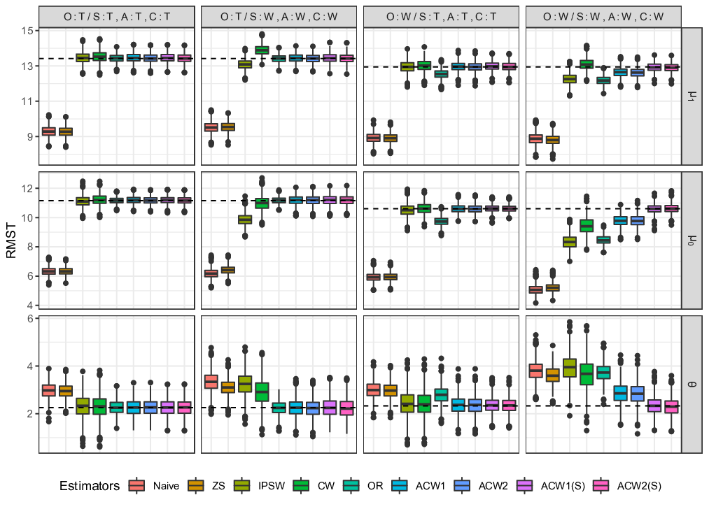
Table 2 and Figure 2 summarize the results based on 1000 Monte Carlo replications. The bootstrap variance estimation was used for all estimators with . When all models are correctly specified, the Naive and ZS estimators which are based only on the RCT sample show biased estimations of the ATE due to the selection bias in the RCT sample. The OR, IPSW, CW, and ACW estimators correct that bias by leveraging the observational sample covariates. The ACW estimators were found to be more efficient than other unbiased IPW estimators. Even though the variance of the OR estimator is smaller, it is biased when the outcome model is incorrectly specified. The CW and IPSW estimators are biased when the sampling score model is not correctly specified. The proposed ACW estimators are double robust when either the outcome model or the other three models are correctly specified. In Scenario 4 where both the outcome model and the weighting models are misspecified, the ACW estimator using the penalized sieve estimation, i.e., ACW1(S) and ACW2(S), is still unbiased. The efficiency of the ACW1(S) and ACW2(S) estimators are comparable to that of the ACW1 and ACW2 estimators in Scenario 1 and 2. In Scenario 3 and 4 where the outcome model is incorrect, using the method of sieves gains efficiency. The ACW2 and ACW2(S) estimators were found to be more consistent than the ACW1 and ACW1(S) estimators in a finite sample.
| BIAS | ESE | RSE(%) | CP(%) | |||||||||
|---|---|---|---|---|---|---|---|---|---|---|---|---|
| Estimator | ||||||||||||
| Scenario 1: O:T / S:T, A:T, C:T | ||||||||||||
| Naive | -4.12 | -4.83 | 0.71 | 0.30 | 0.28 | 0.33 | 7.44 | 3.91 | 4.97 | 0.0 | 0.0 | 39.0 |
| ZS | -4.14 | -4.83 | 0.69 | 0.29 | 0.26 | 0.30 | 7.12 | 2.13 | 4.65 | 0.0 | 0.0 | 34.2 |
| IPSW | 0.04 | -0.04 | 0.08 | 0.32 | 0.38 | 0.49 | 2.33 | -0.14 | 2.01 | 93.9 | 94.7 | 93.3 |
| CW | 0.11 | 0.06 | 0.05 | 0.32 | 0.37 | 0.50 | 2.57 | 1.57 | 2.29 | 92.4 | 93.9 | 93.7 |
| OR | 0.02 | 0.01 | 0.01 | 0.22 | 0.23 | 0.30 | 1.45 | -2.59 | 1.48 | 94.7 | 95.3 | 95.0 |
| ACW1 | 0.05 | 0.04 | 0.00 | 0.25 | 0.26 | 0.35 | 2.14 | -1.60 | 1.54 | 93.4 | 93.9 | 94.4 |
| ACW2 | 0.02 | 0.02 | 0.00 | 0.25 | 0.26 | 0.35 | 2.27 | -0.31 | 2.56 | 94.0 | 94.5 | 94.4 |
| ACW1(S) | 0.05 | 0.04 | 0.00 | 0.25 | 0.26 | 0.34 | 1.17 | -2.46 | -0.19 | 93.4 | 93.7 | 94.4 |
| ACW2(S) | 0.02 | 0.02 | 0.00 | 0.25 | 0.26 | 0.35 | 1.76 | -0.98 | 1.42 | 93.9 | 94.8 | 94.1 |
| Scenario 2: O:T / S:W, A:W, C:W | ||||||||||||
| Naive | -3.90 | -4.98 | 1.08 | 0.31 | 0.32 | 0.39 | -0.48 | 2.62 | 1.88 | 0.0 | 0.0 | 19.5 |
| ZS | -3.88 | -4.73 | 0.85 | 0.28 | 0.29 | 0.33 | 0.35 | 1.41 | -0.96 | 0.0 | 0.0 | 26.9 |
| IPSW | -0.32 | -1.31 | 0.98 | 0.28 | 0.42 | 0.49 | -4.73 | 0.34 | -2.40 | 82.0 | 13.2 | 48.6 |
| CW | 0.48 | -0.17 | 0.65 | 0.30 | 0.50 | 0.57 | -0.41 | -0.92 | -2.28 | 63.6 | 92.2 | 79.7 |
| OR | 0.01 | 0.01 | -0.01 | 0.22 | 0.23 | 0.28 | 0.22 | -3.62 | -3.81 | 95.2 | 95.4 | 96.6 |
| ACW1 | 0.03 | 0.03 | 0.00 | 0.24 | 0.31 | 0.38 | -0.30 | -7.07 | -5.96 | 94.3 | 95.4 | 95.4 |
| ACW2 | 0.01 | 0.03 | -0.02 | 0.24 | 0.32 | 0.38 | -0.23 | -2.23 | -2.49 | 94.4 | 95.0 | 95.5 |
| ACW1(S) | 0.04 | 0.03 | 0.01 | 0.26 | 0.35 | 0.42 | 0.93 | -7.55 | -7.20 | 93.0 | 94.3 | 94.6 |
| ACW2(S) | 0.01 | 0.03 | -0.02 | 0.26 | 0.36 | 0.42 | 1.27 | -1.51 | -2.70 | 93.1 | 93.6 | 93.9 |
| Scenario 3: O:W / S:T, A:T, C:T | ||||||||||||
| Naive | -4.02 | -4.68 | 0.67 | 0.30 | 0.29 | 0.36 | 4.14 | 4.17 | 4.66 | 0.0 | 0.0 | 49.7 |
| ZS | -4.03 | -4.66 | 0.63 | 0.29 | 0.28 | 0.34 | 3.23 | 3.77 | 4.88 | 0.0 | 0.0 | 49.6 |
| IPSW | 0.01 | -0.09 | 0.10 | 0.33 | 0.41 | 0.54 | 1.42 | 2.55 | 3.43 | 94.4 | 93.6 | 93.0 |
| CW | 0.08 | 0.00 | 0.08 | 0.33 | 0.40 | 0.54 | 1.50 | 3.73 | 3.36 | 93.7 | 93.1 | 93.6 |
| OR | -0.40 | -0.86 | 0.47 | 0.25 | 0.29 | 0.37 | -2.11 | 3.94 | 4.18 | 64.7 | 15.2 | 74.1 |
| ACW1 | 0.03 | 0.00 | 0.03 | 0.26 | 0.29 | 0.37 | -0.58 | -2.68 | -1.27 | 94.3 | 93.8 | 94.7 |
| ACW2 | 0.01 | -0.01 | 0.02 | 0.26 | 0.29 | 0.37 | -0.46 | 1.54 | 1.67 | 94.5 | 93.8 | 94.5 |
| ACW1(S) | 0.04 | 0.02 | 0.02 | 0.24 | 0.25 | 0.32 | -4.10 | -11.19 | -8.99 | 94.7 | 94.8 | 95.0 |
| ACW2(S) | 0.02 | 0.01 | 0.01 | 0.24 | 0.25 | 0.32 | -2.19 | -1.54 | -1.50 | 95.1 | 93.9 | 94.2 |
| Scenario 4: O:W / S:W, A:W, C:W | ||||||||||||
| Naive | -4.06 | -5.53 | 1.48 | 0.34 | 0.33 | 0.43 | 2.18 | 5.94 | 3.48 | 0.0 | 0.0 | 7.4 |
| ZS | -4.12 | -5.40 | 1.28 | 0.31 | 0.30 | 0.38 | 2.67 | 6.78 | 4.90 | 0.0 | 0.0 | 8.0 |
| IPSW | -0.68 | -2.27 | 1.60 | 0.32 | 0.48 | 0.55 | -2.43 | 2.19 | -2.03 | 44.1 | 1.2 | 20.2 |
| CW | 0.14 | -1.18 | 1.33 | 0.32 | 0.56 | 0.65 | 0.59 | 1.51 | -1.80 | 92.0 | 43.0 | 46.3 |
| OR | -0.76 | -2.15 | 1.39 | 0.25 | 0.31 | 0.38 | 2.04 | 0.54 | 2.45 | 11.7 | 0.0 | 4.9 |
| ACW1 | -0.29 | -0.82 | 0.53 | 0.26 | 0.39 | 0.45 | 2.91 | -1.69 | -2.36 | 79.4 | 43.4 | 77.1 |
| ACW2 | -0.32 | -0.82 | 0.50 | 0.26 | 0.40 | 0.46 | 2.98 | 1.53 | 0.00 | 75.9 | 44.2 | 77.9 |
| ACW1(S) | -0.02 | -0.02 | 0.01 | 0.24 | 0.32 | 0.38 | -0.42 | -13.16 | -11.20 | 95.1 | 96.1 | 95.4 |
| ACW2(S) | -0.04 | 0.00 | -0.04 | 0.24 | 0.32 | 0.38 | -0.10 | -3.96 | -4.13 | 94.9 | 96.0 | 95.3 |
6 Real Data Application
We apply the proposed method to estimate the effect of adjuvant chemotherapy on survival in patients with early-stage resected non-small cell lung cancer (NSCLC). Cancer and Leukemia Group B (CALGB) 9633 is the only randomized phase III trial designed to evaluate the effectiveness of adjuvant chemotherapy over observation for stage IB NSCLC (Strauss et al. 2008). An additional observational sample for stage IB NSCLC patients was extracted from National Cancer Database (NCDB), including more than 15,000 patients with the same eligibility criteria as CALGB 9633. More details of the two data sources are given in Lee et al. 2021, where they conducted an integrative analysis of the CALGB trial sample and the NCDB sample to improve generalizability for the CALGB 9633 trial-based estimator of average risk of cancer recurrence.
Table 3 summarizes the distribution of the four baseline covariates by the data sources, which have been considered important prognostic factors. The baseline covariates of the patients in the CALGB trial are different from those of the patients in NCDB. Specifically, the CALGB trial patients consist of more males, are younger, and have smaller tumor sizes. Consequently, an important clinical question is whether adjuvant chemotherapy benefits the general stage IB NSCLC patients population, represented by the NCDB, which is a population-based registry capturing approximately 79 percent of newly diagnosed lung cancers in the United States, and contains more females, are order, and have larger tumor sizes than the CALGB patients. Given that the RCT sample is relatively healthier than the NCDB sample, the estimators based only on CALGB 9633 sample would result in biased estimation of the true effect of adjuvant chemotherapy on the real-world population of early-stage NSCLC patients.
| Male () | Age () | Squamous histology () | Tumor size () | |
|---|---|---|---|---|
| RCT: CALGB 9633 () | 204 (64%) | 60.83 (9.62) | 128 (40%) | 4.6 (2.08) |
| OS: NCDB () | 8458 (55%) | 67.87 (10.18) | 5998 (39%) | 4.94 (3.04) |
We estimate a 12-year difference of the restricted mean lifetime between adjuvant chemotherapy and observation (i.e., no chemotherapy). The nonparametric bootstrap method is used to estimate the standard errors. The results are given in Table 4, using the proposed estimators and other existing methods in the simulation studies. The Naive and ZS estimators indicate that in the RCT sample, there is no 12-year RMST difference between the adjuvant chemotherapy and observation, i.e., and years, respectively. All other estimators that utilize the covariate information of the observational study show a much larger difference in the RMST. The IPSW and CW estimators show about – year increase in RMST for adjuvant chemotherapy over observation, and the OR estimator show about 0.84 year increase; however, these estimates are not significant. The proposed ACW estimators give an estimate of about a 1-year RMST increase for patients who received adjuvant chemotherapy, which is significant at 0.05 level.
Figure 3 represents the estimated restricted mean lifetime for adjuvant chemotherapy and observation and their difference as a function of restricted times . All selection-bias-adjusted estimators, i.e., the IPSW, CW, OR, ACW1, ACW2, ACW1(S), and ACW2(S) estimators, show a trend of increasing RMST difference over for all from 1 to 13 years. Especially, all of the estimators show significant non-zero differences when is large. Compared to the ACW1 and ACW2 estimators, the ACW1(S) and ACW2(S) estimators gain efficiency by using the method of sieves. On the other hand, the Naive and ZS estimators which are based only on the RCT sample show nearly flat trends near zero difference over . All these results indicate that the proposed estimators are able to detect the effect of adjuvant chemotherapy on survival in the real world population than that in the RCT sample with higher efficiency and more protection against model misspecification, by leveraging the information from the observational study.
This substantial heterogeneity in the treatment effect is mainly due to age and tumor size. While many baseline covariates are prognostic factors for survival risk, age and tumor size are the few variables associated with the outcome and significantly interact with the treatments. It is the reason that these two variables are of interest for evaluating treatment effect heterogeneity. Subgroup analysis based only on the RCT data supports the same extent of treatment effect heterogeneity varied by age and tumor size. The patients with older age and larger tumor size have significantly less risk for death after adjuvant chemotherapy than those who were younger and had smaller tumors (Strauss et al. 2008). The trend is consistent with the treatment effect heterogeneity found in the integrated analysis for the target population. The remaining difference in treatment heterogeneity could be caused by the imbalance of the covariates distribution between the RCT sample and the target population, and again the difference is expected and reasonable, and we believe it indeed reflects the value of such integrated analysis.
| Estimator | |||
|---|---|---|---|
| Naive | 3.33 (2.86, 3.94) | 3.31 (2.81, 3.92) | 0.022 (-0.815, 0.895) |
| ZS | 3.34 (2.89, 3.94) | 3.30 (2.79, 3.90) | 0.044 (-0.794, 0.881) |
| IPSW | 3.71 (3.09, 4.55) | 3.23 (2.62, 3.83) | 0.478 (-0.339, 1.550) |
| CW | 3.73 (3.07, 4.69) | 3.17 (2.49, 3.87) | 0.561 (-0.363, 1.830) |
| OR | 3.88 (3.17, 4.69) | 3.04 (2.37, 3.61) | 0.835 (-0.160, 1.890) |
| ACW1 | 4.14 (3.42, 5.17) | 3.13 (2.45, 3.64) | 1.01 (0.048, 2.200) |
| ACW2 | 4.07 (3.35, 5.00) | 3.10 (2.41, 3.64) | 0.967 (0.043, 2.100) |
| ACW1(S) | 4.36 (3.56, 5.17) | 3.19 (2.66, 3.69) | 1.160 (0.290, 2.087) |
| ACW2(S) | 4.31 (3.50, 5.15) | 3.19 (2.66, 3.69) | 1.114 (0.239, 2.056) |

7 Discussion
This paper considers a framework to estimate the treatment effect defined as a function of the treatment-specific survival probability function. The proposed ACW estimators are motivated by two identification formulas based on the survival outcome model and the weighting models and achieve local efficiency and double robustness based on semiparametric theory.
The proposed ACW estimators are similar to the estimator proposed by Zhang and Schaubel 2012b that combines the treatment-specific Cox model by Chen and Tsiatis 2001 and the inverse probability of treatment weighted Nelson-Aalen method proposed by Wei 2008. However, unlike our estimator that is derived from the EIF, their approach is based on augmenting the IPW estimating equation to achieve double robustness, and the efficiency of their estimator has not been studied yet. Moreover, their estimator is based only on the RCT sample, whereas we leverage the observational sample to account for selection bias, resulting in an additional augmentation in terms of the sampling score model. In addition, we focus on the class of estimands defined as functionals of the survival functions, including the framework proposed by Zhang and Schaubel 2012b as a special case. The proposed approach is also similar to Zhang et al. 2019, focusing on the broad class of Mann-Whitney-type causal effect based on semiparametric theory. To derive the EIF, they construct a RAL estimator that excludes censored data. In contrast, by restricting our interest to the functional of the treatment-specific survival curves, we consider a different RAL estimator utilizing both observed and censored data. The proposed class of estimators could be more robust under highly censored data and covers a broad class of estimands that are favored in time-to-event data.
Instead of a penalized nonparametric sieves method, other machine learning methods can be used, such as survival trees (Bou-Hamad et al. 2011) or random forests (Ishwaran et al. 2008) as alternative to the Cox proportional hazard model. A cross-fitting technique can be employed to remove the Donsker’s condition, which is questionable to hold for these methods (Zhang et al. 2020).
Instead of a penalized nonparametric sieves method, other machine learning methods can be used, such as survival trees (Bou-Hamad et al. 2011) or random forests (Ishwaran et al. 2008) as alternative to the Cox proportional hazard model. A cross-fitting technique can be employed to remove the Donsker’s condition, which is questionable to hold for these methods (Zhang et al. 2020).
The proposed methods assume that the trial participation is ignorable, i.e., all covariates related to the trial participation and survival time are captured. However, some important covariates might not be available in the observational samples as there were not originally collected for the research purpose. Future work could involve a sensitivity analysis assessing the robustness of the proposed framework in the presence of unmeasured covariates in observational studies (VanderWeele and Ding 2017; Yang and Lok 2017; Nguyen et al. 2017; Huang 2022, e.g.,).
In addition to the estimation of the ATE, a key challenge is to identify subgroups of patients for whom the treatment is more effective. Estimating individualized treatment effects is a key toward precision medicine so that doctors can tailor treatment for individual patients given their characteristics. Interesting future research would be generalizing individualized treatment effects for survival outcomes combining RCT and observational studies, following Yang et al. 2020a; Yang et al. 2020b and Wu and Yang 2021.
References
- Aalen (1989) Aalen, O. O. (1989). A linear regression model for the analysis of life times. Statistics in medicine 8(8), 907–925.
- Bickel et al. (1993) Bickel, P. J., C. A. Klaassen, P. J. Bickel, Y. Ritov, J. Klaassen, J. A. Wellner, and Y. Ritov (1993). Efficient and adaptive estimation for semiparametric models, Volume 4. Johns Hopkins University Press Baltimore.
- Bou-Hamad et al. (2011) Bou-Hamad, I., D. Larocque, and H. Ben-Ameur (2011). A review of survival trees. Statistics surveys 5, 44–71.
- Breslow (1974) Breslow, N. (1974). Covariance analysis of censored survival data. Biometrics, 89–99.
- Chan et al. (2016) Chan, K. C. G., S. C. P. Yam, and Z. Zhang (2016). Globally efficient non-parametric inference of average treatment effects by empirical balancing calibration weighting. Journal of the Royal Statistical Society. Series B, Statistical methodology 78(3), 673–700.
- Chen and Tsiatis (2001) Chen, P.-Y. and A. A. Tsiatis (2001). Causal inference on the difference of the restricted mean lifetime between two groups. Biometrics 57(4), 1030–1038.
- Chen (2007) Chen, X. (2007). Large sample sieve estimation of semi-nonparametric models. Handbook of econometrics 6, 5549–5632.
- Colantuoni and Rosenblum (2015) Colantuoni, E. and M. Rosenblum (2015). Leveraging prognostic baseline variables to gain precision in randomized trials. Statistics in medicine 34(18), 2602–2617.
- Cole and Hernán (2004) Cole, S. R. and M. A. Hernán (2004). Adjusted survival curves with inverse probability weights. Computer methods and programs in biomedicine 75(1), 45–49.
- Cole and Stuart (2010) Cole, S. R. and E. A. Stuart (2010). Generalizing evidence from randomized clinical trials to target populations: the actg 320 trial. American journal of epidemiology 172(1), 107–115.
- Colnet et al. (2020) Colnet, B., I. Mayer, G. Chen, A. Dieng, R. Li, G. Varoquaux, J.-P. Vert, J. Josse, and S. Yang (2020). Causal inference methods for combining randomized trials and observational studies: a review. arXiv preprint arXiv:2011.08047.
- Dahabreh et al. (2019) Dahabreh, I. J., S. E. Robertson, E. J. Tchetgen, E. A. Stuart, and M. A. Hernán (2019). Generalizing causal inferences from individuals in randomized trials to all trial-eligible individuals. Biometrics 75, 685–694.
- Fan and Li (2001) Fan, J. and R. Li (2001). Variable selection via nonconcave penalized likelihood and its oracle properties. Journal of the American statistical Association 96(456), 1348–1360.
- Francisco and Fuller (1991) Francisco, C. A. and W. A. Fuller (1991). Quantile estimation with a complex survey design. The Annals of statistics, 454–469.
- Geman and Hwang (1982) Geman, S. and C.-R. Hwang (1982). Nonparametric maximum likelihood estimation by the method of sieves. The annals of Statistics, 401–414.
- Grenander (1981) Grenander, U. (1981). Abstract inference. Wiley.
- Hainmueller (2012) Hainmueller, J. (2012). Entropy balancing for causal effects: A multivariate reweighting method to produce balanced samples in observational studies. Political Analysis 20(1), 25–46.
- Hartman et al. (2015) Hartman, E., R. Grieve, R. Ramsahai, and J. S. Sekhon (2015). From sample average treatment effect to population average treatment effect on the treated: combining experimental with observational studies to estimate population treatment effects. Journal of the Royal Statistical Society. Series A (Statistics in Society), 757–778.
- Hernán (2010) Hernán, M. A. (2010). The hazards of hazard ratios. Epidemiology (Cambridge, Mass.) 21(1), 13.
- Huang (2022) Huang, M. (2022). Sensitivity analysis in the generalization of experimental results. arXiv preprint arXiv:2202.03408.
- Ishwaran et al. (2008) Ishwaran, H., U. B. Kogalur, E. H. Blackstone, and M. S. Lauer (2008). Random survival forests. The annals of applied statistics 2(3), 841–860.
- Johnson et al. (2008) Johnson, B. A., D. Lin, and D. Zeng (2008). Penalized estimating functions and variable selection in semiparametric regression models. Journal of the American Statistical Association 103, 672–680.
- Josey et al. (2020) Josey, K. P., E. Juarez-Colunga, F. Yang, and D. Ghosh (2020). A framework for covariate balance using bregman distances. Scand J Stat 48(3), 790–816.
- Kennedy (2016) Kennedy, E. H. (2016). Semiparametric theory and empirical processes in causal inference. In Statistical causal inferences and their applications in public health research, pp. 141–167. Springer.
- Lee et al. (2021) Lee, D., S. Yang, L. Dong, X. Wang, D. Zeng, and J. Cai (2021). Improving trial generalizability using observational studies. Biometrics.
- Lin and Ying (1995) Lin, D. and Z. Ying (1995). Semiparametric analysis of general additive-multiplicative hazard models for counting processes. The annals of Statistics, 1712–1734.
- Lin and Wei (1989) Lin, D. Y. and L.-J. Wei (1989). The robust inference for the cox proportional hazards model. Journal of the American statistical Association 84(408), 1074–1078.
- Newey (1997) Newey, W. K. (1997). Convergence rates and asymptotic normality for series estimators. Journal of econometrics 79(1), 147–168.
- Nguyen et al. (2017) Nguyen, T. Q., C. Ebnesajjad, S. R. Cole, and E. A. Stuart (2017). Sensitivity analysis for an unobserved moderator in rct-to-target-population generalization of treatment effects. The Annals of Applied Statistics, 225–247.
- Pan and Schaubel (2008) Pan, Q. and D. E. Schaubel (2008). Proportional hazards models based on biased samples and estimated selection probabilities. Canadian Journal of Statistics 36(1), 111–127.
- Robins et al. (1995) Robins, J. M., A. Rotnitzky, and L. P. Zhao (1995). Analysis of semiparametric regression models for repeated outcomes in the presence of missing data. Journal of the american statistical association 90(429), 106–121.
- Rubin (1974) Rubin, D. B. (1974). Estimating causal effects of treatments in randomized and nonrandomized studies. Journal of educational Psychology 66(5), 688.
- Rubin (1986) Rubin, D. B. (1986). Comment: Which ifs have causal answers. Journal of the American statistical association 81(396), 961–962.
- Strauss et al. (2008) Strauss, G. M., J. E. Herndon, M. A. M. II, D. W. Johnstone, E. A. Johnson, D. H. Harpole, H. H. Gillenwater, D. M. Watson, D. J. Sugarbaker, R. L. Schilsky, et al. (2008). Adjuvant paclitaxel plus carboplatin compared with observation in stage IB non–small-cell lung cancer: CALGB 9633 with the Cancer and Leukemia Group B, Radiation Therapy Oncology Group, and North Central Cancer Treatment Group Study Groups. J. Clin. Oncol. 26(31), 5043–5051.
- Stuart et al. (2011) Stuart, E. A., S. R. Cole, C. P. Bradshaw, and P. J. Leaf (2011). The use of propensity scores to assess the generalizability of results from randomized trials. Journal of the Royal Statistical Society: Series A (Statistics in Society) 174(2), 369–386.
- Tipton (2013) Tipton, E. (2013). Improving generalizations from experiments using propensity score subclassification: Assumptions, properties, and contexts. Journal of Educational and Behavioral Statistics 38(3), 239–266.
- Trinquart et al. (2016) Trinquart, L., J. Jacot, S. C. Conner, and R. Porcher (2016). Comparison of treatment effects measured by the hazard ratio and by the ratio of restricted mean survival times in oncology randomized controlled trials. Journal of Clinical Oncology 34(15), 1813–1819.
- Tsiatis (2006) Tsiatis, A. A. (2006). Semiparametric theory and missing data. Springer.
- Van der Vaart (2000) Van der Vaart, A. W. (2000). Asymptotic statistics, Volume 3. Cambridge university press.
- Van Der Vaart et al. (1996) Van Der Vaart, A. W., A. W. van der Vaart, A. van der Vaart, and J. Wellner (1996). Weak convergence and empirical processes: with applications to statistics. Springer Science & Business Media.
- VanderWeele and Ding (2017) VanderWeele, T. J. and P. Ding (2017). Sensitivity analysis in observational research: introducing the e-value. Annals of internal medicine 167(4), 268–274.
- Wang et al. (2012) Wang, L., J. Zhou, and A. Qu (2012). Penalized generalized estimating equations for high-dimensional longitudinal data analysis. Biometrics 68(2), 353–360.
- Wei (2008) Wei, G. (2008). Semiparametric methods for estimating cumulative treatment effects in the presence of non-proportional hazards and dependent censoring. University of Michigan.
- Wei and Schaubel (2008) Wei, G. and D. E. Schaubel (2008). Estimating cumulative treatment effects in the presence of nonproportional hazards. Biometrics 64(3), 724–732.
- Williamson et al. (2014) Williamson, E. J., A. Forbes, and I. R. White (2014). Variance reduction in randomised trials by inverse probability weighting using the propensity score. Statistics in medicine 33(5), 721–737.
- Wu and Yang (2021) Wu, L. and S. Yang (2021). Transfer learning of individualized treatment rules from experimental to real-world data. arXiv preprint arXiv:2108.08415.
- Yang et al. (2020) Yang, S., J. K. Kim, and R. Song (2020). Doubly robust inference when combining probability and non-probability samples with high dimensional data. Journal of the Royal Statistical Society: Series B (Statistical Methodology) 82(2), 445–465.
- Yang and Lok (2017) Yang, S. and J. J. Lok (2017). Sensitivity analysis for unmeasured confounding in coarse structural nested mean models. Statistica Sinica 28, 1703–1723.
- Yang et al. (2020a) Yang, S., D. Zeng, and X. Wang (2020a). Elastic integrative analysis of randomized trial and real-world data for treatment heterogeneity estimation. arXiv preprint arXiv:2005.10579.
- Yang et al. (2020b) Yang, S., D. Zeng, and X. Wang (2020b). Improved inference for heterogeneous treatment effects using real-world data subject to hidden confounding. arXiv preprint arXiv:2007.12922.
- Yang et al. (2020) Yang, S., Y. Zhang, G. F. Liu, and Q. Guan (2020). Smim: a unified framework of survival sensitivity analysis using multiple imputation and martingale. arXiv preprint arXiv:2007.02339.
- Zhang (2010) Zhang, C.-H. (2010). Nearly unbiased variable selection under minimax concave penalty. The Annals of statistics 38(2), 894–942.
- Zhang and Schaubel (2012a) Zhang, M. and D. E. Schaubel (2012a). Contrasting treatment-specific survival using double-robust estimators. Statistics in medicine 31(30), 4255–4268.
- Zhang and Schaubel (2012b) Zhang, M. and D. E. Schaubel (2012b). Double-robust semiparametric estimator for differences in restricted mean lifetimes in observational studies. Biometrics 68(4), 999–1009.
- Zhang et al. (2020) Zhang, Z., W. Li, and H. Zhang (2020). Efficient estimation of mann–whitney-type effect measures for right-censored survival outcomes in randomized clinical trials. Statistics in Biosciences 12(2), 246–262.
- Zhang et al. (2019) Zhang, Z., C. Liu, S. Ma, and M. Zhang (2019). Estimating mann–whitney-type causal effects for right-censored survival outcomes. Journal of Causal Inference 7(1).
- Zhao (2019) Zhao, Q. (2019). Covariate balancing propensity score by tailored loss functions. The Annals of Statistics 47(2), 965–993.
- Zou (2006) Zou, H. (2006). The adaptive lasso and its oracle properties. Journal of the American statistical association 101(476), 1418–1429.
Appendix
A EIFs for survival estimands
All survival estimands mentioned in the main paper have the EIF in the form of a combination of weighted integrals of the EIF for treatment specific survival curves (Yang et al. 2020). Specifically, the EIF for is
where is the EIF for treatment-specific survival curve , and is a function that , for .
- 1.
Difference in the survival at a time point :
and , where is the Dirac delta function. - 2.
Difference in RMSTs up to :
and . - 3.
Ratio of RMTLs up to :
.
and by the Taylor expansion. - 4.
Difference in th quantile of survivals:
and where and .
Following the Bahadur-type representation, under regularity conditions (Francisco and Fuller 1991), can be expressed aswhere .
and .
B Proofs
B.1 Proof of Theorem 1
We first derive the efficient influence function (EIF) for treatment-specific survival curves without censoring, i.e., under full data set , then derive it in the presence of censoring, i.e., under the observed data set . The proof based on is similar to the one in Lee et al. 2021 using the method of parametric submodel (Bickel et al. 1993). We use in the subscript to denote the submodel. For example, is a one-dimensional parametric submodel with the true at , i.e., .
Since the likelihood of a single is
and , the score function can be decomposed as
We use to represent the score function.
The nuisance tangent space from the semiparametric theory is
where
Here we only derive the EIF for . The EIF for can be easily derived using the similar technique. We denote the EIF for under as which must satisfy and where . Toward this end, we express
| (B1) |
Let
Since
and
we have , thus is the EIF for .
Now, in the presence of censoring, we observe data set instead of . Following Robins et al. 1995 and Tsiatis 2006, the EIF for the monotone coarsened data is
where and , and . According to Theorem 10.4 from Tsiatis 2006, the optimal is
Thus,
| (B4) |
For the second term in (B4), we can express as
| (B5) |
Plugging (B5) to (B4), the EIF for under is
The EIF for can be obtained by analogy.
B.2 The influence function of the ACW estimators
For both ACW1 and ACW2 estimators, by the definition of the EIF,
Thus, under asymptotic linear characterization of the ATE estimator ,
Thus, has the influence function
B.3 Proof of Theorem 2
Standard regularity conditions for the consistency of survival outcome regression parameters and treatment propensity score model (Lin and Wei 1989; Zhang and Schaubel 2012b, e.g.,), as well as suitable regularity conditions for the M-estimation theory (Van der Vaart 2000, e.g.,) are assumed throughout this proof. The former includes almost sure boundedness of and finite cumulative baseline hazard function for survival and censoring, and the latter includes smoothness and identifiability of working models and applicability of dominated convergence theorem.
Under Assumptions 1–3, we consider three cases; (i) survival outcome regression model (O) in (3) is correctly specified, (ii) the weighting models, i.e., the sampling score model (S) in (8), the treatment propensity score model (A) in (9), and the censoring model (C) in (10), are correctly specified, (iii) all working models in (3) and (8)–(10) are correctly specified. Assume that converges to some , not necessary true. Then, converges to , converges to , converges to , and converges to , for . The following proof is similar to the one in Zhang and Schaubel 2012b and Zhang et al. 2019.
Double Robustness
We first demonstrate the double robustness property of . It is straightforward to show double robustness of and by analogy. For the simplicity, we only consider the simple random sampling in the observational study, but it can be easily extended to the general setting with known design weights. Define . Under mild regularity conditions, where
| (B6) | ||||
| (B7) | ||||
| (B8) | ||||
| (B9) |
First, consider the condition (i) that the model for O is correct. Using the notation from Zhang and Schaubel 2012b, we can express where . Following Tsiatis 2006, we can write
Then we have
| (B10) | ||||
| (B11) | ||||
| (B12) |
Combining (B9) with (B10)–(B12), we have
| (B13) | ||||
| (B14) | ||||
| (B15) | ||||
| (B16) |
Since , (B13) equals to and (B14) is by iterated expectation conditioning on . Also (B15) and (B16) are 0 by iterated expectations conditioning on and , respectively.
Now, consider the condition (ii) that the models for S, A, and C are correct. As , , and ,
Thus, has the double robustness property. By analogy, it is straightforward to show that converges to which equals to if either working model for O or weighting models S, A, and C are correct. Consequently, converges to , where
Then, equals to with the same double robustness properties.
For the ACW2 estimator, we can show that the numerator converges in probability to , thus . Similarly, one can easily obtain and .
Asymptotic Normality
Following empirical process literature, define as the true measure, as the empirical measure, and define for the empirical processes. Following the technique used in Zhang et al. 2019, we assume that and takes values in a suitable Banach space with
| (B17) |
for . Assuming that belongs to Donsker classes (Van Der Vaart et al. 1996; Kennedy 2016), and under assumed regularity conditions, and . Then,
| (B18) |
As is differentiable at , we have the derivative
This implies that
Therefore,
The similar technique can be used to prove the asymptotic normality of the ACW2 estimator using the Delta method and the M-estimation theory.
Local Efficiency
Define the asymptotic variance of the ACW1 estimator as , where
When the model for O is correct, then and . When the weighting models S, A, and C are correct then are all zero. Thus, when all four working models are correct, then
i.e., , implying that the ACW1 estimator is the locally efficient estimator. The efficiency of the ACW2 estimator can be proved using the similar technique and the small order difference between the ACW1 and the ACW2 estimator.
B.4 Proof of Theorem 3
From (B18) in B.3, we want to show that is negligible under conditions in Theorem 3. Toward this end, we write
where is defined in B.3. As with and , by iterated expectation, we have
| (B19) | ||||
| (B20) | ||||
| (B21) |
for . By Cauchy-Schwarz inequality and the positivity of and , we have
| (B19) | |||
where indicates that the inequality holds up to a multiplicative constant. By iterated expectation, . Lastly, by Cauchy-Schwarz inequality and iterated expectation, we have
| (B21) | |||
where the last inequality holds by the condition (C2) in Theorem 3. Therefore, is bounded above by . It is negligible under the conditions (C1) and (C3) in Theorem 3 thus is negligible as well and achieves semiparametric efficiency. The proof for is analogous by the small order difference between and .