Effect of inhomogeneities on the propagation of gravitational waves from binaries of compact objects
Abstract
Abstract
We consider the propagation of gravitational waves in the late time Universe with the presence of structure. Before detection, gravitational waves emitted from distant sources have to traverse through regions of spacetime which are far from smooth and homogeneous. We investigate the effect of inhomogeneities on the observables associated with the gravitational wave sources. In particular, we evaluate the impact of inhomogeneities on gravitational wave propagation by employing Buchert’s framework of averaging. In context of a toy model within the above framework, it is first shown how the redshift versus distance relation gets affected through the averaging process. We then study the variation of the redshift dependent part of the observed gravitational wave amplitude for different combination of our model parameters. We show that the variation of the gravitational wave amplitude with respect to redshift can deviate significantly compared to that in the CDM-model. Our result signifies the importance of local inhomogeneities on precision measurements of parameters of gravitational wave sources.
I Introduction
The concept of Gravitational waves exists in Einstein’s theory of General Relativity since 1916 Einstein1; Einstein2. These are ripples in spacetime, caused by any mass (or energy) in a motion such that the concerned second mass-moment (or quadrupole moment in transverse-traceless gauge) has non-vanishing second-order time-derivative. The recent excitement in the field stems from several detections of gravitational waves from compact binary mergers since the first report by the LIGO and VIRGO scientific collaborations Abbott_et_al; Ligo-virgo2; Ligo-virgo3; Ligo-virgo4; Ligo-virgo5; Ligo-virgo6. The observed parameters of gravitational waves are significant for inferring parameters associated with the sources, such as their mass range and merger rates. Generally, for the data analysis of gravitational wave observations, it is considered that the waves propagate from the source to the detector through a homogeneous and isotropic FLRW-Universe.
The standard CDM model of cosmology describes the Universe as an FLRW spacetime, which is statistically homogeneous and isotropic at very large length scales. However, this homogeneity does not hold at smaller scales. Various tests from cosmological observations like Sloan Digital Sky Survey Sloan and the WiggleZ Dark Energy Survey WiggleZDE indicate a transition from homogeneity to inhomogeneity at smaller scales. Current estimates to analyze large scale fluctuations in the luminous red galaxy samples based on higher-order correlations have found significant (more than 3 ) deviations from the CDM mock catalogues on samples as large as 500 Mpc Weigand_scale. Thus, inhomogeneities due to structures may have important effects on length scales even as large as 500 Mpc. It may be also pertinent to mention here that even if the distribution can be regarded as homogeneous, it does not necessarily mean that the model belongs to the FLRW family. The present observations of gravitational waves Abbott_et_al; Ligo-virgo2; Ligo-virgo3; Ligo-virgo4; Ligo-virgo5; Ligo-virgo6 pertain to sources which lie well within the scale at which there exists overall homogeneity in the Universe. Thereby, the investigation of the effect of inhomogeneities on propagation of gravitational wave may be of significance for precision measurements in the emerging field of gravitational wave astronomy.
In order to investigate the effects of local inhomogeneities on the dynamics at larger scales, an averaging procedure is necessary. This effect is generally termed ‘backreaction’. The concept of averaging was first introduced in general relativity in 1963 Shirkov_et_al, but the proposed procedure was not covariant. A concrete description of the backreaction concept in this regard was given by Ellis Ellis. Further, the gravitational correlation by employing metric perturbations was also studied Futamase. Futamase and Sasaki analyzed the effect of these inhomogeneities on the propagation of electromagnetic waves Futamase_Sasaki using an approximate metric for describing an inhomogeneous Universe. Using these, they derived a general distance-redshift relation for the inhomogeneous Universe. A covariant averaging scheme of tensors via bilocal operators was provided, leading to an averaged version of Einstein’s equations Zalaletdinov-1; Zalaletdinov-2. On the other hand, a formalism restricted to averaged scalars was proposed by Buchert Buchert-1; Buchert-2, which has led to several exciting applications of backreaction due to inhomogeneities Schwarz; Rasanen; Wiltshire; Kolb_et_al; Ishibashi_et_al; Coley; Rasanen-2; Rasanen-3; Gasperini_et_al; Gasperini_et_al-2; bose; Fleury_et_al; bose2; Fleury_et_al-2; Fleury_et_al-3; Bagheri_et_al; AmnaAli; Koksbang.
In Buchert’s formalism Buchert-1; Buchert-2; Wiegand_et_al the time evolution of spatial averages are not identical to those computed using the evolved spatial metric. These differences introduce the backreaction term, which is geometrical in nature and quantifies deviations from the usual behaviour of the Friedmann equations. Buchert’s averaging technique provides a unique way of explaining the large scale expansion of space without oversimplifying the Universe by considering it homogeneous. Several works have been done attempting to explain the accelerated expansion of the late-time Universe through backreaction Schwarz; Rasanen; Wiltshire; Kolb_et_al; Ishibashi_et_al. The cosmological backreaction requires special attention in the present era of precision cosmology.
Consideration of the effect of local inhomogeneities leads to certain interesting effects on the propagation of electromagnetic waves in averaged Universe. Studies investigating the motion of photons in an averaged geometry have been performed Coley; Rasanen-2; Rasanen-3, with some employing a gauge-invariant approach for averaging on the past null cone Gasperini_et_al; Gasperini_et_al-2. Other works have explored light propagation in inhomogeneous Swiss-Cheese models by simulating the Hubble-diagram Fleury_et_al; Fleury_et_al-2; Fleury_et_al-3. An averaged version of the null geodesic equation has been derived Bagheri_et_al showing that the light propagation equation contains an effective Hubble parameter for averaged spacetime, which is different from that of the homogeneous spacetime. Modified cosmological-distance versus redshift relations ensue in the context of averaging over inhomogeneities Koksbang; koksnew1; heinesen. This modification has certain interesting implications for detecting signals of inhomogeneity through probes of the cosmic expansion rate koksnew2.
Gravitational waves act as complementary messengers to electromagnetic waves opening up a new window to the physics of the Universe. Both electromagnetic and gravitational waves can be used together to study the expansion history of the Universe, which is essential for the understanding of current cosmic acceleration and the nature of gravity itself. Further, gravitational waves have special significance for those sources which do not emit any electromagnetic signals. The scientific insights unfolding from gravitational wave detection are required to further our understanding of multiple domains of physics, astrophysics and cosmology. In this work, our goal is to study the effect of local inhomogeneities in the Universe on the propagation of gravitational waves.
The formalism of this work is based on Buchert’s backreaction scheme Buchert-1; Buchert-2; Wiegand_et_al. In the context of Buchert’s averaging procedure, we employ a simplistic model of a two-partitioned Universe viz., all inhomogeneities are clubbed into overdense (wall) and underdense (void) regions. Our motivation is to investigate the change in observed amplitude of the gravitational wave signal due to averaging over various combinations of the fractions of these two types of partitions in comparison to the case where the gravitational wave is assumed to traverse through a completely homogeneous and isotropic spacetime described by the CDM model. In the above framework, we consider gravitational waves from binaries of compact objects like black holes and neutron stars in their early inspiral stage. Our analysis demonstrates that there could be a significant deviation in the gravitational wave amplitude as an effect of backreaction due to inhomogeneities present in the intervening spacetime between the source and detector.
The paper is organized as follows. A brief description of our two-partitioned model and ansatz in context of the Buchert’s backreaction formalism is presented in section II. In section III, the modification of the redshift-distance relation due to the averaging procedure is presented. The modification of the redshift dependent part of gravitational wave amplitude from a binary of compact objects in our model is analyzed and compared to the case in the CDM model in section IV. Finally, we present some concluding remarks in section V.
II A model of backreaction in Buchert’s formalism
In Buchert’s formalism Buchert-1; Buchert-2; Wiegand_et_al the Einstein’s equations are decomposed into a set of dynamical equations for scalar quantities. We can take the spacetime to be foliated into flow-orthogonal hypersurfaces with an inhomogeneous 3-metric and the line-element
| (1) |
where is the proper time of the hypersurfaces and are the spatial coordinates in the hypersurfaces of constant . The spatial average of any scalar quantity is defined on the constant-time hypersurfaces as
| (2) |
where denotes the position 3-vector. The averaged volume scale-factor of a compact domain is defined as
| (3) |
where is any reference-time, which is generally chosen to be the present time. The spatial averaging and the time-evolution of any scalar quantity does not commute in this formalism, i.e.,
| (4) |
where the quantity denotes the time-rate of expansion of the spatial 3-metric:
| (5) |
In this approach the averaged equations for volume expansion and volume acceleration for the domain , with cosmological constant and the cosmic-fluid as an irrotational dust with density , are found by averaging the Hamiltonian, Raychaudhuri and energy-conservation equations, and are given by respectively,
| (6) | |||
| (7) | |||
| (8) |
where is the averaged 3-Ricci scalar-curvature, is the averaged Hubble-parameter, is the cosmological constant which has been taken as zero here for our model and is the backreaction term which quantifies the averaged effect of the inhomogeneities in the domain , defined as
| (9) |
where is the shear-scalar of the cosmic-fluid. and are inter-related by the equation
| (10) |
The above equation (10) signifies the fact that due to the inhomogeneities, the temporal-evolution of the average 3-Ricci scalar-curvature is different from that in the case of a homogeneous FLRW-Universe.
In the above framework we consider a simplified scenario where the domain , which contains the path traversed by the gravitational wave from the source to observer, can be broadly classified into two types of regions or sub-domains Rasanen-2; bose; bose2; Koksbang; AmnaAli: (i) the overdense region or ‘Wall’ and (ii) the underdense region or ‘Void’. Note that in the present work we will not consider any possible attenuation of the gravitational wave amplitude due to shear effects.
We aim to investigate the difference in the observed amplitude of gravitational waves in the two different cases, viz. (a) when the gravitational wave is assumed to propagate through a homogeneous and isotropic spacetime, described by the FLRW metric in the CDM model, and (b) when the gravitational wave propagates through an inhomogeneous spacetime, described by our model within the Buchert framework. The luminosity distance of compact binaries from which gravitational waves have been detected has a massive variation from the order of 50 Mpc to 5000 Mpc catalog-1; catalog-2. The length scales of the cosmic voids, which are vast spaces between large-scale structures in the Universe containing no or a negligible number of galaxies, are typically 10 to 100 Mpc Baushev. So, it is pretty clear that for the typical sources responsible for detection of gravitational wave events by aLIGO and VIRGO, the gravitational waves might have to traverse through one or more of these voids while reaching the earth. Hence, the physical interpretation of our model is that all the cosmic voids in the path of propagation of the gravitational wave constitute the underdense region and the rest of the regions rich in galaxies and other stellar matters constitute the overdense region.
Then, according to the definitions of average quantities as given in the equations (2) and (3), the average volume scale-factor and the average Hubble-parameter for our two-partitioned model are given by respectively :
| (11) |
and,
| (12) |
where the and denote the volume scale-factors of the underdense region and overdense region respectively. The suffix ‘0’ stand for the present time, i.e., and denote the present values of these scale-factors. and denote respectively the Hubble-parameters of the underdense and overdense regions.
In our model, we consider that the overdense region or ‘Wall’ is described by a closed and dust-only FLRW-region and the underdense region or ‘Void’ is an empty (or, having negligible matter-density) FLRW-region. The backreaction term for our 2-partitioned model is given by Wiegand_et_al,
| (13) |
where denotes the volume fraction of the overdense region. For our model, we have taken the sub-domains to be described by FLRW-regions to neglect backreaction on the sub-domains for simplification, i.e., and . This stipulation to FLRW is an approximate assumption governing our toy model (in the more general case the sub-domains may not necessarily be FLRW-regions). From equation (13), it can be seen that control over global backreaction can be achieved only if the individual backreaction terms are not set to zero.
The time-evolution of the scale-factors and , of the underdense region and overdense region in our model, can be described parametrically in terms of a development-angle . We choose the following ansatz which is a generalization of earlier formulations Koksbang; Koksbang-2; AmnaAli:
| (14) | |||
| (15) | |||
| (16) |
In the above set of equations (14) - (16), and are the fractions of volume of the underdense region and overdense region respectively at . is the development-angle parameter at the present time and Koksbang-2. We set the present age of the Universe . can be expressed in terms of , by substituting the expression of the time from equation (14) on the RHS of the equation (16). Here, the parameter is generally chosen between to , to denote any behaviour ranging from a matter dominated region, viz., , up to a dark energy dominated region viz., .
III Modification of redshift and distance calculation in the backreaction framework
As Buchert’s backreaction formalism is based on spatially averaged quantities over the concerned domain, it is necessary to relate these spatially averaged quantities with observables in cosmology. 11 1 It may be noted that a distance-redshift relation in an inhomogeneous Universe was derived earlier by considering an approximate metric Futamase_Sasaki. In our present analysis, we consider a more advanced approach based on the procedure of averaging. There are two specific schemes for relating spatial averages with observations. These are the template scheme Larena; Rosenthal; Paranjape and the covariant scheme. In the covariant scheme proposed by S. Räsänen Rasanen-3; Rasanen-4, the effective redshift and angular-diameter distance are given by the equations
| (17) | |||
| (18) |
The effective redshift is defined in terms of the averaged scale-factor of the domain . The covariant scheme can be applied provided that the spatial averages are calculated on the hypersurfaces of statistical homogeneity and isotropy, and the evolution of structure in the Universe is sufficiently slow in the time-interval of propagation of the wave from source to observer. It has been shown Koksbang; Koksbang-3 that for a model like ours, the covariant scheme is suitable for describing the relation between the effective redshift and cosmological angular diameter distance.
In the present context, the domain on which we take the averages, encompasses the path of propagation of the gravitational wave from the source to the observer, and could arise from an arbitrary combination of the fractions and . We study the redshift-distance relation for different combinations of these fractions. In fig.1 we plot the ratio of the angular diameter distance , given by equation (18), to the present Hubble-length scale () with the redshift for five different combinations of the fractions and in our model along with the plot of for the CDM model.

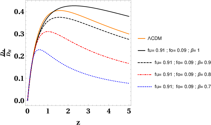
It can be seen from fig.1, that up to redshift around 1, almost all the curves are very close to that of the CDM case, while after a certain redshift, each of these curves start deviating from the CDM-curve. It can be ascertained that for a certain combination of and , this redshift-distance relation almost coincides with that of the CDM case. By numerical calculations using Mathematica, we find that for the combination and , with , variation of the quantity is almost identical to that of the CDM model.
As expected, departure from the CDM model increases for greater inhomogeneity, denoted by larger variation from the value of volume fractions . Next, in fig.2 we plot the ratio of angular diameter distance to the present Hubble length-scale w.r.t. redshift by varying the parameter for the combination of fractions and . We chose this value of combination as this is the combination, which has been indicated by N-body simulations of structure-formations for a two-partitioned Universe at present time Wiegand_et_al. It is seen that conformity with the homogeneous (CDM) model can be achieved for intermediate values of the void expansion parameter , whereas, the limiting cases of matter domination () and dark energy () lead to greater deviation from the CDM case.
The change in the observed redshift of a comoving source in the time interval of its observation is known as the redshift-drift. It can be given by , where is the time-rate of change of redshift and the suffix indicates its value at the observation time which has been taken as the present time . As the time scale of observation is generally much lesser than the time scale of cosmological evolution, the expression of the redshift-drift can be further simplified by applying the Taylor-series expansion, followed by neglecting the higher-order terms, as given below Koksbang:
| (19) |
where is the Hubble-parameter at the time of observation, which has been taken as the present time and is the Hubble-parameter at the time of emission of the signal.

The redshift-drift has been discussed in several works Koksbang; koksnew1; koksnew2; Koksbang-2; heinesen2. The analysis appears to be the same for the electromagnetic wave and gravitational wave sources, and the redshift-drift is directly proportional to the observation-time . However, the redshift drift is minimal for gravitational wave sources; specifically, the binaries of compact objects, viz., black holes and neutron stars, which have been observed by aLIGO or VIRGO ( is of the order of fractions of seconds to few minutes). Hence, the magnitude of the redshift-drift would be of very low order in these cases. However, for binaries of supermassive black holes, from which the gravitational wave signal is expected to be detectable by the future gravitational wave detectors like LISA, the time of observation can be of much higher order and hence, the redshift-drift’s magnitude should increase significantly for these type of binaries, especially at higher redshifts.
The sign of the redshift-drift indicates whether the Universe is accelerating or decelerating in the time interval of emission and observation of the signal, while its magnitude indicates the extent of the acceleration or deceleration. The expression of redshift-drift given in the equation (19) implies that for an accelerating Universe between the emission and observation times, the redshift-drift is positive. For a decelerating Universe between those times, it is negative. For the CDM model, we get the acceleration from a certain time in the late Universe, from which starts dominating over the matter till the present. So, for the CDM model, we can get a positive redshift-drift only after a certain redshift. For an inhomogeneous Universe described by Buchert’s backreaction formalism, the drift of the averaged redshift can be effectively described by replacing the Hubble-parameters’ values with the averaged Hubble-parameters Koksbang. However, as pointed out in Ref. Koksbang, the exact calculation of redshift-drift is obtained through a more elaborate process, and the drift of the averaged redshift may not represent the exact redshift-drift correctly.
The main motivation of our present analysis is to study the effect of inhomogeneities on parameters of gravitational wave sources, as discussed in detail in the next section. For the present, we will provide a calculation of the drift of averaged redshift. This is to reemphasize the role of inhomogeneities on the propagation of various signals (electromagnetic and gravitational) in the Universe, as computed through the backreaction formalism. In fig.3, we plot the drift of averaged redshift with respect to the redshift for the CDM model and our model with different combinations of the volume fractions and . By numerical calculations using Mathematica, we find that for the combination and , with , variation of the drift of averaged redshift is almost identical to that of the CDM model. 22 2 We choose a time-interval of observation 30 seconds, as for the typical binaries of compact objects, from which gravitational wave signals are detectable by aLIGO and VIRGO, the signal is observed within a time-duration of the order of fractions of seconds to minutes at most.
It may be noted from fig.3 that the drifts of averaged redshift are positive only up to a certain redshift for all the curves. The redshift at which the value of the drift of averaged redshift transits from positive to negative is different for each curve. This redshift of transition gradually decreases with an increase in or decrease in .
IV Change in gravitational wave observables in the backreaction framework
The gravitational wave amplitude from a binary of compact objects of masses and , in early inspiral stage where Keplerian approximations are well valid, is given by (for cross()-polarization) maggiore
| (20) |
where is the observed angular frequency of the binary of compact objects and is the luminosity-distance of the binary from the observer. For the plus()-polarization, the peak of the amplitude remains identical. The amplitude of the gravitational wave at the detector depends on the redshift at which it was generated. For a constant observed frequency, the redshift-dependent part in the gravitational wave amplitude is . It can also be expressed as , since , where is the cosmological-radial distance of the source. We study the variation of the quantity for the two cases: (i) a homogeneous and isotropic spacetime described by a flat FLRW metric in the CDM model, and (ii) an inhomogeneous region described by the backreaction formalism, keeping in view that in these two cases the variations of redshift are different.
To depict the change of variation of this quantity in the CDM model of the Universe and in the inhomogeneous Universe described by our two-partitioned model based on the Buchert’s backreaction formalism, we plot it w.r.t. redshift , in fig.4 for these two cases 33 3 We have kept the upper-limit of the redshift as 5, as accepted theories of cosmology predict the beginning of the structure-formation at the redshift 6 and without a proper structure formation this backreaction formalism can not be applied to model the Universe. For the CDM model, we have taken the values of and , with negligible , as is supported by most of the cosmological observations. .
For the inhomogeneous Universe, we use a set of different values of the fractions and , as was defined earlier for our two-partitioned model.


We see from fig.4 that as the source-redshift is increased, the deviation in the increases among different cases considered here. By numerical calculations using Mathematica, we find that for the combination and , with , variation of the quantity is almost identical to that of the CDM model. The deviation of this term for our two-partitioned model compared to that of the CDM-model increases immensely as we vary the values of and from the previously mentioned value. We also note that the values of the model parameters, at which the variation of the redshift dependent part of the gravitational wave amplitude with respect to redshift in our model becomes almost identical to the CDM-case, are different from the case for the drift of averaged redshift.
Now, we study the variation of w.r.t. for different values of the parameter , for the combination of fractions and . We see from the fig.5 that as the source-redshift is increased, the deviation in the term increases for different curves shown in this graph. Again, as is gradually decreased from the value 1, the deviation in the term increases for different curves. Using Mathematica, we find that for the value of the parameter , with the combination and , the variation of the quantity in our model is almost identical to that of the CDM model.
Therefore, it is evident that the observed gravitational wave amplitude is subject to change in our model, in comparison to that of the CDM model, while the amount of change depends on the effect of inhomogeneities in the domain consisting of the path of propagation of the gravitational wave signified by the model parameters , , and .
An interesting consequence of the changing variation of the redshift-dependent part of gravitational wave amplitude for our model in comparison with the CDM-model follows from noting the fact Rosado_et_al that the quantity has a minimum at given by
| (21) |
We note from the figs.4 and 5, that the quantity has different minima from that of the CDM-model with variation of the model parameters , and . It has been argued in Ref. Rosado_et_al that the equation (21) is independent of the gravitational wave detector, the model of cosmology under consideration, as well as the binary’s characteristics, provided its rest-frame frequency is in the inspiral phase. However, our study clearly indicates that although the equation (21) remains the same, the solution it gives for varies in case of our backreaction model. For the CDM-model the value of this minimum is . We note from fig.4 that decreases gradually with the increase in or decrease in for fixed . Besides this shifting of the , the minimum values of the quantity increases with increase in or decrease in . Again, we note from fig.5 that for the fixed combination and , decreases and the minimum value of the quantity increases if we decrease the parameter . This shifting can be said to be an effect of the local inhomogeneities that have been considered in our model.
V Conclusions
In this work, we have studied the propagation of gravitational waves from compact binary sources through a background spacetime which due to the presence of structures in the late time Universe, may not be correctly described by the flat FLRW metric at the relevant scales. In order to take into account the effect of inhomogeneities we have employed the Buchert’s backreaction formalism Buchert-1; Buchert-2; Wiegand_et_al in the framework of which we consider a two-partitioned toy model. Evolution under this model is shown to lead to a modification in the redshift versus distance relation as well as in the drift of the averaged redshift in comparison with the CDM model, in agreement with similar earlier results Koksbangwithin the backreaction framework.
Our analysis exhibits a substantial deviation in the variation of the redshift dependent part of the amplitude of gravitational waves generated from binaries of compact objects in their early inspiral stages, in the two cases, viz., (i) the CDM model, and (ii) our model based on Buchert’s backreaction formalism. We have investigated the latter model for various combinations of the model parameters such as the volume fractions of overdense and underdense regions, as well as the rate of expansion of the underdense region. We find that only for very specific combinations of the above parameters, the variation of the redshift dependent part of the amplitude of gravitational wave matches with that of the CDM case. The deviation of the variation increases with the increasing effect of inhomogeneities quantified by the volume fractions and the void expansion rate. Our results further display an interesting shift in the minima of the redshift dependent part of the gravitational wave amplitude, which is a clear consequence of the backreaction from inhomogeneities.
Before concluding, we would like to make the following comments. In the present era of precision cosmology with several upcoming probes, the determination of properties of distant sources of gravitational waves will play an important role in several domains of astrophysics and cosmology. The significance of precise determination of gravitational wave observables have spurred many recent works on ascertaining the role of effects such as primordial black hole accretion bellido; arnab, and various phase transitions and inflationary scenarios guo. On the other hand, our present work investigates the role of observed structure Sloan; WiggleZDE in the Universe on gravitational wave propagation, using the backreaction framework Buchert-1; Buchert-2; Wiegand_et_al without invoking non-standard physics. Through our analysis we have found a clear signature of backreaction in the shift of the gravitational wave amplitude minima in the context of our simplified two-domain model. Our present analysis should inspire further detailed calculations using more sophisticated backreaction scenarios, such as multi domain models, in order to provide more accurate predictions of the quantitative deviation of gravitational wave observables from those obtained in CDM cosmology.
Acknowledgements: The authors thank Sophie Marie Koksbang for an important comment related to our work. The authors would also like to thank the anonymous referee whose comments have led to significant improvements in the presentation. SSP thanks the Council of Scientific and Industrial Research (CSIR), Govt. of India, for funding through CSIR-JRF-NET fellowship. AS thanks S. N. Bose National Centre for Basic Sciences, Salt lake city, Kolkata-700106, under Department of Science and Technology (DST), Govt. of India, for funding through institute-fellowship.
References
- (1) A. Einstein, Näherungsweise Integration der Feldgleichungen der Gravitation, Sitzungsberichte der Königlich Preußischen Akademie der Wissenschaften (Berlin) (1916) Seite 688-696,.
- (2) A. Einstein, Über Gravitationswellen , Sitzungsberichte der Königlich Preuischen Akademie der Wissenschaften (Berlin) (1918) Seite 154-167.
- (3) B. P. Abbott et al., Observation of Gravitational Waves from a Binary Black Hole Merger, Phys. Rev. Lett. 116 (2016) 061102.
- (4) LIGO-VIRGO Collaboration, GW151226: Observation of Gravitational Waves from a 22-Solar-Mass Binary Black Hole Coalescence, Phys. Rev. Lett. 116 (2016) 241103.
- (5) LIGO-VIRGO Collaboration, GW170104: Observation of a 50-Solar-Mass Binary Black Hole Coalescence at Redshift 0.2, Phys. Rev. Lett. 118 (2017) 221101.
- (6) LIGO-VIRGO Collaboration, GW170814: A Three-Detector Observation of Gravitational Waves from a Binary Black Hole Coalescence, Phys. Rev. Lett. 119 (2017) 141101.
- (7) LIGO-VIRGO Collaboration, GW170817: Observation of Gravitational Waves from a Binary Neutron Star Inspiral, Phys. Rev. Lett. 119 (2017) 161101.
- (8) LIGO-VIRGO Collaboration, GW170608: Observation of a 19 Solar-mass Binary Black Hole Coalescence, Astrophys. J. 851 (2017) L35.
- (9) D. W. Hogg et al., Cosmic homogeneity demonstrated with luminous red galaxies, Astrophys. J. 624 (2005) 54 [arXiv:astro-ph/0411197].
- (10) M. Scrimgeour et al., The WiggleZ Dark Energy Survey: the transition to large-scale cosmic homogeneity, Mon. Not. Roy. Astron. Soc. 425 (2012) 116 arXiv:1205.6812v2 [astro-ph.CO]
- (11) A. Wiegand, T. Buchert and M. Ostermann, Direct Minkowski Functional analysis of large redshift surveys: a new high-speed code tested on the luminous red galaxy Sloan Digital Sky Survey-DR7 catalogue, Mon. Not. Roy. Astron. Soc. 443 (2014) 241-259, https://doi.org/10.1093/mnras/stu1118 arXiv:1311.3661v2 [astro-ph.CO].
- (12) M. F. Shirokov and I. Z. Fisher, Isotropic space with discrete gravitational field sources. on the theory of non homogeneous isotropic universe, Sov. Astron. J. 6 (1963) 699 Reprinted in: Gen. Rel. Grav. 30 (1998) 1411.
- (13) G. F. R. Ellis, Relativistic cosmology: its nature, aims and problems, Gen. Rel. Grav., Eds. B. Bertotti et al. (Reidel, Dordrecht) (1984) pp. 215.
- (14) T. Futamase, Approximation scheme for constructing a clumpy universe in General Relativity, Phys. Rev. Lett. 61 (1988) 2175.
- (15) T. Futamase and M. Sasaki, Light propagation and the distance-redshift relation in a realistic inhomogeneous universe, Phys. Rev. D 40 (1989) 2502.
- (16) R.M. Zalaletdinov, Averaging out the Einstein equations, Gen. Rel. Grav. 24 (1992) 1015.
- (17) R.M. Zalaletdinov, Towards a theory of macroscopic gravity, Gen. Rel. Grav. 25 (1993) 673.
- (18) T. Buchert, On average properties of inhomogeneous fluids in general relativity I: dust cosmologies, Gen. Rel. Grav. 32 (2000) 105 [arXiv:gr-qc/9906015].
- (19) T. Buchert, On average properties of inhomogeneous fluids in general relativity II: perfect fluid cosmologies, Gen. Rel. Grav. 33 (2001) 1381 [arXiv:gr-qc/0102049].
- (20) D. J. Schwarz, Accelerated expansion without dark energy, In: On the nature of dark energy, 18th IAP Astrophysics Colloquium, Eds. P. Brax et al. (2002) pp. 331 [arXiv:astro-ph/0209584].
- (21) S. Räsänen, Dark energy from backreaction, JCAP 0402 (2004) 003 [arXiv:astro-ph/0311257].
- (22) D. L. Wiltshire, Dark energy without dark energy, In: Dark Matter in Astroparticle and Particle Physics, Eds. H.V. Klapdor-Kleingrothaus and G.F. Lewis (2008) pp. 565 [arXiv:0712.3984].
- (23) E.W. Kolb et al. , On cosmic acceleration without dark energy, New J. Phys. 8 (2006) 322 [arXiv:astro-ph/0506534].
- (24) A. Ishibashi and R. M. Wald, Can the Acceleration of Our Universe Be Explained by the Effects of Inhomogeneities ? Class. Quant. Grav. 23 (2006) 235 [arXiv:gr-qc/0509108].
- (25) A.A. Coley, Null geodesics and observational cosmology (2008) [arXiv:0812.4565].
- (26) S. Räsänen, Evaluating backreaction with the peak model of structure formation, JCAP 0804 (2008) 026 [arXiv:0801.2692].
- (27) S. Räsänen, Light propagation in statistically homogeneous and isotropic dust universes, JCAP 0902 (2009) 011 [arXiv:0812.2872].
- (28) M. Gasperini et al., Gauge invariant averages for the cosmological backreaction, JCAP 0903 (2009) 011 [arXiv:0901.1303].
- (29) M. Gasperini et al., Light-cone averaging in cosmology: formalism and applications, JCAP 1107 (2011) 008 [arXiv:1104.1167].
- (30) N. Bose and A. S. Majumdar, Future deceleration due to cosmic backreaction in presence of the event horizon, Mon. Not. Roy. Astron. Soc. : Letters 418 Issue 1 (2011) L45–L48 https://doi.org/10.1111/j.1745-3933.2011.01140.x
- (31) P. Fleury et al., Interpretation of the Hubble diagram in a nonhomogeneous universe Phys. Rev. D 87 (2013) 123526 [arXiv:1302.5308].
- (32) N. Bose and A. S. Majumdar, Effect of cosmic backreaction on the future evolution of an accelerating universe, Gen. Relativ. Gravit. 45 (2013) 1971-1987 arXiv:1203.0125 [astro-ph.CO].
- (33) P. Fleury et al., Can all cosmological observations be accurately interpreted with a unique geometry? Phys. Rev. Lett. 111 (2013) 091302 [arXiv:1304.7791].
- (34) P. Fleury, Swiss-cheese models and the Dyer-Roeder approximation (2014) [arXiv:1402.3123]
- (35) S. Bagheri and D. J. Schwarz, Light propagation in the averaged universe, JCAP 10 (2014) 073 arXiv:1404.2185 [astro-ph.CO].
- (36) A. Ali and A. S. Majumdar, Future evolution in a backreaction model and the analogous scalar field cosmology, JCAP 01 (2017) 054 arXiv:1608.01608 [gr-qc].
- (37) S. M. Koksbang, Another look at redshift drift and the backreaction conjecture, JCAP 10 (2019) 036 arXiv:1909.13489 [astro-ph.CO].
- (38) A. Wiegand and T. Buchert, Multi-scale cosmology and structure-emerging Dark Energy: a plausibility analysis, Phys. Rev. D 82 (2010) 023523 [arXiv:1002.3912].
- (39) S. M. Koksbang, Observations in statistically homogeneous, locally inhomogeneous cosmological toy models without FLRW backgrounds, Mon. Not. Roy. Astron. Soc. : Letters, 498, Issue 1, (2020), L135-L139, https://doi.org/10.1093/mnrasl/slaa146 arXiv:2008.07108 [astro-ph.CO]
- (40) A. Heinesen, Multipole decomposition of the general luminosity distance Hubble law — a new framework for observational cosmology, JCAP 05 (2021) 008 arXiv:2010.06534 [astro-ph.CO].
- (41) S. M. Koksbang, Searching for Signals of Inhomogeneity Using Multiple Probes of the Cosmic Expansion Rate , Phys. Rev. Lett. 126 (2021) 231101 arXiv:2105.11880v1 [astro-ph.CO]
- (42) A. H. Nitz et al, 1-OGC: The First Open Gravitational-wave Catalog of Binary Mergers from Analysis of Public Advanced LIGO Data, Astrophys. J. 872 195 (2019).
- (43) B. P. Abbott et al, (LIGO Scientific Collaboration and Virgo Collaboration), GWTC-1: A Gravitational-Wave Transient Catalog of Compact Binary Mergers Observed by LIGO and Virgo during the First and Second Observing Runs, Phy. Rev. X 9, 031040 (2019).
- (44) A. N. Baushev, The central region of a void: an analytical solution, Mon. Not. Roy. Astron. Soc. :Letters 504, Issue 1 (2021) L56-L60 arXiv:2104.01359 [astro-ph.CO].
- (45) S. M. Koksbang and S. Hannestad, Redshift drift in an inhomogeneous universe: averaging and the backreaction conjecture, JCAP 01 (2016) 009 arXiv:1512.05624v2 [astro-ph.CO].
- (46) J. Larena et al., Testing backreaction effects with observations, Phys.Rev. D 79 (2009) 083011 arXiv:0808.1161v2 [astro-ph]
- (47) E. Rosenthal and E. E. Flanagan, Cosmological backreaction and spatially averaged spatial curvature, arXiv:0809.2107v1 [gr-qc]
- (48) A. Paranjape and T. P. Singh, Explicit Cosmological Coarse Graining via Spatial Averaging, Gen.Rel.Grav. 40 (2008) 139-157 arXiv:astro-ph/0609481v4.
- (49) S. Räsänen, Light propagation in statistically homogeneous and isotropic universes with general matter content, JCAP 1003 (2010) 018 arXiv:0912.3370v2 [astro-ph.CO]
- (50) S. M. Koksbang, Towards statistically homogeneous and isotropic perfect fluid universes with cosmic backreaction, Class. Quantum Grav. 36 (2019) 185004 arXiv:1907.08681v1 [gr-qc].
- (51) A. Heinesen, Multipole decomposition of redshift drift: Model-independent mapping of the expansion history of the Universe, Phys. Rev. D 103 023537 (2021) arXiv:2011.10048v1 [gr-qc].
- (52) M. Maggiore, Gravitational waves: theory and experiments, (Oxford University Press, New York, 2008).
- (53) P. A. Rosado, P. D. Lasky, E. Thrane, X. Zhu, Ilya Mandel, and A. Sesana, Detectability of Gravitational Waves from High-Redshift Binaries , Phy. Rev. Lett. 116 (2016) 101102 arXiv:1512.04950v2 [astro-ph.CO]
- (54) J. Garcia-Bellido, Massive Primordial Black Holes as Dark Matter and their detection with Gravitational Waves, J. Phys.: Conference Series 840, 012032 (2017).
- (55) A. Sarkar, K. R. Nayak and A. S. Majumdar, Stochastic gravitational wave background from accreting primordial black hole binaries during early inspiral stage, Phys. Rev. D 100 (2019) 103514 arXiv:1904.13261v2 [astro-ph.CO].
- (56) H.-K. Guo, K. Sinha, V. Daniel and G. White, Phase transitions in an expanding universe: stochastic gravitational waves in standard and non-standard histories, JCAP 01 (2021) 001 arXiv:2007.08537v3 [hep-ph].