Baryogenesis from combined
Higgs – scalar field inflation
Yann Cado,
Mariano Quirós
Institut de Física d’Altes Energies (IFAE) and
The Barcelona Institute of Science and Technology (BIST),
Campus UAB, 08193 Bellaterra, Barcelona, Spain
Abstract
We study a modification of the Higgs inflation scenario where we introduce an extra scalar , with mass , coupled to the Ricci scalar as , and mixed with the Higgs field via the Lagrangian term . Both fields participate in the inflation process in a unitary theory that predicts values of the cosmological observables in agreement with the results from the Planck/BICEP/Keck collaborations. In addition, by means of a -odd effective operator that couples to the Chern-Simons term of the hypercharge gauge group as , maximally helical magnetic fields are produced during the last -folds of inflation. We found a window in the coupling where these fields survive all constraints until the electroweak phase transition, and source the baryon asymmetry of the Universe through the Standard Model chiral anomaly. From a phenomenological perspective, the model can solve the Standard Model instability problem at the scale GeV, provided that , and for (few) TeV, the - mixing becomes sizable while the theory turns natural. The latter thus predicts modifications of the trilinear and quartic couplings that could be explored at the HE-LHC, as well as at future colliders, and allows for direct production at the LHC followed by decay into . Present results from ATLAS and CMS already put (mild) bounds on the mass of the heavy scalar as TeV at 95% C.L.
1 Introduction
Electroweak (EW) baryogenesis is an appealing mechanism to understand the baryon asymmetry of the Universe (BAU) Sakharov:1967dj (for reviews see Refs. Cohen:1993nk; Quiros:1994dr; Rubakov:1996vz; Carena:1997ys; Quiros:1999jp; Morrissey:2012db), which is testable at EW energies. Although the Standard Model (SM) contains all necessary ingredients required by the three Sakharov conditions, it quantitatively fails as the amount of -violation in the CKM phase is too small and moreover, given the experimental value of the Higgs mass, the electroweak phase transition (EWPT) is not strong enough first order, but a continuous crossover DOnofrio:2015gop; Kajantie:1996qd. This mechanism should then require beyond the SM physics.
It was more recently realized, Refs. Anber:2006xt; Bamba:2006km; Bamba:2007hf; Anber:2009ua; Anber:2015yca; Cado:2016kdp; Sfakianakis:2018lzf, that maximally helical hypermagnetic fields can be produced at the end of (axial) inflation, and can generate the observed BAU, via the anomaly, during the EWPT. In this kind of theories, is spontaneously violated by the effective dimension-five operator , where is the axial field, the strength of the hypercharge gauge field , and its dual, whose generation requires an ultraviolet (UV) completion of the model. The generation of the observed BAU was further elaborated in a number of papers, see e.g. Refs. Kamada:2016eeb; Kamada:2016cnb; Jimenez:2017cdr; Domcke:2019mnd.
In a recent paper Cado:2021bia, we proposed a mechanism where the helical hypermagnetic fields were produced after inflation by the Higgs doublet field with a -violating dimension-six operator, thus entirely relying the nonperturbative production of gauge fields on SM physics. Of course generating the -odd operator requires a UV completion, which can be similar to that giving rise to the -even operator , for which is (spontaneously) violated for background values of the axial field .
Moreover there are theories, dubbed as Higgs inflation (HI) models Bezrukov:2007ep; Bezrukov:2008ej; Bezrukov:2010jz (for a review see Rubio:2018ogq), where the inflaton is identified with the SM Higgs boson, thus linking the cosmological observables during the inflationary period of inflation with SM quantities. These models are based on assuming, in the Jordan frame, a coupling between the Higgs doublet and the Ricci scalar as , where the ellipses refers to the SM Lagrangian. This model has been shown to have a (dynamical) cutoff , for values of the Higgs at the electroweak scale, i.e. Han:2004wt; Burgess:2009ea; Barbon:2009ya; Lerner:2009na; Burgess:2010zq; Hertzberg:2010dc, while at values of the Higgs where inflation happens, i.e. , the cutoff has been proven to be , at least for two-by-two tree level scattering amplitudes, avoiding thus unitarity violation Antoniadis:2021axu; Ito:2021ssc; Karananas:2022byw. Moreover, HI models have to face another challenge: for actual values of the Higgs boson and top-quark masses the SM potential becomes unstable at values of the Higgs field GeV. This question has been tackled in Ref. Bezrukov:2014ipa, where the case of an unstable potential was considered, taking into account radiative corrections. Because of the Higgs-Ricci coupling the theory becomes nonrenormalizable in the Einstein frame and requires the addition of an infinite number of counterterms. By assuming a scale invariant UV completion it is found that there are threshold effects at scales which generate jumps of the SM quartic coupling to positive values (although one cannot determine their amplitude from the theory) and therefore HI can proceed in the usual way. Still the potential has two minima: the EW minimum and a much deeper (unphysical) minimum associated to the instability of the original SM potential. The evolution of the Higgs field after inflation will depend on the reheating process, and in particular on the reheating temperature. If the reheating temperature is high enough such that the unphysical minimum is dominated by the thermal corrections, then the Higgs will relax to the symmetric phase, otherwise the Higgs would go to the unphysical vacuum and it would stay there forever.
Motivated by HI, we will propose a model where the SM potential is simply stabilized by a scalar field coupled to the Higgs (this coupling was already pursued in Refs. Giudice:2010ka; Barbon:2015fla) and with a mass , opening up the possibility of direct or indirect detection at present (LHC) and future accelerators. Moreover if the stabilizing field has a weak enough self-coupling and is coupled to the Ricci tensor as , it can trigger cosmological inflation, as the potential becomes flat in the Einstein frame, while the COBE normalization does not impose strong constraints on the coupling. In this theory the inflaton can couple to the Chern-Simons component of the SM hypercharge and trigger baryogenesis via the production of helical magnetic fields. Finally through the coupling of the inflaton and the Higgs field, the latter will also be a component of the inflaton sector, although we will work out a model where the parameters are such that cosmological inflation will be mainly driven by the stabilizing field . The model thus combine HI, baryogenesis via production of helical magnetic fields and stabilization of the SM potential by modifying the renormalization group running, to provide a successful history of the Universe.
In the present paper we will follow the above guideline in order to build such a model of inflation, which consists in a modification of the HI model by the introduction of a scalar field , with a two-field potential in which analytical relations between both fields are enforced by its shape. One major difference with respect to a previous attempt, Ref. Barbon:2015fla, is that is coupled to the Ricci scalar as , with 11 1 It has been proved, in Refs. Hertzberg:2010dc; Lerner:2009na, that there is no tree-level unitarity problem for the amplitude as, in the Einstein frame, see Eq. (2.30), there appears the effective operator that—upon integration by parts gives, on-shell, the correction —leads to a four-point function that does not grow with the energy, and thus does not violate unitarity. A similar result is obtained in the Jordan frame, where the amplitude grows, in the -channel, with the energy, and behaves as . However, considering the cross channels, there is a cancellation, and the four-point amplitude behaves as . However, the quick conclusion that unitarity is not violated at the scale has been challenged in Refs. Hertzberg:2010dc; Burgess:2010zq, where it was pointed out that, in the Jordan frame, the above cancellation is very unlikely to appear in loop-induced corrections to the same process , leading to a cutoff at the value , where a loop factor has been included. The observation is similar for higher order processes, since e.g. has a cross section that scales as , where is the quartic coupling. This indicates that the perturbative description breaks down for energies , which goes to for large values of . Similarly, in the Einstein frame, on top of the nonproblematic effective operator , other higher order operators, as e.g. , are expected to be generated by loop effects, and so are expected to trigger violations of unitarity beyond the scale . In view of these arguments we will conservatively consider in this paper as the scale at which unitarity is violated., where is the theory cutoff, while , thus satisfying the most naive unitarity requirement. Therefore, in our model the Higgs field is not the only inflaton, but a component of the inflaton system, as inflation is really driven along a particular path in the two-field space, while its orthogonal direction has a strong curvature around its minimum, where the field system is anchored.
This paper is organized as follows. In Sec. 2 we introduce the potential in the Jordan frame, as a function of the fields and , which (for Planckian values of the field ) can be approximated by the most general renormalizable polynomial satisfying the symmetry . As the Ricci term is quadratic in , , the beginning of inflation will be controlled by the quartic term , and the size of the amplitude of density perturbations is provided by the smallness of , for values of , consistent with the naive unitarity of the theory. The smallness of the coupling is stable under radiative corrections, and so is technically natural, but the Higgs potential is unstable for values of the renormalization scale GeV. If the mass of the field is , the field decouples for values of . Then, in the presence of a potential term softly breaking the symmetry, , there is a threshold correction in the one-loop function of the Higgs quartic coupling that can stabilize the EW vacuum. This mechanism was introduced in Ref. Barbon:2015fla and we will use it to constrain our parameter space.22 2 Should we have, instead, considered a linear Ricci term, , and a quadratic, , inflationary potential, one could also have achieved the amount of flatness required by the slow roll conditions during the inflationary period, but the size of the amplitude of density perturbations, now controlled by , would have yielded a value , which is too large to stabilize the EW vacuum.
The properties of the inflationary model are presented in Sec. 3. There, we will prove that all observational constraints from the Planck and BICEP/Keck collaborations on the slow roll parameters, or equivalently on the spectral index, the spectral index running and the tensor-to-scalar ratio, can be satisfied for a range of the parameter such that , thus easily satisfying the unitarity condition for the model.
The nonperturbative production of gauge fields at the end of inflation is presented in Sec. 4. In particular we will consider the -violating dimension-five operator , provided by some UV completion, to trigger baryogenesis at the EWPT. We postpone to App. A the details of a particularly simple UV completion giving rise to such an operator. Similar UV completions were proposed in Ref. Dine:1990fj, and recently in Refs. Carena:2018cjh; Carena:2019xrr, to generate the BAU using various mechanisms, so we can be agnostic about its origin. We have found a critical value of the parameter , such that for the backreaction of the produced gauge fields on the inflationary dynamics can be neglected, and so we have explicitly considered this region in the numerical analysis. Moreover, in the presence of magnetic fields, as those produced in this work, there appear fermionic currents, a phenomenon called the Schwinger effect, and, for sufficiently strong magnetic fields, their backreaction on the gauge fields cannot be neglected. As exactly solving the equations of motion of gauge fields, in the presence of the Schwinger fermionic currents, is beyond the scope of the present paper, we have followed recent proposals in the literature for gauge field estimates Domcke:2018eki; Domcke:2019mnd, and have worked out two simple approximations: the maximal estimate, obtained upon maximizing the value of the helicity, and the equilibrium estimate. A detailed recent analysis Gorbar:2021zlr shows that the exact solutions lie in between both estimates, so we can reliably corner the final allowed region in the relevant parameter space.
The reheating mechanism has been studied in Sec. 5, and we have consistently considered the region , where the reheating takes place perturbatively by the leaading inflaton decay process . The inflaton width, as well as the reheating temperature , are then functions of the inflaton mass parameter . In order to stabilize the EW vacuum, the latter must lie in the interval which implies, for reheating temperatures, the interval , where GeV would be the instant reheating temperature, i.e. the reheating temperature in the hypothetical case where equals the Hubble parameter at the end of inflation.
We show in Sec. 6 how the baryon asymmetry is generated when helicity transforms into baryon number at the EW crossover. In particular we show that this mechanism works for , and provides an upper bound on which depends on the value of the reheating temperature.
In Sec. 7 we consider all relevant conditions for the helical magnetic fields to survive from the end of inflation, when they are generated, to the EWPT, when they convert into the baryon asymmetry. In particular we have considered the constraints from magnetohydrodynamics (MHD) and Reynolds numbers, from chiral plasma instability, from the non-Gaussianity of the inflaton primordial fluctuations and from the baryon isocurvature perturbations. Some technical details about the latter are postponed to App. B. Globally they constrain the region where the baryogenesis mechanism works, leaving an allowed range for the values of the parameter , which depends on the ratio . Readers not interested in the technical details of the analysis can straightforwardly go to Sec. 7.5, and in particular to Fig. 9, which summarizes the combined results.
In Sec. 8 some phenomenological considerations, from the point of view of particle physics, are presented. First of all we study the naturalness problem generated by the mass hierarchy , where is the Higgs mass, which leads either to a fine-tuning or considering (TeV). The latter case is phenomenologically appealing as the -breaking term in the potential generates a mixing between the singlet and the Higgs field . This mixing, which is negligible in the case of very large values of the parameter , can be sizable, and with relevant phenomenological applications, for the case of (TeV) and, furthermore, is already bounded by the present LHC measurements of Higgs signal strengths. As the mixing angle is inversely proportional to , the latter already provide mild lower bounds on , as TeV, a region where electroweak observables are shown to be in agreement with their experimental values. Moreover, the mixing introduces modifications on the SM parameters and , which could lead to constraints at the HE-LHC at TeV, or even in future colliders with center of mass energies of 100 TeV. Finally the singlet state can be produced at LHC by means of its mixing with the Higgs field. Present upper bounds, from the ATLAS and CMS collaborations, on the production cross section lead to upper bounds on the mixing parameter and, consequently, to lower bounds on as TeV at 95% C.L., while future runs are expected to provide stronger bounds on it.
Finally we summarize the results and present our conclusions in Sec. 9.
2 The model
As stated in the previous section we consider, on top of the Higgs field , the scalar field with the Lagrangian as 33 3 In our notation the Lagrangian will not contain the factor , so that the action is given by .
| (2.1) |
which contains a coupling of the field to the Ricci scalar 44 4 Notice that in our model we do not need to primarily introduce any term. Although a small value of the parameter will be generated anyway by radiative corrections Espinosa:2015qea, its effects on the inflation mechanism will always be negligible, even for values of ; so for simplicity we are assuming that ., and the potential is given by
| (2.2) | ||||
The first four terms of the potential in Eq. (2.2) constitute the most general renormalizable potential invariant under the symmetry, , while the last term is a soft breaking of such symmetry. Besides, for large Higgs field configurations we will be neglecting the mass term , as compared to the term, in .
The parameters and should be constrained by the slow roll conditions during inflation to very small values , as we will see later on. Their smallness is radiatively stable, as can easily be deduced from their one-loop functions 55 5 We are defining conventionally here .
| (2.3a) | |||||
| (2.3b) | |||||
where , and is the renormalization scale. In particular the choice is technically natural at one loop, as can be seen from Eq. (2.3a). For simplicity we will adopt hereafter the value . Moreover, from the amplitude of density perturbations, we will see that typically , a value that is very mildly changed by radiative corrections.
2.1 Jordan frame
The previous Lagrangian is defined in the so-called Jordan frame, and it is a valid framework provided that the field satisfies the condition . This region, as we will see, encompasses part of the inflationary period, and in particular the end of inflation. The trajectory of fields and will proceed along the submanifold given by the minimum of the two-dimensional potential surface, providing a relationship between both fields, as anticipated in the introduction of this paper.
To find the relationship between both fields and , along the potential minimum direction, we will follow a general procedure summarized here. Given a potential of two fields and , the contour lines corresponding to constant values of the function , satisfy the relation , which reads
| (2.4) |
where, by definition, the function is the slope along the contour lines at the point . We wish to find the direction that intersects orthogonally every contour line. The slope of this line is obviously and the slope of the orthogonal line is , so the condition for the orthogonal intersection is
| (2.5) |
The idea behind the regions is to divide the potential valley into segments such that . The regions are separated according to which term dominates in the potential. Hence, we will find it useful to work with logarithmic variables
| (2.6) |
where the and fields are considered in some arbitrary mass units, such that the relation between fields translate into straight lines . Given the shape of our potential we find a unique solution to (2.5) in each region.
The direction that intersects orthogonally every contour line in the plane is given by the solution to the equation
| (2.7) |
Therefore, the trajectory in the plane is given by relation (2.7), which changes according to the different regions of the potential that we will now introduce. This is validated by the plot of the total potential exhibited in Fig. 1. In all cases, the valley acts as an attractor for the fields, as shown in Ref. Barbon:2015fla.
Region A
In this region both fields take their maximum allowed values in the Jordan Frame, and the potential can be approximated by the quartic coupling terms
| (2.8) |
The direction along the minimum can be found, after applying Eq. (2.7) to the potential (2.8), with the function , i.e.
| (2.9) |
We plot in Fig. 1 the complete inflationary potential in the Einstein frame (see Sec. 2.3) and show the direction from Eq. (2.9) with a solid (green) line as specified in the figure caption.


Its region of validity is then given by
| (2.10) |
where we have defined the constant as
| (2.11) |
Along the minimum direction (2.9) the potential can be written, as a function of , as
| (2.12) |
which will be used in the next section to describe the end of inflation.
To make contact with HI results, in this region we can also use the Higgs field as the explicit variable using the relation between the fields and given by Eq. (2.9). This implies that the Ricci term in Eq. (2.1) can be equivalently written as , with . For typical values of the parameters (e.g. , see Secs. 2.2 and 3), we get , which is the value required by HI. Moreover the potential (2.12) can be written, using again (2.9) as
| (2.13) |
This result shows how, in region A, the results of HI could be interpreted in our model with , being perfectly consistent with the unitarity condition .
Region B
In this region, where
| (2.14) |
the potential can be approximated by
| (2.15) |
which, using Eq. (2.7), has its minimum along the direction
| (2.16) |
Direction (2.16) is shown in the potential plot, Fig. 1, with a solid (magenta) line. If we define the coupling as
| (2.17) |
in the limit we can write the minimum condition as
| (2.18) |
and the potential (2.15) becomes
| (2.19) |
which shows that the effective quartic coupling in this region is given by , instead of as in the original potential (2.2).
Region C
In this region , where is the Higgs vacuum expectation value (VEV) and , the renormalization scale, is here identified with the classical value of the Higgs field . The field hence decouples and is integrated out as
| (2.20) |
which yields a potential
| (2.21) |
Notice that, to leading order, the solution to the equation of motion of , Eq. (2.20), agrees with the minimum condition in Region B, Eq. (2.18), which guarantees the continuity between both regions. Moreover the stability of the potential in both Regions B and C is provided by the same condition, .
2.2 Stability of the potential
In Region C, , the inflaton field is integrated out and the potential, as a function of the Higgs , is given by Eq. (2.21), so that the parameter runs as the quartic coupling in the SM potential, according to the SM function, . In Regions B and A, , the inflaton propagates and thus there is an extra contribution to the running of the parameter as Barbon:2015fla
| (2.22) |
where is the Heaviside function, equal to 1 (0) for (), and . The parameter also runs with the renormalization scale as
| (2.23) |
The extra contribution to the running of in Eq. (2.22) can solve the Higgs vacuum instability problem provided that:
- •
The inflaton mass is smaller than the SM instability scale, GeV.
- •
The value of at the scale , , is large enough in order to significantly change the value of .
Of course, smaller values of (i.e. wider regions where propagates) allow smaller values of to satisfy the second criterion. Conversely, for values of close to the minimum value of that solves the instability is a largish one.
As we have seen, the condition for the stability of the potential is that the coupling defined in Eq. (2.17) is positive definite, . We have solved at two-loop the RGE’s of the theory for the following set of values of the input parameters Khoury:2021zao at the pole top mass GeV,
| (2.24) | ||||
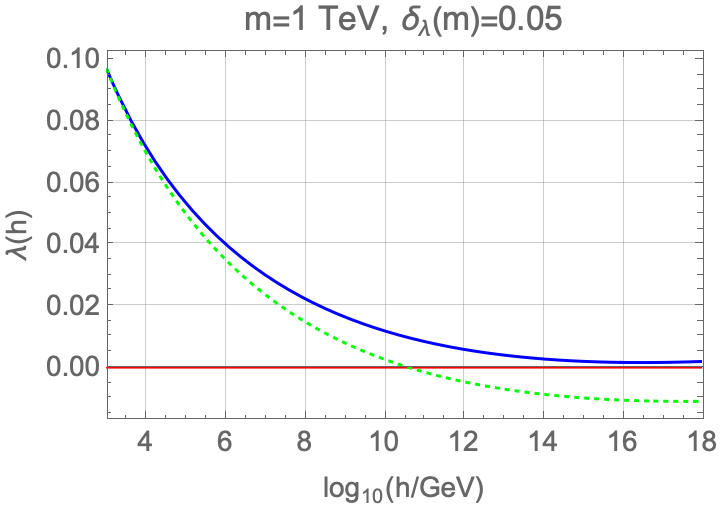

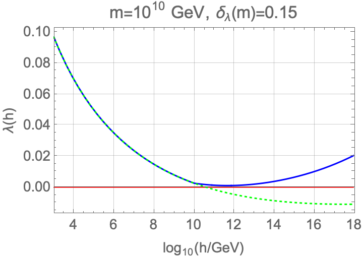
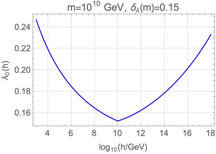
In Fig. 2 we show the two-loop running of the parameters and for two extreme cases, with a light ( TeV, upper panels) and a heavy ( GeV, lower panels) inflaton. As we can see typical values of are smaller for smaller values of . We have chosen for TeV, and for GeV. In both cases the value of can be tuned to smaller values, such that the corresponding values of at high scales are smaller. On the other hand, larger values of are bound by imposing that the theory remains in the perturbative regime up to the high scale. In particular we find, for large values of , , , while for in the TeV region, . The dashed lines in the left panels are the SM running, shown for comparison. On both left panels, we can see that the condition is satisfied while at .
2.3 Einstein frame
For values of the field such that we must redefine the metric and go to the so-called Einstein frame to recover the Einstein-Hilbert action for the Ricci scalar. To do so, we perform a Weyl redefinition of the metric:
| (2.25) |
For the Ricci scalar this implies
| (2.26) |
Note that is absent in the correction term , hence we will define by demanding that the explicit coupling between and disappears from the Lagrangian in the Einstein frame. The Ricci part of the action transforms then as
| (2.27) |
and so the definition
| (2.28) |
leads to
| (2.29) |
We can see from the second (dimension-six effective operator) term in Eq. (2.29) that the cutoff of the theory is identified as (see however comments in footnote 1).
In the meantime the kinetic terms of and get transformed to so that the (noncanonical) kinetic terms are given by
| (2.30) |
leading to the action in the Einstein frame
| (2.31) |
where the Einstein frame potential is given by
| (2.32) |
and is given by Eq. (2.2). The potential region where the values of the field satisfy the condition is denoted as Region and is explored hereafter.
Region
As just stated, the Region is characterized by the potential in the Einstein frame, i.e. Eq. (2.32) for , and a straightforward application of Eq. (2.5) shows that, using Eq. (2.7), the direction along the minimum in the two-dimensional potential is given by
| (2.33) |
from where the function in Eq. (2.7) can easily be read out. Along this direction the potential is
| (2.34) |
where again the last equality comes from the very definition of the region. Notice that the values of the field at the beginning of inflation, and in particular its value at horizon crossing of the present Universe, belong to Region .
In Fig. 1 we plot the potential in the Einstein frame for a chosen set of the parameters values, and we superimpose the lines of minimum submanifolds given by Eqs. (2.33), (2.10) and (2.16), for Regions , A and B, respectively. As we can see they intersect orthogonally, by construction, the contour lines of the potential. In the left panel we plot the contour lines of the potential and in the right panel the three-dimensional plot with the same color codes.
We can try to make contact with HI in Region , as we did in Region A, using the Higgs field as the explicit variable, by means of the relation between the fields and given in Eq. (2.33), which we can write as
| (2.35) |
The Ricci coupling can then be written as , where by using the typical values of the parameters, (see Secs. 2.2 and 3). Similarly, we can also write the potential as
| (2.36) |
These two expressions show that our model, written in terms of the Higgs field, departs from the conventional HI as it requires an effective dimension-eight operator for the potential which could only appear when the Standard Model is completed by some UV theory, giving rise, after decoupling, to higher dimensional operators.
3 Inflation
Inflation takes place only in Regions (for ), and A (for ), thus we will choose conditions (2.33) and (2.9), respectively, to relate and . In this case the kinetic term (2.30) along the minimum direction can be written in both Regions and A, as
| (3.1) |
where corresponds to the (tiny) contribution of the Higgs kinetic term
| (3.2) |
and the last inequality comes from the condition . Putting numbers we obtain that and , so that can be safely neglected for numerical calculations in Eq. (3.1).
As for the potential in both inflationary regions, and A, using the previous results we can write it as
| (3.3) |
so that, in both regions, they only differ by a global factor. As the slow roll parameters do depend on ratios of the potential and its derivatives, they will not depend on the global factor and can thus be given a universal expression. So for the computation of the slow roll parameters we will just remove the global factor and use as the inflationary potential.
We can now define the inflaton as a field with canonical kinetic term as
| (3.4) |
where the change of variable is done by
| (3.5) |
the last equality simply being the definition of the function for later use. Solving the above differential equation gives the approximation
| (3.6) |
which, for , can be inverted to get
| (3.7) |
while , for , as in this limit the Jordan and Einstein frames should coincide.
However, although the slow roll parameters must be computed from the inflaton potential , we will not need to use this explicit solution to obtain the inflationary parameters. Instead, we can keep as the explicit variable, since performing the change of variables (3.5) in the slow roll parameters definition allows us to avoid making inevitable approximations stemming from the relationship between the fields and . Hence, we can keep the description of the model in terms of the field and the potential given in Eq. (3.3).66 6 From here on we will use primes to denote derivatives of a function with respect to its functional dependence, e.g., and . In this framework the slow roll parameters can be written as DeSimone:2008ei
| (3.8a) | |||||
| (3.8b) | |||||
| (3.8c) | |||||
where the function was defined in (3.5). Their current observational bounds are, from Ref. Planck:2018jri:
| (3.9) | |||
We should evaluate the slow-roll parameters at the field value with
| (3.10) |
being the number of -folds at which the reference scale exits the horizon. Here , the value of at the end of inflation, is defined by the condition and can be computed analytically. A plot of its dependence on is shown on the left panel of Fig. 3. One can evaluate the integral (3.10) to find
| (3.11) |
and then solve for .77 7 We can solve Eq. (3.11) for recursively, first ignoring the logarithm for the first iteration and then inserting each solution into the next iteration (which this time contains all terms). The sequence converges quickly to the exact solution. After 3–4 iterations the relative error is already at most. A plot of , for , and its dependence on is shown in the left panel of Fig. 3. The dark shading region is excluded as there and so there is a unitarity violation (see however footnote 1). This constraint provides an upper bound on the value of the parameter as .88 8 For the cutoff is trans-Planckian, and from Fig. 3 we can see that during inflation , which satisfies the so-called Lyth bound Lyth:1996im. Such behavior induces nonnegligible quantum gravity corrections to the potential. However, the terms induced by quantum gravity effects are suppressed, not by factors , but by factors and , see Sec. 2.4 of Ref. Linde:1990flp. Hence, as long as the inflationary potential takes sub-Planckian values and (like in our model), quantum gravity effects are insignificant, regardless of the values of or .


We display, in the right panel of Fig. 3, the functions and as functions of . The observational constraints (3.9) provide a lower bound on the Ricci coupling as . When combined with the upper bound from unitarity, the allowed region in the parameter is given in the range 99 9 One should worry about the stability, under radiative corrections, of such small values of the parameter. Contributions to the one-loop function, in the Ricci coupling , from the contribution of the SM fields (top quark, gauge and Higgs bosons), have been computed in Refs. Herranen:2014cua; Espinosa:2015qea where it is shown that the renormalization from the weak to the high scale of is 20%. In the case of our coupling , as is not directly coupled to the SM fields, the running between and the high scales is suppressed by the mixing angle between the fields and (see Sec. 8), so that . In this way the running of the parameter can be safely neglected.
| (3.12) |
Finally we have found that, in the relevant region of the parameter, the parameter is , well in agreement with the experimental range in Eq. (3.9).
For the allowed region of the slow roll parameters in Fig. 3, the cosmological observables, the scalar spectral index , the spectral index running , and the tensor to scalar ratio , fall inside the experimental range given by Planck:2018jri; BICEPKeck:2021gln,
| (3.13) |
where we have included, in the last determination, the most recent combined result from the BICEP/Keck collaboration BICEPKeck:2021gln. In particular, for the allowed range in the coupling (3.12) the theory predicts
| (3.14a) | |||||
| (3.14b) | |||||
| (3.14c) | |||||
where the unbracketed right-hand side (RHS) bounds come from the unitarity bound, while the bracketed ones come from disregarding the latter in view of the comments in footnote 1 1010 10 If we disregard the unitarity bound, see the comments in footnote 1, there is no upper bound on from observational constraints and the cosmological observables for larger values of asymptotically go to the RHS values in parenthesis.. As we can see both predicted ranges (with/without considering the unitarity bound) in (3.14) nicely fit inside the allowed range in Eq. (3.13). These results also agree with those of model in the recent work of Ref. Kodama:2021yrm, where general inflationary models with nonminimal inflaton couplings to gravity have been analyzed.
We now use the constraint on the amplitude of scalar fluctuations to find an analytical relation for the inflaton self-coupling , since this quantity is obtained from the potential as
| (3.15) |
where we are using as inflaton potential , as the line in the left panel of Fig. 3 is inside the light shading region, where the inflaton potential corresponds to that in Region , Eq. (3.3). We can then compute as
| (3.16) |
Using the observed value of from Ref. Planck:2018jri, , as well as the values of and from Fig. 3, we plot, in the left panel of Fig. 4 the parameter as a function of the Ricci coupling . Notice that, inside the allowed region in Eq. (3.12), we obtain as postulated earlier.


Finally we can compute the Hubble parameter during inflation . From the Friedmann equation we have that the energy density of the inflaton reads as . Since we are assuming a slow roll evolution of the inflaton, we can neglect the kinetic part in the energy density and consider . Therefore in Region A, i.e. around the end of inflation and, in particular, at , ,
| (3.17) |
For the value , in Region , this further simplifies to
| (3.18) |
We plot in the right panel of Fig. 4 the Hubble parameters at the end of inflation, i.e. for , , and at the beginning of inflation, for a number of -folds , . As we can see from the right panel of Fig. 4, for the lower bound of , , the Hubble parameter changes, between and , by one order of magnitude, from GeV, to GeV. On the other hand, for the upper bound of , , the Hubble parameter changes by a few, from GeV to GeV. As we can see the absolute upper bound on the Hubble parameter in our model is GeV, or equivalently an inflation scale GeV, in agreement with the observational upper bounds from the Planck collaboration, Ref. Planck:2018jri, given by
| (3.19) |
Consequently our model, independently of the value of , is a high scale inflation model, where the Hubble parameter does depend on the value of and is maximized for its lower bound.
4 Gauge field production
In this section we will consider the generation of fully helical hypermagnetic fields that will be transformed into baryon asymmetry at the EWPT. Of course all modes produced during inflation, except the last modes that exit the horizon at the end of inflation reentering the horizon at the onset of reheating, get diluted Anber:2015yca. For that reason we will be concerned by the last -folds of inflation, corresponding to the inflaton value , well inside Region A with a potential given by Eq. (3.3).
We need a source of -violation and we will assume the -odd dimension-five operator given by
| (4.1) |
where is the field strength of the hypercharge gauge field , and its dual tensor. This Lagrangian term is scale invariant (it does not change when going from the Jordan to the Einstein frame), and should appear in the effective theory after integrating out some UV physics, heavier than the inflaton field. A possible and simple UV completion, with a heavy vectorlike fermion coupled to the field by a -violating Yukawa coupling, and giving rise to Eq. (4.1) is presented in App. A. However, in the rest of this paper, we will be agnostic about the origin of such a term as it may arise from a great variety of models.
In addition to this, by virtue of the minimum condition in Region A, Eq. (2.9), the Higgs background value is nonzero (it is anchored to the value of the field ), and so the electroweak symmetry is broken, meaning we are producing ordinary magnetic fields, as the fields are very massive for those values of the background field , and hence much harder to produce. In this way the -violating term in the broken phase, at the end of inflation, will look like
| (4.2) |
where is the electromagnetic field strength, corresponding to the photon field , and we have rescaled the constant as
| (4.3) |
where is the EW angle.
At reheating, will drop at its potential minimum at zero, because of the sudden dominance of the thermal correction terms, and we will recover the symmetric phase. This is a necessary requirement for a successful baryogenesis as the helical fields participating in the chiral anomaly must belong to the unbroken electroweak sector. This is because, in the symmetric phase of the electroweak plasma, the chiral anomaly induces the phenomenon where variations in baryon, , and lepton, , number can be induced by changes in the Chern-Simons number and/or hypermagnetic helicity as
| (4.4) |
where is the number of fermion generations and the coupling. This equation tells us that any change in the helicity leads to a fermion asymmetry, in particular when projecting ordinary magnetic fields into hypermagnetic fields at the end of inflation. However, as long as GeV, the electroweak sphalerons are in equilibrium in the plasma, hence any fermion asymmetry gets washed out in less than a Hubble time, and only the helical fields remain.
As the helical magnetic fields participate in the baryogenesis process Kamada:2016cnb, while helical magnetic fields are produced at the end of inflation, the projection of the latter on the former must be taken into account with a factor 1111 11 Bold characters stands for 3D vectors in space.
| (4.5) |
The fields can also project onto fields but, as stated before, we will ignore this contribution as they were too heavy to be produced.
Moreover after inflation, in Region B, the Higgs will start relaxing to its minimum and, if some conditions are satisfied, the Higgs could source extra helical magnetic fields, as was studied in Ref. Cado:2021bia, and eventually overproduce the BAU from the induced coupling
| (4.6a) | |||||
| (4.6b) | |||||
where we have used the minimum condition in Eq. (2.18). Nevertheless the required relaxation mechanism found in Ref. Cado:2021bia should not work under the present conditions, because one necessary condition for the Higgs relaxing into the hypermagnetic fields is not fulfilled here, namely that GeV at the end of inflation. In fact in our model, as a consequence of the definition (2.16) of Region B,
where we chose the parameters configuration that maximizes the RHS bound. Therefore a significant production of helical magnetic fields from the Higgs decay after inflation is unlikely, and we can consider as inactive in Region B.
4.1 Helical magnetic fields
As stated earlier, we will mainly be interested in values of the inflaton field near the end of inflation, i.e. , which means that and evolve in Region A of the potential, given by (3.3). For such values of , the differential equation (3.5) admits the simple solution . We recall that is the true inflaton field with canonical kinetic term and action
| (4.7) |
where we have included the interaction of fermionic currents, corresponding to charge fermions, with the electromagnetic fields (encoded in the covariant derivative ), the -violation term and the inflaton potential
| (4.8) |
Varying the action (4.7) with respect to leads to the gauge equations of motion in the radiation gauge, and ,
| (4.9) |
where is the conformal time, defined by , and we assume a homogeneous inflaton with only zero mode, . Unless otherwise specified, all quantities and fields are comoving.
During the inflationary period one has 1212 12 As for fields, we denote the derivative with respect to with a prime and the derivative with respect to the cosmic time with a dot, e.g. and .
| (4.10) |
and the field velocity is computed from the equation of motion for the inflaton obtained from the action (4.7)
| (4.11) |
where we have used that . From the slow roll conditions, we can neglect , since
| (4.12) |
where we are already neglecting the backreaction of the generated magnetic field on the inflaton (i.e. we are neglecting the term in Eq. (4.11)), a hypothesis that will be self-consistently checked a posteriori (see Sec. 4.3). During the last -folds of inflation, our model provides . Hence, we obtain
| (4.13) |
where we have made use of Eq. (4.10).
We now quantize the gauge field in momentum space
| (4.14) |
where is the photon polarization and () are annihilation (creation) operators that fulfill the canonical commutation relations
| (4.15) |
The polarization vectors satisfy the conditions 1313 13 A simple realization can be given in terms of a real basis with the orthonormal vectors , (), such that and , with , from where identities (4.16) follow.
| (4.16) | ||||||
where . The equation of motion for the modes yields
| (4.17) |
which is the Coulomb wave equation, with
| (4.18) |
where Eq. (4.13) has been used and is the slow-roll parameter. Let us mention that, even if the first equality in Eq. (4.18) looks model dependent, as it depends on the potential and its derivative, in fact it is very model independent because the last relation only relies on the slow roll regime of the inflationary potential, and at the end of inflation. We have done a self-consistency check by comparing the numerical results of both expressions and found no significative difference, see below.
As already emphasized, all modes produced during inflation will get diluted, except the last mode that exits the horizon right before the end of inflation. This mode reenters the horizon at the onset of reheating and is the source for the BAU. Hence, it is only necessary to consider the mode produced at , for which , and hence, using the last equality in Eq. (4.18) we obtain for the constant value
| (4.19) |
We numerically checked that this approximation coincides with the exact solution:
| (4.20) |
where equations (3.5) and (4.8) should be used. A plot of as a function of is shown in the top left panel of Fig. 5 (solid lines) where we compute the exact solution in Eq. (4.20). As we can see the values of are nearly constant with respect to , a behavior that is well approximated by the expression of in Eq. (4.19). A plot of as a function of is displayed in the bottom left panel of Fig. 5 (solid lines) for the range of values of allowed by the final inflationary analysis. As all results of the following sections are very sensitive to the precise value of the parameter we will use next the exact expression for in all numerical calculations.
Notice that in this section we are neglecting, in the RHS of Eq. (4.17), the possible effect of the fermion currents , appearing in the action Eq. (4.7), and in particular their backreaction on the produced helical magnetic fields. This phenomenon, known as the Schwinger effect, will appear for sufficiently strong magnetic fields, hence for large (small) enough values of the () parameter. In this section we will consider the case of backreactionless fermion currents (i.e. small values of ) and will devote Sec. 4.2 (where those values will be quantified) to the analysis of the Schwinger effect and its backreaction on the helical magnetic fields.
The general solution of (4.17) is
| (4.21) |
where and are, respectively, the regular and irregular Coulomb wave functions with index 0 Anber:2006xt.1414 14 See also Sec. 14 of Ref. book:Abramowitz. At early times, the above solution has the asymptotic behavior that corresponds to the Bunch-Davies vacuum of the modes. In fact during inflation, where , we obtain, using Eq. (4.18), that and therefore , so we can write . However, at the end of inflation and so we can have . Then, only one mode develops both parametric and tachyonic instabilities for where
| (4.22) |
while the other one stays close to its vacuum. As in our model , and during inflation , the mode exhibiting the instability is the one with the polarization. For late times, (i.e. ), can be neglected and the growing mode solution can be approximated by book:Abramowitz; Anber:2006xt; Anber:2015yca
| (4.23) |
Another assumption in this solution is that during the last -folds of inflation. As we have seen that the dependence of is mild, the main dependence of all our predictions from here on, will arise only from the dependence of the Hubble parameter , see the right panel of Fig. 4. Moreover, from the approximated value of the parameter in Eq. (4.19) we can see that can be traded for the value of the parameter such that corresponds to . Moreover, as we see from the explicit solution in Eq. (4.23), there is an exponential magnification for large values of . However, as shown later on in Sec. 4.3, for very large values of , the backreaction on the inflation dynamics from magnetic fields cannot be neglected, which will lead to upper bounds on the values of , or correspondingly to lower bounds on the values of .
Assuming homogeneity in momentum space, the comoving helicity is by definition
| (4.24) |
where is the expectation value of quantum fields and the integral is the spatial average, which is trivial for space independent quantities. Since the magnetic fields are maximally helical, we can neglect one mode and set the other one to (4.23). We cut off the integral at the last mode to exit the horizon given by (4.22). The resulting computation gives the amount of comoving helicity at the time of the end of inflation, as
| (4.25) |
where we have used the approximation for .1515 15 In fact, we have found that the approximation is valid up to terms, so that it is good enough for -3.
On the right panels of Fig. 5, we display the magnetic helicity in function of (top panel) and (bottom panel). The exponential regime given by Eq. (4.25) is shown by solid lines for values (). For solid lines with , and dotted lines, the backreaction of fermion currents on the magnetic fields (Schwinger effect) cannot be neglected, as we will see in the next section where we will continue our comments on these plots.


The comoving energy density in the magnetic and electric fields are similarly computed as
| (4.26a) | |||||
| (4.26b) | |||||
Using the (backreactionless) value (4.23) for , and neglecting the other mode, we similarly obtain the analytical solutions at the end of inflation, for (see footnote 15)
| (4.27a) | |||||
| (4.27b) | |||||
Hence the total comoving electromagnetic energy density is
| (4.28) |
Finally, we will also need the correlation length of the magnetic field which can be estimated as Durrer:2013pga
| (4.29) |
Likewise its analytical solution at the end of inflation is given by
| (4.30) |
Note that the above three quantities are comoving and apply to ordinary electromagnetic field, while we will denote in subsequent sections their equivalents for the hypercharge in the symmetric phase with the index . The corresponding physical quantities are given by , , . Finally, we will conventionally set .
To close this section, we would like to underline that maximally helical fields, and , in (Fourier transformed) momentum space are collinear as, using the identities (4.16), one can easily check that both are proportional to . Besides, these fields in configuration space are, using the approximation (4.23), (almost) collinear. In fact, one can compute, using our approximated solution for the backreactionless solution, the angle measuring the collinearity of the electric and magnetic fields, as
| (4.31) |
where we define 1616 16 Hereafter in this paper we are skipping the space average, as all background quantities are homogenous and so .
| (4.32) |
Using Eqs. (4.27) and (4.45) we obtain, for
| (4.33) |
which corresponds to the angle . As a result we have proved that the fields and are (almost) collinear, a property that will be used when applying the Schwinger effect in the next section.
4.2 Schwinger effect
In the presence of strong gauge fields, i.e. for , fermions charged under the gauge group are produced by the backreaction of gauge fields which source the fermion equations of motion. The corresponding currents can then, in turn, backreact on the produced gauge fields and change their (so-called backreactionless) solutions. This phenomenon is called the Schwinger effect and we will consider it in this section. Moreover, the fermions produced by this effect are at the origin of another phenomenon, called the chiral plasma instability, that we will study in Sec. 7.2.
As the Higgs VEV is different from zero at the end of inflation, as we have already explained, the EW gauge bosons are massive and the system is in the broken phase. Massless gauge bosons are the photons, and we can consider the theory of electrically charged fermions in the presence of the gauge group. In the case of a Dirac fermion with mass and electric charge , the produced current satisfies the Ohm’s law , where is the Schwinger conductivity given, for collinear and fields, by Gorbar:2021zlr
| (4.34) |
where the trace runs over all charged fermions , with mass and charge , such that , and is the electromagnetic gauge coupling at the characteristic scale of Schwinger pair production Gorbar:2021zlr. However, as the Higgs VEV is suppressed with respect to the classical value of , see Eq. (2.9), while Yukawa couplings for first and second generation fermions, are small, their corresponding square masses are much smaller than typical values of the produced electric field, and so we can make the simple reasonable approximation that only the first and second generation fermions are massless and contribute to the conductivity (4.34).
We have to stress here that, in spite of the fact that the Higgs VEV is large after inflation GeV, which yields large masses for fermions, as the typical values of the produced electric fields are also large, typically , the small values of the Yukawa couplings for light fermions make that their pair production is not effectively blocked. Moreover, as their contribution to the conductivity is exponential in we can consider fermions that contribute to the conductivity as effectively massless. Here we have considered for simplicity that the two first generations of quarks and leptons contribute to the conductivity. Had we considered also the third generation would have amounted to a global factor in of , which would not change at all the qualitative results in this paper.
The backreaction of fermionic currents, the Schwinger effect, has been proven to roughly be encoded into a redefinition of the parameter, , as Domcke:2018eki
| (4.35) |
where only first and second generation fermions have been considered. The correction becomes significant, , for , which corresponds to . Hence for the Schwinger effect must be taken into account, and the amplitudes of the gauge fields in equilibrium must satisfy the equation Domcke:2018eki
| (4.36) |
Previous studies Domcke:2018eki; Domcke:2019mnd; Gorbar:2021zlr have considered two regimes: (i) Maximal estimate and (ii) Equilibrium estimate. We will use them to compute the MHD quantities yielding the BAU, i.e., the helicity, its derivative, the electric and magnetic energies, as well as the magnetic correlation length. Both regimes follow different strategies: in the maximal estimate all quantities are capped by other relations that still depend on the parameter , whereas in the equilibrium case the exponential relations from the previous section stay with the counterpart of the substitution (4.35) on .
4.2.1 Maximal estimate
In this case we assume the exponential behaviors of the backreactionless solutions to be valid until they saturate the maximal value that we will display hereafter. We numerically determine the value of crossing, which happens for – depending on each quantity, corresponding to . However, as we just saw, for such value the Schwinger effect can no longer be neglected, so there remains in this process a gray area of uncertainty as to the exact transition between the two regimes.
The maximum electric and magnetic energy density can be estimated as the solution of Eq. (4.36) Domcke:2018eki, i.e.
| (4.37) |
This replacement yields an equation relating the and fields that can be solved analytically. We then choose, as definition of our maximal estimate, the solution of (4.37) that maximizes the product .1717 17 Notice that our definition of maximal estimate departs from that used in Ref. Domcke:2018eki, where separate maximal conditions to the configurations for the fields and (corresponding to absolute maximal values independently reached by the configurations and ) are imposed, so that their corresponding partners do not satisfy Eq. (4.37). Conversely, our criterium of maximizing the helicity guarantees that our solution satisfies Eq. (4.37). For , the result approximates to:
| (4.38a) | |||||
| (4.38b) | |||||
although, in the numerical calculations, we of course use the exact solutions. Hence we obtain our maximal helicity estimate
| (4.39) |
as well as our maximal energy density estimate
| (4.40) |
Finally, combining (4.24) and (4.29), and assuming maximally helical magnetic field, we get for the correlation length (still for large )
| (4.41) |
In this case the upper labels “max” on and mean that they are computed from maximal quantities, but do not necessarily mean upper bounds. In fact the estimate for is a conservative one, as it matches the corresponding backreactionless quantity at a small value, , so in principle we would expect higher values for , giving rise to bigger Reynolds numbers (see Sec. 7.1). Still we will use the estimate in Eq. (4.41) for our numerical calculations.
We finally recall that in this case the parameter remains as given by (4.19), hence it corresponds to the solid lines displayed in the left panels of Fig. 5. For the solid lines of the right panels, however, the helicity has two regimes: it first obeys the exponential relation (4.25) until it reaches its maximal value, then follows (4.39).
4.2.2 Equilibrium estimate
In this case, we take into account the backreaction of the chiral fermions on the gauge fields by just replacing the parameter with the effective one given by (4.35) in the backreactionless solutions. Using (4.27) and (4.32) the latter becomes
| (4.42) |
When the backreactionless solutions are used, and to make it explicit which case we are handling, we chose to label the effective parameter as . The solution of Eq. (4.42) provides the function and, using (4.19), we can obtain as a function of (and ) that we plot on the left panels of Fig. 5 in dotted lines.
Next, the MHD quantities are calculated in the same way as in the case without considering the Schwinger effect, but with the replacement , hence
| (4.43) |
where (4.25), (4.27) and (4.30) should be used. On the right panels of Fig. 5, we plot the equilibrium estimate for the helicity as a function of and in dotted lines.
4.2.3 Final comments
Needless to say, neither the maximal nor the equilibrium estimates are true solutions to the gauge equations of motion in the presence of the Schwinger effect, which introduces highly nonlinear effects into them. However, numerical solutions taking into account the backreaction from fermion currents have been recently considered in Refs. Gorbar:2021rlt; Gorbar:2021zlr which show that, for values of the parameter for which the Schwinger effect becomes relevant, the numerical solution for the different quantities, in particular for the helicity, lies between the maximal and equilibrium estimates. This feature remains if the Bunch-Davies vacuum is damped by the conducting medium, even for extreme cases of very large damping, leading to very suppressed vacua. Therefore, we expect that the solution to the complicated problem of taking into account all the backreaction from Schwinger fermions currents will be somewhere between the two considered estimates, and thus the allowed region by the BAU will be in between the allowed regions that we will exhibit in Secs. 6 and 7 for both estimates.
4.3 Self-consistency condition
In previous subsections, we have computed the helical gauge fields generated in the presence of the inflationary background, after estimating the backreaction of fermion currents on gauge fields, but we have neglected the backreaction of gauge fields on the inflaton dynamics. We will now compute the conditions to have negligible backreaction of the generated gauge fields on the inflaton equations of motion, such that we can reliably trust the inflationary predictions, and therefore the actual generation of helical magnetic fields. Needless to say this condition is mainly a simplifying one, and allows to work out the inflationary model independently on the generated gauge fields. As we will see in Sec. 5, this condition is also related to the possibility of reheating the Universe after the inflationary period by the preheating mechanism, although this scenario deserves further studies.
Once we have obtained the helicity, we can compute the RHS of the inflaton equation of motion (4.11), as in the radiation gauge they are simply related by
| (4.44) |
Ignoring for the moment the Schwinger effect on the produced gauge fields, using (4.24), (4.25) and the relation in the de Sitter universe , one gets at the end of inflation, for
| (4.45) |
In the absence of backreaction of the gauge field on the inflaton equation of motion, the inflationary equation (4.11) with slow roll conditions reduces to . Thus, in order to consistently neglect the backreaction on the inflaton, we must simply enforce that, in the inflaton equation of motion (4.11), the RHS term is negligible compared to the potential term, i.e.
| (4.46) |
where we used (4.19). This condition is independent of the reheating temperature and should hold during the full magnetogenesis process, hence during the last few -folds of inflation, so we can evaluate it using the above solutions for at the end of inflation. Then, using the definition of the slow roll parameter , we can write at the end of inflation, and hence, for , Eq. (4.46) becomes
| (4.47) |
Moreover it is interesting to note that, if we ignore the Schwinger effect, combining given by (4.27b), together with (4.45), we get
| (4.48) |
Notice that, for collinear and with the substitution , this equation yields the starting point of the Schwinger maximal estimate, i.e. Eq. (4.37).
Hence, the condition (4.46) evaluated at the end of inflation is equivalent to imposing
| (4.49) |
Notice that the condition (4.49) is stronger than the condition for neglecting in the Friedman equation, i.e., , so that the latter does not need to be imposed.
Now taking into account the Schwinger effect, the equilibrium estimate is obtained by the replacement in the expression (4.45), as described in Sec. 4.2.2. Hence, the consistency condition in the Schwinger equilibrium estimate is given by Eq. (4.49) where , i.e.
| (4.50) |
a stronger condition than the one coming from the Friedman equation , but much weaker than Eq. (4.49) where we were ignoring the Schwinger effect, since .

On the other hand, for the maximal estimate, using the results from Sec. 4.2.1, we can write
| (4.51) |
where in the first step we maximize the product by assuming a collinear configuration of and Domcke:2018eki, while the second step is justified for large values of . A similar reasoning for the consistency condition does apply to this case, for which the total density is dominated by the energy stored in the magnetic field, , and such that the explicit maximal estimate found implies that, for large ,
| (4.52) |
Hence, in the maximal estimate, imposing condition (4.46) is equivalent to requiring
| (4.53) |
which is again stronger than the condition for neglecting the total gauge energy density in the Friedman equation, .
5 Reheating
At the stage of inflation all the energy is concentrated in the slowly rolling inflaton field. Soon after, it begins to oscillate near the minimum of its effective potential and eventually perturbatively decays into SM particles that interact with each other, and come to a state of thermal equilibrium in a process called reheating. However, the Universe can also be reheated nonperturbatively in a much quicker timescale through coherent fields effects while it oscillates in its potential, in a process known as preheating Kofman:1997yn.
In inflationary models where the inflaton is coupled to the Chern-Simons term with coupling , as in Eq. (4.2), recent lattice simulations Adshead:2015pva; Cuissa:2018oiw, in the absence of fermionic currents, have shown that even for a negligible electromagnetic energy density at the end of inflation, the Universe can efficiently preheat provided that the coupling in Eq. (4.2) is large enough. In particular preheating occurs when , with , i.e. for with . However, in this region the backreaction of the fermion currents on the helical gauge fields cannot be neglected, and we should adapt the previous results to our different estimates in the presence of the Schwinger effect.
For the equilibrium estimate, we have seen in Sec. 4.2.2 that the effect of the backreaction can be encoded into the redefinition of the parameter while using the backreactionless solutions but as functions of . Therefore a straightforward application of the results from Refs. Adshead:2015pva; Cuissa:2018oiw should provide the condition for efficient preheating as with which translates, using Eq. (4.42), to
| (5.1) |
This bound is outside the region where we can neglect the backreaction of the helical fields on the inflaton, Eq. (4.54).
In the case of the Schwinger maximal estimate of the electromagnetic fields, see Sec. 4.2.1, we can easily perform a similar translation on the same requirement. To this end, we define a new effective parameter that mimics the effect of the maximal estimate once plugged into the backreactionless solutions as
| (5.2) |
where and are the maximal estimates of the electromagnetic fields from Eqs. (4.38), and is the corresponding backreactionless product given by (4.45) evaluated at . From there, the condition for efficient preheating , with , translates into
| (5.3) |
which again is inconsistent with the condition (4.54) on no backreaction of helical fields on the inflaton dynamics.
The previous results can be easily understood by considering that, in the presence of the backreaction of the Schwinger currents on the helical fields, the required coupling, between and the Chern-Simons term, for preheating must be much stronger than in the backreactionless case. This is because the produced helical gauge fields are much weaker, in the presence of backreaction, for a fixed value of the coupling .
We thus conclude that, after considering the backreaction of fermion currents on the helical fields in both estimates, the preheating mechanism is not consistent with the self-consistency condition obtained in Sec. 4.3. Hence, in our model preheating does not occur and reheating should take place by perturbative decays of the inflaton into the SM matter only.
Reheating then takes place after inflation, during the inflaton oscillations around its minimum, by perturbative inflaton decays. In this period, between the end of inflation and the reheating time , where is the inflaton decay width, the Universe temperature first grows from zero to a maximum temperature given by Chung:1998rq; Giudice:2000ex
| (5.4) |
where, assuming thermalization,
| (5.5) |
is the reheating temperature and is the number of relativistic degrees of freedom. Also, in this work we define as a reference temperature given by the above equation with . It would correspond to the reheating temperature for instant reheating, and takes the value GeV for in our model.
The temperature is attained at a time when the scale factor grows by an factor, i.e. , and, after that 1818 18 The energy density is dominated, after the end of inflation, by the inflaton energy density , which decays as , so that at the reheating temperature the energy density is dominated by the radiation energy density ., the Universe evolves toward the reheating temperature following the law Espinosa:2015qea, with a scale factor given by
| (5.6) |
At the reheating temperature, the inflaton energy density has completely decayed and the Universe is fully dominated by radiation, giving rise to a radiation dominated era where the temperature evolves as . Of course, the value of the inflaton decay width , and the reheating temperature , depend on the particular interactions between the inflaton and the Standard Model particles that we will now explore.
In the present model, the Lagrangian from Eq. (2.2) contains the interaction term which gives rise to the leading inflaton decay channel , with a decay width given by Kofman:1994rk
| (5.7) |
where GeV is the Higgs mass. As the inflaton is stabilizing the EW vacuum (see Sec. 2.2), which has an instability around GeV, we can reliably put the upper bound on as , and fix GeV while on perturbative grounds (see Sec. 2.2). This gives for the decay width GeV leading, using Eq. (5.5), to a reheating temperature given by GeV, which corresponds to . On the other hand, the lowest bound on , fixed by phenomenological considerations (see Sec. 8) to GeV, together with (see Sec. 2.2) provide of a few GeV and correspondingly GeV, which corresponds to . Hence from now on, we will consider the temperature ratio as a parameter of the model, which will become handy for the baryogenesis and constraints calculations. We also stress that this ratio mainly reflects the dependence of coming results on , as just sketched above.
There are of course other channels that can contribute to but, as we will demonstrate hereafter, they are all subdominant. For instance, the coupling (4.1) gives rise to the decay channel into two gauge bosons with a decay width given by Adshead:2015pva
| (5.8) |
which is subleading with respect to the channel for the relevant values of and . In particular GeV for GeV, while GeV for GeV. Moreover, there is a mixing angle between and (see Sec. 8), which is sizable for (few) TeV, while of course is negligible for TeV, given by . This mixing opens up the decays into the SM channels, with a total decay width into all SM channels given by MeV, in all cases subleading with respect to the decay width .
Note added: after this paper appeared on the arXivs, the possibility that the Lagrangian in Eq. (2.2) could induce preheating by the explosive production of scalar fields after inflation was considered in Ref. Cosme:2022htl. In this case, we can identify the scalar fields of Ref. Cosme:2022htl with the Higgs field 1919 19 The relation between the parameters and in Ref. Cosme:2022htl and our parameters can be written as and this mechanism, if implemented, would be more efficient than the perturbative production that has been considered so far in this section. First of all, as we wanted the inflaton to stabilize the Higgs potential we have imposed the condition on its mass . This means that during preheating the inflaton potential term will dominate the mass term , as and . In Ref. Cosme:2022htl it was proven that there is no runaway solutions provided that , and preheating imposes the mild condition , always satisfied as . Still in the rest of the paper we will be agnostic about the (p)reheating mechanism and will consider the reheating temperature as a free parameter.
6 Baryogenesis
Using the helical gauge fields produced at the end of inflation, and assuming that their corresponding helicity remains after reheating (a hypothesis that will be self-consistently checked a posteriori, see Sec. 7.1), until the EWPT (which we assume to be the SM crossover), we can compute the conversion of the helicity into the asymmetry, and therefore the baryon asymmetry of the Universe (BAU).
At a temperature around the electroweak scale, GeV, the Higgs VEV departs from zero and smoothly transitions to the SM VEV at , GeV, making the off-diagonal elements of the gauge bosons mass matrix gradually compete with the thermal mass for on the diagonal, that decreases with decreasing temperature. This results in a phase transition controlled by the EW angle whose temperature dependence is subject to significant uncertainties Kajantie:1996qd; DOnofrio:2015gop. Following Refs. Domcke:2019mnd; Cado:2021bia we define the parameter , which encodes all the details of the EW transition and its uncertainties, as
| (6.1) |
This gives rise to a source term for the asymmetry, while the electroweak sphalerons are still in equilibrium for GeV. In Ref. Kamada:2016cnb, it was shown in detail how the source and washout terms balance each other around an equilibrium value of the baryon asymmetry around GeV, which is finally given by
| (6.2) |
where we have imposed the observed value Zyla:2020zbs in the right-hand side.


.
In Fig. 7 we show—in the plane , for both bounds on the allowed range, Eq. (3.12), and for both Schwinger estimates for the magnetic fields, i.e., maximal (left panel) and equilibrium (right panel) estimates—the region where the value of satisfies Eq. (6.2) taking into account the range in Eq. (6.1) for the quantity . As we can see from both panels, together with the range (3.12) on the parameter where inflationary conditions in Ref. Planck:2018jri are satisfied, there is an absolute upper bound on the parameter as for both Schwinger estimates, corresponding to the reference (instant) reheating temperature, where the baryogenesis conditions are met. Moreover, for the highest reheating temperature we can get from our model of inflation, , the bound lowers to for the maximal (equilibrium) Schwinger estimate. Putting together the lower bounds from (4.54), and the requirement that , one gets the global ranges
| (6.3) | ||||
where baryon asymmetry can be generated consistently with the condition of no backreaction of the helical gauge fields on the inflationary dynamics.
However, as we will see next, the helical magnetic fields, produced at the end of inflation, interact after reheating with the thermal plasma and there are a number of constraints that have to be satisfied for the helicity to reach the temperatures where the EWPT takes place. As we will see, these constraints may reduce the allowed region in the parameters space.
7 Constraints
We have computed, up to now, the baryon asymmetry generated by helical magnetic fields produced after inflation when their helicity decays into asymmetry at the electroweak crossover, and identified the region of the parameter space where the observed value of the baryon asymmetry is reproduced. However, there are a number of constraints that can further narrow the region of the parameter space where the BAU can really be reproduced by our theory and will be analyzed in this section.
7.1 Helicity evolution: Magnetohydrodynamics and Reynolds numbers
Helical magnetic fields are produced at the end of inflation, and we assume their comoving quantities stay constant until reheating, at temperature . However, at reheating a thermal plasma is generated by the decay of the inflaton into the SM particles and consequently the electroweak symmetry is restored—by the appearance of thermal masses—until the EWPT. Hence the helicity in photons gets transformed into helicity in hypercharge gauge fields , as sketched at the beginning of Sec. 4, see Eq. (4.5). The latter then interacts with the thermal plasma which, in turn, backreacts on the gauge fields.
This system can be described by the so-called MHD equations Giovannini:1997eg; Durrer:2013pga; Vachaspati:2020blt, and has been studied for the case at hand in Ref. Cado:2021bia. In a nutshell, the physical quantities of interest (amplitudes, energy densities, correlation length and helicity) do not scale adiabatically in such an environment, or equivalently their comoving quantities are not constant. Therefore there can be a magnetic diffusion effect leading to the decay of the helicity. If, on the other hand, the magnetic induction is the leading effect, then the helicity can be conserved until the EWPT and the baryogenesis mechanism can take place. This effect is measured by the magnetic Reynolds number , and we will see that it is enough to require at reheating for the helicity to be conserved until the EW crossover. Hence, in this section we will study how this constraint affects the region of the parameter space that yields the BAU.
The magnetic Reynolds number is defined as the ratio of the magnetic induction term over the magnetic diffusion term of the corresponding MHD equation. It can be written as
| (7.1) |
where is the conductivity of the thermal plasma, with , and
| (7.2) |
is the typical (comoving) temperature of the plasma, where we have used Eq. (5.6) with .
In addition, the typical bulk velocity of the plasma can be estimated from the MHD Navier-Stokes equation for the velocity field. The general solution should be computed numerically, but for asymptotic cases, when one term clearly dominates over the others in the equation, we can sketch some approximations. To do so, like in the magnetic case, we can compute the electric Reynolds number , given by
| (7.3) |
where is the kinematic viscosity, with . If , then there is an equipartition between the kinetic energy in the plasma and the magnetic energy. In the opposite case, where , the kinetic energy and velocity are smaller than the magnetic energy. Relying, in this way, on the value of , we can compute all quantities in these two separate cases:
- •
Viscous regime: ,
- •
Turbulent regime: .
We omit the other cases, where , since we will not be interested in them.
In summary, the evolution of these two scaling regimes with respect to conformal time behave as Domcke:2019mnd; Banerjee:2004df
| (7.4a) | |||||
| (7.4b) | |||||
where
| (7.5) |
is the plasma energy density. Inserting the latter relations for in (7.1) for both cases, we can estimate the magnetic Reynolds number at reheating as Cado:2021bia
| (7.6a) | |||||
| (7.6b) | |||||
where the magnetic energy density is roughly given by . From (7.4), using (7.1) and (7.3), we see that in both regimes both Reynolds numbers grow with time according to the same scaling relations:
| (7.7a) | |||||
| (7.7b) | |||||
Hence, once the requirement is reached, the magnetic Reynolds number remains greater than one, as long as there is a plasma filling the Universe. The conservation of helicity is due to an inverse cascade in which the helicity is transferred from smaller to larger scales, reflected in the growth of . Therefore, to guarantee the survival of the comoving helicity at the EWPT, it is enough to compute both Reynolds numbers at the end of inflation, allowing us to ignore the evolution of the plasma at later times.
Now, all we have to know is which regime (viscous or turbulent) does apply at the reheating temperature. This is given by the value of at that time. Inserting the above expressions for , Eqs. (7.4a) and (7.4b), in the definition of , Eq. (7.3), we obtain at reheating Cado:2021bia
| (7.8a) | |||||
| (7.8b) | |||||


In our scenario it turns out that for the range of parameters that provides a successful baryogenesis, as displayed in the left panels of Fig. 8 (solid lines) for the two extreme values of the parameter (blue color) and (orange color). Thus, the plasma starts in the viscous regime and the magnetic Reynolds number should be computed using Eq. (7.6a). Plots of , as a function of , are shown in the left panels of Fig. 8 (dashed lines) for the same values of the parameter and the same color codes. We consider the Schwinger maximal (top left panel) and equilibrium (bottom left panel) estimates for the gauge fields. In all cases we exhibit the regions allowed by the baryogenesis constraint, which depend on the corresponding values of the parameter , using the same color code than for the different lines (both for and ) in the plot. Then even if , at some later time the plasma will eventually fall into the turbulent regime where , with evolution given by Eq. (7.6b).
As we can see from the dashed lines in the left panel plots of Fig. 8 the condition is not satisfied everywhere in the region allowed by baryogenesis. Therefore, as summarized in Fig. 9, the condition for magnetic induction dominance, , constrains the available region (6.3) from the baryogenesis window. Of course, once the condition is satisfied (at the reheating temperature), its value increases with time, see Eq. (7.7b), which guarantees that the condition will be fulfilled until the EWPT.
7.2 The chiral plasma instability
When the symmetric phachiral plasma instabilityse is restored during reheating both, the asymmetries in the particle/antiparticle number densities, and the hypercharge helicity, are generated via the Schwinger effect, as described in Sec. 4.2, and via the chiral anomaly, as stated at the beginning of Sec. 4, see Eq. (4.4). In the absence of any other process, the newly generated asymmetry will relax into the same amount of the newly generated helicity but with opposite sign, as the gauge fields configuration has lower energy density than the fermion states configuration, resulting in a cancellation of the total helicity and hence no baryogenesis at the EWPT. This phenomenon is called the chiral plasma instability (CPI) Kamada:2018tcs; Joyce:1997uy; Boyarsky:2011uy; Akamatsu:2013pjd; Hirono:2015rla; Yamamoto:2016xtu; Rogachevskii:2017uyc, and has to be avoided for a successful baryogenesis.
CPI can be avoided if we require that the CPI timescale is long enough to allow all fermionic states to come into chemical equilibrium (so that sphalerons can erase their corresponding asymmetries in particle number densities) before CPI can happen. The estimated temperature at which CPI takes place is Cado:2021bia
| (7.9) |
The last fermion species to enter chemical equilibrium, through its Yukawa coupling with the left-handed electron , is the right-handed electron, , and it happens at the temperature GeV. Indeed, when the fermionic states are in chemical equilibrium, their asymmetry is washed out through weak sphalerons and Yukawa couplings. Therefore the constraint GeV guarantees that the CPI cannot occur before the smallest Yukawa coupling reaches equilibrium and all particle number density asymmetries are erased, preventing thus the cancellation of the helicity generated at the reheat temperature.
In the right panels of Fig. 8 we show the plot of as a function of for both, Schwinger maximal (top panel) and equilibrium (bottom panel), estimates and values of (blue color) and (orange color). In each plot, the region between the vertical bands is that selected by the baryogenesis mechanism for the corresponding value of with the same color code. As we can see from Fig. 8, the range of values for in the corresponding baryogenesis region is
| (7.10) |
which then prevents the cancellation of any previously generated helicity. So, as we will explicitly exhibit in Fig. 9, this constraint is satisfied in all the region provided by the baryogenesis condition.
7.3 Primordial non-Gaussianity
Inflation predicts that the statistical distribution of primordial fluctuations is nearly Gaussian. Measuring deviations from a Gaussian distribution, i.e., non-Gaussian correlations in primordial fluctuations, is a powerful test of inflation. While the two-point function for defines the power spectrum, the three-point correlation function encodes departures from Gaussianity Komatsu:2001ysk; WMAP:2010qai. Helical gauge fields yield a new source of cosmological perturbations for the inflaton field as
| (7.11) |
The magnitude of the three-point function is conventionally quantified using the parameters . non-Gaussian effects from helical gauge fields are maximal when the three modes have comparable wavelength, the so-called equilateral form, which in the backreactionless case where gauge fields are given by Eq. (4.23) is given by Barnaby:2010vf; Barnaby:2011qe
| (7.12) |
where . However, we have seen that the Schwinger effect significantly reduces the magnitude of the RHS of Eq. (7.11), for a fixed value of , and that we can mimic its effect by the replacement of the effective parameters and , for the equilibrium and maximal estimates respectively, in the backreactionless expression for , Eq. (4.45). Hence, in the same way as we did at the beginning of Sec. 5, we identify the primordial non-Gaussianity constraint with and before translating them back to by the use of Eqs. (4.42) and (5.2).
Current observational bounds on non-Gaussianity of the cosmic microwave background (CMB) anisotropies lead to Planck:2019kim
| (7.13) |
which translate, from Eq. (7.12) into (95% C.L.). Using now the scaling relation
| (7.14) |
where is the value of the effective parameter at the end of inflation in the equilibrium/maximal Schwinger estimate, one can compute corresponding upper bounds on , at the end of inflation. In fact, for the lower value of allowed by the cosmological observables in our inflation model, , one gets while for the upper bound, , one gets . However those values of are never reached in our model, as they would correspond to negligibly small values of which are never met.
In conclusion, in the presence of the Schwinger effect the produced gauge fields are never strong enough to trigger non-Gaussianity in the distribution of the primordial inflaton fluctuations, in good agreement with present observations. In other words the model prediction in the presence of the fermionic Schwinger currents is , and so we will not consider further this constraint.
7.4 The baryon isocurvature perturbation
Many models of baryogenesis using (hyper)magnetic fields try to simultaneously explain the origin of the large scale, intergalactic magnetic fields (IMF) measured today by the Fermi satellite Neronov:2010gir; Tavecchio:2010mk; Ando:2010rb. They all face a balance problem when addressing this issue.
While maximally helical fields can indeed generate the BAU without explaining the observed IMF, they would suffer from baryon overproduction should they try to accommodate IMF. In the case of a mixture of helical and nonhelical fields, the baryogenesis is less effective so that stronger hypermagnetic fields are needed to explain the present BAU, and hence they could meet the lower bound from the IMF observations.
However, it has been recently shown that such models are inconsistent with the baryon isocurvature perturbations, that are constrained by the observations of cosmic microwave background on large scales Kamada:2020bmb. In particular, it was pointed out that the baryon isocurvature perturbations at a scale larger than the neutron diffusion scale at the Big Bang Nuclesynthesis (BBN) epoch is constrained by the deuterium overproduction due to the second-order effect Inomata:2018htm. This translates into an upper bound on the volume average of the baryon isocurvature perturbation, as
| (7.15) |
It was shown that, regardless of their helicity properties, hypermagnetic fields with too large strength and coherence length are not allowed before the EWPT Kamada:2020bmb. Still baryogenesis from the hypermagnetic helicity decay can be responsible for the present BAU, but additional magnetogenesis, or an unknown mechanism of the magnetic field amplification after the EWPT, is needed to fit the IMF observations. However the constraint becomes more severe for less helical hypermagnetic fields. In our model the magnetic field produced at the end of inflation is maximally helical and we do not cope with the IMF observations. Hence we should be safe from this constraint. Nevertheless, we will deserve to App. B the detailed calculation where it is proven that the bound (7.15) is indeed widely satisfied in our model, so that this constraint does not need to be taken into account any further.
7.5 Summary of constraints
To close this section, we would like to compile all our results about baryogenesis into a single plot, see Fig. 9. Here, we have displayed in the plane all the relevant constraints described in this section. In particular:
- •
The generated baryon asymmetry at the EW crossover, given by Eq. (6.2), should be given by the observational value
(7.16) where the broadness of the prediction band is associated to the uncertainty in the determination of the parameter .
- •
The magnetic diffusion given by MHD, leading to the helicity decay should be smaller than the magnetic induction, to allow helicity to be conserved until the electroweak phase transition. This happens when the magnetic Reynolds number at reheating given by Eq. (7.6a) is
(7.17) - •
As the symmetric phase is restored during reheating, an asymmetry via chiral anomaly is generated and decays into a helicity with opposite sign, resulting into a cancellation of the total helicity with no baryogenesis at the EWPT. This phenomenon, called chiral plasma instability, can be avoided if the temperature at which it is produced , given by Eq. (7.9), is smaller than the temperature at which all fermion species enter chemical equilibrium through their Yukawa couplings, and in particular the last species to reach chemical equilibrium, . This condition is satisfied provided that
(7.18)
We shall choose the overlapping region as that meeting all the constraints. We removed the dependence on as the results are not sensitive to it,


preferring to choose the value in the allowed range from the inflation model.
From Fig. 9 we can conclude that the CPI constraint is satisfied in all the region where the constraint of having enough baryon asymmetry holds. On the other hand the constraint from the magnetic Reynolds number is effective for the case of the Schwinger maximal estimate, by cutting off the larger available values of the parameter for every value of . However, for the Schwinger equilibrium estimate the magnetic Reynolds number constraint is effective for the larger values of , by cutting off the larger values of the parameter , while for the smaller values of , in particular for , it entirely covers the region satisfied by the constraint on . Finally, given the range GeV, for the corresponding range on , we get the available (approximated) regions, for ,
Let us also mention that the condition (4.46) on the nonbackreaction of the gauge fields on the inflaton, displayed by the black bands, becomes a constraint only at low temperature, for the Schwinger maximal (equilibrium) estimate. Finally, the condition for the nonbackreaction of fermion currents on the gauge fields, which corresponds to , is outside the region of validity of the baryogenesis region, which shows that the Schwinger effect can never be neglected in the baryogenesis analysis.
8 Some phenomenological considerations
In some chaotic inflation models, the mass of the inflaton is constrainted to a high value because of the observational constraint on the scalar perturbations amplitude. In our model, though, we have two terms in the inflaton potential: while inflation is controlled by the quartic term, dominant at Planckian scales, the quadratic one controls reheating and low energy physics. Thus the value of the inflaton mass is decoupled from the inflationary dynamics.
In previous sections, we have considered on the one hand the upper value of the inflaton mass as , small enough to solve the instability problem of the Higgs potential, and on the other hand we have roughly imposed TeV on phenomenological grounds for the theory to not being excluded by present experimental data. In fact, an inflaton mass at the TeV scale could have implications for low energy physics. Therefore, in this section we will make some considerations from the point of view of collider physics and the Standard Model in the presence of the inflaton field with the interactions appearing in the Lagrangian (2.2).
The naturalness problem
First of all, our theory has two hierarchically separated scales, the inflaton mass and the Higgs mass GeV, with . As such, the theory should exhibit a hierarchy problem, which in general implies an unnatural fine-tuning of the parameters. In the absence of any symmetry protecting the EW scale from the high-scale UV physics, one has either to accept the fine-tuning (as it is customary done in the Standard Model) or to lower the value of the mass as much as possible. More quantitatively, the coupling in the Lagrangian generates a contribution to the Higgs mass term through the one-loop radiative corrections. In the limit (i.e. ), there is an enhanced symmetry indicating that any value of , as small as it can be, is natural in the sense of ’t Hooft, since in this limit the symmetry is recovered. Moreover, this coupling induces a correction to the parameter in the Lagrangian as deGouvea:2014xba
| (8.1) |
Naturalness would then require , which translates into the bound
| (8.2) |
where we have considered the typical value of the coupling . This leads to the exciting possibility of having an inflaton with an mass, which does not spoil naturalness, solve the problem of the instability of the EW minimum, and has phenomenological implications for present and future colliders.
The Higgs-inflaton mixing
Near the vacuum, the potential for the Higgs and fields is given by
| (8.3) |
The vacuum is defined as the solution to the minimum equations , which provides GeV and , with
| (8.4) |
where the parameters and were defined in Eqs. (2.11) and (2.17), respectively.
In the presence of the parameter , there is a mixing between the Higgs and fields given by the squared mass matrix at the minimum
| (8.5) |
This matrix is diagonalized by an orthogonal rotation with angle 2020 20 We are using the notation , , . as
| (8.6) |
such that the mass eigenstates are
| (8.7) |
and the mass eigenvalues are
| (8.8) |
In this way the physical mass eigenstate is associated with the Standard Model Higgs, with a mass GeV, while is the physical singlet, and both of them are coupled to the SM fields through the mixing angle .
Hence this theory predicts then the existence of a scalar that decays mainly into the channel with a decay rate
| (8.9) |
which was responsible for the reheating in Sec. 5. Contour lines of are exhibited in the upper left panel of Fig. 10 in the parameter space . As we can see, typically the width of the resonance is around a few GeV. As was already stated in Sec. 5, there are also subleading decay channels into SM particles (), as , induced by the mixing with the Higgs, with very suppressed branching fractions
| (8.10) |
as MeV in the SM, few GeV, so that .
Electroweak precision constraints
The doublet-singlet mixing can affect the electroweak precision observables (EWPO) through changes in the gauge boson propagators. Explicit expressions for the modified scalar contributions to the and propagators are given in Refs. Profumo:2007wc; Barger:2007im. In particular the contribution to the and oblique parameters from the new physics, and , are found to be given by
| (8.11) |
and
| (8.12) |
where we are defining masses in units of , i.e. .
The model predictions, Eqs. (8.11) and (8.12), must be compared with the experimental values, given by Zyla:2020zbs
| (8.13) |
and 92% correlation between the and parameters. This gives rise to a distribution, which defines the allowed region in the parameter space , exhibited in all panels of Fig. 10. In particular we display, in orange shading, the region in the parameter space for which , that corresponds to the bound at 95% C.L. As we can see, for large values of the parameter the lower bound on can be near the TeV scale.


LHC constraints
In this section we will consider several constraints arising from LHC physics where we are led to the exciting possibility to explore the inflaton sector at present and future high energy colliders and, in particular, at the LHC.
- The Higgs signal strength
From Eq. (8.7) we see that the coupling of the mass eigenstate to the SM particles, is suppressed, with respect to the coupling of the SM Higgs , by the factor . Given that, the signal strength modifier for a specific process , is given by
| (8.14) |
where is the production cross section for the initial state into , and its branching fraction on the final state. For the last equality we have considered that the production cross section is suppressed by while the branching fraction is approximately equal to the SM one. Experimental data from ATLAS ATLAS:2019nkf and CMS CMS:2018uag provide the global values
| (8.15) |
which are consistent with a value of (the SM prediction) with error, thus providing a lower bound on as
| (8.16) |
For the mixing angle is so that the bound (8.16) is easily satisfied. However for TeV values of the bound (8.16) translates into a lower bound on the value of . We shade in blue, in all panels of Fig. 10, the region in the parameter space , where this constraint is satisfied. In particular we see that, for , the bound (8.16) is satisfied for TeV. For TeV and , the mixing is given by , which is not excluded by the actual LHC data.
- Trilinear and quartic Higgs couplings
As the light state is to be identified with the SM Higgs, with mass GeV, for any fixed value of the parameter the experimental value of the Higgs mass fixes the value of the quartic parameter at the weak scale, , at a different value than in the SM case. In the upper right panel of Fig. 10 we plot contour lines of in the parameter space . As we can see , and only for values of one recovers the SM value.
Moreover, the mixing of the Higgs with the singlet modifies, in the broken phase, the trilinear and quartic SM couplings. Recent experiments on di-Higgs searches are putting bounds on these two parameters by looking for possible departures with respect to the SM values and . In our theory the - mixing angle generates such a departure. After going to the broken phase by means of the shifts , (where and ), and integrating out the field , which yields the value
| (8.17) |
one gets the Higgs potential, in the broken phase,
| (8.18) |
where the ellipses are higher order terms, giving rise to powers () in the potential, and
| (8.19) | ||||
The model can then, in the future, be excluded or confirmed by experimental data on trilinear (and quartic) Higgs couplings data. Notice that in the limit the mixing angle behaves as so that and 2121 21 Of course, in the limit , as exhibited in the top right panel of Fig. 10., and the decoupling is automatic. We plot in the bottom panels of Fig. 10 contour lines of the trilinear and quartic couplings, normalized to the corresponding SM values, as functions of the parameters and . At present, with 89 fb-1 of LHC data, the triple Higgs coupling has been constrained by the ATLAS collaboration to be , excluding it outside the interval at 95% C.L. ATL-PHYS-PUB-2019-009, while the CMS collaboration finds , excluding it outside the interval at 95% C.L. CMS:2020tkr. Theoretical studies based on the HE-LHC at TeV and 15 ab-1 luminosity foresee exploring the interval range at 68% C.L. Homiller:2018dgu, while a future 100 TeV hadron collider could achieve the trilinear coupling measurement within better than 5% accuracy Goncalves:2018qas, thus potentially imposing strong constraints on from the plots in Fig. 10.
- Heavy Higgs production
Finally the state can be produced at the LHC by the same mechanisms of Higgs production with a cross section given by
| (8.20) |
where is a heavy SM-like Higgs with a mass equal to . Using the results of inclusive cross sections for for the leading mechanism of gluon-gluon fusion (ggf) LHCHiggsCrossSectionWorkingGroup:2011wcg we plot, in Fig. 11, the cross section as a function of for two relevant values of the parameter for TeV and a center of mass energy TeV. Given that, as we have explained earlier in this section , we can compare these cross sections with the SM cross sections for di-Higgs production given by fb LHCHiggsCrossSectionWorkingGroup:2016ypw.

The predicted cross sections in Fig. 11 are compared with the present experimental upper bounds at 95% C.L. on the production of a scalar field () which decays into two Higgs bosons, from ATLAS with luminosities 27.5-36.1 fb-1 ATLAS:2019qdc and CMS with luminosity 35.9 fb-1 CMS:2018ipl, at present LHC center of mass energies, TeV (see Fig. 11). We conclude from here that the present lower bounds on the value of are
| (8.21) |
while in the future much stronger bounds could be achieved.
9 Conclusion
In this paper, we have explored the possibility of modifying the Higgs inflation theory by means of the introduction of an extra scalar field , with the Ricci coupling , and an interaction term to solve the stability problem of the electroweak vacuum. Both fields, and , participate in the dynamics of inflation through the two-field potential , which has the shape of a valley in which they are related by simple analytical expressions so that we can express one field in term of the other. This allows us to define the true inflaton field as the one following the valley with canonical kinetic term although we kept the description in terms of for mathematical convenience.
A key point is that we have considered for the field a quartic coupling and a mass , such that inflation is driven by the quartic coupling term, while reheating is driven by the mass term. The Lagrangian coupling triggers a positive contribution to the function of the Higgs quartic coupling such that, if the mass scale is in the range , where GeV is the instability scale of the electroweak potential, the instability problem of the electroweak vacuum can be solved just by roughly imposing the mild constraint .
We find that the beginning of inflation () is mainly driven by the scalar field , and since the amplitude of density perturbations is fixed by the quartic coupling (and not by the Higgs quartic coupling), the main problem of Higgs inflation is easily solved with . On the other hand, the end of inflation (), where the hypermagnetic helicity will be produced, is equally driven by both the scalar and the Higgs quartic terms, so that the role played by the Higgs field is relevant. Both regimes are separated, for (0.05), by a critical value of the field (4), which corresponds to the critical number of -folds (2). After imposing the Planck and BICEP/Keck conditions on the slow roll parameters and the unitarity condition (see however footnote 1 for a nuance) we obtain the allowed interval on the parameter , , which translates into the prediction for the cosmological observables in agreement with observations, and with a Hubble parameter almost saturating the Planck upper bound GeV:
During the last -folds of inflation we generate maximally helical magnetic fields that will source the BAU via the anomaly of the SM during the EWPT Anber:2006xt; Bamba:2006km; Bamba:2007hf; Anber:2009ua; Anber:2015yca; Cado:2016kdp; Sfakianakis:2018lzf; Kamada:2016eeb; Kamada:2016cnb; Jimenez:2017cdr; Domcke:2019mnd; Cado:2021bia. This results from the introduction of a coupling of the Chern-Simons term of the hypercharge gauge group with the inflaton, as , with coupling strength , that breaks the symmetry. This effective breaking operator can be easily obtained from a UV completion with a -violating Yukawa coupling of to a hypercharged vector like heavy fermion, as it is shown in App. A. This source of -violation is needed by the Sakharov conditions Sakharov:1967dj, the two other conditions being provided by the chiral anomaly of the SM, which violates the baryon number, and the helical magnetic fields conversion to baryon asymmetry at the EWPT, which happens during EW sphalerons freeze out, when they go out of thermal equilibrium.
We have undertaken both backreation processes, namely the one of the gauge fields on the inflaton, and the one of the thermally produced chiral fermions on the gauge fields, known as the Schwinger effect. The latter significantly reduces the amount of electromagnetic energy and helicity generated at the end of inflation as, for , we have to trade their exponential behavior with two polynomial cases: the maximal and the equilibrium estimates. This raises the effective coupling of the -violating term , thus compensating its lowest overall value since electromagnetic fields are simultaneously weakened.
As for the former issue, we have found a critical value of the coupling strength of to gauge bosons in the -violating operator, , such that for , the backreaction of the gauge field on the inflaton can be neglected. In particular we find for the Schwinger maximal (equilibrium) estimate. On the contrary, for , the field is strongly coupled to the gauge fields, the backreaction of the latter on the inflaton equations of motion cannot be neglected, and the preheating of the Universe proceeds by the nonperturbative production of gauge fields. In this paper we have concentrated in the case , where the field is weakly coupled to the gauge fields, the backreaction of gauge fields on the inflaton dynamics can be neglected and the Universe reheating proceeds by the perturbative decay of the inflaton into SM particles. Besides, we have considered the constraints from non-Gaussianity of primordial fluctuations, and baryon isocurvature perturbations, and find that they have no influence on our model.
Concerning the value of the baryon asymmetry of the Universe generated at the EW crossover, depends on the value of the reheat temperature , and in particular on its ratio with respect to the reference instant reheat temperature (in our model GeV). As we are imposing no backreaction of gauge fields on the inflaton dynamics, and reheating should proceed by perturbative inflaton decays, the value of depends on the inflaton decay width . In our model the inflaton mainly decays through the channel , with a width which increases with the value of the inflaton mass and ranges in the interval , which corresponds to , for .
Moreover, as helicity is converted into baryon asymmetry at the EWPT, while it was produced at the end of inflation, it has to survive MHD processes between these two times. By imposing that the magnetic Reynolds number is bigger than unity, and that the chiral plasma instability effect does not washout the produced gauge fields, the available parameter window is reduced by an amount which depends on the value of the reheating temperature. We have shown that all these constraints are satisfied for a large range of the parameters and , very insensitive to the value of the parameter , inside its allowed range from cosmological observables:
The complete available parameter region is summarized in Fig. 9.
Notice that the fact that the inflaton potential has both quadratic and quartic terms allows to decouple the mass from the actual value of the amplitude of density perturbations, which in the absence of a quartic term would fix its value to GeV (or smaller at the price of the introduction of a curvaton scalar), allowing any value in order to stabilize the electroweak vacuum. This is achieved by the contribution, to the Higgs quartic coupling function, provided by the coupling in the Lagrangian term, . We have found for the parameter the absolute bounds, in order to solve the stability problem, and to not spoil the perturbativity of the theory, although its particular range depends on the actual value of . Nevertheless, values create a naturalness/fine-tuning problem, essentially given by the fact that there appears a loop correction to the Higgs squared mass term . It translates into a fine-tuning of the order of where . While for and GeV the fine tuning is (similar to the SM fine-tuning), and for TeV it is , there is essentially no fine-tuning for values TeV. This leads to the exciting possibility of a light inflaton which could possibly be detected by direct measurements at LHC and/or future colliders.
The key point here was that the Lagrangian term creates a - mixing, sizable for low values of the mass , leading to an interesting phenomenology for high energy colliders. In fact all the collider phenomenology is triggered by the mixing angle . The mass eigenstates , where should be identified with the experimentally detected Higgs with a mass equal to 125.25 GeV, are related to the weak states by a rotation with angle . This fact triggers that be different from , which leads to predictions on the ratios and which could be probed by future experiments, as HE-LHC and/or a 100 TeV collider. The mixing is already bounded by present ATLAS and CMS results on the SM Higgs signal strengths, which provides the bound TeV for . It also generates a contribution to the oblique electroweak observables, and yields for e.g. the lower bound TeV. Finally, the mixing is responsible for the inflaton production and decay. In particular , triggered by the coupling , is the main decay channel, while other decay channels into the SM particles, via the mixing , are subleading. The inflaton can also be produced mainly by the gluon-gluon fusion mechanism through its Higgs mixing. Present data from ATLAS and CMS translate into lower bounds TeV at 95% C.L. for .
There are a number of research lines which could be safely explored in the future. First of all, we have considered models of inflation based on the Ricci coupling , and a dependent potential dominated, for large values of , by the quartic coupling. This kind of theories, when considered in the Einstein frame, give naturally rise, for large values of , to flat potentials, appropriate for inflation, without invoking any particular symmetry. It is clear that similar results could be obtained for theories with a Ricci coupling as , and a Jordan frame potential behaving, for large values of , as . In particular it would be interesting to see what kind of theories would produce enough baryon asymmetry in the presence of a period of preheating, by the nonperturbative production of gauge fields. A very recent work Kodama:2021yrm has already explored a general class of inflationary potentials and shown consistency with cosmological observables. In particular our model, labeled therein by , give results for the cosmological observables, which are in good agreement with this paper. These general theories are therefore good candidates to generate also the observed value of the BAU, provided they contain the inflaton coupling to the Chern-Simons term. In addition, as far as we are aware of, there are no in-depth studies in the literature of preheating mechanisms taking into account the Schwinger effect, which has led us to make some shortcuts in this article. Therefore we leave for future work a more rigorous study of nonperturbative production of gauge fields at preheating, leading to the BAU, that takes this effect into account. Lastly, at the level of particle physics it remains as an exciting playground the possibility of detecting the inflaton at present or future colliders, or that future experimental results on the production of heavy scalars, coupled to the SM fields, or on the measurements of the trilinear and quartic Higgs couplings, by di-Higgs production, could start cornering the present theory and put stronger bounds on the mass of the inflaton and its mixing with the SM Higgs.
Acknowledgments
This work is supported by the Departament d’Empresa i Coneixement, Generalitat de Catalunya Grant No. 2017SGR1069, by the Ministerio de Economía y Competitividad Grant No. FPA2017-88915-P. IFAE is partially funded by Centres de Recerca de Catalunya. Y. C. is supported by the European Union’s Horizon 2020 research and innovation programme under the Marie Skłodowska-Curie Actions No. 754558.
Appendix A UV completion for -violation
-violation in our model is driven by the effective dimension-five operator
| (A.1) |
where is the hypercharge field strength.
A simple UV completion generating such effective operator can be a massive (with mass ) hypercharged vectorlike fermion with a -violating Yukawa coupling to as
| (A.2) |
where -violation is induced by the angle . The -even , and -odd , couplings are generated by loop diagrams where the fermion propagates in the loop and emits two gauge bosons , via the and couplings in Eq. (A.2), respectively. The corresponding Feynman diagrams are finite and thus one gets . For maximal -violation, i.e. , only the coupling is generated such that
| (A.3) |
- Stability of the inflationary potential
The UV completion here proposed could affect the stability of the inflationary potential through radiative corrections in the high energy theory. In fact, the coupling in Eq. (A.2) provides a correction to the function of the coupling , similar to the correction to the function of the Higgs quartic coupling coupling from the top quark Yukawa coupling. This contribution comes from the box diagram with four external legs, where the fermion is exchanged, and the resulting contribution to is given by
| (A.4) |
Notice that the correction given by Eq. (A.4) is negative, as it arises from a fermion loop, which can lead the coupling to negative values and thus destabilize the whole inflationary scenario, a process similar to the destabilization of the EW vacuum by the loop corrections induced by the top quark. It is then required to prevent such destabilization. A sufficient condition to not destabilize the quartic inflaton coupling, without any tuning of parameters, is to impose which translates, using the typical value, from Fig. 4, , into , and so into an upper value of the -mass as
| (A.5) |
Notice that in the limit the UV Lagrangian has the enhanced symmetry, , and thus any small value of is natural in the sense of ’t Hooft. For instance, values of would lead to values of .
- Naturalness problem
The UV completion brings a new naturalness problem as there is the hierarchy of masses . In fact, the presence of the vectorlike fermion coupled to the field through the coupling (A.2), along with the - mixing generates the Lagrangian
| (A.6) |
whose first term provides at one-loop (for scales ) a contribution to the mass parameter as
| (A.7) |
which would require, for large values of , a fine-tuning. In particular, the naturalness condition implies, for TeV, the upper bounds on and given by
| (A.8) |
where the values in parenthesis correspond to , respectively, and where we have used .
Of course the second term of (A.6) can create a second naturalness problem, as by radiative corrections providing a one-loop contribution to as
| (A.9) |
However, once we have solved the naturalness problem between and , as , the second naturalness problem between and is automatically solved as, for all values in Eq. (A.8), it turns out that .
- Cosmological problems
The Lagrangian (A.2) has the ( number) discrete symmetry making the fermion cosmologically stable, inconsistent with direct Dark Matter detection, and possibly overclosing the Universe. A simple way out is explicitly breaking the symmetry. For instance we can identify with a heavy vectorlike, singlet, lepton , with hypercharge -1, as the SM right-handed leptons . We can then generate a tiny mixing of e.g. the third generation leptons with by means of the Yukawa coupling
| (A.10) |
The mixing in (A.10) generates a mass matrix as
| (A.11) |
where is the -lepton mass in the absence of the mixing with the heavy fermion, and . One can diagonalize the mass matrix with left and right unitary transformations, with angles and , respectively, as
| (A.12) |
In the limit we get
| (A.13) |
As a consequence of the mixing the mass eigenfunctions are shifted as
| (A.14a) | |||||
| (A.14b) | |||||
and the mass eigenvalues as
| (A.15) |
by which the fermion decays as , as well as to leptons and gauge bosons through the mixing with and , as or . These decays prevent the heavy fermion from overclosing the Universe.
Appendix B Baryon isocurvature perturbations
Baryon isocurvature perturbations can be generated by the presence of strong gauge fields Kamada:2020bmb. To be conservative, in this section we will consider the case where the generated gauge fields are as strong as possible: where one neglects the backreaction from the fermionic Schwinger currents (the backreactionless case). Borrowing the notation from Kamada:2020bmb, we have in our case for the symmetric and antisymmetric combinations, and . For the case of maximally helical gauge fields one obtains
| (B.1) |
where we are choosing e.g. as the amplified mode, and (4.23) was used together with the definition GeV, which corresponds to the spectrum peak of . Writing in term of , and using (4.27a), we obtain a relation for the spectrum given by Kamada:2020bmb
| (B.2) |
It may be interesting to note that in these terms, the magnetic field and the helicity are written as
| (B.3) |
From this we can estimate the baryon isocurvature perturbation at the BBN as
| (B.4) |
where is the comoving neutron diffusion scale at the BBN, pc. From the expansion ratio , we can see that Eq. (B.4) is suppressed provided that is not too big, which we will next demonstrate.
Eq. (B.4) should be evaluated at the time of baryon asymmetry production at GeV, hence the rescaling for the wave number . At first glance, this rescaling could appear to be exactly one since is comoving, but because of the peculiar dynamic of the plasma decribed by the MHD equations, comoving quantities do scale with the expansion of the Universe after reheating, as already stated in section 7.1.
We shall now study how the comoving coherence length scales until the EWPT. Every plasma quantity (field amplitude, correlation length, wave number) evolves adiabatically from reheating until the eddy turnover temperature where is the typical bulk velocity of the plasma. For the scaling regime depends on the value of the electric Reynolds number at the end of inflation. The velocity of the plasma is
| (B.5a) | |||||
| (B.5b) | |||||
For , as grows with time, we eventually reach the point where it becomes one, at temperature Domcke:2019mnd
| (B.6) |
Once , the scaling regimes for comoving quantities become (7.4b) until recombination.
In summary, the magnetic energy and correlation length scale adiabatically until the eddy turnover temperature , then they scale according to (7.4a) until , where the regime changes to (7.4b) until recombination. However we compute the scaling only until GeV since the comparison with the neutron diffusion scale must be done at the EWPT temperature Kamada:2020bmb. This yields a total dilution factor for comoving quantities as
| (B.7a) | |||||
| (B.7b) | |||||
We stress that and depend on , which in turn depends on and . For values of the parameters space yielding the correct BAU, e.g. for , and (blue region in Fig. 8) we find that GeV and GeV. Then we get that the comoving quantities and get scaled between the reheating and EWPT temperatures as
| (B.8) |
Going back to the baryon isocurvature perturbation (B.4), we hence have
| (B.9) |
which therefore get for the observable an exceedingly small value. A similar result is obtained for all allowed values of the parameters , so for our model the prediction is . This result also holds for the case where the Schwinger effect is considered, as in this case gauge fields are much weaker than in the backreactionless case studied above, and so their contribution to is expected to be much smaller.
References
- (1) A. D. Sakharov, Violation of Invariance, asymmetry, and baryon asymmetry of the universe, Pisma Zh. Eksp. Teor. Fiz. 5 (1967) 32–35.
- (2) A. G. Cohen, D. B. Kaplan and A. E. Nelson, Progress in electroweak baryogenesis, Ann. Rev. Nucl. Part. Sci. 43 (1993) 27–70, [hep-ph/9302210].
- (3) M. Quiros, Field theory at finite temperature and phase transitions, Helv. Phys. Acta 67 (1994) 451–583.
- (4) V. A. Rubakov and M. E. Shaposhnikov, Electroweak baryon number nonconservation in the early universe and in high-energy collisions, Usp. Fiz. Nauk 166 (1996) 493–537, [hep-ph/9603208].
- (5) M. Carena and C. E. M. Wagner, Electroweak baryogenesis and Higgs physics, Adv. Ser. Direct. High Energy Phys. 17 (1997) 320–358, [hep-ph/9704347].
- (6) M. Quiros, Finite temperature field theory and phase transitions, in ICTP Summer School in High-Energy Physics and Cosmology, pp. 187–259, 1, 1999. hep-ph/9901312.
- (7) D. E. Morrissey and M. J. Ramsey-Musolf, Electroweak baryogenesis, New J. Phys. 14 (2012) 125003, [1206.2942].
- (8) M. D’Onofrio and K. Rummukainen, Standard model cross-over on the lattice, Phys. Rev. D 93 (2016) 025003, [1508.07161].
- (9) K. Kajantie, M. Laine, K. Rummukainen and M. E. Shaposhnikov, A Nonperturbative analysis of the finite T phase transition in SU(2) x U(1) electroweak theory, Nucl. Phys. B 493 (1997) 413–438, [hep-lat/9612006].
- (10) M. M. Anber and L. Sorbo, N-flationary magnetic fields, JCAP 10 (2006) 018, [astro-ph/0606534].
- (11) K. Bamba, Baryon asymmetry from hypermagnetic helicity in dilaton hypercharge electromagnetism, Phys. Rev. D 74 (2006) 123504, [hep-ph/0611152].
- (12) K. Bamba, C. Q. Geng and S. H. Ho, Hypermagnetic Baryogenesis, Phys. Lett. B 664 (2008) 154–156, [0712.1523].
- (13) M. M. Anber and L. Sorbo, Naturally inflating on steep potentials through electromagnetic dissipation, Phys. Rev. D 81 (2010) 043534, [0908.4089].
- (14) M. M. Anber and E. Sabancilar, Hypermagnetic Fields and Baryon Asymmetry from Pseudoscalar Inflation, Phys. Rev. D 92 (2015) 101501, [1507.00744].
- (15) Y. Cado and E. Sabancilar, Asymmetric Dark Matter and Baryogenesis from Pseudoscalar Inflation, JCAP 04 (2017) 047, [1611.02293].
- (16) E. I. Sfakianakis and J. van de Vis, Preheating after Higgs Inflation: Self-Resonance and Gauge boson production, Phys. Rev. D 99 (2019) 083519, [1810.01304].
- (17) K. Kamada and A. J. Long, Baryogenesis from decaying magnetic helicity, Phys. Rev. D 94 (2016) 063501, [1606.08891].
- (18) K. Kamada and A. J. Long, Evolution of the Baryon Asymmetry through the Electroweak Crossover in the Presence of a Helical Magnetic Field, Phys. Rev. D 94 (2016) 123509, [1610.03074].
- (19) D. Jiménez, K. Kamada, K. Schmitz and X.-J. Xu, Baryon asymmetry and gravitational waves from pseudoscalar inflation, JCAP 12 (2017) 011, [1707.07943].
- (20) V. Domcke, B. von Harling, E. Morgante and K. Mukaida, Baryogenesis from axion inflation, JCAP 10 (2019) 032, [1905.13318].
- (21) Y. Cado, B. von Harling, E. Massó and M. Quirós, Baryogenesis via gauge field production from a relaxing Higgs, JCAP 07 (2021) 049, [2102.13650].
- (22) F. L. Bezrukov and M. Shaposhnikov, The Standard Model Higgs boson as the inflaton, Phys. Lett. B 659 (2008) 703–706, [0710.3755].
- (23) F. L. Bezrukov, A. Magnin and M. Shaposhnikov, Standard Model Higgs boson mass from inflation, Phys. Lett. B 675 (2009) 88–92, [0812.4950].
- (24) F. Bezrukov, A. Magnin, M. Shaposhnikov and S. Sibiryakov, Higgs inflation: consistency and generalisations, JHEP 01 (2011) 016, [1008.5157].
- (25) J. Rubio, Higgs inflation, Front. Astron. Space Sci. 5 (2019) 50, [1807.02376].
- (26) T. Han and S. Willenbrock, Scale of quantum gravity, Phys. Lett. B 616 (2005) 215–220, [hep-ph/0404182].
- (27) C. P. Burgess, H. M. Lee and M. Trott, Power-counting and the Validity of the Classical Approximation During Inflation, JHEP 09 (2009) 103, [0902.4465].
- (28) J. L. F. Barbon and J. R. Espinosa, On the Naturalness of Higgs Inflation, Phys. Rev. D 79 (2009) 081302, [0903.0355].
- (29) R. N. Lerner and J. McDonald, Higgs Inflation and Naturalness, JCAP 04 (2010) 015, [0912.5463].
- (30) C. P. Burgess, H. M. Lee and M. Trott, Comment on Higgs Inflation and Naturalness, JHEP 07 (2010) 007, [1002.2730].
- (31) M. P. Hertzberg, On Inflation with Non-minimal Coupling, JHEP 11 (2010) 023, [1002.2995].
- (32) I. Antoniadis, A. Guillen and K. Tamvakis, Ultraviolet behaviour of Higgs inflation models, JHEP 08 (2021) 018, [2106.09390].
- (33) A. Ito, W. Khater and S. Rasanen, Tree-level unitarity in Higgs inflation in the metric and the Palatini formulation, 2111.05621.
- (34) G. K. Karananas, M. Shaposhnikov and S. Zell, Field redefinitions, perturbative unitarity and Higgs inflation, JHEP 06 (2022) 132, [2203.09534].
- (35) F. Bezrukov, J. Rubio and M. Shaposhnikov, Living beyond the edge: Higgs inflation and vacuum metastability, Phys. Rev. D 92 (2015) 083512, [1412.3811].
- (36) G. F. Giudice and H. M. Lee, Unitarizing Higgs Inflation, Phys. Lett. B 694 (2011) 294–300, [1010.1417].
- (37) J. L. F. Barbon, J. A. Casas, J. Elias-Miro and J. R. Espinosa, Higgs Inflation as a Mirage, JHEP 09 (2015) 027, [1501.02231].
- (38) M. Dine, P. Huet, R. L. Singleton, Jr and L. Susskind, Creating the baryon asymmetry at the electroweak phase transition, Phys. Lett. B 257 (1991) 351–356.
- (39) M. Carena, M. Quirós and Y. Zhang, Electroweak Baryogenesis from Dark-Sector CP Violation, Phys. Rev. Lett. 122 (2019) 201802, [1811.09719].
- (40) M. Carena, M. Quirós and Y. Zhang, Dark CP violation and gauged lepton or baryon number for electroweak baryogenesis, Phys. Rev. D 101 (2020) 055014, [1908.04818].
- (41) V. Domcke and K. Mukaida, Gauge Field and Fermion Production during Axion Inflation, JCAP 11 (2018) 020, [1806.08769].
- (42) E. V. Gorbar, K. Schmitz, O. O. Sobol and S. I. Vilchinskii, Hypermagnetogenesis from axion inflation: Model-independent estimates, Phys. Rev. D 105 (2022) 043530, [2111.04712].
- (43) J. R. Espinosa, G. F. Giudice, E. Morgante, A. Riotto, L. Senatore, A. Strumia et al., The cosmological Higgstory of the vacuum instability, JHEP 09 (2015) 174, [1505.04825].
- (44) J. Khoury and T. Steingasser, Gauge hierarchy from electroweak vacuum metastability, Phys. Rev. D 105 (2022) 055031, [2108.09315].
- (45) A. De Simone, M. P. Hertzberg and F. Wilczek, Running Inflation in the Standard Model, Phys. Lett. B 678 (2009) 1–8, [0812.4946].
- (46) Planck collaboration, Y. Akrami et al., Planck 2018 results. X. Constraints on inflation, Astron. Astrophys. 641 (2020) A10, [1807.06211].
- (47) D. H. Lyth, What would we learn by detecting a gravitational wave signal in the cosmic microwave background anisotropy?, Phys. Rev. Lett. 78 (1997) 1861–1863, [hep-ph/9606387].
- (48) A. D. Linde, Particle physics and inflationary cosmology, Contemp. Concepts Phys. 5 (1990) 1–362, [hep-th/0503203].
- (49) M. Herranen, T. Markkanen, S. Nurmi and A. Rajantie, Spacetime curvature and the Higgs stability during inflation, Phys. Rev. Lett. 113 (2014) 211102, [1407.3141].
- (50) BICEP/Keck collaboration, P. A. R. Ade et al., Improved Constraints on Primordial Gravitational Waves using Planck, WMAP, and BICEP/Keck Observations through the 2018 Observing Season, Phys. Rev. Lett. 127 (2021) 151301, [2110.00483].
- (51) T. Kodama and T. Takahashi, Relaxing inflation models with nonminimal coupling: A general study, Phys. Rev. D 105 (2022) 063542, [2112.05283].
- (52) M. Abramowitz and I. A. Stegun, Handbook of Mathematical Functions: With Formulas, Graphs, and Mathematical Tables. Dover Publications, 1965.
- (53) R. Durrer and A. Neronov, Cosmological Magnetic Fields: Their Generation, Evolution and Observation, Astron. Astrophys. Rev. 21 (2013) 62, [1303.7121].
- (54) E. V. Gorbar, K. Schmitz, O. O. Sobol and S. I. Vilchinskii, Gauge-field production during axion inflation in the gradient expansion formalism, Phys. Rev. D 104 (2021) 123504, [2109.01651].
- (55) L. Kofman, A. D. Linde and A. A. Starobinsky, Towards the theory of reheating after inflation, Phys. Rev. D 56 (1997) 3258–3295, [hep-ph/9704452].
- (56) P. Adshead, J. T. Giblin, T. R. Scully and E. I. Sfakianakis, Gauge-preheating and the end of axion inflation, JCAP 12 (2015) 034, [1502.06506].
- (57) J. R. C. Cuissa and D. G. Figueroa, Lattice formulation of axion inflation. Application to preheating, JCAP 06 (2019) 002, [1812.03132].
- (58) D. J. Chung, E. W. Kolb and A. Riotto, Production of massive particles during reheating, Phys. Rev. D 60 (1999) 063504, [hep-ph/9809453].
- (59) G. F. Giudice, E. W. Kolb and A. Riotto, Largest temperature of the radiation era and its cosmological implications, Phys. Rev. D 64 (2001) 023508, [hep-ph/0005123].
- (60) L. Kofman, A. D. Linde and A. A. Starobinsky, Reheating after inflation, Phys. Rev. Lett. 73 (1994) 3195–3198, [hep-th/9405187].
- (61) C. Cosme, D. G. Figueroa and N. Loayza, Gravitational wave production from preheating with trilinear interactions, 2206.14721.
- (62) Particle Data Group collaboration, P. Zyla et al., Review of Particle Physics, PTEP 2020 (2020) 083C01.
- (63) M. Giovannini and M. E. Shaposhnikov, Primordial hypermagnetic fields and triangle anomaly, Phys. Rev. D 57 (1998) 2186–2206, [hep-ph/9710234].
- (64) T. Vachaspati, Progress on cosmological magnetic fields, Rept. Prog. Phys. 84 (2021) 074901, [2010.10525].
- (65) R. Banerjee and K. Jedamzik, The Evolution of cosmic magnetic fields: From the very early universe, to recombination, to the present, Phys. Rev. D 70 (2004) 123003, [astro-ph/0410032].
- (66) K. Kamada, Return of grand unified theory baryogenesis: Source of helical hypermagnetic fields for the baryon asymmetry of the universe, Phys. Rev. D 97 (2018) 103506, [1802.03055].
- (67) M. Joyce and M. E. Shaposhnikov, Primordial magnetic fields, right-handed electrons, and the Abelian anomaly, Phys. Rev. Lett. 79 (1997) 1193–1196, [astro-ph/9703005].
- (68) A. Boyarsky, J. Frohlich and O. Ruchayskiy, Self-consistent evolution of magnetic fields and chiral asymmetry in the early Universe, Phys. Rev. Lett. 108 (2012) 031301, [1109.3350].
- (69) Y. Akamatsu and N. Yamamoto, Chiral Plasma Instabilities, Phys. Rev. Lett. 111 (2013) 052002, [1302.2125].
- (70) Y. Hirono, D. Kharzeev and Y. Yin, Self-similar inverse cascade of magnetic helicity driven by the chiral anomaly, Phys. Rev. D 92 (2015) 125031, [1509.07790].
- (71) N. Yamamoto, Scaling laws in chiral hydrodynamic turbulence, Phys. Rev. D 93 (2016) 125016, [1603.08864].
- (72) I. Rogachevskii, O. Ruchayskiy, A. Boyarsky, J. Fröhlich, N. Kleeorin, A. Brandenburg et al., Laminar and turbulent dynamos in chiral magnetohydrodynamics-I: Theory, Astrophys. J. 846 (2017) 153, [1705.00378].
- (73) E. Komatsu, The pursuit of non-gaussian fluctuations in the cosmic microwave background. PhD thesis, Tohoku U., 2001. astro-ph/0206039.
- (74) WMAP collaboration, E. Komatsu et al., Seven-Year Wilkinson Microwave Anisotropy Probe (WMAP) Observations: Cosmological Interpretation, Astrophys. J. Suppl. 192 (2011) 18, [1001.4538].
- (75) N. Barnaby and M. Peloso, Large Nongaussianity in Axion Inflation, Phys. Rev. Lett. 106 (2011) 181301, [1011.1500].
- (76) N. Barnaby, E. Pajer and M. Peloso, Gauge Field Production in Axion Inflation: Consequences for Monodromy, non-Gaussianity in the CMB, and Gravitational Waves at Interferometers, Phys. Rev. D 85 (2012) 023525, [1110.3327].
- (77) Planck collaboration, Y. Akrami et al., Planck 2018 results. IX. Constraints on primordial non-Gaussianity, Astron. Astrophys. 641 (2020) A9, [1905.05697].
- (78) A. Neronov and I. Vovk, Evidence for strong extragalactic magnetic fields from Fermi observations of TeV blazars, Science 328 (2010) 73–75, [1006.3504].
- (79) F. Tavecchio, G. Ghisellini, L. Foschini, G. Bonnoli, G. Ghirlanda and P. Coppi, The intergalactic magnetic field constrained by Fermi/LAT observations of the TeV blazar 1ES 0229+200, Mon. Not. Roy. Astron. Soc. 406 (2010) L70–L74, [1004.1329].
- (80) S. Ando and A. Kusenko, Evidence for Gamma-Ray Halos Around Active Galactic Nuclei and the First Measurement of Intergalactic Magnetic Fields, Astrophys. J. Lett. 722 (2010) L39, [1005.1924].
- (81) K. Kamada, F. Uchida and J. Yokoyama, Baryon isocurvature constraints on the primordial hypermagnetic fields, JCAP 04 (2021) 034, [2012.14435].
- (82) K. Inomata, M. Kawasaki, A. Kusenko and L. Yang, Big Bang Nucleosynthesis Constraint on Baryonic Isocurvature Perturbations, JCAP 12 (2018) 003, [1806.00123].
- (83) A. de Gouvea, D. Hernandez and T. M. P. Tait, Criteria for Natural Hierarchies, Phys. Rev. D 89 (2014) 115005, [1402.2658].
- (84) S. Profumo, M. J. Ramsey-Musolf and G. Shaughnessy, Singlet Higgs phenomenology and the electroweak phase transition, JHEP 08 (2007) 010, [0705.2425].
- (85) V. Barger, P. Langacker, M. McCaskey, M. J. Ramsey-Musolf and G. Shaughnessy, LHC Phenomenology of an Extended Standard Model with a Real Scalar Singlet, Phys. Rev. D 77 (2008) 035005, [0706.4311].
- (86) ATLAS collaboration, G. Aad et al., Combined measurements of Higgs boson production and decay using up to fb-1 of proton-proton collision data at 13 TeV collected with the ATLAS experiment, Phys. Rev. D 101 (2020) 012002, [1909.02845].
- (87) CMS collaboration, A. M. Sirunyan et al., Combined measurements of Higgs boson couplings in proton–proton collisions at , Eur. Phys. J. C 79 (2019) 421, [1809.10733].
- (88) ATLAS collaboration, Constraint of the Higgs boson self-coupling from Higgs boson differential production and decay measurements, tech. rep., CERN, Geneva, Mar, 2019.
- (89) CMS collaboration, A. M. Sirunyan et al., Search for nonresonant Higgs boson pair production in final states with two bottom quarks and two photons in proton-proton collisions at = 13 TeV, JHEP 03 (2021) 257, [2011.12373].
- (90) S. Homiller and P. Meade, Measurement of the Triple Higgs Coupling at a HE-LHC, JHEP 03 (2019) 055, [1811.02572].
- (91) D. Gonçalves, T. Han, F. Kling, T. Plehn and M. Takeuchi, Higgs boson pair production at future hadron colliders: From kinematics to dynamics, Phys. Rev. D 97 (2018) 113004, [1802.04319].
- (92) LHC Higgs Cross Section Working Group collaboration, S. Dittmaier et al., Handbook of LHC Higgs Cross Sections: 1. Inclusive Observables, 1101.0593.
- (93) LHC Higgs Cross Section Working Group collaboration, D. de Florian et al., Handbook of LHC Higgs Cross Sections: 4. Deciphering the Nature of the Higgs Sector, 1610.07922.
- (94) ATLAS collaboration, G. Aad et al., Combination of searches for Higgs boson pairs in collisions at 13 TeV with the ATLAS detector, Phys. Lett. B 800 (2020) 135103, [1906.02025].
- (95) CMS collaboration, A. M. Sirunyan et al., Combination of searches for Higgs boson pair production in proton-proton collisions at 13 TeV, Phys. Rev. Lett. 122 (2019) 121803, [1811.09689].