Out-of-time-order correlator in the quantum Rabi model

The quantum Rabi (QR) model is one of the simplest and most fundamental models describing quantum light-matter interaction. It consists of a single bosonic field mode and an effective spin system which interact via dipolar coupling Xie2017. Various quantum-optical regimes of the QR model have been studied, including the ultra-strong coupling and deep strong coupling regimes, where the coupling strength is comparable to or larger than the bosonic mode frequency Pedernales2015; Lv2018. Recently, it was shown that the QR model exhibits a finite-size quantum phase transition when the ratio of level-splitting $\Delta$ to bosonic frequency $\omega$ grows to infinity $\eta=\Delta/\omega\rightarrow\infty$ Hwang2015. The latter corresponds to the classical oscillator limit $\omega\rightarrow 0$ that also unveils a finite-size criticality in its generalized counterpart of $N$ two-level systems, the Dicke model Bakemeier2012. The second-order quantum phase transition in the QR model occurs at a critical spin-boson interaction strength $g=g_{\rm c}$ between a normal $g<g_{\rm c}$ and a superradiant phase $g>g_{\rm c}$. The recent experimental realization of such a quantum phase transition in a trapped-ion system opened fascinating prospects for exploring critical behaviour in finite-size quantum optical systems Cai2021.

Critical behaviour in quantum many-body systems has been associated with the onset of chaos Emary2003a; Emary2003; Rey2019; Perez2011; Georgeot1998. In light of this we investigate signatures of chaos in the QR model as we approach the effective thermodynamic limit $\eta\rightarrow\infty$. One such measure is the nearest-neighbour level-spacing distribution of the Hamiltonian eigenenergies. While for non-chaotic systems we expect a Poissonian distribution BerryTabor1977, the onset of chaos is associated with a crossover to Wigner-Dyson statistics, as described by Random Matrix Theory DAlessio2016. We show that neither of these distributions is observed in the QR model, due to it being finite-size Kus1984, however, the spectrum exhibits level-crossings in the normal phase and level-repulsions in the superradiant phase, the latter being associated with chaotic behaviour of non-integrable systems.

Furthermore, we use a double commutator out-of-time-order correlation function (OTOC) which measures the scrambling of quantum information across the system’s degrees of freedom Swingle2018. The OTOC is presented as an indicator of quantum chaos, with its growth rate being associated with the classical Lyapunov exponent Shenker2014; Bohrdt2017; Shen2017. Moreover, the OTOC has been measured in a system of trapped ions Garttner2017; Landsman2019; Joshi2020; Green2021 and in a nuclear magnetic resonance quantum simulator Li2017. Recently, the thermally averaged OTOC with infinite temperature has been studied in quantum Rabi and Dicke models Sun2019. Here we explore the OTOC derived from the Loschmidt echo signal Schmitt2019 to study the variance of an observable under imperfect time reversal. We show that in the normal phase the OTOC quickly saturates to a value independent of $\eta$. In the superradiant phase, however, it displays exponential growth which becomes larger as $\eta$ is increased and allows for numerical extraction of the Lyuapunov exponent $\lambda_{Q}(g,\omega,\Delta)$ Maldacena2016; Knap2017; Carlos2019; Keselman2021. We find that the relation $\lambda_{Q}t^{*}\sim\log\eta$, that is characteristic of chaotic systems with a classical limit of $1/\eta\sim\omega\rightarrow 0$ Rammensee2018, holds for the QR model, with $t^{*}(g,\omega,\Delta)$ being the saturation time of the OTOC. Similarly, $\lambda_{Q}t^{*}\sim\log N$ has been proven to hold for a variety of quantum many-body systems Susskind2008; Rey2019; Chen2018; Gharibyan2019. Moreover, we find similar exponential growth of the OTOC in other non-integrable critical quantum systems such as perturbed QR model and quantum Jahn Teller (QJT) model which indicates that the onset of chaos is closely related to the existence of a finite-size quantum phase transition.

Finally, we investigate the connection to equilibration and thermalization. We show that the long-time average of observables in the QR model relaxes to a value solely determined by the initial energy. We show that the observables of the QR model don’t thermalize in general. However, we find a regime in which the effective dimension of the time-averaged density operator is larger than the spin system dimension which drives the spin system towards equilibrium Linden2009; Gogolin2011.

The paper is organized as follows: In Sec. II we introduce the QR model which exhibits a finite-size quantum phase transition. We investigate the nearest-neighbour level-spacing distribution and show that neither Poissonian nor Wigner-Dyson statistics is observed. In Sec. III we discuss the fidelity out-of-time correlator as a measure of chaos in our model. We observe an exponential growth of the fidelity out-of-time correlator in the superradiant phase which is characterized by a quantum Lyapunov exponent and saturation time. In Sec. IV we show that effective dimension of the time average density operator can be sufficiently large such that the single bosonic degree-of-freedom acts as a bath coupled to the spin system. This leads to suppression of the temporal fluctuations and equilibration of the spin system. Finally, the conclusions are presented in Sec. V.

To further investigate signatures of chaos in QR model, we employ out-of-time-order correlation functions (OTOCs)

where the angular brackets denote averaging over the initial state $\left|\psi_{0}\right\rangle$. The OTOCs quantify the degree of non-commutativity in time between two initally ($t=0$) commuting operators $[\hat{W},\hat{V}]=0$, whose time-evolution is governed by the system Hamiltonian as $\hat{W}(t)=e^{i\hat{H}t}\hat{W}e^{-i\hat{H}t}$. Moreover, it can be regarded as a natural extension of the idea of classical chaos via the correspondence between the phase space Poisson brackets and the commutator in quantum mechanics since $1-\Re[F(t)]=\langle[\hat{V}^{\dagger},\hat{W}^{\dagger}(t)][\hat{W}(t),\hat{V}]\rangle/2\sim e^{\lambda_{Q}t}$, where $\lambda_{Q}$ is a quantum Lyuapunov exponent, associated with the onset of chaos. In the following we choose $F(t)$ to be a fidelity OTOC (FOTOC) with the condition that the initial state $\left|\psi_{0}\right\rangle$ is an eigenstate of $\hat{V}$ and $\hat{W}_{G}=e^{i\delta\phi\hat{G}}$ for a Hermitian operator $\hat{G}$, where $\delta\phi$ is a small perturbation. Such a choice has been considered for studying the irreversibility of the dynamics in the Sachdev-Ye-Kitaev model due to imperfect time reversal Schmitt2019, and for quantifying scrambling and quantum chaos in the Dicke model Rey2019. We choose $\hat{V}$ to be a projector on the initial state $\hat{V}=\hat{\rho}(0)=|\psi_{0}\rangle\langle\psi_{0}|$ where $\left|\psi_{0}\right\rangle=\left|+,0\right\rangle$ ($\sigma_{x}\left|+,0\right\rangle=\left|+,0\right\rangle$). Note that alternatively one can set $\hat{V}=\sigma_{x}$, see Appendix C. Since $\delta\phi$ is a small perturbation one can expand the FOTOC $F_{G}(t)=\langle\hat{W}_{G}^{\dagger}(t)\hat{\rho}(0)\hat{W}_{G}(t)\hat{\rho}(0)\rangle$ in power series of $\delta\phi$ which yields

In Fig. 2 we plot the the variance of $\hat{G}=(\hat{a}^{\dagger}+\hat{a})/2$. We observe a clearly distinguishable difference in the behaviour of FOTOC in the two quantum phases. In the normal phase ($g<g_{\rm c}$) the FOTOC oscillates with an amplitude independent of $\eta$, see Fig. 2 (inset). In the superradiant phase ($g>g_{\rm c}$) we observe exponential growth of the FOTOC in the beginning of the time evolution, which is associated with the onset of quantum chaos via the relation (3).

The exponential growth is observed after a short time of slow dynamics with no perceivable growth of the FOTOC. From here we can extract the quantum Lyapunov exponent $(1-F_{G}(t))/\delta\phi^{2}\sim e^{\lambda_{Q}(g,\omega,\Delta)t}$. We observe that as $\eta$ increases the FOTOC grows larger and reaches its maximal value at the scrambling time $t^{*}$, beyond which any initial local information about the system is globally spread among its degrees of freedom. After the scrambling time $t^{*}$ the FOTOC displays oscillatory behaviour characterized by periodically occurring maximal saturation, see Appendix D. In Fig. 3(inset) we show the exact result for the scrambling time $t^{*}$ as a function of the parameter $\eta$. We find that $t^{*}$ behaves as $t^{*}\sim a\log(\eta)+b\log^{2}(\eta)$ with $a$ and $b$ being fit parameters. Moreover, we find the relation $\lambda_{Q}(g,\omega,\Delta)t^{*}\sim\log\eta$ as shown in Fig. 3. Finally, we note that the FOTOC and the Lyapunov exponent increase with $g$, while the saturation time $t^{*}$ stays nearly constant which makes the QR system more chaotic for stronger spin-boson interaction, see Fig. 4.

To expand on the connection between integrability and chaos, we turn to the QJT model and the perturbed QR Hamiltonian $\hat{H}_{\rm QR}^{(\lambda)}=\hat{H}_{\rm QR}+\lambda\sigma_{x}$, which is solvable, yet non-integrable due to the broken parity symmetry Braak2011. We find that the FOTOC behaves very similarly in both of these models (albeit not for all parameter regimes of $\hat{H}_{\rm QR}^{(\lambda)}$), displaying initial exponential growth up to the saturation time, see Appendix B. Therefore, the signatures of chaos of these models are closely related to the existence of the finite-size quantum phase transition rather than their integrability.

The emergence of quantum statistical mechanics in a closed system has been connected to chaotic behaviour, therefore investigation of equilibration and thermalization is a natural continuation of our discussion DAlessio2016. The Eigenstate Thermalization Hypothesis (ETH) Srednicki1994; Deutsch1991 states that the expectation value of a thermalizing observable in a Hamiltonian eigenstate is equal to the microcanonical prediction for that observable at the corresponding eigenenergy. As our system exhibits temporal fluctuations, we focus on the long-time average of observables, rather that their true value. Given an initial state $|\psi_{0}\rangle=\sum_{\alpha}c_{k}|E_{k}\rangle$, where $\hat{H}|E_{k}\rangle=E_{k}|E_{k}\rangle$ and $c_{k}=\langle E_{k}|\psi_{0}\rangle$, evolving under the system Hamiltonian as $|\psi(t)\rangle=e^{-i\hat{H}t}|\psi_{0}\rangle=\sum_{k}c_{k}e^{-iE_{k}t}|E_{k}\rangle$, the long-time average of an observable $\hat{O}$ reads

where $\hat{\rho}_{\rm DE}$ is the density matrix of the so-called diagonal ensemble (DE) $\hat{\rho}_{\rm DE}=\sum_{k}|c_{k}|^{2}|E_{k}\rangle\langle E_{k}|$ and $O_{kk}=\langle E_{k}|\hat{O}|E_{k}\rangle$. The statement of the ETH translates to the fact that the predictions for $\bar{\langle{O}\rangle}$ given by the diagonal and microcanonical ensemble (ME) at energy $E_{0}=\langle\psi_{0}|\hat{H}|\psi_{0}\rangle$ coincide, where the latter is given by

The sum runs through the $\mathcal{N}$ eigenstates of $\hat{H}$ that are inside an energy shell of width $2\delta E$ around $E_{0}$.

In Fig. 5 we show that (4) holds for the QR model. We have chosen our observables to be the projectors onto the bosonic Fock states $\hat{P}(n)=|n\rangle\langle n|$ and $\sigma_{z}$ eigenstates $\hat{P}(s)=\left|s\right\rangle\left\langle s\right|$, ($s=\uparrow,\downarrow$). To find the long-time average value we use $\bar{\langle P\rangle}=\frac{1}{\Delta t}\int_{t}^{t+\Delta t}d\tau{\rm Tr}[\hat{P}\hat{\rho}(\tau)]$ for all of the respective projector operators, where $\hat{\rho}(t)$ is the density matrix of the system.

The DE prediction depends on the initial state of the system through the amplitudes $c_{k}$, however, agreement between the DE and ME predictions implies a thermodynamical universality, namely the (averaged) relaxation value of an observable should only depend on the initial energy, and should hold true for a variety of initial states of the same energy Rigol2008. We test this for the QR model for initial states of the type $|\psi_{0}\rangle=(\left|\downarrow\right\rangle+e^{i\phi}\left|\uparrow\right\rangle)|0\rangle/\sqrt{2}$ which have the same $E_{0}$ for any value of $\phi$. The results presented in Fig. 6(b) show that (4) leads to such universality, i.e. we have that $\sum_{k}|c_{k}|^{2}O_{kk}=\langle\bar{O}\rangle_{E_{0}}$. In Fig. 6(a) we compare $\langle\bar{O}\rangle_{E_{0}}$ with ${\langle\hat{O}\rangle}_{\rm ME}(E_{0})$, as well as the non-averaged time-evolution $\langle\psi(t)|\hat{O}|\psi(t)\rangle$ for $\hat{O}=\{\hat{P}(\uparrow),\hat{P}(\downarrow)\}$. The microcanonical energy shell is chosen with robustness in mind, meaning that the ME prediction gives nearly the same result regardless of small fluctuations around the value of $\delta E$. This is in accordance with the implication of the ETH that the expectation values $O_{kk}$ of $\hat{O}$ for states $|E_{k}\rangle$ inside the energy shell are nearly independent of $k$. However, we see that in the general case the DE and ME averages do not agree, despite the aforementioned universality.

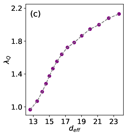
Furthermore, we investigate the condition of equilibration of the spin system which requires the effective dimension of the time-averaged density matrix defined by $d_{\rm eff}=(\sum_{k}|c_{k}|^{4})^{-1}$ to be much larger than $d^{2}_{\rm s}$ ($d_{\rm eff}\gg d^{2}_{\rm s}$) where $d_{\rm s}=2$ is the spin system dimension Linden2009; Gogolin2011. This condition ensures that the initial state is composed of a large number of energy eigenstates so that the bosonic degree of freedom acts as an effective bath coupled to the spin. In Figs. 6(c) and 6(d) we show $d_{\rm eff}$ for different initial spin and Fock states. We see that for all initial states $d_{\rm eff}$ increases with the number of bosons $n$ Clos16. This leads to suppression of the temporal fluctuations and hence equilibration of the spin obsevable which remains close to its time average as is shown in Fig. 6(a). Finally, we note that for large effective dimension $d_{\rm eff}$ the initial local information is spread between large number of eigenstates which increases $\lambda_{Q}(g,\omega,\Delta)$ and thus makes the QR system more chaotic, see Fig. 6(c).

We have shown that the critical QR model exhibits signatures of quantum chaos in the superradiant phase that become more apparent as we approach the effective thermodynamic limit $\eta\rightarrow\infty$. This is most clearly seen in the behaviour of the FOTOC which also quantifies chaos via the quantum Lyuapunov exponent. Furthermore, we investigate the equilibration of the spin degree of freedom in the QR model. We see that the system doesn’t thermalize in general, but exhibits relaxation due to dephasing, characterized by the long-time average of observables that can be described using the diagonal density ensemble. We also have shown that the effective dimension of the time-averaged density matrix can be much larger than the spin system dimension which leads to equilibration of the spin observables.

We thank W. Li for useful discussion. A. V. K. and P. A. I. acknowledges support by the ERyQSenS project, Bulgarian Science Fund Grant No. DO02/3. D.P. acknowledges support from Spanish project PGC2018-094792-B-100(MCIU/AEI/FEDER, EU).

References

- (1) Q. Xie, H. Zhong, M. T. Batchelor, and C. Lee, J. Phys. A: Math. Theor. 50, 113001 (2017).
- (2) J. S. Pedernales, I. Lizuain, S. Felicetti, G. Romero, L. Lamata, and E. Solano, Sci. Rep. 5, 15472 (2015).
- (3) D. Lv, S. An, Z. Liu, J.-N. Zhang, J. S. Pedernales, L. Lamata, E. Solano, and K. Kim, Phys. Rev. X 8, 021027 (2018).
- (4) M. Hwang, R. Puebla, M. B. Plenio, Phys. Rev. Lett. 115, 180404 (2015).
- (5) L. Bakemeier, A. Alvermann, H. Fehske, Phys. Rev. A 85, 043821 (2012).
- (6) M.-L. Cai et al., Nature Commun. 12, 1126 (2021).
- (7) P. Pérez-Fernández et al., Phys. Rev. E 83, 046208 (2011).
- (8) C. Emary, T. Brandes, Phys. Rev. Lett. 90, 044101 (2003).
- (9) C. Emary, T. Brandes, Phys. Rev. E 67, 066203 (2003).
- (10) B. Georgeot, D. Shepelyansky, Phys. Rev. Lett. 81, 5129 (1998).
- (11) R. J. Lewis-Swan, A. Safavi-Naini, J. J. Bollinger, A. M. Rey, Nature Commun. 10, 1581 (2019).
- (12) M. Berry, M. Tabor, Proc. R. Soc. Lond. A 356 375 (1977).
- (13) L. D’Alessio, Y. Kafri, A. Polkovnikov, M. Rigol, Adv. Phys. 65, 239 (2016).
- (14) M. Kuś, Phys. Rev. Lett. 54, 1343 (1985).
- (15) B. Swingle, Nature Phys. 14, 988 (2018).
- (16) S. H. Shenker, D. Stanford, J. High Energ. Phys. 2014, 67 (2014).
- (17) A. Bohrdt, C. B. Mendl, M. Endres, and M. Knap, New J. Phys. 19, 063001 (2017).
- (18) H. Shen, P. Zhang, R. Fan, and H. Zhai, Phys. Rev. B 96, 054503 (2017).
- (19) M. Gärttner, J. G. Bohnet, A.S.-Naini, M. L. Wall, J. J. Bollinger, and A. M. Rey, Nature Phys. 13, 781 (2017).
- (20) K. A. Landsman, C. Figgtt, T. Schuster, N. M. Linke, B. Yoshida, N. Y. Yao, and C. Monroe, Nature 567, 61 (2019).
- (21) M. K. Joshi, A. Elben, B. Vermersch, T. Brydges, C. Maier, P. Zoller, R. Blatt, and C. F. Roos, Phys. Rev. Lett. 124, 240505 (2020).
- (22) A. M. Green, A. Elben, C. H. Alderete, L. K. Joshi, N. H. Nguyen, T. V. Zache, Y. Zhu, B. Sundar, and N. M. Linke, arXiv:2112,02068 (2021).
- (23) J. Li, R. Fan, H. Wang, B. Ye, B. Zeng, H. Zhai, X. Peng, and J. Du, Phys. Rev. X 7, 031011 (2017).
- (24) Z.-H. Sun, J.-Q. Cai, Q.-C. Tang, Y. Hu, and H. Fan, Ann. Phys. (Berlin) 532, 1900270 (2019).
- (25) M. Schmitt, D. Sels, S. Kehrein, A. Polkovnikov, Phys. Rev. B 99, 134301 (2019).
- (26) J. Maldacena, S. Shenker, D. Stanford, J. High Energ. Phys. 2016, 106 (2016).
- (27) A. Bohrdt, C. B. Mendl, M. Endres, M. Knap, New J. Phys. 19, 063001 (2017).
- (28) J. C.-Carlos et al., Phys. Rev. Lett. 122, 024101 (2019).
- (29) A. Keselman, L. Nie, E. Berg, Phys. Rev. B 103, 121111 (2021).
- (30) J. Rammensee, J.-D. Urbina, K. Richter, Phys. Rev. Lett. 121, 124101 (2018).
- (31) Y. Sekino, L. Susskind, J. High Energy Phys. 2008, 065 (2008).
- (32) X. Chen, T. Zhou, arXiv:1804.08655.
- (33) H. Gharibyan, M. Hanada, B. Swingle, M. Tezuka, J. High Energy Phys. 2019, 82 (2019).
- (34) D. Porras, P. A. Ivanov, and F. Schmidt-Kaler, Phys. Rev. Lett. 108, 235701 (2012).
- (35) N. Linden, S. Popescu, A. J. Short, and A. Winter, Phys. Rev. E 79, 061103 (2009).
- (36) C. Gogolin, M. P. Müller, and J. Eisert, Phys. Rev. Lett. 106, 040401 (2011).
- (37) C. Gogolin and J. Eisert, Reports on Progress in Physics 79, 056001 (2016).
- (38) D. Braak, Phys. Rev. Lett. 107, 100401 (2011).
- (39) E. M. Fortes, I. García-Mata, R. A. Jalabert, D. A. Wisniacki, Phys. Rev. E 100, 042201 (2019).
- (40) M. Srednicki, Phys. Rev. E 50, 888 (1994).
- (41) J. Deutsch, Phys. Rev. A 43, 2046 (1991).
- (42) M. Rigol, V. Dunjko, M. Olshanii, Nature 452, 854 (2008).
- (43) G. Clos, D. Porras, U. Warring, and T. Schaetz, Phys. Rev. Lett. 117, 170401 (2016).