Preferred basis of states derived from eigenstate thermalization hypothesis
Abstract
We study the long-time average of the reduced density matrix (RDM) of a central system that is locally coupled to a large environment, under a Schrödinger evolution of the total system. We consider a class of interaction Hamiltonian, whose environmental part satisfies the so-called eigenstate thermalization hypothesis ansatz with a constant diagonal part in the energy region concerned. Relations among elements of the averaged RDM are derived. When steady states of the central system exist, these relations imply the existence of a preferred basis, which is given by the eigenbasis of a renormalized self-Hamiltonian that includes certain averaged impact of the system-environment interaction. Numerical simulations performed for a qubit coupled to a defect Ising chain confirm the analytical predictions.
I Introduction
Properties of small open quantum systems, which are coupled to large quantum environments, have attracted significant attention and been studied extensively in recent decades in various fields of physics Leggett et al. 1987; Breuer et al. 2002; Alicki and Lendi 2007; Breuer et al. 2016; De Vega and Alonso 2017. Such a central system is described by its reduced density matrix (RDM) and may approach a steady state in many situations. For example, it is now well known that the phenomenon of decoherence, due to interactions with huge quantum environments, may happen in such a way that a RDM becomes approximately diagonal on a so-called preferred (pointer) basis of states (PBS) Zurek 1981; Zurek 2003; Schlosshauer 2005; Wiseman and Milburn 2009; Paz and Zurek 1999; Joos et al. 2013. Under pure-dephasing interactions, decoherence has been studied well, with PBS given by eigenbases of self-Hamiltonians Gorin et al. 2004; Albash and Lidar 2015; Weiss 2012. However, under strong interactions and complex environments, with the self-Hamiltonians negligible, PBS may be given by eigenbases of the interaction Hamiltonians Zurek 1981; Gorin et al. 2004.
The situation is much more complicated with a generic dissipative interaction, whose Hamiltonian is not commutable with the central system’s self-Hamiltonian, due to the interplay of decoherence and relaxation. In this generic case, knowledge about PBS is still far from being complete. Under a sufficiently weak interaction and by a first-order perturbation theory, it was found that the system’s eigenbasis is approximately a PBS under a quantum chaotic environment Wang et al. 2008. When the total system’s eigenfunctions possess certain special randomness, a PBS (if existing) is given by the eigenbasis of a renormalized self-Hamiltonian He and Wang 2014. These results are in agreement with a generic expectation for Markovian processes described by Lindblad master equations, as exemplified in solvable models Breuer et al. 2002; Alicki and Lendi 2007; Albash and Lidar 2015. While, when non-Markovian effects due to dynamics of the total system are taken into account, nonnegligible off-diagonal elements of RDM have been found at long times in various spin-boson models on the spin’s energy basis Lee et al. 2012; Addis et al. 2014; Roszak et al. 2015; Zhang et al. 2015; Guarnieri et al. 2018.
In this paper, we go further in the study of properties of steady states of small open systems, by directly computing their long-time averaged RDM under overall Schrödinger evolutions of total systems. A key point of our approach is to consider those environments, for which the environmental parts of the interaction Hamiltonians satisfy the so-called eigenstate thermalization hypothesis (ETH) ansatz Deutsch 1991; Srednicki 1994; Srednicki 1999; Rigol et al. 2008; D’Alessio et al. 2016; Deutsch 2018 and their diagonal elements in the ansatz may be treated as constants within the energy regions of relevance. We are to derive relations among elements of such an averaged RDM for a central system with a number of levels. When steady states exist, these relations imply that the central system should have a PBS, which is given by the eigenbasis of a renormalized self-Hamiltonian that includes certain impact of the system-environment interaction.
The paper is organized as follows. In Sec. II, we specify the systems to be studied. In Sec. III, we derive the above-mentioned relations. Some further discussions are given in Sec.IV. Numerical simulations are presented in Sec. V, to illustrate validity of the analytical predictions for a qubit as the central system and a defect Ising chain as the environment. Finally, conclusions and discussions are given in Sec. VI.
II Setup
In this section, we discuss basic properties of the Hamiltonians of the systems to be studied. We use to denote the central system and use to denote its (large) environment which consists of particles (). Hilbert spaces of and are denoted by and , respectively, with dimensions and . The value of is required to be much smaller than the number of environmental levels that are of relevance effectively to the time evolution.
The Hamiltonian of the total system is written as
| (1) |
where and are self-Hamiltonians of and , respectively, which are obtained in the weak coupling limit, and represents a local interaction Hamiltonian. Normalized eigenstates of the total system are denoted by with energies in the increasing-energy order,
| (2) |
Normalized eigenstates of and of are denoted by and , respectively, with labels and as positive integers starting from . The corresponding eigenenergies are denoted by and , respectively, both in the increasing-energy order,
| (3a) | ||||
| (3b) | ||||
where for brevity we have omitted a superscript for . We use to indicate the energy scope the central system :
| (4) |
We use to indicate the uncoupled Hamiltonian,
| (5) |
Its eigenstates are written as , in short, , satisfying , where . The expansion of a state on the basis given by is written as
| (6) |
with expansion coefficients . For the simplicity in discussion, we consider a product form of , 11 1 Generalization to a generic local interaction Hamiltonian will be briefly discussed in Sec. IV.2.
| (7) |
where and are Hermitian operators acting on the two spaces of and , respectively, and is a parameter for characterizing the coupling strength. Elements of and on and are written as
| (8a) | ||||
| (8b) | ||||
To describe locality of the interaction, we further divide the environment into a small part denoted by and a large part denoted by , such that the system is coupled to only. Then, is written as
| (9) |
where is an operator that acts on the Hilbert space of and indicates the identity operator on the Hilbert space of . 22 2 As a local operator, does not change with the environmental particle number .
Although the exact condition under which the ETH ansatz proposed in Ref.Srednicki 1999 is applicable is still unclear, it is usually expected valid at least for local operators of many-body quantum chaotic systems D’Alessio et al. 2016; Deutsch 2018. Here, we assume that this ansatz is applicable to the operator . According to this hypothesis, (1) diagonal elements on average vary slowly with the eigenenergy ; (2) fluctuations of possess certain random feature and are very small, scaling as , where is proportional to the particle number of and is related to the micro-canonical entropy in a semiclassical treatment; and (3) off-diagonal elements with behave in a way similar to fluctuations of Deutsch 1991; Srednicki 1994; Rigol et al. 2008; Srednicki 1999; D’Alessio et al. 2016; Garrison and Grover 2018. These predictions are written in the following concise form, usually referred to as the ETH ansatz,
| (10) |
where , , is a slowly varying function of , is some smooth function, and indicate random variables with a normal distribution (zero mean and unit variance). 33 3 Certain correlations among have been observed numerically in some chaotic systems Wang et al. 2022, but, we do not discuss this possibility in this paper.
Analytical expressions of the functions and are still lacking. Numerically, three regimes have been observed for with respect to the order of per-site energy denoted by , provided that lies in the central region of the spectrum D’Alessio et al. 2016; De Vega and Alonso 2017. That is, for , it shows a plateau with a height proportional to and a width proportional to Rigol et al. 2008; Khatami et al. 2013; for large , it decays exponentially; and, for , it is proportional to in diffusive one-dimensional systems Abanin et al. 2015; Mukerjee et al. 2006; Brenes et al. 2020a; LeBlond et al. 2020.
For the simplicity in discussion, we set the initial state of the total system at a time as a pure state with a product form, 44 4 Discussions to be given below may be generalized, in a straightforward way, to a generic initial state written as , if all the environmental states lie in the same energy shell in Eq.(14). that is,
| (11) |
Here, indicates an arbitrary normalized state of the central system , written as
| (12) |
and is an arbitrary environmental state that lies within an energy shell denoted by ,
| (13) |
The energy shell is centered at an energy and has a width , 55 5 See Sec.III.4 for a discussion about restriction to the width . namely,
| (14) |
III Main result
In this section, we derive the main result of this paper, as relations among elements of the long-time averaged RDM. Specifically, we give some formal discussions in Sec.III.1, then, in Sec.III.2, derive an upper bound to the environmental energy region, which is of relevance effectively to the wave function at all times. The main result is derived in Sec.III.3 and properties of a main condition used in it are discussed in Sec.III.4.
III.1 Preliminary discussions
The total system undergoes a Schrödinger evolution,
| (15) |
We write in the following expansion with respect to the central system’s states ,
| (16) |
and call the environmental branches of . These branches, as vectors in the environmental Hilbert space, are written as
| (17) |
and are usually not normalized. Under the initial condition in Eq.(11), it is direct to find that
| (18) |
and
| (19) |
where indicate operators that act on the Hilbert space of the environment, as defined below,
| (20) |
By definition, the RDM of the system , denoted by , is given by , where . It is easy to check that elements of the RDM on the basis , namely , have the following expression,
| (21) |
Making use of Eq.(19), after some deviation, one finds that the elements satisfy the following equation (see Appendix A),
| (22) |
where
| (23a) | |||||
| (23b) | |||||
Here, indicate -number quantities defined below,
| (24) |
and, from them, we define the following operator,
| (25) |
It is easy to check that and have the following concise expressions,
| (26a) | ||||
| (26b) | ||||
where indicates the transposition operator of , which is defined on the eigenbasis of .
We use an overline to indicate the long-time average of a term. For example, the long-time average of the RDM is written as ,
| (27) |
Clearly, in the case that a steady state of the RDM exists, it is given by . Since the elements have bounded values, the long-time average of must be zero, i.e., . Then, Eq.(22) gives that
| (28) |
Substituting the explicit expressions of and in Eq.(23) into Eq.(28), one finds the following formal relation for the long-time averaged RDM:
| (29) |
It is straightforward to check that a concise form of Eq.(29) is written as
| (30) |
III.2 Effective environmental energy region
In this section, we discuss an environmental energy region, within which all the branches effectively lie for all the times , and indicate it by . We do not need to find the smallest one of this type of region. Instead, we consider a region that has the following simple form,
| (31) |
centered at the initial center and with a width .
Below, we derive an expression for , as an upper bound to the width of the energy region that effectively contains all . For this purpose, we need to analyze the components ,
| (32) |
which is directly obtained by making use of Eqs.(11)-(13) and (15)-(17). Initially, with at , due to correlations among the terms of of different indices , which originate from the completeness of the states as a basis in the total Hilbert space, nonzero values of the rhs of Eq.(32) are restricted within the initial energy region . With increase of the time , the phases gradually destroy the above-mentioned correlations and, as a result, the energy region that is effectively occupied by expands. Cutting all the correlations by taking an absolute value for each summed term on the rhs of Eq.(32), one gets an upper bound to :
| (33) |
When using the rhs of Eq.(33) to get an upper bound to the environmental energy region that effectively contains , exact values of the nonzero coefficients and are not important. Hence, we may focus on the values of . In particular, for the eigenfunction (EF) of each state , what is of relevance is its main-body region, within which the main population lie up to a small error indicated by . Energetically, such a main-body region consists of those uncoupled states , whose energies are around the exact energy within a scope which we indicate by . More exactly, the set of the indices of these uncoupled states, indicated by , is written as
| (34) |
Then, the main-body region of the EF satisfies the following requirement,
| (35) |
where “” means that the set is chosen such that the left hand side of Eq.(35) is the closest to its right hand side.

For a product to give a nonnegligible contribution to the rhs of Eq.(33), both of the two basis states and should lie in the main-body region of . As as result, the expansion from to should be influenced mainly by two factors: widths of main-body regions of the EFs and the central system’s energy differences. We use to indicate the maximum value of for those states that are of relevance to the time evolution of the initial state. Then, noting that in Eq.(4) gives the maximum of , we find the following expression of ,
| (36) |
as illustrated in Fig.1.
Two remarks are in order: (1) At , the real width is just , smaller than . (2) When the states are sufficiently coupled by the interaction, it is possible for in Eq.(36) to be close to the width of the energy region that is really occupied.
III.3 Relations among elements of averaged RDM
In this section, we derive the main result, as relations that the elements of satisfy. To this end, let us expand the environmental branches as,
| (37) |
with expansion coefficients . Substituting Eq.(37) into Eqs.(21) and (24), taking the long-time average, and making use of the fact that all the environmental branches effectively lie within the energy region , one finds the following expressions of and ,
| (38) | ||||
| (39) |
Substituting the ETH ansatz (10) into Eq.(39), one gets that
| (40) |
where indicates a fluctuation term, given by
| (41) |
Generically, the two operators and do not have a simple relationship. One key observation made here is that they may possess a simple relationship, if the function is approximately a nonzero constant within the energy shell . More exactly, the condition is that
| (42) |
where is a parameter much smaller than , with (even in the limit of ), and indicates the maximum difference between and within :
| (43) |
To show the above-mentioned relationship, we note that, when the condition in Eq.(42) is satisfied, Eqs.(38) and (40) imply that
| (44) |
or, equivalently,
| (45) |
where is a fluctuation operator,
| (46) |
From the rhs of Eq.(41), one sees three factors that influence the -dependence of . The first one is the exponential decay of , with . The second factor is given by the unknown ETH-ansatz function , for which numerical simulations show a polynomial increase of , with in some (diffusive one-dimensional) systems Luitz and Lev 2016; D’Alessio et al. 2016. The third factor lies in the summation over the indices and and the long-time average term . As shown in Appendix B, due to the randomness of , contribution from the third factor is negligible compared with the first factor. (See Eq.(97) for an upper bound to the norm of .) Therefore, the -scaling behavior of the fluctuation operator is dominated by the exponential decay term . Due to this exponential decay, as well as the fact that in the limit of large and that each RDM has a unit trace, one gets that
| (47) |
Then, Eq.(45) gives the following relation between the two operators of and :
| (48) |
The main result of this paper is obtained by substituting Eq.(48) into Eq.(30),
| (49) |
which holds under the condition of Eq.(42) and at sufficiently large . Here, is a renormalized self-Hamiltonian of the central system, defined by
| (50) |
which includes certain averaged impact of the system-environment interaction. From Eq.(49), one sees that, if a PBS exists, it should be given by the eigenbasis of the renormalized self-Hamiltonian . Writing Eq.(49) explicitly, one gets that
| (51) |
This gives relations among elements of the averaged RDM for and relations for .
As an illustration of the above result, let us consider a nondegenerate two-level system (TLS), with . From Eq.(51) with , one gets that
| (52) |
where
| (53) |
The quantity gives a relative measure for the strength of dephasing, while, gives a relative measure for the strength of relaxation (dissipation). Meanwhile, in the case of , one gets that
| (54) |
which implies approximate realness of the product .
III.4 - and -relevance to the condition (42)
In this section, we discuss relevance of the particle number to Eq.(42), a main prerequisite for the above-derived main result, as well as relevance of the interaction strength . 66 6 One may note that Eq.(42) is always satisfied, in the case that EFs of the quantum chaotic environment may be effectively described by the random matrix theory (RMT). In fact, in this case, is a constant, given by D’Alessio et al. 2016. Basically, Eq.(42) requires that the environmental energy shell should be “sufficiently narrow”, such that the function may be approximately taken as a constant within it, compared with its nonzero central value . Below, we give a detailed discussion of the exact meaning of “being sufficiently narrow”.
III.4.1 Relevance of the particle number N
Relevance of to Eq.(42) comes mainly from two aspects: the width of in Eq.(36) and the ETH-ansatz function . The width contains three terms. Clearly, , the central system’s energy scope, is -independent. The -dependence of is usually determined according to the problem at hand, particularly, to quantities of final interest; e.g., it may be taken as a constant, or as some polynomial function of .
The situation with , the maximum width of relevant EFs of the total system on the uncoupled energy basis, is more complicated. In fact, presently, still not much is known analytically about widths of the EFs. It seems reasonable to assume that with some parameter the value of which may be model-dependent. By a first-order perturbation-theory treatment to long tails of EFs in certain model, it was found that Wang 2012; while, a study of higher-order contributions is still under investigation Wang et al. by making use of a semiperturbative theory Wang and Wang 2019; Wang et al. 1998; Wang 2000; Wang 2002.
The ETH ansatz does not assume any specific form of the function . According to numerical simulations with the help of some analytical analysis Kim et al. 2014; Brenes et al. 2020a; D’Alessio et al. 2016; Brenes et al. 2020b, was found approximately a function of per-site energy,
| (55) |
where is some smooth function of , independent of . Then, Taylor’s expansion gives that
| (56) |
where indicates the derivative of and represents the second and higher order terms of the expansion.
To be specific, let us discuss a case, in which the initial width increases slower than such that
| (57) |
This case may be met quite often practically. Note that Eq.(57) does not really require narrowness of the initial shell ; e.g., it holds for with a parameter . Then, as long as for , Eq.(57) implies that
| (58) |
This implies that the ratio should approach zero in the limit of large for . If , then, according to Eq.(56), the difference is approximately given by the first-order term at sufficiently large . As a consequence, is approximately a linear function within and in Eq.(43) is written as
| (59) |
One sees that, as long as has a finite upper bound, in the limit of . Otherwise, i.e., if , one may consider the second-order term (if nonzero) in Eq.(56) and, following arguments similar to those given above, reach the same conclusion. Similar arguments also apply, when higher-order terms dominate. Therefore, for systems with , under an initial condition satisfying Eq.(57), the condition (42) is usually fulfilled at sufficiently large .
III.4.2 Relevance of the interaction strength
Among the three terms of , , and in , only the EF width depends on the interaction strength . As is well known, usually, increases with increasing , when other parameters in the total Hamiltonian are fixed. It is reasonable to expect that dependence of on the pair of may behave in a quite complicated way. A full understanding of this behavior is beyond the scope of this investigation. Below, for the sake of clearness in discussion, we usually consider a fixed value of when discussing influence of .
To study influence of the interaction strength on the condition in Eq.(42), let us consider a case in which Eq.(42) is satisfied at with . For example, one has such a case, if the initial shell is sufficiently narrow and the value of is sufficiently small. With increase of from , the value of increases due to the increase of . At a small , the width is still small and, as a result, Eq.(42) is also satisfied.
When the value of increases beyond some regime, usually, it is possible for to become sufficiently large such that Eq.(42) gradually becomes invalid. Note that the width has no upper bound, because it should increase (approximately) linearly with when the interaction Hamiltonian dominates in the total Hamiltonian. To be quantitative, related to breakdown of Eq.(42), one may consider a value of , indicated as , at which the value of first reaches when increases from . Making use of Eqs.(59) and (36), from Eq.(42) one gets that
| (60) |
Two properties are seen from Eq.(60): (1) Since the width usually increases with increasing , for systems with , the value of may increase with increasing ; and, (2) should increase with decreasing , if other parameters are fixed.
IV Further discussions
In this section, we discuss two situations, in which some modified versions of the RDM relations given in the main result still hold when some restrictions used above are loosened. In Sec.IV.1, we derive RDM relations in the weak coupling limit, without the restriction of Eq.(42). In Sec.IV.2, we show that the main result may be generalized to a generic local interaction Hamiltonian.
IV.1 Offdiagonal elements at very weak couplings
In this section, in the weak coupling limit of , without using the condition in Eq.(42), we derive an expression for offdiagonal elements of the averaged RDM of nondegenerate levels, by employing a first-order perturbation treatment. In this limit, diagonal elements of RDM keep approximately constants, directly given by the initial condition:
| (61) |
To be specific, below, we consider two arbitrary nondegenerate levels of the central system , indicated by and with . The zeroth-order branches, denoted by , are computed by the Schrödinger evolution of the initial state under the uncoupled Hamiltonian . Noting Eq.(11), one directly gets that
| (62) |
Substituting Eq.(62) into Eq.(21) and noting that , one sees that has a vanishing zeroth-order term.
The zeroth-order term of , indicated as , is computed by substituting Eq.(62) into Eq.(24) and taking the long-time average. Noting that the chaotic environment has a nondegenerate spectrum, direct computation gives that 77 7 For an environment that possesses a degenerate spectrum, one may divide the set of those labels , for which , into subsets according to the degeneracy. We denote the subsets by with a label , such that for all . Then, it is easy to find that (63)
| (64) |
where
| (65) |
Now, we compute the first-order term of . For this purpose, let us rewrite Eq.(29) as follows,
| (66) |
Substituting the above-obtained zeroth-order terms into the rhs of Eq.(66), one gets the following expression of up to the first-order term:
| (67) |
Finally, we compare two results obtained above, Eq.(67) and Eq.(52), the latter of which is a TLS case of the main result in Eq.(51). The two results were gotten under different conditions: Eq.(67) was derived merely under the condition of very weak coupling, while, Eq.(51) was derived under a condition that includes three requirements : ETH ansatz in Eq.(10), Eq.(42), and largeness of . We would remark that the above two conditions are sufficient conditions for the corresponding results, but not necessary conditions. For example, it is possible for Eq.(52) to hold in some cases, even when Eqs.(10) and (42) are not fulfilled. In addition, none of the two conditions includes the other.
To show consistency of the above two results, let us consider a case in which both conditions are satisfied. In fact, under Eqs.(10) and (42), it is easy to see that in Eq.(65) satisfies that . Then, in the weak coupling limit with Eq.(61), Eq.(67) is written as
| (68) |
Clearly, Eq.(68) gives the same prediction as Eq.(52) in this case.
IV.2 A generic interaction
In this section, we give a brief discussion for a generic local interaction Hamiltonian , which is written as a sum of direct-product terms. Suppose that there are such terms, with the subscript “LIT” standing for “local interaction terms”. Then, is written as
| (69) |
where are parameters and are local operators of the environment. The operators are assumed to satisfy the ETH ansatz, with functions , respectively. For such a generic , the operator in Eq.(25) is written as
| (70) |
where
| (71) |
Following arguments similar to those given in Sec.III, with appropriate generalizations, one may study the long-time average of this generic operator and get similar results. More exactly, the main generalization is that Eq.(42) is now written as
| (72) |
where and
| (73) |
The final result is that, at a sufficiently large ,
| (74) |
where
| (75) |
V Numerical tests
In this section, we present numerical simulations that have been performed for checking analytical predictions given above. Specifically, we discuss the employed model and analytical predictions in Sec.V.1, and discuss numerical simulations in Sec.V.2.
V.1 The model
In numerical simulations, we employ a TLS as the central system and one defect Ising chain as the environment . The TLS has a self-Hamiltonian written as
| (76) |
where is a parameter and indicates the -component Pauli matrix divided by .
The defect Ising chain is composed of a number of -spins lying in an inhomogeneous transverse field, whose Hamiltonian is written as
| (77) |
where and indicate Pauli matrices divided by at the -th site. Here, , , , and are parameters, which are adjusted such that the defect Ising chain is a quantum chaotic system. That is, for levels not close to edges of the energy spectrum, the nearest-level-spacing distribution is close to the Wigner-Dyson distribution , the latter of which is almost identical to the prediction of RMT Haake 2013; Casati et al. 1980; Bohigas et al. 1984. Exact values of the parameters used are , , and ; and is between and . In our numerical computation of EFs, the periodic boundary condition was implied and the so-called Krylov-space method was used.
The TLS is coupled to the -th spin of the defect Ising chain. We have studied two specific forms of the local interaction Hamiltonian, indicated as and ,
| (78a) | ||||
| (78b) | ||||
Their difference lies in that the TLS part of has no overlap with in Eq.(76), while, has some. According to Eqs.(4) and (53), one finds that , and for , and and for . Numerically, we have checked that the ETH ansatz is applicable to local operators in the defect Ising chain (see Appendix C).

Below, we discuss predictions for properties of the long-time-averaged RDM element of the TLS, which are given by analytical results of previous sections. We discuss in the increasing order of the interaction strength .
(1) Regime of very small (weak coupling limit).
As discussed in Sec.IV.1,
should satisfy Eq.(67) at very small .
Since the ETH ansatz is applicable to the defect Ising chain, when Eq.(42) is satisfied,
this prediction coincides with Eq.(52),
which is the TLS case of the main result in Eq.(51).
(2) Regime of small but not very small .
(a) Eq.(42) being valid at .
In this case, Eq.(42) is also valid at small .
As a result, should satisfy the main prediction Eq.(52) at sufficiently large .
(b) Eq.(42) being invalid at .
In this case, there is no definite analytical prediction for beyond the weak coupling limit.
(3) Regime of below with Eq.(42) valid.
As discussed in Sec.III.4.2, Eq.(52) is applicable for below .
The value of , which satisfies Eq.(60), is expected to increase with increasing
if ,
while, increase with decreasing .
As discussed previously, Eq.(42) belongs to a sufficient, but not necessary, condition for validity of Eq.(52). This implies that Eq.(52) might be useful even beyond . To directly study validity of Eq.(52), one may compute the value of , indicated by , at which the relative error first reaches some small parameter indicated by when increases from ,
| (79) |
where indicates the exact value of the RDM element and is for the prediction of Eq.(52).
We have no definite analytical prediction for behaviors of . It seems reasonable to expect that, at least in some cases, may show some behavior qualitatively similar to that of as discussed above in predication (3).
V.2 Numerical simulations
We have numerically checked the above predictions for various values of the parameters concerned. The environmental initial state was taken as a typical state within an energy shell , which is given by and .
Two values of has been studied, namely, and . For , we found that at and , implying invalidity of Eq.(42). With changed to , we found , implying validity of Eq.(42). In both cases, .
Variations of versus the interaction strength are shown in Fig.2, for the above-mentioned two values of and for the two interaction Hamiltonians in Eq.(78). One sees that there is in fact no qualitative difference between results for the two interaction Hamiltonians. In the computation of the rhs of Eq.(52), exact values of and were used. In agreement with prediction, both the main result of Eq.(52) (solid lines) and the weak-coupling prediction of Eq.(67) (dashed-dotted lines) work well at very small , more exactly, at around and smaller. Consistently, the mean nearest-level spacing of the total system was found about in the considered energy region at .
With increased above , as expected, the weak-coupling predictions (dashed-dotted lines in blue) gradually deviate from the exact values of (triangles). Meanwhile, consistent with the prediction of (2)(a), for with Eq.(42) valid, predictions of Eq.(52) (solid lines in red) remain close to the triangles, up to . It is of interested to note that, even in the case of with Eq.(42) unsatisfied, predictions of Eq.(52) remains valid up to .
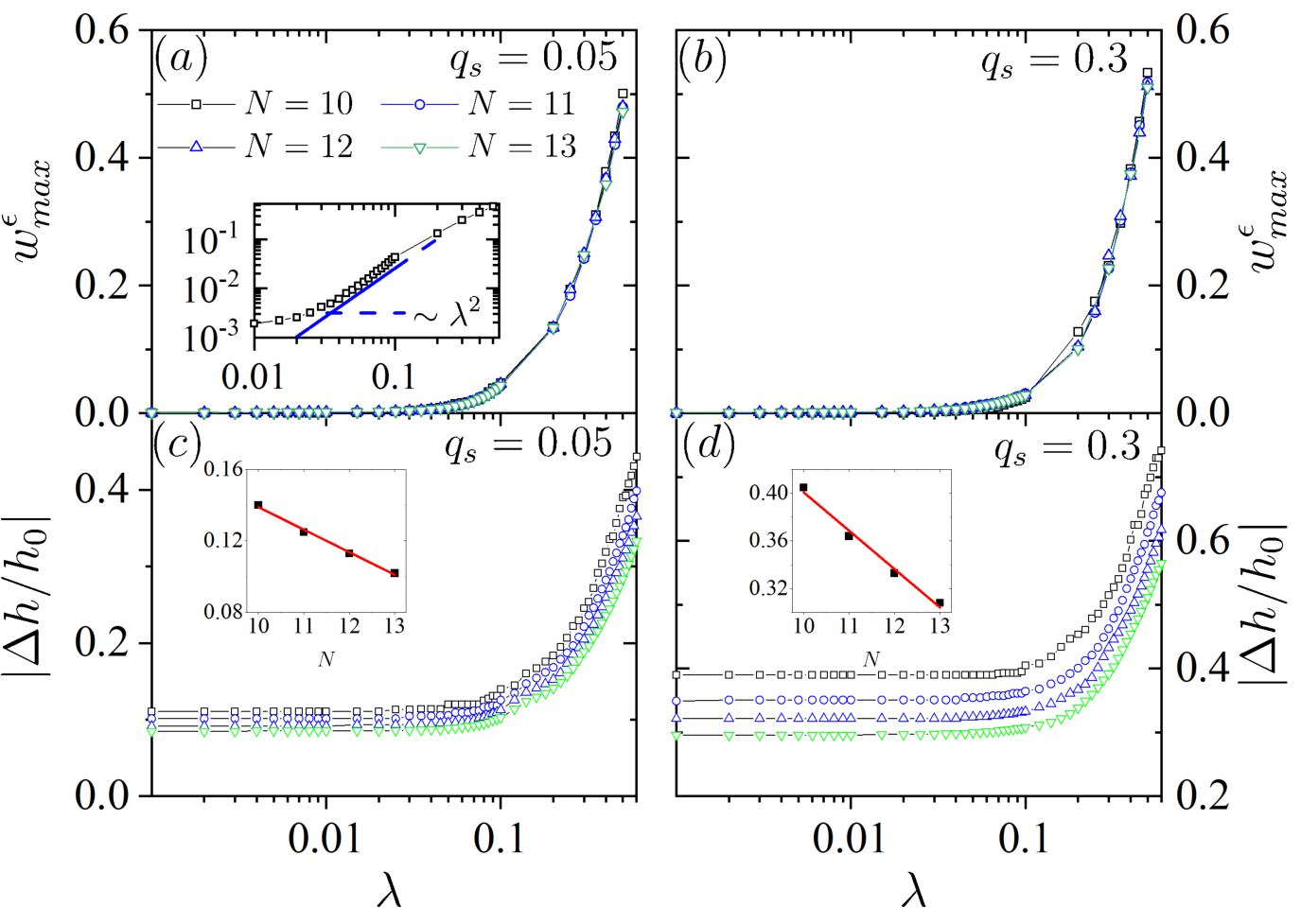
To get further understanding for the above-discussed behaviors of , we have studied variation of the maximum width , which is responsible to the -dependence of the width of , versus , as well as variation of (Fig.3). It is seen that, at and , the value of keeps small for small and begin to increase fast around ; and, consistently, (triangles down) behaves in a similar way. Similar behaviors are seen at and , except that is already large at .
We have also studied impact of the particle number . As seen in Fig.3, the width is almost independent of for from to , which implies a negligible value of , i.e., . Meanwhile, the value of decreases with increasing , in agreement with a prediction of Eq.(59) that may scale as at a fixed value of [insets of Fig.3(c) and (d)]. Moreover, with , according to prediction (3), may increase with increasing ; in other words, Eq.(52) may work better at larger , which is seen by comparing Fig.4 and Fig.2.
Finally, we discuss numerically obtained values of for validity of Eq.(42) and values of for practical use of Eq.(52). The values of may be directly gotten from Fig.3. Taking , we found that Eq.(42) is valid for no value of at and , which is indicated as in Table 1; and, similarly, for and . Thus, has definite values only at and . If the restriction of is loosed a little, i.e., if taking larger than but still small (e.g., ), may have definite values in more cases, which is clear from Fig.3(c). In all the cases in which has definite values for Eq.(42), we found that larger value of corresponds to larger value of , meanwhile, larger value of corresponds to smaller value of , in agreement with prediction (3).
Values of were computed by making use of Eq.(79) with . At with Eq.(42) valid, as seen in Table 1, increases with increasing and is close to for . But, at with Eq.(42) invalid, shows a quite complicated behavior; more exactly, it does not increase monotonically with and is unexpectedly large at .
| None | 0.04 | 0.07 | 0.1 | |
| None | None | None | None | |
| 0.025 | 0.04 | 0.07 | 0.1 | |
| 0.1 | 0.015 | 0.025 | 0.015 |

VI Conclusions and discussions
In this paper, the long-time averaged RDM has been studied for a generic small central system with levels, which is locally coupled to a large many-body chaotic environment , with the total system undergoing a Schrödinger evolution. Beside largeness of the particle number of , the only restriction is that the environmental part of the interaction Hamiltonian satisfies the ETH ansatz, with the diagonal term in the ansatz [namely the function ] approximately a constant within the energy region of relevance. For such a total system, on the eigenbasis of the central system, approximate relations have be derived among elements of its steady states (if existing).
The above-discussed relations imply that the steady RDM should be commutable with a renormalized Hamiltonian of the central system, which includes certain averaged impact of the system-environment interaction. As a consequence, decoherence happens on the eigenbasis of the renormalized Hamiltonian, even under a system-environment interaction that is dissipative for the original Hamiltonian , and leads to a PBS given by the eigenbasis of . This enriches analytical knowledge about PBS for systems under nonweak and dissipative system-environment interactions, which had been previously observed numerically in some specific models (see, e.g., Ref.Wang et al. 2012). 88 8 We would note a difference between the type of models studied in this paper and the spin-boson models used in Refs.Lee et al. 2012; Addis et al. 2014; Roszak et al. 2015; Zhang et al. 2015; Guarnieri et al. 2018. That is, in a spin-boson model, the environment (the bosons) is not a quantum chaotic system and the ETH ansatz is usually inapplicable. Due to this difference, even if a PBS may exist in a spin-boson model, the mechanism should be quite different from that discussed in this paper. Moreover, results of this paper give an explicit way of constructing renormalized Hamiltonian for PBS.
In fact, renormalized Hamiltonian is also used in a standard master-equation approach to RDM. There, at an initial stage before the derivation begins, the self-Hamiltonian of the central system is taken as certain renormalized Hamiltonian, which we indicate as with “mas” standing for “master equation”, given by , where denotes a thermal state of the environment. Under the ETH ansatz and the condition in Eq.(42), has almost the same expression as in Eq.(50), if the state lies effectively within the energy shell .
However, there is a big difference between the physical meanings of and . In fact, in our approach, the operator is derived by faithfully taking the long-time average over the overall Schrödinger evolution; and it indicates the existence of a PBS, if the RDM may approach a steady state. While, in the master-equation approach, the operator is mainly employed for the sake of convenience in derivation, though with deep physical intuition lying behind it. Only after a certain type of analytical solution to a derived master equation is found, which is usually a hard task except in some special models, could it become clear whether may indeed be of relevance to a PBS. Moreover, as an approach based a perturbative treatment, validity of the master-equation approach at long times is a subtle issue.
Finally, we would mention that, beside the field of decoherence, results of this paper may also be useful in other fields in which properties of steady states of small and open quantum systems are of relevance, such as quantum thermodynamics Binder et al. 2019; Goold et al. 2016; Wang 2012; Wang 2018.
Acknowledgements.
This work was partially supported by the Natural Science Foundation of China under Grant No. 11535011, 11775210, and 12175222. JW are supported by the Deutsche Forschungsgemeinschaft (DFG) within the Research Unit FOR 2692 under Grant No. 397107022 (GE 1657/3-2).Appendix A Derivation of Eq.(22)
In this appendix, we derive Eq.(22). Using Eq.(21), the time evolution of the RDM is written as
| (80) |
where
| (81a) | ||||
| (81b) | ||||
Making use of Eq.(19), one finds that
| (82) |
From Eqs.(7) and (20), one gets that
| (83) |
Then, we write Eq.(82) as,
| (84) |
Noting Eqs.(21) and (24), the above equality gives that
| (85) |
Similarly, one finds
| (86) |
Putting the above results together, one gets Eq.(22).
Appendix B Scaling of the fluctuation operator
In this appendix, we show that the main -scaling behavior of the fluctuation operator ,
| (87) |
is an exponential decay with increasing . For this purpose, let us compute the Frobenius norm of ,
| (88) |
Making use of Eq.(41), direct derivation shows that
| (89) |
Note that and . To proceed, let us discuss the statistical average of , taken over the random variables , which is indicate by . This averaging procedure results in that Murthy and Srednicki 2019; D’Alessio et al. 2016
| (90) |
and, as a consequence,
| (91) |
To compute , we make use of the fact that . This gives that
| (92) |
Note that the environment , as a quantum chaotic system, has a nondegenerate spectrum. Under a generic system-environment interaction, the spectrum of the total system is nondegenerate, too. Then, one has and, as a result,
| (93) |
This gives that
| (94) |
Then, making use of the completeness of the basis of and that of , one gets that
| (95) |
where is the so-called participation function of the initial state , defined by
| (96) |
As is known, gives a measure to the localization length, i.e., to the number of those levels that are effectively occupied by the state . For a large environment and an initial shell not extremely narrow, the value of is large.
Substituting Eq.(95) into Eq.(91), we get an upper bound to the averaged norm , i.e.,
| (97) |
Since the averaging procedure does not change the -scaling behavior of the norm and the exponential-decay term already exists in the exact expression of in Eq.(41), from Eq.(97) one sees that the -scaling behavior of fluctuation operator should be dominated by the exponential decay .
Appendix C Verification of ETH ansatz

Due to the hypothesis feature of the ETH ansatz in Eq.(10), we have checked its validity in the model employed in this paper. We did this for the two local operators and at the site in the defect Ising chain.

Diagonal ETH.— Let us first discuss predictions of Eq.(10) for diagonal elements of local observables. Expectation values of the two local observables,
| (98) |
are plotted in Fig.C. 1. It is seen that, in agreement with ETH, the diagonal elements fluctuate around certain slowly varying function and the fluctuations decrease with increasing the particle number . Note that the horizontal axis is labeled by . For , the values of are close to zero, while, for , most of are notably larger than zero.
To study quantitatively the fluctuations of , we have computed the standard deviations ,
| (99) |
where
| (100) |
As seen in Fig. C. 2 (a), the fluctuation decays exponentially with the increase of , as predicted by the term in the second part on the rhs of Eq.(10). Moreover, in agreement with the prediction of ETH, the distributions of are close to the Gaussian form [Fig. C. 3 (a) and (b)].


Off-diagonal ETH.— Next, we discuss the offdiagonal elements . In agreement with the prediction of ETH, the probability distributions of have a Gaussian form [Fig. C. 3 (c) and (d)], where are the standard deviations for the offdiagonal elements,
| (101) |
These standard deviations also decay exponentially with the increase of [Fig. C. 2 (b)].
To get some knowledge about shapes of the function , which lacks an analytical expression, numerical simulations have been performed for locally averaged values of and for off-diagonal elements. As seen in Fig.C. 4, the function shows a size-independent feature, with an exponential-type decay at large .
References
- Leggett et al. (1987) A. J. Leggett, S. Chakravarty, A. T. Dorsey, M. P. Fisher, A. Garg, and W. Zwerger, Dynamics of the dissipative two-state system, Reviews of Modern Physics 59, 1 (1987).
- Breuer et al. (2002) H.-P. Breuer, F. Petruccione, et al., The theory of open quantum systems (Oxford University Press on Demand, 2002).
- Alicki and Lendi (2007) R. Alicki and K. Lendi, Quantum dynamical semigroups and applications, Vol. 717 (Springer, 2007).
- Breuer et al. (2016) H.-P. Breuer, E.-M. Laine, J. Piilo, and B. Vacchini, Colloquium: Non-markovian dynamics in open quantum systems, Reviews of Modern Physics 88, 021002 (2016).
- De Vega and Alonso (2017) I. De Vega and D. Alonso, Dynamics of non-markovian open quantum systems, Reviews of Modern Physics 89, 015001 (2017).
- Zurek (1981) W. H. Zurek, Pointer basis of quantum apparatus: Into what mixture does the wave packet collapse?, Physical review D 24, 1516 (1981).
- Zurek (2003) W. H. Zurek, Decoherence, einselection, and the quantum origins of the classical, Reviews of modern physics 75, 715 (2003).
- Schlosshauer (2005) M. Schlosshauer, Decoherence, the measurement problem, and interpretations of quantum mechanics, Reviews of Modern physics 76, 1267 (2005).
- Wiseman and Milburn (2009) H. M. Wiseman and G. J. Milburn, Quantum measurement and control (Cambridge university press, 2009).
- Paz and Zurek (1999) J. P. Paz and W. H. Zurek, Quantum limit of decoherence: Environment induced superselection of energy eigenstates, Physical Review Letters 82, 5181 (1999).
- Joos et al. (2013) E. Joos, H. D. Zeh, C. Kiefer, D. J. Giulini, J. Kupsch, and I.-O. Stamatescu, Decoherence and the appearance of a classical world in quantum theory (Springer Science & Business Media, 2013).
- Gorin et al. (2004) T. Gorin, T. Prosen, T. Seligman, and W. Strunz, Connection between decoherence and fidelity decay in echo dynamics, Physical Review A 70, 042105 (2004).
- Albash and Lidar (2015) T. Albash and D. A. Lidar, Decoherence in adiabatic quantum computation, Physical Review A 91, 062320 (2015).
- Weiss (2012) U. Weiss, Quantum dissipative systems, Vol. 13 (World scientific, 2012).
- Wang et al. (2008) W.-g. Wang, J. Gong, G. Casati, and B. Li, Entanglement-induced decoherence and energy eigenstates, Physical Review A 77, 012108 (2008).
- He and Wang (2014) L. He and W.-g. Wang, Statistically preferred basis of an open quantum system: Its relation to the eigenbasis of a renormalized self-hamiltonian, Physical Review E 89, 022125 (2014).
- Lee et al. (2012) C. K. Lee, J. Cao, and J. Gong, Noncanonical statistics of a spin-boson model: Theory and exact monte carlo simulations, Physical Review E 86, 021109 (2012).
- Addis et al. (2014) C. Addis, G. Brebner, P. Haikka, and S. Maniscalco, Coherence trapping and information backflow in dephasing qubits, Physical Review A 89, 024101 (2014).
- Roszak et al. (2015) K. Roszak, R. Filip, and T. Novotnỳ, Decoherence control by quantum decoherence itself, Scientific reports 5, 1 (2015).
- Zhang et al. (2015) Y.-J. Zhang, W. Han, Y.-J. Xia, Y.-M. Yu, and H. Fan, Role of initial system-bath correlation on coherence trapping, Scientific reports 5, 1 (2015).
- Guarnieri et al. (2018) G. Guarnieri, M. Kolář, and R. Filip, Steady-state coherences by composite system-bath interactions, Physical review letters 121, 070401 (2018).
- Deutsch (1991) J. M. Deutsch, Quantum statistical mechanics in a closed system, Physical review a 43, 2046 (1991).
- Srednicki (1994) M. Srednicki, Chaos and quantum thermalization, Physical review e 50, 888 (1994).
- Srednicki (1999) M. Srednicki, The approach to thermal equilibrium in quantized chaotic systems, Journal of Physics A: Mathematical and General 32, 1163 (1999).
- Rigol et al. (2008) M. Rigol, V. Dunjko, and M. Olshanii, Thermalization and its mechanism for generic isolated quantum systems, Nature 452, 854 (2008).
- D’Alessio et al. (2016) L. D’Alessio, Y. Kafri, A. Polkovnikov, and M. Rigol, From quantum chaos and eigenstate thermalization to statistical mechanics and thermodynamics, Advances in Physics 65, 239 (2016).
- Deutsch (2018) J. M. Deutsch, Eigenstate thermalization hypothesis, Reports on Progress in Physics 81, 082001 (2018).
- Garrison and Grover (2018) J. R. Garrison and T. Grover, Does a single eigenstate encode the full hamiltonian?, Physical Review X 8, 021026 (2018).
- Wang et al. (2022) J. Wang, M. H. Lamann, J. Richter, R. Steinigeweg, A. Dymarsky, and J. Gemmer, Eigenstate thermalization hypothesis and its deviations from random-matrix theory beyond the thermalization time, Physical Review Letters 128, 180601 (2022).
- Khatami et al. (2013) E. Khatami, G. Pupillo, M. Srednicki, and M. Rigol, Fluctuation-dissipation theorem in an isolated system of quantum dipolar bosons after a quench, Physical review letters 111, 050403 (2013).
- Abanin et al. (2015) D. A. Abanin, W. De Roeck, and F. Huveneers, Exponentially slow heating in periodically driven many-body systems, Physical review letters 115, 256803 (2015).
- Mukerjee et al. (2006) S. Mukerjee, V. Oganesyan, and D. Huse, Statistical theory of transport by strongly interacting lattice fermions, Physical Review B 73, 035113 (2006).
- Brenes et al. (2020a) M. Brenes, T. LeBlond, J. Goold, and M. Rigol, Eigenstate thermalization in a locally perturbed integrable system, Physical review letters 125, 070605 (2020a).
- LeBlond et al. (2020) T. LeBlond, D. Sels, A. Polkovnikov, and M. Rigol, Universality in the onset of quantum chaos in many-body systems, arXiv preprint arXiv:2012.07849 (2020).
- Luitz and Lev (2016) D. J. Luitz and Y. B. Lev, Anomalous thermalization in ergodic systems, Physical review letters 117, 170404 (2016).
- Wang (2012) W.-g. Wang, Statistical description of small quantum systems beyond the weak-coupling limit, Physical Review E 86, 011115 (2012).
- (37) W.-g. Wang, Q.-c. Li, M. Yuan, and J. Wang, in preparation.
- Wang and Wang (2019) J. Wang and W.-g. Wang, Convergent perturbation expansion of energy eigenfunctions on unperturbed basis states in classically-forbidden regions, Journal of Physics A: Mathematical and Theoretical 52, 235204 (2019).
- Wang et al. (1998) W.-g. Wang, F. Izrailev, and G. Casati, Structure of eigenstates and local spectral density of states: A three-orbital schematic shell model, Physical Review E 57, 323 (1998).
- Wang (2000) W.-g. Wang, Perturbative and nonperturbative parts of eigenstates and local spectral density of states: The wigner-band random-matrix model, Physical Review E 61, 952 (2000).
- Wang (2002) W.-g. Wang, Nonperturbative and perturbative parts of energy eigenfunctions: A three-orbital schematic shell model, Physical Review E 65, 036219 (2002).
- Kim et al. (2014) H. Kim, T. N. Ikeda, and D. A. Huse, Testing whether all eigenstates obey the eigenstate thermalization hypothesis, Physical Review E 90, 052105 (2014).
- Brenes et al. (2020b) M. Brenes, J. Goold, and M. Rigol, Low-frequency behavior of off-diagonal matrix elements in the integrable xxz chain and in a locally perturbed quantum-chaotic xxz chain, Physical Review B 102, 075127 (2020b).
- Haake (2013) F. Haake, Quantum Signatures of Chaos, Vol. 54 (Springer Science & Business Media, 2013).
- Casati et al. (1980) G. Casati, F. Valz-Gris, and I. Guarnieri, On the connection between quantization of nonintegrable systems and statistical theory of spectra, Lettere al Nuovo Cimento 28, 279 (1980).
- Bohigas et al. (1984) O. Bohigas, M.-J. Giannoni, and C. Schmit, Characterization of chaotic quantum spectra and universality of level fluctuation laws, Physical review letters 52, 1 (1984).
- Wang et al. (2012) W.-g. Wang, L. He, and J. Gong, Preferred states of decoherence under intermediate system-environment coupling, Physical review letters 108, 070403 (2012).
- Binder et al. (2019) F. Binder, L. A. Correa, C. Gogolin, J. Anders, and G. Adesso, Thermodynamics in the quantum regime: fundamental aspects and new directions, Vol. 195 (Springer, 2019).
- Goold et al. (2016) J. Goold, M. Huber, A. Riera, L. Del Rio, and P. Skrzypczyk, The role of quantum information in thermodynamics—a topical review, Journal of Physics A: Mathematical and Theoretical 49, 143001 (2016).
- Wang (2018) W.-g. Wang, Decoherence approach to energy transfer and work done by slowly driven systems, Physical Review E 97, 012128 (2018).
- Murthy and Srednicki (2019) C. Murthy and M. Srednicki, Bounds on chaos from the eigenstate thermalization hypothesis, Physical review letters 123, 230606 (2019).