Potential Game-Based Decision-Making for Autonomous Driving
Abstract
Decision-making for autonomous driving is challenging, considering the complex interactions among multiple traffic agents (including autonomous vehicles (AVs), human-driven vehicles, and pedestrians) and the computational load needed to evaluate these interactions. This paper develops two general potential game-based frameworks, namely, finite and continuous potential games, for decision-making in autonomous driving. The two frameworks account for the AVs’ two types of action spaces, i.e., finite and continuous action spaces, respectively. The developed frameworks provide theoretical guarantees for the existence of pure-strategy Nash equilibria and for the convergence of the Nash equilibrium (NE) seeking algorithms. The scalability challenge is also addressed. In addition, we provide cost function shaping approaches such that the agents’ cost functions not only reflect common driving objectives but also yield potential games. The performance of the developed algorithms is demonstrated in diverse traffic scenarios, including intersection-crossing and lane-changing scenarios. Statistical comparative studies, including 1) finite potential game vs. continuous potential game, 2) best response dynamics vs. potential function optimization, and 3) potential game vs. reinforcement learning (RL) vs. control barrier function (CBF), are conducted to compare the robustness against various surrounding vehicles’ strategies and to compare the computational efficiency. It is shown that the developed potential game frameworks have better robustness than RL and than CBF if the surrounding vehicles are not safety-conscious, and are computationally feasible for real-time implementation.
I Introduction
During the past five years, the autonomous vehicle (AV) market has attracted more than billion in investment from major carmakers, tech giants and start-ups, and is expected to continue its rapid growth [1]. Although the benefits of AVs are substantial, technical challenges, such as intelligent decision-making in diverse traffic scenarios, still remain to be addressed before the AVs can routinely drive on the roads [2, 3, 4]. Developing practical and reliable decision-making algorithms for AVs is challenging, due to the complexities of the interactions of multiple traffic participants and the requirement that decisions are made in real-time [5, 6, 7].
To generate safe and effective decisions for the ego vehicle, the interactions with its surrounding traffic agents, including AVs, human-driven vehicles, and pedestrians, have to be considered[8, 9, 10, 11]. As each traffic agent has its own objective (also called self-interest), the multi-agent decision-making problem is intrinsically a multi-player game problem [7, 12, 13, 14, 15]. In a game-theoretic setting, each agent aims to optimize its self-interest, which is affected by not only its own actions but also the actions of its surrounding agents. Along these lines, reference [16] develops a two-player nonzero-sum game to model the interactions between a highway vehicle and a merging vehicle in merging-giveaway scenarios. Papers [12, 13] consider a two-player Stackelberg game and a pairwise normal-form game, respectively, to address the decision-making in lane-changing scenarios. To capture the agents’ interactions in intersection-crossing scenarios, a leader-follower game and a normal-form game are introduced, respectively, in [17] and [14]. To solve for Nash equilibrium (NE) in multi-agent Markov games, a best response dynamics based solution algorithm is proposed in [18], with numerical examples in two-vehicle highway merging scenarios. Although these game-theoretic approaches have shown effectiveness in characterizing agents’ interactions and in generating human-like negotiating behaviors, technical challenges, including existence of pure-strategy solutions, convergence of solution seeking algorithms, and computational scalability, still remain to be addressed before the game-theoretic approaches can be widely-accepted as a practical and reliable solution to autonomous driving. This paper aims to address these challenges by developing a novel potential game based framework integrated with receding horizon optimization.
Potential games [19] are a special class of multi-player games where a real-valued global function (called potential function) exists such that a change of an agent’s self-interest by its own strategy deviation equals the change of the potential function. Potential games have appealing properties, including existence and attainability of pure-strategy Nash equilibria, and as such, have attracted increasing attention in economics [20], social systems [21], and wireless networks [22]. However, verifying whether a given game is a potential game is not easy [23], limiting broader applications of potential games to engineering problems such as autonomous driving.
This paper proposes a novel formulation of potential games to address the decision-making in autonomous driving. The contributions are fourfold:
- 1.
A finite potential game-based framework is proposed, where the AV action space contains a finite number of elements. This framework features an integration of receding horizon optimization and potential games, and a cost function shaping approach such that the designed cost functions not only reflect common driving objectives but also yield potential games. Existence and convergence to pure-strategy NE is guaranteed, and the scalability challenge is also addressed.
- 2.
A continuous potential game-based framework is developed, where the AV action space contains an infinite number of elements. Theoretical analysis, cost function shaping approaches, and scalable NE seeking algorithms are provided.
- 3.
Practical formulations of the proposed potential games for specific traffic scenarios, including intersection-crossing and lane-changing scenarios, are provided. Numerical studies in these scenarios are conducted.
- 4.
Statistical comparisons are performed for a) finite potential game vs. continuous potential game, b) best response dynamics vs. potential function optimization, and c) potential game vs. reinforcement learning vs. control barrier function based approaches. These comparisons highlight the robustness and computational efficiency characteristics of various algorithms.
This paper is organized as follows. Section II formulates the AV decision-making as a multi-player game problem. Section III develops a finite potential game framework for AVs in a setting of finite action spaces. Section IV develops a continuous potential game framework for AVs in a setting of continuous action spaces. Section V conducts numerical studies, and Section VI concludes the paper.
II Problem formulation
Consider a group of traffic agents sharing the road. The dynamics of each agent are described by the following discrete-time equations.
| (1) |
where , and are, respectively, the state and action of agent at the time step , and are the state space and action space of agent , respectively, and is the system evolution model of agent . We denote the dimension of and as and , respectively. In autonomous driving applications, usually contains the vehicle’s position and velocity information, and represents maneuvers such as braking and/or lane-changing.
In a driving scenario, every agent has its own objective, e.g., tracking its desired speed while avoiding collisions. We denote the performance index of agent at time step as , where and represent the states and actions of all other agents except for agent , i.e., , . Define as the global system state, , and as the global action . At each time step , an agent plans its optimal action sequence (also referred to as strategy) for the next () time periods, i.e., , to minimize the cumulative cost over the prediction horizon , that is,
| (2) |
where is the strategy space of agent and is determined by its action space . Denote and , where . Here is the cumulative cost over the prediction horizon. It is assumed that the initial states of all agents are available, i.e., is known to all at time .
To enable an AV to respond timely to any changes in its environment (e.g., a sudden brake of the front vehicle), we employ the receding-horizon optimization: At time , an AV plans its optimal action sequence according to (2), implements the first element only, and then repeats the process at the next time step with a shifted horizon.
As shown in (2), agent ’s cost is affected by not only its own strategy , but also the strategies of its surrounding agents . As such, the multi-agent optimization problem (2) is intrinsically a multi-player game problem.
We denote the game at as , which is the receding horizon multi-player game we aim to solve. The set of all agents’ optimal strategies that satisfy (2), if nonempty, yields a pure-strategy Nash equilibrium defined as follows.
Definition 1 (Pure-Strategy Nash Equilibrium [24]).
An -tuple of strategies is a pure-strategy Nash equilibrium for the -player game (2) if and only if
| (3) |
Equation (3) implies that if a pure-strategy NE is achieved, then no player would have the incentive to change its strategy unilaterally, and the system is in an equilibrium state. Since we are considering autonomous driving applications and the strategy usually reflects the AV maneuvers, we only focus on pure-strategy NE in this paper, and the word “pure-strategy” may be omitted if no confusion.
Although the receding horizon multi-player game (2) can model the AV decision-making nicely, solving such a multi-player game is not straightforward in general. The challenges include 1) Given arbitrary , the NE that satisfies (3) may not always exist [25]; 2) Even if there exists a NE, the NE seeking algorithm, e.g., the best-response dynamics, may not always converge [19]; 3) Even if the algorithm converges, solving for NE is computationally expensive in general, and the computational complexity can exponentially increase with the number of agents [26]. These challenges limit the practical applicability of multi-player games to autonomous driving. We aim to address these challenges in this paper by formulating the game (2) as a potential game by designing the AV cost functions, , appropriately for various driving scenarios so that they can reflect common driving objectives while leading to potential games.
III Finite potential game
In this section, we consider the multi-player game (2) in the setting of finite strategy spaces. Specifically, has a finite number of elements for all .
III-A Preliminaries
We first recall the definition of finite potential games.
Definition 2 (Finite Exact Potential Game [27]).
The game (2) is a finite exact potential game if and only if the strategy space () contains a finite number of elements and a potential function exists such that, ,
| (4) |
Equation (4) implies that the change of agent ’s cumulative cost caused by its own strategy deviation leads to exactly the same amount of change in the potential function. Note that the potential function does not have a subscript, implying that it is the same for all agents. This paper only considers exact potential games, and the word “exact” will subsequently be omitted.
Potential games have appealing properties. Two of these properties are summarized by the following two lemmas, which will be used to facilitate the analysis in this paper.
Lemma 1.
Lemma 2.
[Equivalence of Nash equilibrium sets [27]] If the game (2) is a finite exact potential game with as a potential function, then the set of pure-strategy Nash equilibria of (2) coincides with the set of pure-strategy Nash equilibria of the identical-interest game with all agents’ cumulative cost equal to the potential function. That is,
| (5) |
where NESet denotes the set of pure-strategy NE, and .
III-B Constructing finite potential games for autonomous driving
Consider the decision-making in autonomous driving according to (2). In this subsection, we show how to design such that (2) is a finite potential game.
Theorem 1 shows that if depends only on , then the resulting game is a finite potential game.
Theorem 1.
Proof.
Given the cumulative cost (6), for any unilateral strategy deviation of agent from to , the following equation holds,
| (8) |
Consider the function in (7). The strategy deviation from to leads to the change of this function as
| (9) |
Because holds for all , , the function is a potential function, and the formulated game is a finite potential game. ∎
Remark 1.
Theorem 1 states that if the cumulative cost satisfies (6), then the game (2) is a finite potential game. Such a cost can characterize self-centered driving objectives, such as ride comfort (often reflected by vehicle jerk [28]), travel efficiency (captured by vehicle speed [29]), fuel efficiency (dependent on speed, acceleration, and jerk [30]), keeping in the center of a lane (reflected by vehicle lateral position), and so on. A specific cost function that motivates the AV to track a desired speed and that satisfies (6) is provided in the simulation section by (30).
Theorem 2 considers the cases where an AV’s objective is jointly affected by both and , in a pairwise symmetric manner.
Theorem 2.
Proof.
The strategy deviation of agent from to leads to the change in its cumulative cost.
| (12) |
Remark 2.
Theorem 2 states that if the cumulative cost satisfies (10), then the game (2) is a finite potential game. In a typical driving scenario, vehicles interactions are often brought about by the desire of avoiding collisions. The cost design in (10) can characterize such an interaction, by applying a symmetric collision penalty to both vehicles if a collision between them happens. A specific example is provided in Section V by (32) and (33).
Next theorem shows that if an AV’s objective function contains both self-dependent and pairwise components, then the resulted game is still a potential game.
Theorem 3.
Remark 3.
Theorem 3 provides a general template to design AV cost functions that yield finite potential games. The cost (14) can reflect driving objectives of, for example, tracking a desired speed while avoiding collisions with other vehicles. We note that most of the AVs’ cost function models in the existing works follow, or can be slightly revised to follow, the form proposed in (14). See [31, 32, 33, 34] for examples.
III-C Solving the constructed finite potential games
After formulating the game (2) as a finite potential game, according to Lemma 1, a pure-strategy NE always exists. Next we show how to solve this potential game and find the NE.
One of the most commonly-used algorithms to seek NE is the best response dynamics [26], which works as follows: Given an initial guess of all agents’ strategies, we find the best response of each agent to the strategies of others, i.e., for all ; After all agents’ strategies are updated, we then repeat the process iteratively until no agent has the incentive to change its strategy. The detailed algorithm is shown in Algorithm 1.
Inputs:
Agent set: ;
Global system state: ;
Global strategy space: ;
Cumulative cost function of each agent: ;
System dynamics of each agent: .
Output:
The ego vehicle optimal strategy (in the sense of NE): .
Procedures:
Theorem 4.
Proof.
According to Theorem (3), if the in (2) satisfies (14), then the game (2) is a finite potential game. Because the best response dynamics in Algorithm 1 generates an improvement path, and because every improvement path must terminate within a finite number of iteration steps in finite potential games [19], Algorithm 1 converges to NE within a finite number of iterations. ∎
Although the convergence of the best response dynamics is guaranteed, this algorithm is generally computationally expensive, as it requires multiple and iterative optimizations at each . Next we show that if the game is a potential game, then the pure-strategy NE can be derived by solving only one optimization at each :
| (16) |
where is the potential function of the game (2). The detailed algorithm that uses this potential function optimization approach to solve the game (2) is shown in Algorithm 2.
Theorem 5.
Proof.
Remark 4.
In autonomous driving, real-time evaluation and planning are critical for AVs to generate timely response to any changes in the environment. If the game (2) is not a potential game, then solving it generally requires multiple and iterative optimizations, as shown in Algorithm 1; these could be too time-consuming to be employed in autonomous driving.
In addition, the solutions from Algorithms 1 and 2 may be different due to the existence of multiple NE. In this case, the one from Algorithm 2 should be preferable from a “social cost” perspective. It is because the solution from Algorithm 2 is not only a NE but also a global minimizer of the “social cost” characterized by the potential function , which usually takes into consideration all agents’ cost as shown in (15). In an autonomous driving setting, it means that if a maneuver can benefit not only the AV itself (in the sense of individual optimality, ), but also the surrounding vehicles and pedestrians (in the sense of social optimality, ), then it should be preferable to the ones that are only individually optimal. Indeed the AV is expected to be considerate to other agents on the road, instead of caring for its self-interest only.
IV Continuous potential games
In this section, we consider the multi-player game (2) with continuous strategy spaces . As a continuous action space contains infinitely many elements, the finite potential game results investigated in Section III may not always hold. Therefore, in this section, we develop results for continuous potential games.
IV-A Preliminaries
Let us first define continuous potential games.
Definition 3 (Continuous Exact Potential Game).
The game (2) is a continuous exact potential game if and only if is a connected set and a potential function exists such that, , ,
| (17) |
where and are everywhere differentiable on an open superset of , and is nonempty .
Note that the above definition is slightly different from the one in [27]. Specifically, is defined as a scalar in [27], while it is a vector in Definition 3. With this generalization, to ensure that the theoretical analysis still holds, we include the proofs of each lemma in this section in the Appendix.
Proposition 1 shows the equivalence of the finite and continuous potential games under certain conditions.
Proposition 1.
Proof.
See Appendix A. ∎
Lemma 3.
[Equivalence of Nash equilibrium sets] If the game (2) is a continuous exact potential game and is a potential function, then the set of pure-strategy Nash equilibria of (2) coincides with the set of pure-strategy Nash equilibria for the identical-interest game with all agents’ cumulative cost equal to the potential function .
Proof.
See Appendix B. ∎
Lemma 4.
[Existence of pure-strategy Nash equilibria] If the game (2) is a continuous exact potential game with compact , then the game has at least one pure-strategy Nash equilibrium. Moreover, if the potential function is strictly convex, then the pure-strategy Nash equilibrium is unique.
Proof.
See Appendix C. ∎
IV-B Constructing continuous potential games for autonomous driving
In the next theorems, we show that the cost function shaping approaches developed in Section III also work in continuous potential games. Theorem 6 considers self-centered driving objectives, Theorem 7 considers pairwise interactions, and Theorem 8 considers a mix of these two types of costs.
Theorem 6.
Proof.
The following equation holds.
| (20) |
As such, according to Definition 3, the game is a continuous potential game, and is a potential function. ∎
Theorem 7.
Proof.
Because , the following equation holds.
| (23) |
As such, the game is a continuous potential game with as the potential function. ∎
Theorem 8.
IV-C Solving the constructed continuous potential games
As the action space contains infinitely many elements in continuous potential games, the convergence of the best response dynamics may not be achieved within a finite number of iterations. To address this issue, we define an -Nash equilibrium.
Definition 4 (-Nash equilibrium [24]).
An -tuple of strategies is an -Nash equilibrium for an -player game if and only if such that, , ,
| (26) |
With the -Nash equilibrium, we can use the best response dynamics, i.e., Algorithm 1, or the potential function optimization, i.e., Algorithm 2, to solve the game, if appropriate changes are made. Specifically, to use Algorithm 1 and to ensure the convergence within a finite number of iteration, the in Procedure 7 should be replaced by “ holds ”; and the update rule in Procedure 5 should be replaced by “Update using if ”. In Algorithm 2, the potential function should be replaced by (25).
Next lemma shows the guaranteed convergence of the best response algorithm.
Theorem 9.
[Convergence to -Nash equilibrium] Consider the game (2) and the Algorithm 1. If the cumulative cost in (2) satisfies (24) with being a connected and compact set, and if Algorithm 1 is modified according to the -Nash equilibrium condition as specified above, then Algorithm 1 converges within a finite number of iterations.
Proof.
According to Theorem 8, if the cumulative cost in (2) satisfies (24), and if is a connected set, then the game (2) is a continuous potential game. Because the potential function is continuous in the compact set , is bounded. Therefore, the -improvement path generated by Algorithm 1 must terminate within a finite number of iterations because the -increment of the potential function is finite. When an -improvement path comes to an end point, there exists no strategy profile that leads to a decrease of cumulative cost greater than for any player. As such, this end point is an -Nash equilibrium. ∎
V Numerical Results
In this section, we apply the developed finite and continuous potential game frameworks to specific traffic scenarios, including intersection-crossing scenarios and lane-changing scenarios.
The vehicles’ dynamics are described by a kinematic bicycle model [35, 36]:
| (27) |
where designates the agent; and are the longitudinal and lateral position of the center of mass of vehicle along and axes, respectively; and are the velocity and acceleration of the center of mass of vehicle , respectively; is the angle of the velocity with respect to the longitudinal axis of the vehicle; is the inertial heading; and are the lengths from the center of mass to the front and rear ends of the car, respectively, and are selected as ; is the steering angle of the front wheels, and . Because for most vehicles, the rear wheels cannot be steered, the rear wheel steering angles are assumed to be zero [35]. The inputs of each vehicle are the acceleration and the steering angle .
The following numerical studies are conducted: Section V-A applies the finite potential game framework to lane-changing scenarios. Section V-B applies the continuous potential game framework to intersection-crossing scenarios. Section V-C compares the performance of various algorithms in intersection-crossing scenarios, and Section V-D compares potential games with other decision-making approaches including reinforcement learning and control barrier function based approaches.
V-A Finite potential game in lane-changing scenarios
Consider the three-lane highway scenario pictured in Figure 1. When driving in highways, a vehicle needs to determine 1) whether to accelerate or decelerate, and 2) which lane to drive in. Therefore, we define the action space of each vehicle as
| (28) |
where
In (28), both and are finite sets, and therefore, is a finite action space. We let (resp. ) if “hard brake” (resp. “rapid accelerate”) is selected, (resp. ) if “brake” (resp. “accelerate”) is selected, (resp. ) if “mild brake” (resp. “mild accelerate”) is selected, and if “maintain speed” is selected. If “change to the left lane” (resp. “change to the right lane”) is selected, then a constant steering angle (resp. ) is added to the steering angle required to negotiate the road, if any, until the AV is in the center of the target lane. Once the AV reaches the center line, a lane centering controller is activated at sampling rate, applying the steering required to reduce the relative heading between the vehicle and the road. Specifically, the steering angle induces the vehicle side slip angle in the amount of , where depends on the road orientation. On the other hand, if the decision is “stay in the current lane”, then remains at the steering angle corresponding to the curvature of the road (or that of the turning lanes in an intersection).
In our simulation, we use a simplified strategy space: , where , . This simplified strategy space represents that the AV plans to continue the same action over the horizon . This assumption is reasonable as it is consistent with a common driving experience. When a human driver plans a maneuver (e.g., lane-changing), he/she usually expects to continue the maneuver for some time to complete it, instead of planning a sequence of different maneuvers for every . Note that although the AV plans one maneuver for the next periods, it may change its mind and select a different maneuver after , triggered by the change of its environment and by the receding horizon optimization conducted at every . In the simulation, we select to correspond to to cover a lane-changing maneuver duration [37] and select to enable the ego vehicle to respond timely to the change of its surrounding vehicles’ states and behaviors [38]. Note that a larger and a smaller lead to increased computational time and effort for the decision-making algorithm.
In such a multi-vehicle scenario, the driving performance of the ego vehicle (labeled with the number ”1” in Figure 1) is correlated with its surrounding vehicles’ states (i.e., positions and velocities) and actions (i.e., lane-changing and/or accelerations). To take into consideration such interactions, at every , the ego vehicle solves an -player game as described in (2) to generate its optimal strategy. We set in our simulations and let vehicles’ initial positions be similar to the ones in Figure 1.

The cumulative cost of each vehicle is designed as
| (29) |
where , and are constant parameters to tune vehicle ’s driving styles or aggressiveness. In our simulations, we select and for all . Equation (29) facilitates a framework for modeling the surrounding vehicles with a variety of human driver behaviors, where the parameters can be learned or calibrated from naturalistic traffic dataset [31, 39] using inverse optimal control or inverse reinforcement learning [40]. The first term , is to motivate the vehicle to track the desired speed, and is given by
| (30) |
where is the desired speed of vehicle . For the ego vehicle, we let (approximately ). For the surrounding vehicles, we let be within the range for . (Multiple scenarios with various ego vehicle desired speed in the range of are tested, and the ego vehicle performance remains similar in all tested scenarios.) The second term is to prevent the vehicle from driving outside the road, and is given by
| (31) |
where is the width of the road, if is true and otherwise. The constant represents the penalty for driving out of the road and should be a sufficiently large number. We select in our simulation while noting that the AV behavior is relatively insensitive to this value as long as it is chosen sufficiently large. The third term is to avoid collision:
| (32) |
and
| (33) |
where and are the longitudinal and lateral collision distances, respectively, and and in the simulation. The parameter should be sufficiently large such that the function always takes the two extreme values or , and we set in the simulation. The cost (33) means that at time , if vehicle is a threat to vehicle both laterally and longitudinally, then ; Otherwise, . Note that the lane width is , and the lateral collision distance is selected to be a bit smaller than the road width to realize the feature that if a vehicle is not in the same lane or in the target lane of the ego vehicle (target lane refers to the lane that the ego vehicle aims to change to), then it should not be considered as a threat to the ego vehicle. The necessity of this feature is illustrated by a comparative study at https://youtu.be/aWXTfLdovfc.
According to Theorem 3, the above cost function design makes the -player game a finite potential game. Therefore, we can employ the potential function optimization algorithm, i.e., Algorithm 2, to solve the game. We let the ego vehicle adopt the generated NE as its strategy, assuming that the surrounding vehicles also behave to optimize their own driving performances characterized by (29). As the actual behavior of the surrounding vehicles may deviate from the assumed one, we perform statistical studies incorporating various surrounding vehicle behaviors in Section V-C. In the specific scenarios 1-4 listed below, the surrounding vehicles use non-intelligent strategies: maintaining a constant speed and heading. These simulation studies illustrate empirically the robustness of potential game approach against various surrounding vehicles’ strategies.
Scenario 1. In this scenario, we let vehicle (resp. vehicle ) move slower (resp. faster) than the ego vehicle. As the front vehicle moves slowly, the ego vehicle decides to perform lane-changing when it is safe. After changing to the second lane, the ego vehicle then keeps its desired speed and drives in the second lane for the rest of the simulation time. The ego vehicle trajectory is shown in Figure 2, its velocity and control inputs are shown in Figures 2 and 2, respectively, and the full animation is provided as “Scenario 1” at https://youtu.be/nQkpdQRcwEE.


Scenario 2. In this scenario, we let both vehicles and move slower than the ego vehicle, and vehicle moves faster. In this case, the ego vehicle is no longer satisfied driving in the second lane, and as a result, it performs two consecutive lane-changing when it is safe. The ego vehicle behavior is shown in Figure 3, and the full animation is provided as “Scenario 2” at https://youtu.be/nQkpdQRcwEE.


Scenario 3. In this scenario, we let all three vehicles in-front, i.e., vehicles , , and , move slower than the ego vehicle desired speed. As these three vehicles block all of the three lanes, it is hard for the ego vehicle to keep its desired speed. Based on the game theoretic strategy, the ego vehicle chooses actions that result in both desired speed and safety. It first changes to the second lane and follows vehicle . After it overtakes vehicle , the ego vehicle then changes back to the first lane to maintain its desired speed. In this scenario, the ego vehicle intelligently prepares itself for the opportunity to overtake vehicle , indicating that the ego vehicle has the ability to plan actions over the long run. The ego vehicle trajectory and behavior are shown in Figure 4, and the full animation is shown in “Scenario 3” at https://youtu.be/nQkpdQRcwEE.


Scenario 4. In this scenario, we test the ego vehicle lane-changing behavior on curved roads. The vehicles’ initial positions and velocities are similar to Scenario 1, i.e., vehicle moves slower than the ego vehicle, and vehicle moves faster. To keep the desired speed, the ego vehicle changes to the second lane when it is safe, as shown in Figure 5. The full animation is available as “Scenario 4” at https://youtu.be/nQkpdQRcwEE.


V-B Continuous potential game in intersection-crossing scenarios
In this section, we apply the continuous potential game framework developed in Section IV to intersection-crossing scenarios.
Consider the scenario pictured in Figure 6. The vehicle labeled with the number ”1” is the ego vehicle, aiming to go straight and cross the intersection. The moving directions of its surrounding vehicles (i.e., vehicles -) are assumed to be known to the ego vehicle, and they are marked using grey arrows in Figure 6. We let the action space of each vehicle be , representing that the vehicle acceleration can be any real number from the interval . We also employ the simplified strategy space as illustrated in Section V-A.
The cumulative cost function of each vehicle is chosen as
| (34) |
where is a small positive noise to prevent vehicles from getting stuck in case of identical cost and initial conditions, takes the form (30) to motivate vehicles to track their desired speeds, and takes the form (32) with designed as
| (35) |
if vehicles and are in conflict (i.e., their planned trajectories intersect in the intersection region), and if and are not in conflict. This inverse-type cost function enables the ego vehicle to adjust its speed smoothly and continuously in the intersection-crossing scenarios. The parameter in (35) is used to avoid the denominator being zero during the simulation, and .
According to Theorem 8, the -player game is a continuous potential game with the above cost function design.
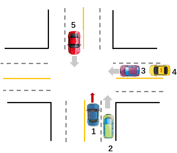
Figure 7 shows the performance of the continuous potential game in a specific scenario, where all vehicles follow the NE strategies. The speed of each vehicle is shown in the top left corner in Figures 7 and 7. The ego vehicle first slows down to yield to the purple and yellow vehicles (Figure 7) and then speeds up after these two vehicles cross the intersection (Figure 7). The performance of the best response dynamics and of the potential function optimization algorithm are very close in this scenario. (Comparative animations are available at https://youtu.be/nQkpdQRcwEE). The iterations of the best response dynamics are shown in Figures 7 and 7, at the time instance illustrated in Figure 7 and that of Figure 7, respectively, validating the convergence of the best response dynamics.
We also consider the scenarios where the surrounding vehicles do not take the NE strategies. In these scenarios, the potential function optimization algorithm outperforms the best response dynamics in terms of better safety performance. The specific scenarios are shown in the first part of the intersection-crossing animation at https://youtu.be/nQkpdQRcwEE, and the statistical comparison is shown in the next subsection.


V-C Statistical comparison of various potential game algorithms
In this subsection, we conduct two comparative studies in intersection-crossing scenarios: 1) finite potential game vs. continuous potential game, and 2) best response dynamics vs. potential function optimization algorithm. For each study, the comparisons are conducted in terms of a) computational efficiency measured by the average and maximum computational time to complete one decision-making process, b) the ego vehicle safety measured by the collision rate, average and maximum collision speeds, and c) the ego vehicle travel efficiency measured by the ego vehicle average speed during the intersection-crossing. As for the surrounding vehicles, we assign them three different strategies: a) employing the NE, b) keeping a constant speed, and c) randomly selecting an acceleration from the action space at each . The first strategy is rational and intelligent. The second strategy is non-intelligent and safety-agnostic, but may be encountered in real scenarios as human driver may be distracted from driving and therefore cannot respond timely to a collision threat. The third strategy is neither intelligent nor rational but useful for testing robustness of the algorithms. For each algorithm, we test intersection situations with randomly selected vehicles’ initial positions to provide reliable statistical results. In each situation, vehicles get involved (as shown in Figure 6), i.e., the ego vehicle solves a -player game for each decision-making.
Table I shows the comparative results between finite potential game and continuous potential game. The running time is collected from MATLAB® on a laptop with an Intel Core i7-10750H processor clocked at GHz and GB of RAM. We use the genetic algorithm function ’ga’ in Matlab [41, 42] to efficiently solve the non-convex optimization problems. For potential function optimization (Algorithm 2), start points are selected, and for best response dynamics (Algorithm 1), start points are selected for each agent’s local optimization. The number of start points is selected based on the criterion that increasing this number does not necessarily improve the ego vehicle performance (in terms of collision rate and average velocity) while decreasing this number clearly leads to worse performance. The collision rate represents the number of situations where a collision happens to the ego vehicle out of the total number of situations (i.e., ). Concerning the average speed, note that the ego vehicle desired speed is , and in general, the closer the average speed to , the better the travel efficiency of the ego vehicle. The average and maximum ego vehicle speed at collision indicates the contribution of the ego vehicle to the collision impact, which relates to the two vehicles’ relative speed. The action space of each vehicle is: for continuous game and for finite game. For both potential games, the NE is determined by the potential function optimization algorithm, i.e., Algorithm 1.
| Finite potential game | Continuous potential game | |||||
| Surrounding vehicles’ strategies | NE | Constant speed | Random acceleration | NE | Constant speed | Random acceleration |
| Collision rate | ||||||
| Average ego speed (m/s) | ||||||
| Avg/Max relative collision speed (m/s) | N/A | N/A | N/A | N/A | ||
| Avg/Max ego speed at collision (m/s) | N/A | N/A | N/A | N/A | ||
| Avg/Max computational time (s) | ||||||
Table I leads to the following observations:
- 1.
Both potential game frameworks are effective in ensuring the ego vehicle safety: No collision happens in any of the scenarios if the surrounding vehicles follow the NE strategies or maintain constant speeds. Although absolute safety is not guaranteed if the surrounding vehicles randomly accelerates at each (which is too irrational to happen in real life), the collision rate is still low (less than ).
- 2.
In both games, the ego vehicle shows better travel efficiency if the surrounding vehicles follow the NE strategies, compared to the one of constant speeds. It implies that the more intelligent the surrounding vehicles are, the better the ego vehicle travel efficiency is. Meanwhile, even if the surrounding vehicles are non-intelligent (maintaining constant speeds), the ego vehicle travel efficiency remains satisfactory ( in continuous game and in finite game), while ensuring safety.
- 3.
Computational cost is affordable in both potential game frameworks (less than on average).
- 4.
In general, the continuous potential game outperforms the finite potential game, as it leads to better travel efficiency with similar safety and computation performance.
| Best response dynamics | Potential function optimization | |||||
| Surrounding vehicles’ strategies | NE | Constant speed | Random acceleration | NE | Constant speed | Random acceleration |
| Collision rate | ||||||
| Average ego speed (m/s) | ||||||
| Avg/Max relative collision speed (m/s) | N/A | N/A | N/A | |||
| Avg/Max ego speed at collision (m/s) | N/A | N/A | N/A | |||
| Avg/Max computational time (s) | ||||||
Table II compares the results from the two solution algorithms (best response dynamics and potential function optimization) in the continuous potential game framework. The simulation settings are selected to be the same as the ones for Table I.
Table II leads to the following observations:
- 1.
Both solution algorithms are effective in ensuring the ego vehicle safety when the surrounding vehicles follow the NE strategies: No collision happens in any of the scenarios. If the surrounding vehicles are non-intelligent (i.e., maintaining constant speeds or using random accelerations), the potential function optimization algorithm performs notably better than the best response dynamics. This is because the potential function optimization finds the global optimal NE, while the best response dynamics may converge to any NE.
- 2.
With regard to the ego vehicle travel efficiency, although the best response dynamics lead to higher average speeds, we cannot conclude that it has better travel efficiency. This is because the two solution algorithms have different safety levels, and although the best response dynamics result in higher speeds, it puts the ego vehicle into more dangerous situations.
- 3.
Computational cost is affordable in both solution algorithms ( in potential function optimization and in best response dynamics, on average). Compared to the best response dynamics, the potential function optimization has better computational efficiency.
- 4.
In general, the potential function optimization algorithm outperforms the best response dynamics, as it requires less computational time and leads to better safety for the ego vehicle.
V-D Statistical comparison of various AV decision-making algorithms
In this subsection, we compare potential games with other existing decision-making approaches, including reinforcement learning and control barrier function. The simulation scenarios and settings are the same as the ones in Section V-C, and the agents’ action spaces are finite.
For potential games, we employ the potential function optimization algorithm.
For reinforcement learning, we employ a double deep Q-network (DDQN) algorithm [43, 44]. Similar to the potential game, the ego vehicle’s cost function in RL is also composed of two parts: One is to track the desired speed as in (30), and the other is to avoid collision (specifically, if a collision happens, then a large penalty is applied). During the training stage, the surrounding vehicle behaviors are governed by a simplified intelligent driver model (IDM) [45]: If vehicle senses a collision threat with vehicle (i.e., inter-vehicle distance is less than a pre-defined safe distance), then vehicle brakes if and accelerates otherwise, with constant a acceleration/deceleration. Here represents time-to-collision for vehicle with vehicle (see [44, 14] for the mathematical expression). We train the RL agent for episodes, where each episode contains 24 samples (corresponds to the duration of the intersection crossing with sampling time) or less (if collisions occur). For the execution stage, we let the surrounding vehicles follow one of two strategies, NE or constant speed, to test the robustness of the performance. In this intersection-crossing scenario, the vehicle behaviors from the NE and from the IDM are very close, as they both motivate the vehicles to cooperatively avoid collisions by accelerating (resp. decelerating) the vehicle that is closer (resp. farther) from the conflict point.
For the CBF-based approach, because the ego vehicle cannot control the surrounding vehicles’ behaviors, we use a variant of the centralized CBF – the predictor-corrector collision avoidance (PCCA) of [46]. Note that differently from [46], the ego vehicle’s action space is bounded in the driving scenario. If the generated action from the CBF exceeds the bound, then the bound value is applied in our implementation.
| Potential game | Control barrier function | Reinforcement learning | ||||
| Surrounding vehicles’ strategies | NE | Constant speed | NE | Constant speed | NE | Constant speed |
| Collision rate | ||||||
| Average ego speed (m/s) | ||||||
| Avg/Max relative collision speed (m/s) | N/A | N/A | N/A | 5.23/7.07 | N/A | |
| Avg/Max ego speed at collision (m/s) | N/A | N/A | N/A | 0.72/5.00 | N/A | |
| Ave/Max computational time (s) | ||||||
The statistical comparison of the above approaches is shown in Table III. (Performance in specific scenarios is shown in the last part at https://youtu.be/nQkpdQRcwEE.) Table III leads to the following observations:
- 1.
The reinforcement learning approach performs well when the surrounding vehicles follow the NE strategies, while its performance significantly degrades when other vehicles follow the constant speed strategy. It is because the performance of RL is highly dependent on the training dataset. Since the deep Q-network is trained by IDM-governed surrounding vehicles, if a vehicle does not follow the IDM and is safety-agnostic, it can easily lead to a collision with the ego vehicle. In real world, it is extremely hard, if not impossible, to reflect all situations and all vehicle behaviors in the training dataset, and therefore, the robustness of the RL-based algorithm can be a major concern in autonomous driving.
- 2.
The control barrier function based approach is not able to ensure safety either, when the surrounding vehicles follow the constant speed strategy. It is because to guarantee the forward invariance of a pre-defined safety set, the CBF based approach generally requires all agents’ adherence to the CBF constraints [47]. In a decentralized setting where other agents may not adhere to the CBF constraints, to ensure recursive feasibility, an unbounded action space of the ego vehicle is usually required [46], which is unrealistic in driving applications.
- 3.
In contrast to RL and CBF, the potential game approach demonstrates significantly better robustness: It successfully avoids all collisions even if the surrounding vehicles follow the constant speed strategy.
- 4.
All three approaches are computationally feasible, as the running time is always less then the sampling time in all tested scenarios.
VI Conclusion
This paper developed two potential game based frameworks to formulate the process of decision-making in autonomous driving when multiple traffic agents are involved. Theoretical guarantees for the existence of NE and convergence of NE seeking algorithms were presented. Scalability challenge was addressed. Approaches to constructing potential games for autonomous driving applications were provided. By comprehensive numerical studies, we showed that our developed potential game frameworks can generate safe and effective decisions for the ego vehicle in diverse traffic scenarios including lane-changing and intersection-crossing. Comparative studies with the RL and the CBF based approaches showed that the developed potential game approach leads to the best robustness against safety-agnostic surrounding vehicles. Future work will include verification and validation of the proposed potential game approach in various traffic situations, and development of prediction and learning modules to account for uncertain intentions and/or unknown cost functions of other vehicles.
References
- [1] BuyShares, “Global autonomous car market to grow by 36 and hit a value by 2023,” https://buyshares.co.uk/global-autonomous-car-market-to-grow-by-36-and-hit-a-37b-value-by-2023/, Tech. Rep., 2021.
- [2] M. Campbell, M. Egerstedt, J. P. How, and R. M. Murray, “Autonomous driving in urban environments: approaches, lessons and challenges,” Philosophical Transactions of the Royal Society A: Mathematical, Physical and Engineering Sciences, vol. 368, no. 1928, pp. 4649–4672, 2010.
- [3] D. González, J. Pérez, V. Milanés, and F. Nashashibi, “A review of motion planning techniques for automated vehicles,” IEEE Transactions on Intelligent Transportation Systems, vol. 17, no. 4, pp. 1135–1145, 2015.
- [4] B. R. Kiran, I. Sobh, V. Talpaert, P. Mannion, A. A. Al Sallab, S. Yogamani, and P. Pérez, “Deep reinforcement learning for autonomous driving: A survey,” IEEE Transactions on Intelligent Transportation Systems, 2021.
- [5] S. Noh, “Decision-making framework for autonomous driving at road intersections: Safeguarding against collision, overly conservative behavior, and violation vehicles,” IEEE Transactions on Industrial Electronics, vol. 66, no. 4, pp. 3275–3286, 2018.
- [6] C.-J. Hoel, K. Driggs-Campbell, K. Wolff, L. Laine, and M. J. Kochenderfer, “Combining planning and deep reinforcement learning in tactical decision making for autonomous driving,” IEEE Transactions on Intelligent Vehicles, vol. 5, no. 2, pp. 294–305, 2019.
- [7] P. Hang, C. Lv, Y. Xing, C. Huang, and Z. Hu, “Human-like decision making for autonomous driving: A noncooperative game theoretic approach,” IEEE Transactions on Intelligent Transportation Systems, 2020.
- [8] A. Rasouli and J. K. Tsotsos, “Autonomous vehicles that interact with pedestrians: A survey of theory and practice,” IEEE Transactions on Intelligent Transportation Systems, vol. 21, no. 3, pp. 900–918, 2019.
- [9] L. Hou, L. Xin, S. E. Li, B. Cheng, and W. Wang, “Interactive trajectory prediction of surrounding road users for autonomous driving using structural-lstm network,” IEEE Transactions on Intelligent Transportation Systems, vol. 21, no. 11, pp. 4615–4625, 2019.
- [10] C. Xu, W. Zhao, L. Li, Q. Chen, D. Kuang, and J. Zhou, “A nash q-learning based motion decision algorithm with considering interaction to traffic participants,” IEEE Transactions on Vehicular Technology, vol. 69, no. 11, pp. 12 621–12 634, 2020.
- [11] N. Li, D. W. Oyler, M. Zhang, Y. Yildiz, I. Kolmanovsky, and A. R. Girard, “Game theoretic modeling of driver and vehicle interactions for verification and validation of autonomous vehicle control systems,” IEEE Transactions on Control Systems Technology, vol. 26, no. 5, pp. 1782–1797, 2017.
- [12] Q. Zhang, R. Langari, H. E. Tseng, D. Filev, S. Szwabowski, and S. Coskun, “A game theoretic model predictive controller with aggressiveness estimation for mandatory lane change,” IEEE Transactions on Intelligent Vehicles, vol. 5, no. 1, pp. 75–89, 2019.
- [13] V. Lopez, F. Lewis, M. Liu, Y. Wan, S. Nageshrao, and D. Filev, “Game-theoretic lane-changing decision making and payoff learning for autonomous vehicles,” IEEE Transactions on Vehicular Technology, 2022.
- [14] M. Liu, Y. Wan, F. Lewis, S. Nageshrao, and D. Filev, “A three-level game-theoretic decision-making framework for autonomous vehicles,” IEEE Transactions on Intelligent Transportation Systems, 2022.
- [15] F. Camara, N. Bellotto, S. Cosar, F. Weber, D. Nathanael, M. Althoff, J. Wu, J. Ruenz, A. Dietrich, G. Markkula et al., “Pedestrian models for autonomous driving part ii: high-level models of human behavior,” IEEE Transactions on Intelligent Transportation Systems, 2020.
- [16] H. Kita, “A merging–giveway interaction model of cars in a merging section: a game theoretic analysis,” Transportation Research Part A: Policy and Practice, vol. 33, no. 3-4, pp. 305–312, 1999.
- [17] N. Li, Y. Yao, I. Kolmanovsky, E. Atkins, and A. R. Girard, “Game-theoretic modeling of multi-vehicle interactions at uncontrolled intersections,” IEEE Transactions on Intelligent Transportation Systems, 2020.
- [18] Q. Dai, X. Xu, W. Guo, S. Huang, and D. Filev, “Towards a systematic computational framework for modeling multi-agent decision-making at micro level for smart vehicles in a smart world,” Robotics and Autonomous Systems, vol. 144, p. 103859, 2021.
- [19] D. Monderer and L. S. Shapley, “Potential games,” Games and economic behavior, vol. 14, no. 1, pp. 124–143, 1996.
- [20] D. Cai, S. Bose, and A. Wierman, “On the role of a market maker in networked cournot competition,” Mathematics of Operations Research, vol. 44, no. 3, pp. 1122–1144, 2019.
- [21] J. Wu and D. Zusai, “A potential game approach to modelling evolution in a connected society,” Nature human behaviour, vol. 3, no. 6, pp. 604–610, 2019.
- [22] K. Yamamoto, “A comprehensive survey of potential game approaches to wireless networks,” IEICE Transactions on Communications, vol. 98, no. 9, pp. 1804–1823, 2015.
- [23] Y. Hino, “An improved algorithm for detecting potential games,” International Journal of Game Theory, vol. 40, no. 1, pp. 199–205, 2011.
- [24] Y. Shoham and K. Leyton-Brown, Multiagent systems: Algorithmic, game-theoretic, and logical foundations. Cambridge University Press, 2008.
- [25] H. Lu, “On the existence of pure-strategy nash equilibrium,” Economics Letters, vol. 94, no. 3, pp. 459–462, 2007.
- [26] S. Durand and B. Gaujal, “Complexity and optimality of the best response algorithm in random potential games,” in International Symposium on Algorithmic Game Theory, 2016, pp. 40–51.
- [27] Q. D. Lã, Y. H. Chew, and B.-H. Soong, Potential Game Theory. Springer, 2016.
- [28] M. Elbanhawi, M. Simic, and R. Jazar, “In the passenger seat: investigating ride comfort measures in autonomous cars,” IEEE Intelligent transportation systems magazine, vol. 7, no. 3, pp. 4–17, 2015.
- [29] M. Zhou, Y. Yu, and X. Qu, “Development of an efficient driving strategy for connected and automated vehicles at signalized intersections: A reinforcement learning approach,” IEEE Transactions on Intelligent Transportation Systems, vol. 21, no. 1, pp. 433–443, 2019.
- [30] L. Zhang, K. Peng, X. Zhao, and A. J. Khattak, “New fuel consumption model considering vehicular speed, acceleration, and jerk,” Journal of Intelligent Transportation Systems, pp. 1–13, 2021.
- [31] Q. Dai, D. Shen, J. Wang, S. Huang, and D. Filev, “Calibration of human driving behavior and preference using naturalistic traffic data,” arXiv preprint arXiv:2105.01820, 2021.
- [32] C. Hubmann, M. Becker, D. Althoff, D. Lenz, and C. Stiller, “Decision making for autonomous driving considering interaction and uncertain prediction of surrounding vehicles,” in IEEE Intelligent Vehicles Symposium, 2017, pp. 1671–1678.
- [33] J. F. Fisac, E. Bronstein, E. Stefansson, D. Sadigh, S. S. Sastry, and A. D. Dragan, “Hierarchical game-theoretic planning for autonomous vehicles,” in International Conference on Robotics and Automation (ICRA), 2019, pp. 9590–9596.
- [34] R. Tian, N. Li, I. Kolmanovsky, Y. Yildiz, and A. R. Girard, “Game-theoretic modeling of traffic in unsignalized intersection network for autonomous vehicle control verification and validation,” IEEE Transactions on Intelligent Transportation Systems, 2020.
- [35] J. Kong, M. Pfeiffer, G. Schildbach, and F. Borrelli, “Kinematic and dynamic vehicle models for autonomous driving control design,” in IEEE intelligent vehicles symposium (IV), 2015, pp. 1094–1099.
- [36] P. Polack, F. Altché, B. d’Andréa Novel, and A. de La Fortelle, “The kinematic bicycle model: A consistent model for planning feasible trajectories for autonomous vehicles?” in IEEE intelligent vehicles symposium (IV), 2017, pp. 812–818.
- [37] L. Yang, X. Li, W. Guan, H. M. Zhang, and L. Fan, “Effect of traffic density on drivers’ lane change and overtaking maneuvers in freeway situation—a driving simulator–based study,” Traffic injury prevention, vol. 19, no. 6, pp. 594–600, 2018.
- [38] X. Cao, W. Young, and M. Sarvi, “Exploring duration of lane change execution,” in Australasian Transport Research Forum, 2013.
- [39] J. Xiao, Z. Xiao, D. Wang, V. Havyarimana, C. Liu, C. Zou, and D. Wu, “Vehicle trajectory interpolation based on ensemble transfer regression,” IEEE Transactions on Intelligent Transportation Systems, 2021.
- [40] J. Liu, L. N. Boyle, and A. Banerjee, “An inverse reinforcement learning approach for customizing automated lane change systems,” IEEE Transactions on Vehicular Technology, 2022.
- [41] MathWorks, “Find minimum of function using genetic algorithm,” https://www.mathworks.com/help/gads/ga.html.
- [42] D. I. Arkhipov, D. Wu, T. Wu, and A. C. Regan, “A parallel genetic algorithm framework for transportation planning and logistics management,” IEEE Access, vol. 8, pp. 106 506–106 515, 2020.
- [43] H. Van Hasselt, A. Guez, and D. Silver, “Deep reinforcement learning with double q-learning,” in Proceedings of the AAAI conference on artificial intelligence, vol. 30, no. 1, 2016.
- [44] S. Nageshrao, H. E. Tseng, and D. Filev, “Autonomous highway driving using deep reinforcement learning,” in 2019 IEEE International Conference on Systems, Man and Cybernetics (SMC), 2019, pp. 2326–2331.
- [45] M. Treiber, A. Hennecke, and D. Helbing, “Congested traffic states in empirical observations and microscopic simulations,” Physical review E, vol. 62, no. 2, p. 1805, 2000.
- [46] M. Santillo and M. Jankovic, “Collision free navigation with interacting, non-communicating obstacles,” in American Control Conference (ACC), 2021, pp. 1637–1643.
- [47] A. D. Ames, X. Xu, J. W. Grizzle, and P. Tabuada, “Control barrier function based quadratic programs for safety critical systems,” IEEE Transactions on Automatic Control, vol. 62, no. 8, pp. 3861–3876, 2016.
- [48] R. Williamson and H. Trotter, Multivariable Mathematics. Pearson Education, 2004.
Appendix
VI-A Proof of Proposition 1
Necessity. We first prove that if (4) holds, then (17) holds. Let be a unit vector in . If (4) holds, then the following equation holds,
| (36) |
Sufficiency. Now we prove that if (17) holds, then (4) holds. Because is a connected set, for any given and , there must exist a continuous curve that starts at and ends at . As such, (17) leads to
| (37) |
where represents the line integral along the curve . According to the gradient theorem for line integrals [48], , and . As such, Equation (37) leads to (4).
VI-B Proof of Lemma 3
Let be a NE of the game (2), i.e., . From (17), it follows that for some function , and hence , i.e., is a also NE for the identical-interest game with all agents’ cumulative costs equal to . On the other hand, if is a NE for the identical-interest game, then similar arguments imply that it is also a NE of the game (2).
VI-C Proof of Lemma 4
For continuous potential games with compact and continuous , a minimum of as a function of always exists, according to Weierstrass theorem [48]. Hence, a NE exists according to Lemma 3. If is strictly convex, then it has a unique minimum, and as such, the game has a unique NE.
![[Uncaptioned image]](2201.06157v3/mushuang.png) |
Mushuang Liu is an Assistant Professor in the Department of Mechanical and Aerospace Engineering at the University of Missouri, Columbia, MO. She worked as a Postdoc in the Department of Aerospace Engineering at the University of Michigan, Ann Arbor, MI, 2021-2022. She received her Ph.D degree from the University of Texas at Arlington in 2020 and her B.S. degree from the University of Electronic Science and Technology of China in 2016. Her research lies in control and learning for multi-agent systems. |
![[Uncaptioned image]](2201.06157v3/ilya.jpg) |
Ilya Kolmanovsky is a professor in the department of aerospace engineering at the University of Michigan, Ann Arbor, MI, USA, with research interests in control theory for systems with state and control constraints, and in control applications to aerospace and automotive systems. He received his Ph.D. degree in aerospace engineering from the University of Michigan in 1995. Prior to joining the University of Michigan as a faculty in 2010, Kolmanovsky was with Ford Research and Advanced Engineering in Dearborn, Michigan for close to 15 years. He is a Fellow of IEEE, IFAC and NAI, and a Senior Editor of IEEE Transactions on Control Systems Technology. |
![[Uncaptioned image]](2201.06157v3/Eric.jpeg) |
H. Eric Tseng received the B.S. degree from the National Taiwan University, Taipei, Taiwan, in 1986, and the M.S. and Ph.D. degrees in mechanical engineering from the University of California at Berkeley, Berkeley, in 1991 and 1994, respectively. In 1994, he joined Ford Motor Company. At Ford, he is currently a Senior Technical Leader of Controls and Automated Systems in Research and Advanced Engineering. Many of his contributed technologies led to production vehicles implementation. His technical achievements have been recognized internally seven times with Ford’s highest technical award—the Henry Ford Technology Award, as well as externally by the American Automatic Control Council with Control Engineering Practice Award in 2013. He has over 100 U.S. patents and over 120 publications. He is an NAE Member. |
![[Uncaptioned image]](2201.06157v3/shuang10.jpg) |
Suzhou Huang is an executive technical leader in Research and Advanced Engineering at Ford Motor Company. His research interests now mostly concentrate on autonomous and connected vehicle technologies, human driving behavior modeling, and smart transportation systems using methodologies of ML/AI and game theory. Prior to his current position, he was director, Analytics RD in Global Data Insights and Analytics at Ford Motor and at Ford Credit, developing advanced analytics models in a variety of areas, such as production planning, inventory management, pricing, marketing program evaluation, auto financing, risk management, capital allocation, and regulation compliance. Suzhou Huang earned a Ph.D. in theoretical physics from MIT. Since he joined Ford in 1998 he transformed himself into an applied micro-economist/econometrician. |
![[Uncaptioned image]](2201.06157v3/dimitar2.jpg) |
Dimitar Filev is Senior Henry Ford Technical Fellow in Control and AI with Research Advanced Engineering – Ford Motor Company. His research is in computational intelligence, AI and intelligent control, and their applications to autonomous driving, vehicle systems, and automotive engineering. He holds over 100 granted US patents and has been awarded with the IEEE SMCS 2008 Norbert Wiener Award and the 2015 Computational Intelligence Pioneer’s Award. Dr. Filev is a Fellow of the IEEE and a member of the National Academy of Engineering. He was President of the IEEE Systems, Man, Cybernetics Society (2016-2017). |
![[Uncaptioned image]](2201.06157v3/anouck.png) |
Anouck Girard received the Ph.D. degree in ocean engineering from the University of California at Berkeley, Berkeley, CA, USA, in 2002. She has been with the University of Michigan, Ann Arbor, MI, USA, since 2006, where she is currently a Professor of aerospace engineering. She has coauthored the book Fundamentals of Aerospace Navigation and Guidance (Cambridge University Press, 2014). Her current research interests include vehicle dynamics and control systems. She was a recipient of the Silver Shaft Teaching Award from the University of Michigan and the Best Student Paper Award from the American Society of Mechanical Engineers. |