Unitarity and Finkelstein-Kajantie problem
in diffraction hadron production

A problem of the unitarity violation in the pomeron models is well known since 1960s [1, 2, 3]. It is more related to a 3-pomeron interaction vertex rather than to a possible large intercept ($\alpha(0)>1$) of a bare pomeron. If the pomeron trajectory is linear, so $\alpha(t)=\alpha(0)+\alpha^{\prime}t$ with $\alpha(0)=1$, and the 3P-vertex, $r_{3P}$, is constant, then total hadron cross section does not depend asymptotically on hadron energy, $\sigma_{t}(s)\propto(s/s_{0})^{\alpha_{(}0)-1}={\rm const}$ ($s_{0}\sim 1{\rm GeV}^{2}$). At the same time the contribution of diffraction production of high effective mass hadron showers, separated by the large enough rapidity gaps, to $\sigma_{t}(s)$ rise with energy vigorously demonstrating inconsistency of this simplified scheme ([4], [5], [6] and references therein).

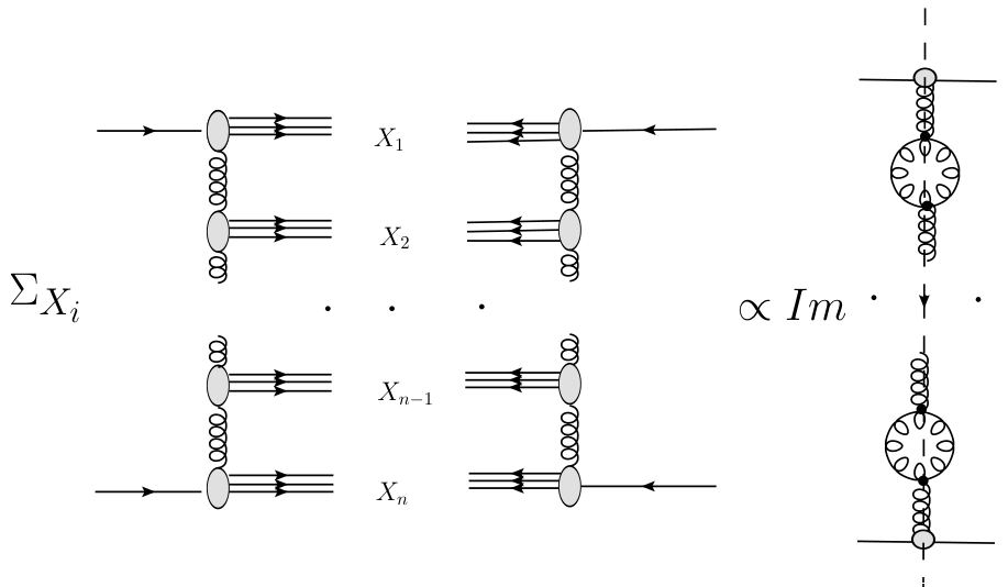
This process is pictured by the loop diagrams shown on the Fig. 2. The equivalence of left and right diagrams is a consequence of the generalized optical theorem.

Total cross section of the $n$ showers production is determined by imaginary part of the loop diagram which has in $j=\omega+1,t$-representation the following form

One can obtain from this equation that at $s\to\infty$

which comes in severe contradiction with the Froissart-Martin bound [7, 8, 9]. This is the essence of Finkelstein-Kajantie problem [2], [10], [11].

In 1970s, Cardy proposed to consider additional pomeron re-scatterings which had to screen large rapidity gaps [12]. It was believed that in a black disc limit such a screening can put the cross section back to Froissart-Martin unitarity bound [13], [14]. Unfortunately, any eikonal type screening appears to be not enough [15], [16], at least for the simplest input contribution to the amplitudes of SDD (Single Diffraction Dissociation), CDP (central Diffraction Production) or DDD (double Diffraction Dissociation). In the paper [17] the differential cross sections have been written in a general form taking into account enhanced reggeon diagrams. However, it is most likely, that the explicit final result for integrated (over rapidity and impact parameter variables) cross section cannot be obtained in analytical form. Another way to fix the problem, namely assumption that 3P-vertex depend on $t$, $r_{3P}(t)\propto t$ at $t\to 0$ [6, 18] does not supported by the data at high energies.

The pomeron with $\alpha(t)=1+\varepsilon+\alpha^{\prime}t$ as input in the eikonal ([19] and references to earlier papers therein, [20]), quasieikonal [21], $U$-matrix [22] unitarization and their generalization [23] lead to the elastic scattering amplitude which does not violate the Froissart-Martin limit for total cross section. Namely, unitarization lead to $\sigma_{t}\approx 8\pi\varepsilon\alpha^{\prime}\ln^{2}(s/s_{0})$. Such an amplitude (in a simplified form at $s\to\infty$) can be represented in impact parameter representation $H(s,b)=g\Theta(R(s)-b)$ where $R(s)\propto\ln(s/s_{0})$ and $g\leq 1$. In the $\omega$-representation this amplitude is not a pole, it looks like a pair of two complex branch points colliding at $t=0$.

Such a pomeron was called froissaron [24, 25] because it saturates the Froissart-Martin bound (in a functional form), i.e. provides the maximality of strong interactions.

By introducing the proper 3-froissaron vertex (Fig. 3), which can/must depend on spatial and angular momenta of froissarons ln it, one can hope to extend an unitarization to the shower production.

Anyway, there are two possibilities: either we start from the single pomeron pole with the intercept $\alpha(o)=1+\varepsilon>1$ (and then apply to it some a not well defined unitarization procedure) or we consider from the very beginning a more complicated pomeron singularity (for instance, in the form (3)). The question may be asked: does froissaron satisfy the Dyson-Schwinger equations (DSE), provided that the 3-froissaron vertex is chosen appropriately

The DS equation for propagator is given in the Fig. 4.

Analytically DSE for propagator has the form:

where

$\omega\equiv j-1$, $j$ is the pomeron angle momentum, $\vec{q}$ is the transverse component of the pomeron momentum, $\vec{q}\,^{2}\approx-t$.

The equation for 3-pomeron vertex $\Gamma(\omega,\omega_{1},\omega_{2};\vec{q},\vec{q}_{1},\vec{q}_{2})$ is given by the Fig. 5.

In the leading order the analytical form of DSE for 3P-vertex (if only 3P-vertices are considered) is:

where the notations $\{\omega\}=\omega,\omega^{\prime},\omega-\omega^{\prime}$, $\{q\}=\vec{q}\,^{2},\vec{q}\,^{\prime 2},(\vec{q}-\vec{q}\,^{\prime})^{2}$ are used.

General properties of DSE in the framework of Reggeon Field Theory (with the single pomeron input pole) were discussed in details by V.N. Gribov [4]. Two regimes, the weak coupling and the strong coupling ones, were analyzed. The weak coupling regime was noted as preferable, however it is not supported by available experimental data.

The first attempt to discuss the froissaron (3) as input in DSE was made by J.S. Ball [26]. He considered the model in which the output propagator and 3f-vertex are proportional to input ones

and have obtained two algebraic equations for couplings $g$ and $\gamma$.

However, one can see that in this simple scheme the integrated DSE cross section, $\sigma_{SDE}(s)=0$. We think that the problem can be fixed only if the input 3f-vertex is changed for a more complicated form.

Developing this idea is one of the goals of our work. In Section 2 we define the main ingredients in our scheme and estimate corrections to the input propagator and 3f-vertex in the DS equations. Differential and integrated cross sections of diffraction production processes are estimated at asymptotic energy in the Section 3.

We would like to emphasize here that our approach is based on two main assumptions. The first: input reggeon in DSE is a froissaron (Eq.(3)), which for $t=0$ is located in the $\omega$-plane at the point $\omega=0$ not violating the Froissart-Martin bound. The second: we assume that the 3f-vertex depends on the angular and spatial momenta of the froissarons in it, therefore the factorization of propagators and vertices takes place only in the ($\omega,t$)-representation, but does not hold in the ($s,t$) one, which is valid for input pomeron in the form of a simple pole.

In the Section 3 cross sections of diffraction processes are calculated at $s\to\infty$. The limits for free parameters at which the diffraction cross sections do not exceed Froissart-Martin bound are obtained. The results are summarized in the Conclusion.

In accordance with a general form of the elastic scattering partial amplitude at low $\omega$ and $q_{i}^{2}$ we consider the universal propagator for froissaron

where function $E(\omega,q)$ is a finite function at any $\omega,\vec{q}$, providing the main contributions in the integrals over $\omega,\vec{q}$ in the region where $\omega^{2}\approx aq^{2}\approx 0$. We remind that our main interest is concentrated in the limit of high energies and low transferred momenta, which correspond to above mentioned $\omega\to 0$.

Now we suppose that in accordance with the structure of the Froissaron singularity in $G_{0}(\omega,q)$ at $\omega^{2}+\omega_{0}^{2}=0$ the function $E(\omega,q)$ depends on $\omega$ through the variable $\kappa=(\omega^{2}+\omega_{0}^{2})^{1/2}$ and it can be expanded in powers of $\kappa$:

where $k$ corresponds (at $q=0$) to the contribution of the triple pole ($k=0)$, double pole ($k=1$) and single pole ($k=2$). Thus the frroissaron propagator can be written in the form with main and sub-asymptotic (SA corrections) terms

Let us notice that the first terms in the Eq. (10) has a pair of branch points colliding at $\omega_{0}=0\,(q=0)$ and generating a triple pole. The numerators $E_{k}(\omega,q,k=0,1,2)$ can be chosen for simplicity in exponential form either $e^{-B_{k}q}$ or $e^{-B_{k}q^{2}}$, although it can be more sophisticated. The amplitudes with such terms can be calculated in $(s,b)$-representation, or at least can be estimated at $b\ll\xi=\ln(s/s_{0})$ and $b\gg\xi=\ln(s/s_{0})$. The details for $k=0$ are given in the A.

We impose certain requirements to the vertex function, from which the intervals for the vertex parameters can be set.

1. 1.

   Vertex could not have singularities in $\omega_{i},q_{i}\sim 0$ which lead to its infinity and could not cancel a singularity of the propagator (while it can make it a more soft). It means that vertex can (must) have zeros at some of these variables.

2. 2.

   Diffractive differential and their integrated cross-sections could not violate the unitarity restriction;

3. 3.

   In accordance with the experimental data differential cross section the single diffraction dissociation does not vanish at $t=0$;

4. 4.

   Most likely, the experiments show that diffractive integrated cross sections rise with energy slowly then total and elastic integrated cross sections.

5. 5.

   Corrections to propagator and vertex in the DS-equations would be small at small $\omega_{i}$ and $q_{i}^{2}$;

We consider here the 3f-vertex function in a factorized form. Each of the three factors at the vertex (Fig. 6) depends on the type of reggeon corresponding to it in accordance with Eq. (10) and has the same functional form. Generally, the factor corresponding to the input froissaron (with $\omega_{0},\vec{q_{0}}$) can differ of other, output ones. For instance, it can have free parameters which are different from those at other factors shown in the next equations. We don’t consider here such a possibility in order to avoid a non-principal complexity.

where

and

with $\mu_{1}(k)$ coming from the 3f-vertex while the second term $k$ takes into account the kind of reggeon from the expansion (10) of the f-propagator.

To satisfy the point 1 from the list of requirements to 3f-vertex we must impose

It will be shown in the Section 3.1 that $\mu_{1}(k=0)\equiv\mu_{0}\neq 0$. Otherwise this term leads to the integrated diffraction cross section rising with energy $\propto\ln^{5}(s/s_{0})$ (F-K problem).

In the next Sections we consider three specified choices of the function $\mu_{1}(k)$

Variant a) chooses the universal form of 3f-vertex independent on the corrections to propagators. Variants b) and c) describe an increasing and decreasing with $k$ power of $\kappa$ in the vertex.

Now let’s consider a smallness of the corrections to propagator $G_{0}(\omega,t)$ and vertex $\Gamma_{0}(\{\omega\},\{\vec{q}\})$.

References

• [1] I.A. Verdiev, O.V. Kanchelli, S.G. Matinyan, A.M. Popova, K.A. Ter-Martirosyan, Sov. Phys. JETP 19 (1964), 1148.
• [2] J. Finkelstein, K. Kajantie, Multiple Pomeranchuk exchange violates unitarity, Phys. Lett. 26 B (1968), 305; Total cross-section for n-particle production in a multi-Regge model, Nuovo Cimento 56 A, (1968) 659.
• [3] V.N. Gribov, A. A. Migdal, Properties of the pomeranchuk pole and the branch cuts related to it at low momentum transfer, Sov. J. Nucl. Phys. 8 (1969) 583.
• [4] V.N. Gribov, The Theory of Complex Angular Momentum, Cambridge University Press (2003).
• [5] A.B. Kaidalov and K.A. Ter-Martirosyan, Nucl. Phys. B 75 (1974) 471.
• [6] A.B. Kaidalov, Diffractive production mechanisms, Phys. Rep. 50 (1979) 157.
• [7] M. Froissart, Asymptotic behavior and subtractions in the Mandelstam representation, Phys. Rev.123 (1961) 1053.
• [8] A. Martin, Extension of the Axiomatic Analyticity Domain of Scattering Amplitudes by Unitarity - I; Nuovo Cimento 42 A (1966) 930.
• [9] L. Łukaszuk, L., Martin, A. Absolute upper bounds for π​π\pi\pi scattering, Nuovo Cimento 52 A (1967) 122.
• [10] H.D.I. Abarbanel, J.P. Bronzan, R.L. Sugar, A.R. White, Phys. Rept. 21 (1975), 119.
• [11] R.C. Brower and J. H. Weis, Pomeron decoupling theorems, Rev. Mod. Phys. 47, 605.
• [12] J.L. Cardy, General features of the reggeon calculus with α>1\alpha>1, Nucl. Phys. B 75 (1974), 413.
• [13] E.Gotsman, E.M.Levin and U.Maor, Diffractive dissociation and eikonalization in high energy pp and ¯pp collisions, Phys.Rev. D 49 (1994) 4321.
• [14] V.V. Khoze, A. D. Martin, and M. G. Ryskin, High energy elastic and diffractive cross sections, Eur. Phys. J. C 74 (2014) 2756.
• [15] E.S. Martynov, B.V. Struminsky, Unitarized model of hadronic diffractive dissociation, Phys. Rev. D 53 (1996) 1018.
• [16] E. Martynov, G. Tersimonov, Multigap diffraction cross sections: Problems in eikonal methods for the Pomeron unitarization, Phys. Rev. D 101 (2020) 114003.
• [17] V.A. Khoze, A.D. Martin, M.G. Ryskin, Dynamics of diffractive dissociation, Eur.Phys.J. C 81 (2021) 2, 175.
• [18] R.C. Brower, E. De Tar, J.H. Weis, Regge theory for multiparticle amplitudes, Phys. Rep. 14 (1974) 257.
• [19] Collins, P.D.B. An introduction to Regge theory & high energy physics. Cambridge University press. 1977.
• [20] H. Cheng, T.T. Wu, Limit of Cross Sections at Infinite Energy, Phys. Rev. Lett. 24 (1970) 1456.
• [21] K.A. Ter-Martirosyan, The "quasi-eikonal" approximation, Pisma Zh. Eksp. Teor. Fiz. 15 (1972) 734.
• [22] S. M. Troshin, N. E. Tyurin, Unitarity at the LHC energies, Phys. Part. Nucl. 35 (2004) 555.
• [23] J.-R. Cudell, E. Predazzi, O. V. Selyugin, New analytic unitarization schemes, Phys. Rev. D 79 (2009), 034033.
• [24] M.S. Dubovikov, B. Z. Kopellovich, L.I. Lapidus, K.A. Ter-Martirosyan, Nuclear Physics B 123 (1977) 147.
• [25] K.A. Ter-Martirosyan, M.S. Dubovikov, Theory of froissaron exchange, Nuclear Physics, B 124 (1977) 163-188. doi: 10.1016/0550-3213(77)90283-8
• [26] James S. Ball, An exact solution to reggeon calculus, Nucl. Phys., B 102 (1976) 347.
• [27] E. Martynov, B. Nicolescu, Did TOTEM experiment discover the Odderon?, Phys. Lett. B 778 (2018) 414 .
• [28] E. Martynov, B. Nicolescu, Evidence for maximality of strong interactions from LHC forward data, Phys. Lett. B 786 (2018) 207 .
• [29] E. Martynov, B. Nicolescu, Odderon effects in the differential cross-sections at Tevatron and LHC energies, Eur. Phys. J. C 79 (2019) 461.
• [30] I.S. Gradshteyn and I.M. Ryzhik, Table of Integrals, Series, and Products. 2007, Elsevier Inc.
Appendix A Modified propagator for reggeon
Let us consider the possibility to have a smooth behavior of Im​H(k)​(s,b)\text{Im}H^{(k)}(s,b) in bb and to guarantee a divergence of integrals over momenta qi→\vec{q_{i}}. For that we write a reggeon propagators in the following form
G(k)(ω,q)=gk​e−B​q2(ω2+a2​q2)3/2−k/2,k=0,1,2G^{(k)}(\omega,q)=\dfrac{g_{k}e^{-Bq^{2}}}{(\omega^{2}+a^{2}q^{2})^{3/2-k/2}},\quad k=0,1,2 (A.1)
Im​H(k)​(s,b)=v2​gk4​s​Im​(i​∫0∞d​q​q​J0​(b​q)​e−B​q2​∫d​ω2​π​i​e(1+ω)​ξ′(ω2+a2​q2)3/2−k/2)=CIm(iξ′1−k/2∫0∞dxxk/2J0(bx/a)e−Bx2/a2J1−k/2(ξ′x)),C=v2gkπ2−k/28​s0​a2​Γ​(3/2−k/2),ξ′=ξ−iπ/2.\begin{array}[]{{rl}}\text{Im}H^{(k)}(s,b)&=\dfrac{v^{2}g_{k}}{4s}\text{Im}\left(i\int\limits_{0}^{\infty}dqqJ_{0}(bq)e^{-Bq^{2}}\int\dfrac{d\omega}{2\pi i}\dfrac{e^{(1+\omega)\xi^{\prime}}}{(\omega^{2}+a^{2}q^{2})^{3/2-k/2}}\right)\\ &=C\text{Im}\left(i\xi^{\prime 1-k/2}\int\limits_{0}^{\infty}dxx^{k/2}J_{0}(bx/a)e^{-Bx^{2}/a^{2}}J_{1-k/2}(\xi^{\prime}x)\right),\\ C&=\dfrac{v^{2}g_{k}\sqrt{\pi}2^{-k/2}}{8s_{0}a^{2}\Gamma(3/2-k/2)},\quad\xi^{\prime}=\xi-i\pi/2.\end{array} (A.2)
Then considering ξ→∞\xi\to\infty we neglect the imaginary part in ξ′\xi^{\prime} and make use the integral ([30])
∫0∞dxxλ−1e−α​x2Jμ(βx)Jν(γx)=βμ​γν2ν+μ+1​Γ​(ν+1)α−(λ+ν+μ)/2×∑m=0∞Γ⁡(m+(λ+μ+ν)/2)m!​Γ​(m+μ+1)​(−β24​α2)m×F⁡(−m,−m−μ,ν+1,γ2β2).\begin{array}[]{ll}&\int\limits_{0}^{\infty}dxx^{\lambda-1}e^{-\alpha x^{2}}J_{\mu}(\beta x)J_{\nu}(\gamma x)=\dfrac{\beta^{\mu}\gamma^{\nu}}{2^{\nu+\mu+1}\Gamma(\nu+1)}\alpha^{-(\lambda+\nu+\mu)/2}\\ &\times\sum\limits_{m=0}^{\infty}\dfrac{\Gamma(m+(\lambda+\mu+\nu)/2)}{m!\Gamma(m+\mu+1)}\left(-\dfrac{\beta^{2}}{4\alpha^{2}}\right)^{m}\\ &\times F\left(-m,-m-\mu;\nu+1;\dfrac{\gamma^{2}}{\beta^{2}}\right).\end{array}
For a​ξ≪ba\xi\ll b we choose (μ=0,ν=1−k,λ=k+1,γ=ξ,β=b/a\mu=0,\nu=1-k,\lambda=k+1,\gamma=\xi,\beta=b/a)
Im​H(k)​(s,b)=C1​∑m=0∞(−1)mm!​F​(−m,−m,2−k,ξ2(b/a)2)​(b24​(B/a)2)m≈C1​∑m=0∞(−1)mm!​(b24​(B/a)2)m=C1​exp⁡(−b24​(B/a)2),C1=C​a2​ξ1−k22−k​Γ​(2−k)​B.\begin{array}[]{rl}\text{Im}H^{(k)}(s,b)&=C_{1}\sum\limits_{m=0}^{\infty}\dfrac{(-1)^{m}}{m!}F\left(-m,-m;2-k;\dfrac{\xi^{2}}{(b/a)^{2}}\right)\left(\dfrac{b^{2}}{4(B/a)^{2}}\right)^{m}\\ &\approx C_{1}\sum\limits_{m=0}^{\infty}\dfrac{(-1)^{m}}{m!}\left(\dfrac{b^{2}}{4(B/a)^{2}}\right)^{m}=C_{1}\exp\left(-\dfrac{b^{2}}{4(B/a)^{2}}\right),\\ C_{1}&=C\dfrac{a^{2}\xi^{1-k}}{2^{2-k}\Gamma(2-k)B}.\end{array}
The estimation is valid for any considered kk.
For a​ξ≫ba\xi\gg b we choose (ν=0,μ=1−k,λ=k+,α=B/(a)2,γ=b/a,β=ξ\nu=0,\mu=1-k,\lambda=k+,\alpha=B/(a)^{2},\gamma=b/a,\beta=\xi). Then
Im​H(k)​(s,b)=C1​∑m=0∞(−)mΓ⁡(m+2−k)​(ξ24​B2/a4)m×F⁡(−m,−m+k−1,1,(b/a)2ξ2)≈C1​∑m=0∞(−1)mΓ⁡(m+2−k)​(ξ24​B2/a4)m.\begin{array}[]{rl}\text{Im}H^{(k)}(s,b)&=C_{1}\sum\limits_{m=0}^{\infty}\dfrac{(-)^{m}}{\Gamma(m+2-k)}\left(\dfrac{\xi^{2}}{4B^{2}/a^{4}}\right)^{m}\\ &\times F\left(-m,-m+k-1;1;\dfrac{(b/a)^{2}}{\xi^{2}}\right)\\ &\approx C_{1}\sum\limits_{m=0}^{\infty}\dfrac{(-1)^{m}}{\Gamma(m+2-k)}\left(\dfrac{\xi^{2}}{4B^{2}/a^{4}}\right)^{m}.\end{array}
The series in the last equation can be summed separately for k=0,1,2k=0,1,2
Im ​H(k)​(s,b)={v2​gk​B4​s0​a4(1−e−a4ξ2/4B2),k=0,v2​gk​B2​s0​a4e−a4ξ2/4B2erfi(ξa2/2B),k=1,\text{Im }H^{(k)}(s,b)=\left\{\begin{array}[]{lll}&\dfrac{v^{2}g_{k}B}{4s_{0}a^{4}}\left(1-e^{-a^{4}\xi^{2}/4B^{2}}\right),&k=0,\\ &\dfrac{v^{2}g_{k}B}{2s_{0}a^{4}}e^{-a^{4}\xi^{2}/4B^{2}}\text{erfi}(\xi a^{2}/2B),&k=1,\\ \end{array}\right.
Such a suppression factor doesn’t allow to calculate analytically the integrals for H⁡(s,b)H(s,b). However, integral for H(0)H^{(0)} was calculated numerically. The results are given at Fig. 13 for e−B​q2e^{-Bq^{2}}. At high energies, the tripole contribution G(0)​(ω,q)G^{(0)}(\omega,q) is dominating; dipole and simple pole give just the small corrections.
Refer to caption
Figure 13: Amplitude Im​H(0)​(s,b)\text{Im}H^{(0)}(s,b) calculated for propagator (A.1) at C=1,a=0.3​ Gev−1,B=2​ Gev−2C=1,a=0.3\text{\,\,Gev}^{-1},B=2\text{\,\,Gev}^{-2}.
Similar estimations and results one can obtain for the propagator
G(k)(ω,q)=gk​e−B​q(ω2+a2​q2)3/2−k,k=0,1,2.G^{(k)}(\omega,q)=\dfrac{g_{k}e^{-Bq}}{(\omega^{2}+a^{2}q^{2})^{3/2-k}},\quad k=0,1,2. (A.3)
Appendix B Restrictions on the parameters μ0,λ\mu_{0},\lambda
From the properties of 3f-vertex considered in the Section 2 we have
1. 1.
Γ0(k0,k1,k2)∝κiμ​(k),\displaystyle\Gamma_{0}^{(k_{0},k_{1},k_{2})}\propto\kappa_{i}^{\mu}(k), (B.1)
OPENb)\displaystyle b) μ⁡(k)=μ0​(1+λ​k),\displaystyle\mu(k)=\mu_{0}(1+\lambda k),
OPENc)\displaystyle c) μ⁡(k)=μ0​11+λ​k,\displaystyle\mu(k)=\mu_{0}\dfrac{1}{1+\lambda k},
2. 2.
μ⁡(k)>0k=0,1,2because vertex has no infinity at any k\mu(k)>0\quad k=0,1,2\quad\text{because vertex has no infinity at any k} (B.2)
3. 3.
μ⁡(k)<3−kk=0,1,2because vertex does not cancel zero in\displaystyle\mu(k)<3-k\quad k=0,1,2\quad\text{because vertex does not cancel zero in} (B.3)
(G0(k))−1∝κ(3−k).\displaystyle(G_{0}^{(k)})^{-1}\propto\kappa^{(3-k)}.
Besides, we know from the smallness of corrections to main contribution (all k=0k=0) that μ0>1\mu_{0}>1. Thus
0<μ⁡(k)<3−k,1<μ0<3.0<\mu(k)<3-k,\quad 1<\mu_{0}<3. (B.4)
It follows from the above inequalities that at any k≠0k\neq 0
1+λk>0⇒λ>−1/k,⇒λ>−1/2.1+\lambda k>0\Rightarrow\lambda>-1/k,\Rightarrow\lambda>-1/2. (B.5)
Variant b)
0<μ0​(1+λ​k)<3−k,1<μ0<3,⇒1<μ0<3−k1+λ​k.0<\mu_{0}(1+\lambda k)<3-k,\quad 1<\mu_{0}<3,\Rightarrow 1<\mu_{0}<\dfrac{3-k}{1+\lambda k}. (B.6)
It follows from the last inequality that
3−k1+λ​k>1,⇒λ<2−kk=2/k−1\dfrac{3-k}{1+\lambda k}>1,\Rightarrow\lambda<\dfrac{2-k}{k}=2/k-1 (B.7)
The inequality for λ\lambda should be valid for any kk, hence λ<0\lambda<0. Thus for the variant b) we have
−1/2<λ<0.-1/2<\lambda<0. (B.8)
However, it follows from the convergence of the integrals over ω\omega for cut reggeons at q=0q=0 in evaluation of CDP cross sections, that
3−2μ0>0,⇒μ0<3/2,\displaystyle 3-2\mu_{0}>0,\Rightarrow\mu_{0}<3/2, (B.9)
3−2μ(k)−k>0,k=1,⇒2−2μ(1)>0,⇒μ(1)<1,\displaystyle 3-2\mu(k)-k>0,k=1,\Rightarrow 2-2\mu(1)>0,\Rightarrow\mu(1)<1,
3−2μ(k)−k>0,k=2,⇒1−2μ(2)>0,⇒μ(2)<1/2.\displaystyle 3-2\mu(k)-k>0,k=2,\Rightarrow 1-2\mu(2)>0,\Rightarrow\mu(2)<1/2.
Hence, at λ≠0\lambda\neq 0
μ⁡(1)\displaystyle\mu(1) =μ0​(1+1​λ)<1⇒1<μ0<1(1+λ)⇒λ<0,\displaystyle=\mu_{0}(1+1\lambda)<1\Rightarrow 1<\mu_{0}<\dfrac{1}{(1+\lambda)}\Rightarrow\lambda<0, (B.10)
μ⁡(2)\displaystyle\mu(2) =μ0(1+2λ)<1/2⇒1<μ0<12​(1+2​λ)⇒λ<−1/4.\displaystyle=\mu_{0}(1+2\lambda)<1/2\Rightarrow 1<\mu_{0}<\dfrac{1}{2(1+2\lambda)}\Rightarrow\lambda<-1/4.
So, the final result for λ\lambda in the case b) is
−1/2<λ<−1/4.-1/2<\lambda<-1/4. (B.11)
Similarly for the variant c)
λ>0.\lambda>0. (B.12)
Appendix C Estimation of SDD cross section
To estimate IS​D​D​(ξ)I_{SDD}(\xi), we rewrite it as
IS​D​D​(ξ)=∫δ1−δd​x​xα1−1​(1−x)α2−1I_{SDD}(\xi)=\int\limits_{\delta}^{1-\delta}dxx^{\alpha_{1}-1}(1-x)^{\alpha_{2}-1}
where δ=ξ0/ξ<<1,≠0\delta=\xi_{0}/\xi<<1,\neq 0 and α1=3−μ⁡(k0)−k0>0,α2=3−μ⁡(k1)−μ⁡(k2)−k1−k2\alpha_{1}=3-\mu(k_{0})-k_{0}>0,\quad\alpha_{2}=3-\mu(k_{1})-\mu(k_{2})-k_{1}-k_{2} (sign of α2\alpha_{2} depends on the values of kik_{i}).
Let us split the integration domain: (δ,ϵ),(ϵ,1−ϵ),(1−ϵ,1−δ)(\delta,\epsilon),(\epsilon,1-\epsilon),(1-\epsilon,1-\delta) where ϵ\epsilon is constant, δ≪ϵ≪1\delta\ll\epsilon\ll 1. Then
IS​D​D​(ξ)\displaystyle I_{SDD}(\xi) ≈=∫δϵdx(xα1−1+xα2−1)+C=c1α1(ϵα1−δα1)−c2α2(ϵα2−δα2)+C\displaystyle\approx=\int\limits_{\delta}^{\epsilon}dx(x^{\alpha_{1}-1}+x^{\alpha_{2}-1})+\text{C}=\dfrac{c_{1}}{\alpha_{1}}(\epsilon^{\alpha_{1}}-\delta^{\alpha_{1}})-\dfrac{c_{2}}{\alpha_{2}}(\epsilon^{\alpha_{2}}-\delta^{\alpha_{2}})+C
≈{constantifα2>0,c2α2​(ξ/ξ0)−α2,ifα2<0\displaystyle\approx\left\{\begin{aligned} &&\text{constant}\quad\text{if}\quad\alpha_{2}>0,\\ &&\dfrac{c_{2}}{\alpha_{2}}(\xi/\xi_{0})^{-\alpha_{2}},\quad\text{if}\quad\alpha_{2}<0\end{aligned}\right.
where C is a constant.
We have obtained in the Section 2 that a smallness of corrections in the DS equations requires μ0>1\mu_{0}>1. Therefore, the following inequalities should be satisfied for the cases b) and c) from the Eq. (15)
μ1(k)=μ(k)+k,ifλ≠0then  1+λk>0andλ>−1/2,\displaystyle\mu_{1}(k)=\mu(k)+k,\quad\text{if}\,\,\lambda\neq 0\quad\text{then}\,\,1+\lambda k>0\,\,\text{and}\,\,\lambda>-1/2, (C.1)
OPENa)\displaystyle\rm{a)} 1<μ0<3,\displaystyle 1<\mu_{0}<3,
OPENb)\displaystyle\rm{b)} 1<μ0<3−k1+λ​k,\displaystyle 1<\mu_{0}<\dfrac{3-k}{1+\lambda k},
OPENc)\displaystyle\rm{c)} 1<μ0<(3−k)​(1+λ​k)\displaystyle 1<\mu_{0}<(3-k)(1+\lambda k)
where k=0,1,2k=0,1,2. Whence, taking into account inequalities μ⁡(k)>0,μ0>1\mu(k)>0,\mu_{0}>1 and consequently 1+λ​k>01+\lambda k>0, it follows that
b)1<μ0<11+2​λ,−1/2<λ<0,\displaystyle{\rm\displaystyle b)}\quad 1<\mu_{0}<\frac{1}{1+2\lambda},\quad-1/2<\lambda<0, (C.2)
OPENc)1<μ0<1+2​λ,λ>0.\displaystyle{\rm\displaystyle c)}\quad 1<\mu_{0}<1+2\lambda,\quad\phantom{|-1/2<}\lambda>0.
Thus, with obtained restrictions on λ\lambda we have
σS​D​D(s)∝ξ2−3​(μ0−1)×{OPENb)ξλ​μ0​(k0+k1+k2),−1/2<λ<0,OPENc)ξ−λμ0∑i=02ki1+λ​ki,λ>0.\sigma_{SDD}(s)\propto\xi^{2-3(\mu_{0}-1)}\times\left\{\begin{aligned} b)&\quad\xi^{\lambda\mu_{0}(k_{0}+k_{1}+k_{2})},\,\,&-1/2<\lambda<0,\\ c)&\quad\xi^{-\lambda\mu_{0}\sum\limits_{i=0}^{2}\dfrac{k_{i}}{1+\lambda k_{i}}},&\lambda>0.\end{aligned}\right. (C.3)